Faster Kernels for Graphs with Continuous Attributes via Hashing

Abstract

While state-of-the-art kernels for graphs with discrete labels scale well to graphs with thousands of nodes, the few existing kernels for graphs with continuous attributes, unfortunately, do not scale well. To overcome this limitation, we present hash graph kernels, a general framework to derive kernels for graphs with continuous attributes from discrete ones. The idea is to iteratively turn continuous attributes into discrete labels using randomized hash functions. We illustrate hash graph kernels for the Weisfeiler-Lehman subtree kernel and for the shortest-path kernel. The resulting novel graph kernels are shown to be, both, able to handle graphs with continuous attributes and scalable to large graphs and data sets. This is supported by our theoretical analysis and demonstrated by an extensive experimental evaluation.

I Introduction

In several domains like chemo- and bioinformatics as well as social network and image analysis structured objects appear naturally. Graph kernels are a key concept for the application of kernel methods to structured data and various approaches have been developed in recent years, see Vis+2010Neu+2015, and references therein. The considered graphs can be distinguished in (i) graphs with discrete labels, e.g., molecular graphs, where nodes are annotated by the symbols of the atoms they represent, and (ii) attributed graphs with (multi-dimensional) real-valued labels in addition to discrete labels. Attributed graphs often appear in domains like bioinformatics [3] or image classification [4], where attributes may represent physical properties of protein secondary structure elements or RGB values of colors, respectively. Taking the continuous information into account has been proven empirically to be beneficial in several applications, e.g., see [2, 3, 5, 4, 6, 7].

Kernels are equivalent to the inner product in an associated feature space, where a feature map assigns the objects of the input space to a feature vector. The various graph kernels proposed in recent years can be divided into approaches that either compute feature maps (i) explicitly, or (ii) implicitly [8]. Explicit computation schemes have been shown to be scalable and allow the use of fast linear support vector classifiers, e.g., [9], while implicit computation schemes are often slow. Alternatively, we may divide graph kernels according to their ability to handle annotations of nodes and edges. The proposed graph kernels are either (i) restricted to discrete labels, or (ii) compare annotations like continuous values by user-specified kernels. Typically kernels of the first category implicitly compare annotations of nodes and edges by the Dirac kernel, which requires values to match exactly and is not adequate for continuous values. The two classifications of graph kernels mentioned above largely coincide: Graph kernels supporting complex annotations use implicit computation schemes and do not scale well. Whereas graphs with discrete labels can be compared efficiently by graph kernels based on explicit feature maps. This is what we make use of to develop a unifying treatment. But first, let us touch upon related work.

I-A Previous work

In recent years, various graph kernels have been proposed. In [10] and [11] graph kernels were proposed based on random walks, which count the number of walks two graphs have in common. Since then, random walk kernels have been studied intensively, e.g., [12, 8, 13, 1]. Kernels based on tree patterns were initially proposed in [14]. These two approaches were originally applied to graphs with discrete labels, but the method of implicit computation supports comparing attributes by user-specified kernel functions. Kernels based on shortest paths [15] are computed by performing $1$-step walks on the transformed input graphs, where edges are annotated with shortest-path lengths. A drawback of the approaches mentioned above is their high computational cost.

A different line in the development of graph kernels focused particularly on scalable graph kernels. These kernels are typically computed efficiently by explicit feature maps, but are severely limited to graphs with discrete labels. Prominent examples are kernels based on subgraphs up to a fixed size, e.g., [16], or specific subgraphs like cycles and trees [17]. Other approaches of this category encode the neighborhood of every node by different techniques [18, 2, 19].

Recently, several kernels specifically designed for graphs with continuous attributes were proposed [5, 6, 7], and their experimental evaluation confirms the importance of handling continuous attributes adequately.

Several articles on scalable kernels for graphs with discrete labels propose the adaption of their approach to graphs with continuous attributes as future work, e.g., see [16, 19]. Yet, only little work in this direction has been reported, which is most likely due to the fact that this in general is a non-trivial task. An immediate approach is to discretize continuous values by binning. A key problem of this method is that two values, which only differ marginally may still fall in different bins and are then considered non-matching. Still, promising experimental results of such approaches have been reported for certain data sets, e.g., [2].

I-B Our Contribution

We introduce hash graph kernels for graphs with continuous attributes. This family of kernels is obtained by a generic method, which iteratively hashes continuous attributes to discrete labels in order to apply a base kernel for graphs with discrete labels. This allows to construct a single combined feature vector for a graph from the individual feature vectors of each iteration. The essence of this approach is:

The hash graph kernel framework lifts every graph kernel that supports discrete labels to a kernel which can handle continuous attributes.

We exemplify this for two established graph kernels:

• We obtain a variation of the Weisfeiler-Lehman subtree kernel, which implicitly employs a non-trivial kernel on the node and edge annotations and is suitable for continuous values.

• Moreover, we derive a variant of the shortest-path kernel which also supports continuous attributes while being efficiently computable by explicit feature maps.

For both kernels we provide a detailed theoretical analysis. Moreover, the effectiveness of these kernels is demonstrated in an extensive experimental study on real-world and synthetic data sets. The results show that hash graph kernels are orders of magnitude faster than state-of-the-art kernels for attributed graphs without drop in classification accuracy.

II Notation

An (undirected) graph $G$ is a pair $(V,E)$ with a finite set of nodes $V$ and a set of edges $E\subseteq\{\{u,v\}\subseteq V\mid u\neq v\}$. We denote the set of nodes and the set of edges of $G$ by $V(G)$ and $E(G)$, respectively. For ease of notation we denote the edge $\{u,v\}$ in $E(G)$ by $(u,v)$ or $(v,u)$. Moreover, $N(v)$ denotes the neighborhood of $v$ in $V(G)$, i.e., $N(v)=\{v^{\prime}\in V(G)\mid(v,v^{\prime})\in E(G)\}$. An attributed graph is a graph $G$ endowed with an attribute function $a\colon V(G)\to\mathbb{R}^{d}$ for $d\geq 1$. We say that $a(v)$ is an attribute of $v$ for $v$ in $V(G)$. A labeled graph is an attributed graph with an attribute function $l$, where the codomain of $l$ is restricted to a (finite) alphabet, e.g., a finite subset of the natural numbers. Analogously, we say that $l(v)$ is a label of $v$ in $V(G)$.

Let $\chi$ be a non-empty set and let $k\colon\chi\times\chi\to\mathbb{R}$ be a function. Then $k$ is a kernel on $\chi$ if there is a real Hilbert space $\mathcal{H}_{k}$ and a mapping $\phi\colon\chi\to\mathcal{H}_{k}$ such that $k(x,y)=\langle\phi(x),\phi(y)\rangle$ for $x$ and $y$ in $\chi$, where $\langle\cdot,\cdot\rangle$ denotes the inner product of $\mathcal{H}_{k}$. We call $\phi$ a feature map, and $\mathcal{H}_{k}$ a feature space. Let $\mathcal{G}$ be a non-empty set of (attributed) graphs, then a kernel $k\colon\mathcal{G}\times\mathcal{G}\to\mathbb{R}$ is called graph kernel. We denote by $k_{\delta}\colon\chi\times\chi\to\mathbb{R}$ the Dirac kernel with $k_{\delta}(x,y)=1$ if $x=y$, and $0$ otherwise.

III Hash Graph Kernels

In this section we introduce hash graph kernels. The main idea of hash graph kernels is to map attributes to labels using a family of hash functions and then apply a kernel for graphs with discrete labels.

Let $\mathcal{H}=\{h:\mathbb{R}^{d}\to\mathbb{N}\}$ be a family of hash functions and $G$ a graph with attribute function $a\colon V(G)\to\mathbb{R}^{d}$. We can transform $(G,a)$ to a graph with discrete labels by mapping each attribute $a(v)$ to $h(a(v))$ with some function $h$ in $\mathcal{H}$. For short, we write $\boldsymbol{h}(G)$ for the labeled graph obtained by this procedure. The function $h$ is drawn at random from the family of hash functions $\mathcal{H}$. This procedure is repeated multiple times in order to lower the variance. Thus, we obtain a sequence of discretely labeled graphs $(\boldsymbol{h}_{i}(G))_{i=1}^{I}$, where $I$ is the number of iterations. Hash graph kernels compare these sequences of labeled graphs by an arbitrary graph kernel for labeled graphs, which we refer to as discrete base graph kernel, e.g., the Weisfeiler-Lehman subtree or the shortest-path kernel.

Definition 1 (Hash graph kernel).

Let $\mathcal{H}$ be a family of hash functions and $k_{\text{b}}$ a discrete base graph kernel, then the hash graph kernel for two attributed graphs $G$ and $H$ is defined as

$$k_{\text{HGK}}(G,H)=\frac{1}{I}\sum_{i=1}^{I}k_{\text{b}}(\boldsymbol{h}_{i}(G),\boldsymbol{h}_{i}(H)),$$

where $\boldsymbol{h}_{i}$ is obtained by choosing hash functions from $\mathcal{H}$.

We will discuss hash functions, possible ways to choose them from $\mathcal{H}$ and how they relate to the global kernel value in Section III-B and Section IV. We proceed with the algorithmic aspects of hash graph kernels. It is desirable for efficiency to compute explicit feature maps for graph kernels. We can obtain feature vectors for hash graph kernels under the assumption that the discrete base graph kernel can be computed by explicit feature maps. This can be achieved by concatenating the feature vectors for each iteration and normalizing the combined feature maps by $\sqrt{1/I}$ according to the pseudocode in Algorithm 1.

1:  Input: An attributed graph $(G,a)$, a graph feature map $\phi_{b}$ of the discrete base kernel $k_{b}$, and a parameter $I$ in $\mathbb{N}_{>0}$.

2:  Output: A feature vector $\Phi(G)$ for $(G,a)$.

2:  

3:  for $i$ in $\{1,\dots,I\}$ do

4:     $(G,l)\leftarrow\boldsymbol{h}_{i}(G)$ $\triangleright$ Hash attributes to labels

5:     $\Phi(G)\leftarrow\Phi(G)\oplus\phi_{b}((G,l))$ $\triangleright$ Concatenate vectors

6:  end for

6:  

7:  Return $\sqrt{\nicefrac{{1}}{{I}}}\cdot\Phi(G)$ $\triangleright$ Normalize

Algorithm 1 Explicit feature maps for hash graph kernels

III-A Analysis

Since hash graph kernels are a normalized sum over discrete base graph kernels applied to a sequence of transformed input graphs, it is clear that we again obtain a valid kernel.

For the explicit computation of feature maps by Algorithm 1 we get the following bound on the running time.

Proposition 1 (Running Time).

Algorithm 1 computes the hash graph kernel feature map for a graph $G$ in time $\mathcal{O}(I\cdot(\mathsf{T}_{\text{H}}(G)+\mathsf{T}_{\phi}(G))),$ where $\mathsf{T}_{\text{H}}(G)$ denotes the running time to evaluate the hash functions for $G$ and $\mathsf{T}_{\phi}(G)$ the running time to compute the graph feature map of the discrete base graph kernel for $G$.

Proof.

Directly follows from Algorithm 1. ∎

Notice that when we fix the number of iterations and assume $\mathsf{T}_{\text{H}}(G)\leq\mathsf{T}_{\phi}(G)$, the hash graph kernel can be computed in the same asymptotic running time as the discrete base graph kernel. Moreover, notice that lines 4 to 5 in Algorithm 1 can be easily executed in parallel.

III-B Hash Functions

In this section we discuss possible realizations of the hashing technique used to obtain hash graph kernels according to Definition 1.

The key idea is to choose a family of hash functions and draw hash functions $h_{1}$ and $h_{2}$ in each iteration such that $\Pr[h_{1}(x)=h_{2}(y)]$ is an adequate measure of similarity between attributes $x$ and $y$ in $\mathbb{R}^{d}$. For the case that $h_{1}=h_{2}$ drawn at random, such families of hash functions have been proposed, e.g., see [20, 21, 22]. Unfortunately, these results do not lift to kernels composed of products of base kernels. Thus they do not directly transfer to hash graph kernels, where complex discrete base graph kernels are employed. For example, let $k_{\Delta}$ be the hat kernel on $\mathbb{R}$ and $h$ a hash function, such that $k_{\Delta}(x,y)=\Pr[h(x)=h(y)]$, see [20]. However, in general

$$k_{\Delta}(a,c)\cdot k_{\Delta}(b,d)\neq\Pr\left[h(a)=h(c)\wedge h(b)=h(d)\right]\;.$$

To overcome this issue, we introduce the following concept.

Definition 2.

Let $k\colon\chi\times\chi\to\mathbb{R}$ be a kernel and let $\mathcal{H}=\{h\colon\chi\to\mathcal{S}\}$ for some set $\mathcal{S}$ be a family of hash functions. Then $\mathcal{H}$ is an independent $k$-hash family if $\Pr[h_{1}(x)=h_{2}(y)]=k(x,y)$ where $h_{1}$ and $h_{2}$ are chosen independently and uniformly at random from $\mathcal{H}$.

IV Hash Graph Kernel Instances

In the following we prove that hash graph kernels approximate implicit variants of the shortest-path and the Weisfeiler-Lehman subtree kernel for attributed graphs.

IV-A Shortest-path kernel

We first describe the implicit shortest-path kernel which can handle attributes. Let $(G,a)$ be an attributed graph and let $d_{uv}$ denote the length of the shortest path between $u$ and $v$ in $V(G)$. The kernel is then defined as

$$k^{k_{\text{A}},k_{\text{d}}}_{\text{Imp-SP}}(G,H)=\sum_{\begin{subarray}{c}(u,v)\in V(G)^{2}\\ u\neq v\end{subarray}}\sum_{\begin{subarray}{c}(w,z)\in V(H)^{2}\\ w\neq z\end{subarray}}k((u,v),(w,z)),$$

where

$$k((u,v),(w,z))= k_{\text{A}}(a(u),a(w))\cdot k_{\text{A}}(a(v),a(z))$$

$$\cdot k_{\text{d}}(d_{uv},d_{wz})\;.$$

Here $k_{\text{A}}$ is a kernel for comparing node labels or attributes and $k_{\text{d}}$ is a kernel to compare shortest-path distances, such that $k_{\text{d}}(d_{uv},d_{wz})=0$ if $d_{uv}=\infty$ or $d_{wz}=\infty$.

If we set $k_{\text{A}}$ and $k_{\text{d}}$ to the Dirac kernel, we can compute an explicit mapping $\phi_{\text{SP}}$ for the kernel $k^{k_{\text{A}},k_{\text{d}}}_{\text{Imp-SP}}$: Assume a labeled graph $(G,l)$, then each component of $\phi_{\text{SP}}(G)$ counts the number of occurrences of a triple of the form $(l(u),l(v),d_{uv})$ for $(u,v)$ in $V(G)^{2}$, $u\neq v$, and $d_{uv}<\infty$. It is easy to see that

$$\phi_{\text{SP}}(G)^{\top}\phi_{\text{SP}}(H)=k^{k_{\delta},k_{\delta}}_{\text{Imp-SP}}(G,H)\;.$$ (1)

The following theorem shows that the hash graph kernel approximates $k^{k_{\text{A}},k_{\delta}}_{\text{Imp-SP}}$ arbitrarily close by using the explicit shortest-path kernel as a discrete base kernel and an independent $k_{\text{A}}$-hash family.

Theorem 1 (Approximation of implicit shortest-path kernel for continuous attributes).

Let $k_{\text{A}}\colon\mathbb{R}^{n}\times\mathbb{R}^{n}\to\mathbb{R}$ be a kernel and let $\mathcal{H}$ be an independent $k_{\text{A}}$-hash family. Assume that in each iteration of Algorithm 1 each attribute is mapped to a label using a hash function chosen independently and uniformly at random from $\mathcal{H}$. Then Algorithm 1 with the explicit shortest-path kernel acting as the discrete base kernel approximates $k^{k_{\text{A}},k_{\delta}}_{\text{Imp-SP}}$ such that

$$\Pr\left[\left|\Phi(G)^{\top}\Phi(H)-k^{k_{\text{A}},k_{\delta}}_{\text{Imp-SP}}(G,H)\right|\geq\lambda\right]\leq 2\exp\left(-2\lambda^{2}I\right)\;.$$

Moreover with any constant probability,

$$\sup_{G,H\in\mathcal{G}}\left|\Phi(G)^{\top}\Phi(H)-k^{k_{\text{A}},k_{\delta}}_{\text{Imp-SP}}(G,H)\right|\leq\epsilon,$$

for $\epsilon>0$.

Proof.

By assumption, we have $\Pr[h_{1}(a)=h_{2}(a^{\prime})]=k_{\text{A}}(a,a^{\prime})$ for $h_{1}$ and $h_{2}$ chosen independently and uniformly at random from $\mathcal{H}$. Since we are using a Dirac kernel to compare discrete attributes, we get $\mathbf{E}[k_{\delta}(h_{1}(a),h_{2}(a^{\prime}))]=k_{\text{A}}(a,a^{\prime})$. Since $\mathcal{H}$ is an independent $k_{\text{A}}$-hash family, $\Pr[h_{1}(a)=h_{2}(b)\wedge h_{3}(c)=h_{4}(d)]=k_{\text{A}}(a,b)\cdot k_{\text{A}}(c,d)$ for $h_{1},h_{2},h_{3}$, and $h_{4}$ chosen independently and uniformly at random from $\mathcal{H}$. Hence, by the above, $\mathbf{E}[k_{\delta}(h_{1}(a),h_{2}(b))\cdot k_{\delta}(h_{3}(c),h_{4}(d))]=k_{\text{A}}(a,b)\cdot k_{\text{A}}(c,d).$ By Eq. 1 and using the linearity of expectation, $\mathbf{E}[\Phi(G)^{\top}\Phi(H)]=k_{\text{Imp-SP}}(G,H).$ Now assume that $k_{\text{Imp-SP}}(G,H)$ is normalized to $[0,1]$, then the first claim follows from the Hoeffding bound [23]. In order to derive the second claim, we choose $I\geq\frac{1}{2\epsilon^{2}}\log(|\mathcal{G}|^{2}\cdot c)$ with a large enough constant $c>1$, where $I$ is the number of iterations in Algorithm 1. From the first claim, we get

$$\Pr\left[\left|\Phi(G)^{\top}\Phi(H)-\!k^{k_{\text{A}},k_{\delta}}_{\text{Imp-SP}}(G,H)\right|>\epsilon\right]$$

$$\leq 2\exp\left(-\log(|\mathcal{G}|^{2}\cdot c)\right)$$

$$=\frac{1}{c/2\cdot|\mathcal{G}|^{2}}\;.$$

The claim then follows from the Union bound. ∎

Notice that we can also approximate $k^{k_{\text{A}},k_{\text{d}}}_{\text{Imp-SP}}$ by employing a $k_{\text{d}}$-independent hash family.

IV-B Weisfeiler-Lehman subtree kernel

By the same arguments, we can derive a similar result for the Weisfeiler-Lehman subtree kernel. The following Proposition derives an implicit version of the Weisfeiler-Lehman subtree kernel.

Proposition 2 (Implicit Weisfeiler-Lehman subtree kernel).

Let

$$k^{h}_{\text{Imp-WL}}(G,H)=\displaystyle\sum_{i=0}^{h}\sum_{{\begin{subarray}{c}v\in V(G),\\ \,v^{\prime}\in V(H)\end{subarray}}}k_{i}(v,v^{\prime}),$$

where

$$k_{i}(v,v^{\prime})=\begin{dcases}k_{\delta}(l(v),l(v^{\prime}))&\!\!i=0,\\ k_{i-1}(v,v^{\prime})\cdot f(v,v^{\prime})&\!\!i>0\wedge\mathcal{M}_{i}(v,v^{\prime})\neq\emptyset,\\ 0&\!\!i>0\wedge\mathcal{M}(v,v^{\prime})=\emptyset,\end{dcases}$$

and

$$f(v,v^{\prime})={|M_{i}(v,v^{\prime})|}^{-1}\sum_{{R\in M_{i}(v,v^{\prime})}}\prod_{{(w,w^{\prime})\in R}}k_{i-1}(w,w^{\prime}),$$

where $\mathcal{M}_{i}(v,v^{\prime})$ is the set of bijections $b\colon V(G)\to V(H)$ between $N(v)$ and $N(v^{\prime})$ such that $k_{i-1}(w,w^{\prime})>0$ for $b(w)=w^{\prime}$. Then $k^{h}_{\text{Imp-WL}}$ is equivalent to the Weisfeiler-Lehman subtree kernel.

Proof.

Follows from [19, Theorem 8]. ∎

We show that Algorithm 1 with the (explicit) Weisfeiler-Lehman subtree kernel acting as the discrete base graph kernel probabilistically approximates the graph kernel $k^{h,k_{\text{A}}}_{\text{Imp-WL}}$, where $k^{h,k_{\text{A}}}_{\text{Imp-WL}}$ is defined by substituting $k_{\delta}$ in the definition of $k^{h}_{\text{Imp-WL}}(G,H)$ by a kernel $k_{\text{A}}\colon\mathbb{R}^{n}\times\mathbb{R}^{n}\to\mathbb{R}$.

Corollary 1 (Approximation of implicit Weisfeiler-Lehman subtree kernel for continous attributes).

Let $k_{\text{A}}\colon\mathbb{R}^{n}\times\mathbb{R}^{n}\to\mathbb{R}$ be a kernel and let $\mathcal{H}$ be an independent $k_{\text{A}}$-hash family. Assume that in each iteration of Algorithm 1 each attribute is mapped to a label using a hash function chosen independently and uniformly at random from $\mathcal{H}$. Then Algorithm 1 with the Weisfeiler-Lehman subtree kernel with $h$ iterations acting as the discrete base kernel approximates $k^{h,k_{\text{A}}}_{\text{Imp-WL}}$ such that

$$\Pr\left[\left|\Phi(G)^{\top}\Phi(H)-k^{h,k_{\text{A}}}_{\text{Imp-WL}}(G,H)\right|\geq\lambda\right]\leq 2\exp\left(-2\lambda^{2}I\right).$$

Moreover with any constant probability,

$$\sup_{G,H\in\mathcal{G}}\left|\Phi(G)^{\top}\Phi(H)-k^{h,k_{\text{A}}}_{\text{Imp-WL}}(G,H)\right|\leq\epsilon,$$

for $\epsilon$ > 0.

Proof.

Since $k^{h}_{\text{Imp-WL}}$ is written as a sum of products and sums of Dirac kernels, we can again use the property of $k$-independent hash functions and argue analogously to the proof of Theorem 1. ∎

V Experimental Evaluation

Our intention here is to investigate the benefits of hash graph kernels compared to the state-of-the-art. More precisely, we address the following questions:

1. How do hash graph kernels compare to state-of-the-art graph kernels for attributed graphs in terms of classification accuracy and running time?

2. How does the choice of the discrete base kernel influence the classification accuracy?

3. Does the number of iterations influence the classification accuracy of hash graph kernels in practice?

V-A Data Sets and Graph Kernels

We used the following data sets to evaluate and compare hash graph kernels: Enzymes [3, 5], Frankenstein [7], Proteins [3, 5], SyntheticNew [5], and Synthie. The data set Synthie consists of 400 graphs, subdivided into four classes, with 15 real-valued node attributes. It was generated as follows: First, we generated two Erdős-Rényi graphs $G_{1}$ and $G_{2}$ on $n$ vertices with edge probability $p=0.2$. From each we generated a seed set $\mathcal{S}_{i}$ for $i$ in $\{1,2\}$ of 200 graphs by randomly adding or deleting 25% of the edges of $G_{i}$. Connected graphs were obtained by randomly sampling 10 seeds and randomly adding edges between them. We generated the class $\mathcal{C}_{1}$ of 200 graphs, choosing seeds with probability 0.8 from $\mathcal{S}_{1}$ and 0.2 from $\mathcal{S}_{2}$ and the class $\mathcal{C}_{2}$ with interchanged probabilities. Finally, we generated a set of real-valued vectors of dimension 15, subdivided into classes $\mathcal{A}$ and $\mathcal{B}$, following the approach of [24]. We then subdivided $\mathcal{C}_{i}$ into two classes $\mathcal{C}^{A}_{i}$ and $\mathcal{C}^{B}_{i}$ by drawing a random attribute for each node. For the class $\mathcal{C}^{A}_{i}$ ($\mathcal{C}^{B}_{i}$), a node stemming from a seed in $\mathcal{S}_{1}$ ($\mathcal{S}_{2}$) was annotated by an attribute from $\mathcal{A}$, and from $\mathcal{B}$ otherwise.

We implemented hash graph kernels with the explicit shortest-path graph kernel (HGK-SP) and the Weisfeiler-Lehman subtree kernel (HGK-WL) acting as discrete base kernels in Python. We compare our kernels to the GraphHopper kernel (GH) [5], an instance of the graph invariant kernels (GI) [7], and the propagation kernel from [2] which support continuous attributes (P2K). Additionally, we compare our kernel to the Weisfeiler-Lehman subtree kernel and the explicit shortest-path kernel (SP), which only take discrete label information into account, to exemplify the usefulness of using continuous attributes. Since the Frankenstein, SyntheticNew, and Synthie data set do not have discrete labels, we used node degrees as labels instead. For GI we used the original Python implementation provided by the author of [7]. The variants of the hash graph kernel are computed on a single core only. For GH and P2K we used the original Matlab implementation provided by the authors of [5] and [2], respectively.

V-B Experimental Protocol

For each kernel, we computed the normalized gram matrix. For explicit kernels we computed the gram matrix via the linear kernel. Note that the running times of the hash graph kernels could be further reduced by employing linear kernel methods.

We computed the classification accuracies using the C-SVM implementation of LIBSVM [25], using 10-fold cross validation. The $C$-parameter was selected from $\{10^{-3},10^{-2},\dots,10^{2},$ $10^{3}\}$ by 10-fold cross validation on the training folds. We repeated each 10-fold cross validation ten times with different random folds and report average accuracies and standard deviations. Since the hash graph kernels and P2K are randomized algorithms we computed each gram matrix ten times and report average classification accuracies and running times. We report running times for WL, HGK-WL, and P2K with $5$ refinement steps.

We fixed the number of iterations of the hash graph kernels for all but the Synthie data set to 20, since this was sufficient to obtain state-of-the-art classification accuracies. For the Synthie data set we set the number of iterations to 100, which indicates that this data set is harder to classify. The number of refinement/propagation steps for WL, HGK-WL, and P2K was selected from $\{0,\dots,4\}$ using 10-fold cross validation on the training folds only. For the hash graph kernels we centered the attributes dimensionwise to the mean, scaled to unit variance, and used $2$-stable LSH [22] as hash functions to hash attributes to discrete labels. For the Enzymes, the Proteins, SyntheticNew, and Synthie data set we set the interval length to $1$, see [22]. Due to the high dimensional sparse attributes of the Frankenstein data set we set the interval length to $100$. For each hash graph kernel we report classification accuracy and running time with and without taking discrete labels into account. For the HGK-WL we propagated label and hashed attribute information separately. In order to speed up the computation we used the same LSH hash function for all attributes in one iteration.

For the graph invariant kernel we used the LWL${}_{\text{V}}$ variant, which has been reported to perform overall well on all data sets [7]. The implementation is using parallelization to speed up the computation and we set the number of parallel processes to eight. For GH and GI we used the Gaussian RBF kernel to compare node attributes. For all the data sets except Frankenstein, we set the parameter $\gamma$ of the RBF kernel to 1/(Dimension of attribute vector), see [5, 7]. For Frankenstein, we set $\gamma=0.0073$ [7].

Moreover, in order to study the influence of the number of iterations of the hash graph kernels, we computed classification accuracies and running times of hash kernels with 1 to 50 iterations on the Enzymes data set. Running times were averaged over ten independent runs.

All experiments were conducted on a workstation with an Intel Core i7-3770@3.40GHz and 16 GB of RAM running Ubuntu 14.04 LTS with Python 2.7.6 and Matlab R2015b.

V-C Results and Discussion

TABLE I: Running times in seconds (Number of iterations for HGK-WL and HGK-SP: 20 (100 for Synthie), Number of refinement steps of WL, HGK-WL, and PK: 5, ^∗— Kernel uses discrete labels only, ^†— Matlab code, ^‡— Code is executed in parallel using eight processes), OOM— Out of Memory.

Graph Kernel	Data Set
	Enzymes		Frankenstein		Proteins		SyntheticNew		Synthie
	Cont.	Label+Cont.	Cont.	Label+Cont.	Cont.	Label+Cont.	Cont.	Label+Cont.	Cont.	Label+Cont.
WL∗	1.30		25.05		4.06		0.73		1.02
SP∗	1.46		22.87		5.86		3.26		3.69
HGK-SP	27.91	43.32	165.9	197.82	89.13	107.09	60.74	80.63	428.13	714.38
HGK-WL	25.10	32.06	307.10	497.69	60.00	82.41	15.17	22.50	123.59	168.04
GH†	–	365.82	–	16329.00	–	3396.20	–	275.26	–	348.18
GI‡	–	1748.82	–	26717.25	–	7905.23	–	3814.46	–	5522.96
P2K†	–	43.77	–	OOM	–	208.09	–	15.12	–	45.34

TABLE II: Classification accuracies in percent and standard deviations (Number of iterations for HGK-WL and HGK-SP: 20 (100 for Synthie), ^∗— Kernel uses discrete labels only), OOM— Out of Memory.

Graph Kernel	Data Set
	Enzymes		Frankenstein		Proteins		SyntheticNew		Synthie
	Cont.	Label+Cont.	Cont.	Label+Cont.	Cont.	Label+Cont.	Cont.	Label+Cont.	Cont.	Label+Cont.
WL∗	53.97 ($\pm 1.34)$		73.53 ($\pm 0.33$)		75.02 ($\pm 0.58$)		98.57 ($\pm 0.30)$		53.60 ($\pm 0.81)$
SP∗	42.88 ($\pm 1.04$)		69.51($\pm 0.35)$		75.71 ($\pm 0.34$)		83.30($\pm 1.35)$		53.78 ($\pm 0.62)$
HGK-SP	66.73 ($\pm 0.91$)	71.30 ($\pm 0.86$)	65.84 ($\pm 0.32$)	70.06 ($\pm 0.32$)	75.14 ($\pm 0.47$)	77.47 ($\pm 0.43$)	80.55 ($\pm 1.29$)	96.46 $\pm 0.61$)	86.27 ($\pm 0.72$)	94.34 ($\pm 0.54$)
HGK-WL	63.94 ($\pm 1.11$)	67.63 ($\pm 0.95$)	73.16 ($\pm 0.34$)	73.62 ($\pm 0.38$)	74.88 ($\pm 0.64$)	76.70 ($\pm 0.41$)	97.57 ($\pm 0.42$)	98.84 ($\pm 0.29$)	80.25 ($\pm 1.37$)	96.75 ($\pm 0.51$)
GH	–	68.80 ($\pm 0.96$)	–	68.48 ($\pm 0.26$)	–	72.26 ($\pm 0.34$)	–	85.10 ($\pm 1.04$)	–	73.18 ($\pm 0.77$)
GI	–	71.70 ($\pm 0.79$)	–	76.31 ($\pm 0.33$)	–	76.88 ($\pm 0.47$)	–	83.07 ($\pm 1.10$)	–	95.75 ($\pm 0.50$)
P2K	–	69.22 ($\pm 0.34$)	–	OOM	–	73.45 ($\pm 0.48$)	–	91.70 ($\pm 0.86$)	–	50.15 ($\pm 1.92$)

In the following we answer questions Q1–Q3.

• The running times and the classification accuracies are depicted in Table I and Table II, respectively.

  In terms of classification accuracies HGK-WL achieves state-of-the-art results on the Proteins and the SyntheticNew data set. Notice that the WL kernel, without using attribute information, achieves the same classification accuracy on SyntheticNew. This indicates that on this data set the attributes are only of marginal relevance for classification. A different result is observed for the other data sets. On the Synthie data set HGK-WL achieves the overall best accuracy and is more than 20% better than GH and 40% better than P2K. The kernel almost achieves state-of-the art classification accuracy on the Frankenstein data set. Notice that the $\gamma$ parameter of the RBF kernel used in GI and GH was finely tuned.

  HGK-SP achieves state-of-the-art classification accuracy on the Enzymes and Proteins data set and compares favorably on the SyntheticNew data set. On the Frankenstein data set, we observed better classification accuracy than GH. Moreover, it performs also well on the Synthie data set.

  In terms of running times both instances of the hash graph kernel framework perform very well. On all data sets HGK-WL obtains running times that are several orders of magnitude faster than GH and GI.

• As Table II shows, the choice of the discrete base kernel has major influence on the classification accuracy for some data sets. On the Enzymes data sets HGK-SP performs very favorably, while HGK-WL achieves higher classification accuracies on the Frankenstein data set. On the Proteins and the SyntheticNew data sets both hash graph kernels achieve similar results. HGK-WL performs slightly better on the Synthie data set.

• Fig. 1 illustrates the influence of the number iterations on HGK-SP and HGK-WL on the Enzymes data set. Both plots show that a higher number of iterations leads to better classification accuracies while the running time grows linearly. In case of the HGK-SP, the classification accuracy on the Enzymes data set improves by more than 12% when using 20 instead of 1 iterations. The improvement on the Enzymes data set is even more substantial for HGK-WL: the classification accuracy improves by more than 16%. At about 30 and 40 iterations for the HGK-SP and HGK-WL, respectively, the algorithms reach a point of saturation.

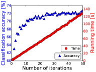
(a) Shortest-path kernel

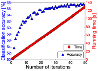
(b) Weisfeiler-Lehman subtree kernel

Figure 1: Influence of the number of iterations on the classification accuracy for HGK-SP and HGK-WL on the Enzymes data set.

VI Conclusion and Future Work

We have introduced the hash graph kernel framework which allows applying the various existing scalable and well-engineered kernels for graphs with discrete labels to graphs with continuous attributes. The derived kernels outperform other kernels tailored to attributed graphs in terms of running time without sacrificing classification accuracy.

Moreover, we showed that the hash graph kernel framework approximates implicit variants of the shortest-path and the Weisfeiler-Lehman subtree kernel with an arbitrary small error.

References

- [1] S. V. N. Vishwanathan, N. N. Schraudolph, R. Kondor and K. M. Borgwardt “Graph Kernels” In Journal of Machine Learning Research 11, 2010, pp. 1201–1242
- [2] M. Neumann, R. Garnett, C. Bauckhage and K. Kersting “Propagation kernels: Efficient graph kernels from propagated information” In Machine Learning 102.2, 2016, pp. 209–245
- [3] K. M. Borgwardt et al. “Protein function prediction via graph kernels.” In Bioinformatics 21 Suppl 1, 2005, pp. i47–i56
- [4] Z. Harchaoui and F. Bach “Image Classification with Segmentation Graph Kernels” In IEEE Conference on Computer Vision and Pattern Recognition, 2007, pp. 1–8
- [5] A. Feragen et al. “Scalable kernels for graphs with continuous attributes” Erratum available at http://image.diku.dk/aasa/papers/graphkernels_nips_erratum.pdf In Advances in Neural Information Processing System, 2013, pp. 216–224
- [6] N. Kriege and P. Mutzel “Subgraph Matching Kernels for Attributed Graphs” In Proceedings of the Twentieth International Conference on Machine Learning, 2012
- [7] F. Orsini, P. Frasconi and L. De Raedt “Graph Invariant Kernels” In Proceedings of the Twenty-fourth International Joint Conference on Artificial Intelligence, 2015, pp. 3756–3762
- [8] N. Kriege, M. Neumann, K. Kersting and M. Mutzel “Explicit versus Implicit Graph Feature Maps: A Computational Phase Transition for Walk Kernels” In 2014 IEEE International Conference on Data Mining, 2014, pp. 881–886
- [9] T. Joachims “Training Linear SVMs in Linear Time” In Proceedings of the Twelfth ACM SIGKDD International Conference on Knowledge Discovery and Data Mining, 2006, pp. 217–226
- [10] T. Gärtner, P. Flach and S. Wrobel “On Graph Kernels: Hardness Results and Efficient Alternatives” In Learning Theory and Kernel Machines, 2003, pp. 129–143
- [11] H. Kashima, K. Tsuda and A. Inokuchi “Marginalized Kernels Between Labeled Graphs” In Proceedings of the Twentieth International Conference on Machine Learning, 2003, pp. 321–328
- [12] U. Kang, H. Tong and J. Sun “Fast Random Walk Graph Kernel” In Proceedings of the 2012 SIAM International Conference on Data Mining, 2012, pp. 828–838
- [13] P. Mahé et al. “Extensions of marginalized graph kernels” In Proceedings of the Twenty-first International Conference on Machine Learning, 2004, pp. 552–559
- [14] J. Ramon and T. Gärtner “Expressivity versus Efficiency of Graph Kernels” In First International Workshop on Mining Graphs, Trees and Sequences, 2003
- [15] K. M. Borgwardt and H.-P. Kriegel “Shortest-path kernels on graphs” In Proceedings of the Fifth IEEE International Conference on Data Mining, 2005, pp. 74–81
- [16] N. Shervashidze et al. “Efficient Graphlet Kernels for Large Graph Comparison” In Proceedings of the Twelfth International Conference on Artificial Intelligence and Statistics, 2009, pp. 488–495
- [17] T. Horváth, T. Gärtner and S. Wrobel “Cyclic pattern kernels for predictive graph mining” In Proceedings of the Tenth ACM SIGKDD International Conference on Knowledge Discovery and Data Mining, 2004, pp. 158–167
- [18] S. Hido and H. Kashima “A Linear-Time Graph Kernel” In The Ninth IEEE International Conference on Data Mining, 2009, pp. 179–188
- [19] N. Shervashidze et al. “Weisfeiler-Lehman Graph Kernels” In Journal of Machine Learning Research 12, 2011, pp. 2539–2561
- [20] A. Rahimi and B. Recht “Random features for large-scale kernel machines” In Advances in Neural Information Processing Systems, 2008, pp. 1177–1184
- [21] A. Andoni “Nearest Neighbor Search: the Old, the New, and the Impossible”, 2009
- [22] M. Datar, N. Immorlica, P. Indyk and V. S. Mirrokni “Locality-sensitive hashing scheme based on -stable distributions” In Proceedings of the Twentieth Annual ACM Symposium on Computational Geometry, 2004, pp. 253–262
- [23] W. Hoeffding “Probability Inequalities for Sums of Bounded Random Variables” In Journal of the American Statistical Association 58.301, 1963, pp. 13–30
- [24] Isabelle Guyon “Design of experiments for the NIPS 2003 variable selection benchmark”, 2003 URL: http://clopinet.com/isabelle/Projects/NIPS2003/Slides/NIPS2003-Datasets.pdf
- [25] C.-C. Chang and C.-J. Lin “LIBSVM: A library for support vector machines” Software available at http://www.csie.ntu.edu.tw/~cjlin/libsvm In ACM Transactions on Intelligent Systems and Technology 2, 2011, pp. 27:1–27:27