Exploiting Universal Redundancy

Abstract

Fault tolerance is essential for building reliable services; however, it comes at the price of redundancy, mainly the “replication factor” and “diversity”. With the increasing reliance on Internet-based services, more machines (mainly servers) are needed to scale out, multiplied with the extra expense of replication. This paper revisits the very fundamentals of fault tolerance and presents “artificial redundancy”: a formal generalization of “exact copy” redundancy in which new sources of redundancy are exploited to build fault tolerant systems. On this concept, we show how to build “artificial replication” and design “artificial fault tolerance” (AFT). We discuss the properties of these new techniques showing that AFT extends current fault tolerant approaches to use other forms of redundancy aiming at reduced cost and high diversity.

I Introduction

Fault tolerance (FT) is the central pillar of reliable services [1, 2, 3, 4, 5]. A fault tolerant system must employ some form of redundancy Redundancy in space is often used against a specific pre-defined class of faults, like fail-stop, fail-recovery, Byzantine [1, 4], and employs a fault tolerant protocol that ensures the correctness of the system through replication and agreement techniques, e.g., TMR, consensus, failure detectors [6, 1, 7]. Unfortunately, these techniques are costly and their effectiveness are questionable due to the replication factor and diversity.

In particular, in order to tolerate $f$ faults, a FT protocol requires a minimum number of redundant components (i.e., replicas), called the replication factor, which is often $2f+1$ and can spans up to $5f+1$ in some fault models [3, 8, 9, 10]. The thorough reliance on Internet services nowadays amplifies these costs as more machines (either virtual of physical) are required to cope with the increasing demand on services; due to replication, this cost is multiplied by (at least) a factor of two or three. On the other hand, independence of failures between replicas is a major assumption for the correctness of FT protocols: a common fault among system replicas can bring them to fail unanimously, rendering the replication factor useless [11, 12, 13, 5]. This is usually mitigated by introducing some software and hardware diversity in the replicated components on different axes and levels [14, 15, 16, 17, 5, 18, 19, 20]. Although these approaches improve the FT of systems through diversity, they are costly and not always effective [11, 15, 5]. For instance, N-version programming [15, 1] introduces diversity into software through coding it in multiple versions by different independent teams and programming languages. In addition to its high cost in practice, it has been shown that dependency still exists since (1) developers often fall in the same mistakes and (2) as long as different versions originate from a common specification [11, 15]. Another interesting approach is proactive recovery between diverse obfuscated components that are generated to be semantically equivalent using a secret key [16, 17]; though interesting, it is only effective in transient failures and when the key is kept secret [14, 21]. BASE [5] introduces design diversity using Components Off-The-Shelf (COTS). The idea is to employ pre-existing diverse components that have similar behavior, and then write software wrappers to mimic the state machine behavior. Although this approach is promising, it is limited to the existence of COTS in various programming languages.

In this paper, we revisit the very fundamentals of fault tolerance and introduce artificial redundancy considering the “redundant information” inferred through the “action on a component” rather than the “component” itself: a component is artificially redundant to another one if there is a strong correlation between them, even if they are non similar in behavior or semantics. For example, two always opposite buffers $A=-B$ are artificially redundant since there is a perfect (though negative) correlation between them, as if they are exact copies. On the other hand, “the presence of ice” is artificially redundant, with some uncertainty, to “the atmospheric temperature is low” since they are strongly (but not perfectly) correlated.

Artificial replication can then be achieved by making an artificially redundant component an artificial replica, artira for short. The idea is to wrap the component by an adapter to code (resp., decode) the input (resp., output) of an artira as needed using component-specific (mathematical or probabilistic) transformation functions. Adapters are similar to the conformance wrappers used in BASE [5]; however, we apply it to completely independent, but correlated, components instead of those of similar behaviors allowing for some uncertainty (if needed). Artificial fault tolerance (AFT) is therefore achieved using replicas and artira, e.g., using voting or agreement, in a similar fashion to current FT protocols. When artira are perfectly correlated, existing FT protocols can be used with higher reliability due to the increased diversity of artiras. On the other hand, if artiras include some uncertainty (bounded or unbounded), new variants of AFT protocols are needed; in Section V, we only give some recommendations on how to build such protocols (due to size limitation).

Our work is complementary to existing FT models (in fact, AFT subsumes FT); and it is important for three main reasons: (1) it exploits new forms of redundancy to reduce the cost of replication that can, optionally, include some uncertainty; (2) it achieves equivalent or better tolerance to faults than classical FT being built on highly diverse components in terms of behavior, specification, providers, geographic location, etc.; and (3) it makes it possible to achieve lower levels of fault tolerance, e.g., detection, if some uncertainty is accepted by the application and when extra “exact copy” replicas do not exist or are not affordable; or if the service could not be easily replicated (e.g., redundant medical instruments, large scale social networks, etc.).

AFT may be criticized in two main ways. First, although AFT achieves high reliability in the case of perfect correlation, uncertainty in fault tolerance does not seem reasonable in other cases. Our argument is that, uncertainty even exists (under the hood) in current FT protocols; in fact, there is no evidence that FT protocols achieve 100% certainty due to dependence of failures [12]. On the other hand, the uncertainty we introduce here is agreed upon beforehand (e.g., in the SLA), and thus caution can be planned a priori. In addition, uncertainty in fault tolerance also do exist in literature as in [22, 7]. The second criticism is how practical is AFT. In fact, similar concepts have been studied and used in specific areas like automotive systems [23], clock synchronization [24, 25] and Byzantine approximate agreement [26], and we believe that these concepts can be generlized to a wider spectrum of distributed applications and services where even new forms of redundancy can be exploited as we do here. We show in Sections IV and VII that AFT can be applied to a large span of applications as in webservices, multithreading, HPC, etc. On the other hand, several applications can accept some uncertainty in FT to reduce the cost of replication or when additional replicas do not exist [27, 28].

To the best of our knowledge, this subject has not been studied in literature as we generlize here, and we believe that it is worth more investigation and empirical study in the future.

II Artificial Redundancy

II-A Notations

Consider a component $X$ that is associated with a set of possible actions in $A$. In general, an action can modify the state of X; however, for ease of presentation, we assume that actions are read-only and we explicitly mention writes when needed. We denote by $a(x)$ the output of an action $a\in A$ on a state $x\in X$, and by $X^{a}$ the range (i.e., output domain set) of $a$ on any state in X; we read this “X subject to action a”. Related, $X^{A}$ denotes the range of any action in A on any state in X, we read this “X subject to actions in A”. We also assume that $(X^{a},d)$ is a metric space with a defined distance $d$. We argue that any meaningful component output falls in this category. If $x$ is in a metric space $S$, a “closed ball” $N_{r}(x)$ of center $x$ and radius $r$ is the set: $N_{r}(x)=\{y:y\in S,d(x,y)\leq r\}$; then we say that $x$ is in the neighborhood of y.

II-B Artificial Redundancy

Definition 1 (Artificial Redundancy).

A component $X$ subject to action $a$ (i.e., $X^{a}$) is artificially redundant to component $Y$ subject to action $b$ (i.e., $Y^{b}$), denoted $X^{a}\curlyeqsucc Y^{b}$, iff there is a correlation $\zeta\in]0,1]$ between them.

The above definition is very relaxed as it makes any two components redundant to each other regardless of their behavior or semantics provided that there is a correlation between them. For instance, the atmospheric “temperature forecast” component on action $\mathsf{getTemperature()}$ is strongly correlated to the “snow forecast” component on action $\mathsf{isFalling()}$, and hence, they are artificially redundant. Although, artificial redundancy often makes sense when there is strong or perfect correlation (whether +ve or –ve), we do not explicitly mention the strength of correlation $\zeta$ to keep the definition general. The definition does not specify a correlation method to use; however, in general, any statistical correlation model can be used. Definition 1 is fine-grained to an individual action of a component (e.g., a function in a service API); however, in practice, services may not be equivalent (i.e., have different APIs); consequently, only parts of a service might be artificially redundant; this is captured by the following definition.

Definition 2 (Partial Artificial Redundancy).

A component $X$ subject to actions in $A$ ($X^{A}$), is partially artificially redundant to component $Y$ subject to actions in $B$ ($Y^{B}$) iff there exist at least one action $b\in B$ and a corresponding action $a\in A$ such that $X^{a}$ is artificially redundant to $Y^{b}$. In particular, if this is true $\forall b\in B$ (a surjection) then we say that $X$ is artificially redundant to $Y$, and denoted by $X^{A}\curlyeqprec Y^{B}$ or $X\curlyeqsucc Y$ when A=B.

Definition 2 governs the entire component when actions $A$ and $B$ are similar (e.g., if $X$ and $Y$ have the same API) as well as a subset of actions of the component (e.g., only some API functions are redundant). Artificial redundancy is often one-way relation as explained in Lemma 3.

Lemma 3 (Symmetry of Artificial Redundancy).

If $X^{a}\curlyeqsucc Y^{b}$ then $X^{a}\curlyeqprec Y^{b}$, therefore we say $X^{a}\approxeq Y^{b}$. To the contrary, if $X^{A}\curlyeqsucc Y^{B}$ then $X^{A}\curlyeqprec Y^{B}$ is not necessarily true.

Proof.

First part: If $X^{a}\curlyeqsucc Y^{b}$, then there exists a correlation between $X^{a}$ and $Y^{b}$; since correlation is symmetric by definition, then $X^{a}\curlyeqprec Y^{b}$ follows from Definition 1. Second part: follows from Definition 2 since there may exist an action $a^{\prime}\in A$ without any correlation to any action in $B$ (i.e., no surjection from $Y^{B}$ to $X^{A}$ exists). ∎

Since the goal of artificial redundancy is to establish (artificial) replication, we introduce the following lemma which makes this task easier.

Lemma 4 (Probabilistic Artificial Redundancy).

If $X^{a}\curlyeqsucc Y^{b}$ then $\exists\beta\in[0,1]$ and at least two predicates: $\mathcal{R}$ defined on $X^{a}$ and $\mathcal{Q}$ defined on $Y^{b}$ such that: $P(\mathcal{R}|Q)\geq\beta$.

Proof.

If $X^{a}\curlyeqsucc Y^{b}$ with correlation $\zeta$, then $\exists\beta\in[0,1]$ such that for any state $y\in Y^{b}$ there exists a corresponding state $x\in X^{a}$ with probability $\geq\beta$. Let the predicate $\mathcal{R}=$“$x$ exists” and $\mathcal{Q}=$“$y$ exists”, then the probability that $\mathcal{R}$ occurs given that $\mathcal{Q}$ occurs is $\geq\beta$. Therefore, $P(\mathcal{R}|Q)\geq\beta$. ∎

Lemma 4 says that if there are two correlated services, one can probably find two correlated predicates that are bounded (e.g., by $\beta$). This lemma will make it easier to establish correlations and lookup new redundancy forms in the next section.

III Artificial Replication

III-A Definitions

Artificial redundancy remains useless without the ability to transform artificially redundant components to replicas that can be used in practice. We make this possible by introducing artificial replication in Definition 5.

Definition 5 (Artificial Replication).

A component $X^{a}$ is said to be an artificial replica (artira for short) of $Y^{b}$ iff there exists $\alpha\in[0,1]$, $\epsilon\in Y^{b}$, and a transformation function $\mathcal{F}:X^{a}\longrightarrow Y^{b}$ such that $\forall y\in Y^{b},\exists x\in X^{a}$ such that $P\left(\hat{x}=\mathcal{F}(x)\in N_{\epsilon}(y)\right)\geq\alpha$. We denote this by: $X^{a}\in\mathcal{F}_{\epsilon}^{\alpha}(Y^{b})$.

Informally, this means that a component X (subject to an action $a$) is an artira of Y (subject to an action $b$) if we can find a function $\mathcal{F}$ such that for every state $y\in Y^{b}$ there is a state $x\in X^{a}$ such that $\mathcal{F}(x)$ is in the neighborhood of $y$ with some accuracy $\epsilon$ (i.e., the error is bounded) and certainty $\alpha$ (i.e., the bound is precise). An artira is defined in a triple $(\mathcal{F},\alpha,\epsilon)$ whose values must be defined a priori. Notice that, $X$ is an artira of $Y$ means that $Y$ is a reference replica and need not to be an artira of $X$. In principle, $\mathcal{F}$ is used to transform the output $a(x)$ of an action $a\in A$ on $x\in X$ to a value $\hat{x}=\mathcal{F}(a(x))\in Y^{b}$ such that $\hat{x}$ is close, with distance $\epsilon$, to some $y\in Y^{b}$ with certainty $\alpha$. The two metrics $\alpha$ and $\epsilon$ are strongly related and should be adjusted together: $\epsilon=0$ reflects 100% accuracy of $\mathcal{F}$ whereas $\alpha$ tells if this is correct all the time. Increasing $\epsilon$ makes the accuracy of $\mathcal{F}$ lower but with better certainty $\alpha$. We show in Section IV how can tuning $\alpha$ and $\epsilon$ bring interesting benefits.

III-B Building an Artira

Lemma 6.

Artificial redundancy is necessary, but not sufficient, for artificial replication.

Proof.

Necessary condition: consider the two predicates (i.e., events): $\mathcal{Q}=\{y=v|v\in Y^{b}\}$ and $\mathcal{R}=\{x=u\in{X^{a}}|\hat{x}=\mathcal{F}(u)\in N_{\epsilon}(y)\}$. From Definition 5, if $X^{a}$ is an artira of $Y^{b}$ then $\forall y\in Y^{b},\exists x\in X^{a}$ such that $P\left(\hat{x}\in N_{\epsilon}(y)\right)\geq\alpha$ for some $\alpha\in[0,1]$; hence, if $\mathcal{Q}$ occurs then $P(\mathcal{R})\geq\alpha$, i.e., $P(\mathcal{R}|Q)\geq\alpha$. Therefore, $X^{a}$ is artificially redundant to $Y^{b}$ as per Lemma 4.
Sufficient condition: trivial from Definition 5 since $\mathcal{F}$ does not always exist. ∎

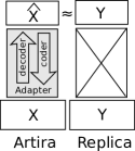
Figure 1: Artira vs. Replica.

Lemma 6 means that artiras can be built from artificially redundant components if the transformation $\mathcal{F}$ exists. We argue that such a transformation can often be defined if a strong correlation exists either by using accurate mathematical formulas or through using probabilistic prediction techniques (e.g., using Machine Learning), in which some uncertainty must be accepted by the application.

Building an artira $X^{a}$ of an existing replica $Y^{b}$ starts by defining the accepted accuracy $\epsilon$ and certainty $\alpha$ by the application. Then, if some strong correlation between $X^{a}$ and $Y^{b}$ exists, $X^{a}$ can likely be an artira of $Y^{b}$. Then, if a transformation $\mathcal{F}$ can be defined with some accuracy $\epsilon^{\prime}$ and certainty $\alpha^{\prime}$, $\epsilon^{\prime}$ and $\alpha^{\prime}$ are adjusted by incrementing $\epsilon^{\prime}$ to get a higher certainty $\alpha^{\prime}$. Finally, $X^{a}$ is accepted as an artira of $Y^{b}$ with the triple $(\mathcal{F},\alpha^{\prime},\epsilon^{\prime})$ if: $\alpha^{\prime}\geq\alpha$ and $\epsilon^{\prime}\leq\epsilon$. Building an artira $X^{A}$ of $Y^{B}$, i.e., considering multiple actions in $A$ and $B$, is done in a similar way by individually defining corresponding triples as $(\mathcal{F},\alpha,\epsilon)$.

Adapters. The transformation logic is then implemented in a wrapper on top of $X^{a}$, called adapter. Fig. 1 shows the architecture of an artira with an adapter versus a replica. An adapter can be state-full or stateless as conformance wrappers which were explained thoroughly in BASE [5], and therefore we skip this discussion here. Read operations use a decoder that implements $\mathcal{F}$ to transform outgoing values from the artira. Update operations, however, use a coder to write into the artira, which requires an inverse function $\mathcal{F}^{-1}$ to be defined. In this case, the parameters $\epsilon^{\prime}$ and $\alpha^{\prime}$ must be adjusted to consider the uncertainty of $\mathcal{F}^{-1}$ if it is not a perfect inverse of $\mathcal{F}$, since a read value will be affected twice by the uncertainty of both $\mathcal{F}$ and $\mathcal{F}^{-1}$. However, this is not required when $\mathcal{F}^{-1}$ is a perfect inverse (e.g., mathematical inverse function) of $\mathcal{F}$, since a value will be read exactly as it was previously written via the adapter (e.g., if $\mathcal{F}(x)=1/x$ and $\mathcal{F}^{-1}(x)=1/x$, then $\mathcal{F}(\mathcal{F}^{-1}(x))=x$). A reasonable cost must be paid while building an artira as discussed in Section V.

IV Artificial Redundancy and Replication Models

TABLE I: An abstraction of a simple component and the relation between two possible components.

Component:	$A_{i}$
$\mathop{\hbox{$\mathsf{val}$}}\nolimits$:	a value of any type.
$\mathop{\hbox{$\mathsf{expose}$}}\nolimits(\mathop{\hbox{$\mathsf{val}$}}\nolimits)$:	a read-only function that exposes the value of $\mathop{\hbox{$\mathsf{val}$}}\nolimits$.
$\mathop{\hbox{$\mathsf{modify}$}}\nolimits(\mathop{\hbox{$\mathsf{val}$}}\nolimits)$:	an update function that modifies the value of $\mathop{\hbox{$\mathsf{val}$}}\nolimits$.
Relation	$A_{i}$ and $A_{j}$
$\tau$:	Correlation threshold above which $\zeta\geq\tau$ is accepted.
$\mathcal{T}(\mathop{\hbox{$\mathsf{val}$}}\nolimits_{i},\mathop{\hbox{$\mathsf{val}$}}\nolimits_{j})$:	a relation upon which a transformation function $\mathcal{F}$ is defined.

We discuss the different artificial redundancy and replication models and their theoretical feasibility by considering a simple abstraction $A_{i}$ in Table I. More complex abstractions can intuitively be built on top of it, but this is enough to serve for explanation. $A_{i}$ is composed of a single value $\mathop{\hbox{$\mathsf{val}$}}\nolimits$ that represents the state of $A_{i}$; whereas $\mathop{\hbox{$\mathsf{expose}$}}\nolimits$ and $\mathop{\hbox{$\mathsf{modify}$}}\nolimits$ represent the read and write actions, respectively, that are accessible by any other abstraction $A_{j}$ (which may have different $\mathop{\hbox{$\mathsf{val}$}}\nolimits$ type and actions). We also represent the relation between $A_{i}$ and $A_{j}$ by the correlation threshold $\tau$ and the relation $\mathcal{T}$, where $\tau$ is the minimum correlation coefficient above which (inclusive) a service accepts components to be artificially redundant, whereas $\mathcal{T}$ materializes the correlation between two components be defining a transformation function $\mathcal{F}$ that may comprise some uncertainty as described. Based on this, we distinguish between interesting artificial replication and redundancy models summarized in Table II.

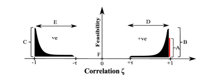
A: Exact copy	B: Perfect +ve correlation
C: Perfect -ve correlation	D: +ve correlation
E: -ve correlation	F: No correlation

Figure 2: Feasibility space of artificial redundancy.

TABLE II: The different models, settings, an use-cases of artificial replication and based on Table I.

Model	Correlation	Description	Use-case
PAR	EC	Exact Copy.	A replicated process having $\mathcal{T}=\{\mathcal{F}(\mathop{\hbox{$\mathsf{val}$}}\nolimits_{i})=\mathop{\hbox{$\mathsf{val}$}}\nolimits_{j}\}$.
	PC+	Perfect +ve Corr. $\tau=+1$	Two weather forecast processes where $A_{i}$ returns temperature in Celsius $\mathop{\hbox{$\mathsf{val}$}}\nolimits_{i}=C^{\circ}$ and $A_{j}$ in Fahrenheit $\mathop{\hbox{$\mathsf{val}$}}\nolimits_{j}=F^{\circ}$; then $\mathcal{T}=\{\mathcal{F}(\mathop{\hbox{$\mathsf{val}$}}\nolimits_{i})=(\mathop{\hbox{$\mathsf{val}$}}\nolimits_{j}-32)\times 5/9\}$.
	PC–	Perfect –ve Corr. $\tau=-1$	Two processes $A_{i}$ and $A_{j}$ having a shared buffer or token and using $\mathop{\hbox{$\mathsf{val}$}}\nolimits$ as a flag; thus $\mathcal{T}=\{\mathcal{F}(\mathop{\hbox{$\mathsf{val}$}}\nolimits_{i})=-\mathop{\hbox{$\mathsf{val}$}}\nolimits_{j}\}$.
SAR	BSC	Bounded Strong Corr. $|\tau|\geq 0.5$	Two medical diagnosis instruments: cardiac pulse meter $A_{i}$ and Electrocardiogram $A_{j}$ with sensors $\mathop{\hbox{$\mathsf{val}$}}\nolimits_{i}$ and $\mathop{\hbox{$\mathsf{val}$}}\nolimits_{j}$ (resp.); since both monitor heart activity, $\mathop{\hbox{$\mathsf{val}$}}\nolimits_{i}$ and $\mathop{\hbox{$\mathsf{val}$}}\nolimits_{j}$ are strongly correlated with some acceptable error $e$ bounded by $\delta$; therefore, $\mathcal{T}=\{\mathcal{F}(\mathop{\hbox{$\mathsf{val}$}}\nolimits_{i})=\mathop{\hbox{$\mathsf{val}$}}\nolimits_{j}\pm e|e\leq\delta\}$.
WAR	USC	Unbounded Strong Corr. $|\tau|\geq 0.5$	Two social-media profile recommender services that are statistically correlated but not bounded due to the tradeoff between accuracy and over-fitting. If the prediction function has an acceptable unbounded error $e$ and accuracy $p$; then $\mathcal{T}=\{\mathcal{F}(\mathop{\hbox{$\mathsf{val}$}}\nolimits_{i})=\mathop{\hbox{$\mathsf{svr}$}}\nolimits(\mathop{\hbox{$\mathsf{val}$}}\nolimits_{i})=\mathop{\hbox{$\mathsf{val}$}}\nolimits^{\prime}_{i}|P(|\mathop{\hbox{$\mathsf{val}$}}\nolimits^{\prime}_{i}-\mathop{\hbox{$\mathsf{val}$}}\nolimits_{j}|\leq\pm e)\geq p\}$.

For ease of presentation, we explain the different models and feasibility with the help of an “imaginary” feasibility spectrum depicted in Fig. 2. Since the ultimate goal is to build fault tolerant systems, which is often the basic defense layer in a service, critical services tend to adopt very strong correlation (e.g., $\tau$ is close to 1) and, gradually, fewer ones accept lower correlation coefficients. Therefore, our conjecture argues that the number of applications decreases (resp., increases) exponentially to $\tau$ (resp., $-\tau$) as the correlation coefficient $\zeta$ approaches zero. Notice that, theoretically, $\tau$ can be close to zero; however, it is merely meaningful only when $\tau>0.5$, i.e., when a strong correlation exists. Now, we discuss the different models.

IV-A Perfect Artificial Redundancy and Replication (PAR)

Perfect artificial redundancy refers to the case in which application FT requirements only accept perfect positive correlations between components, i.e., $\tau=\pm 1$; meaning that the information inferred by one component through the adapter is the exact information of the other with zero error. Consequently, PAR is the most interesting and desirable model to achieve fault tolerance. The feasibility is depicted in locations A, B, and C on Fig. 2. This is mapped to Table II. A refers to EC case which is the unique acceptable case in current FT. Artificial redundancy expands this case to use other redundancy sources as in PC+ (corr., B) and PC– (corr., C) with the same confidence as if they were exact replicas, as in A. From the perspective of artificial replication, this case refers to the configuration: $(\mathcal{F},\alpha=1,\epsilon=0)$. As shown in the use-cases of settings EC, PC+, and PC–, the function $\mathcal{F}$ transforms $\mathop{\hbox{$\mathsf{val}$}}\nolimits_{i}$ to $\mathop{\hbox{$\mathsf{val}$}}\nolimits_{j}$ without any error ($\epsilon=0$) and with 100% certainty ($\alpha=1$).

IV-B Strong Artificial Redundancy and Replication (SAR)

Strong artificial redundancy (SAR) refers to the case in which a small bounded error is tolerable as in BSC case in Table II. Though SAR is weaker than PAR, it is useful for some applications to avoid high costs of exact copies when high certainty is acceptable. Of course, such applications are much fewer than those of PAR; however, they do exist in practice as we explain in Section VII. In Fig. 2, this is depicted in the gradient color regions D and E. The dense color indicates more applications, showing that the more interesting cases are those when $\tau$ is closer to 1. In general, artificial replication is represented by $(\mathcal{F},\alpha\neq 1,\epsilon\neq 0)$ in SAR case; however, the parameters $\alpha$ and $\epsilon$ can be tuned since the inaccuracy is bounded. Thus, it may be suitable to increase $\epsilon$ so that a greater certainty $\alpha=1$ can be achieved and thus SAR becomes $(\mathcal{F},\alpha=1,\epsilon\neq 0)$. To explain this, consider the use-case in BSC settings in Table II. In this case, the medical instruments $A_{i}$ and $A_{j}$ can infer slightly different cardiac pulse $\mathop{\hbox{$\mathsf{val}$}}\nolimits$ that is bounded by $\delta$. Then, setting $\epsilon:=\delta$ such that $\alpha=1$ can be a good choice to get high certainty. This actually means that, the artificial replication is 100% accurate with an allowed error of $\delta$ cardiac pulses. We show how this is useful in Section V.

IV-C Weak Artificial Redundancy and Replication (WAR)

Weak artificial redundancy (WAR) refers to USC settings in Table II. It is similar to SAR in the correlation threshold $\tau$ and in feasibility (regions D and E in Fig. 2). However, in WAR, the transformation error could not be bounded, and thus certainty is never 100%. Consequently, weak artificial replication has the configuration: $(\mathcal{F},\alpha\neq 1,\epsilon\neq 0)$ where $\alpha$ and $\epsilon$ could not be tuned to have $\alpha=1$ (though tuning is possible in general). Note that, it is not always required to use artificial redundancy to make decisions, but to help making decisions like the use-case in USC settings. For instance, a fault raised by an artira can give an alert to do some “external” action (e.g., to explicitly verify correctness). Of course, WAR case is not suitable for sensitive applications that do not accept any uncertainty; however, it can be used in situations that are not critical to reduce the overhead of replication.

V Artificial Fault Tolerance (AFT)

V-A Definitions

Definition 7 (Artificial fault tolerance).

Artificial fault tolerance (AFT) is the approach used to achieve fault tolerance in a system of redundant components where at least one component is artificially redundant.

Definition 7 is general as it covers any sort of artificial redundancy. The use of redundancy is important since it is necessary to achieve fault tolerance [2]. Note that requiring at least one artificial redundant component means that there may exist other components that are not necessarily artificial (since artificial redundancy is not symmetric, as in Lemma 3).

In the rest of this paper, we focus on artificial replicas (artiras) as redundant components since it can be used to build AFT protocols. Due to size limitations, we address AFT protocols that can be used in active replication as in fault correction (or fault omission) through consensus [29, 3, 4, 1]. This is the dominant approach in practice since it gives the user an illusion that no faults occurred despite their actual presence. The main purpose of the protocols is to maintain a consistent system state and ensure that a single value is reported by the system to the client. Other forms of fault tolerance, like fault detection, can easily be derived from this study. In the following, we show how current FT protocols can be adjusted to support artiras, which are the building blocks of AFT protocols. We also discuss the properties of the system in this case and the differences to FT protocols.

V-B Recall FT Protocols

In order to cover a wide range of FT protocols, we focus on the common concepts across existing protocols and we explicitly address any protocol-specific properties.

Consider a system of $n$ nodes (e.g., replicas) where $f$ of them can be faulty (regardless of the fault model). In general, a client can send requests to one or more nodes and collect the received replies from one or more nodes too. To ensure correctness, consensus (or agreement) between nodes must be achieved. Many FT protocols assume network-partition faults which may split the nodes into two or more partitions [30, 4]. Therefore, they only require a quorum of nodes to reply correctly. To ensure correct Write and Read requests, the intersection of a Read quorum and a Write quorum must be correct (non-faulty). A common approach is to choose the quorum to be the majority of nodes (also called majority consensus), e.g., $\frac{n}{2}+1$; however, to support other protocols too, like 2PC and 3PC [31], we simply refer to this quorum as $q$. A FT protocol achieves consensus through three main phases:  Propose, Accept, and Learn.

• Propose: a value is proposed to agree upon.

• Accept: a proposed value is accepted by nodes if a quorum $q$ of nodes agree on it after following some message exchange pattern.

• Learn: the learner (often the requester) accepts the request if a quorum $q$ of replies match, and learns the matching value.

This notation is analogous to the phases used in the well-known protocols in literature as Paxos and BFT [30, 4]; however, it also covers other protocols regardless of which node is acting as proposer, acceptor, or learner, and how these phases are designed. We do not discuss message exchange patterns and delivery assumptions of an FT protocol since they are often the same as in AFT protocols (explained next). Committing a request is also protocol-dependent as it can occur in the Accept or Learn phases. In some protocols, Reads may not follow these phases except for the Learn phase in which a requester sends the request directly to all nodes and collects enough matching responses. In existing FT protocols, the matching logic $\mathop{\hbox{$\mathsf{ftmatch}$}}\nolimits$ to approve a request by the acceptors and the requester simply requires a quorum $q$ of responses $\mathsf{r_{k}}$ to be equal:

$$\mathsf{\mathop{\hbox{$\mathsf{ftmatch}$}}\nolimits=card(R_{q})\geq q;\ R_{q}=\{i\neq j~{}|~{}r_{i}=r_{j}\}}$$ (1)

Obviously, since all the quorum’s responses are equal, the committed value $\mathop{\hbox{$\mathsf{ftvalue}$}}\nolimits$ by the acceptors, as well as the learned value by the learner (or requester), is a single value which corresponds to any response in the quorum:

$$\mathsf{\mathop{\hbox{$\mathsf{ftvalue}$}}\nolimits=rand(r_{i})\ where\ i\in R_{q}}$$ (2)

V-C Designing AFT Protocols

Designing an AFT protocol starting from a FT protocol is reasonably not hard since the mechanics of the three phases is almost the same. The only sensitive parts are those which require deterministic behavior. Since in AFT at least one node will be an artira, this can incur some inaccuracy in the response returned by the decoder (as explained in Section III) which can induce indeterminism in some cases. This can require modifications in the three phases depending on the artificial replication model used. In general, the phases in an AFT protocol are defined as follows:

• Propose: one value is proposed to agree upon.

• Accept: one or more proposed values are accepted by nodes if a quorum $q$ of nodes agree on them after following some message exchange pattern.

• Learn: the learner (often the requester) accepts the request if a quorum $q$ of replies match with some uncertainty, and learns a chosen value according to some policy.

The uncertainty induced by the artiras require different matching logic to that in Eq. 1 as well since responses may not always be equal. For an AFT model defined by $F_{\epsilon}^{\alpha}$, the general matching criteria is as follows:

$$\mathsf{\mathop{\hbox{$\mathsf{aftmatch}$}}\nolimits=card(R^{\prime}_{q})\geq q;\ R^{\prime}_{q}=\{i\neq j|P(d(r_{i},r_{j})\leq\epsilon)\geq\alpha\}}$$ (3)

Equation 3 says that if the distance $d$ (defined in the metric space) between two responses is bounded by $\epsilon$ with probability $\alpha$ then these responses are considered matching. On the other hand, choosing a value by the requester in AFT follows an application-dependent $\mathop{\hbox{$\mathsf{policy}$}}\nolimits$ (e.g., priority, mean value, etc.):

$$\mathsf{\mathop{\hbox{$\mathsf{aftvalue}$}}\nolimits=\mathop{\hbox{$\mathsf{policy}$}}\nolimits(R^{\prime}_{q})}$$ (4)

Next, we discuss the properties of the system and how $\mathop{\hbox{$\mathsf{aftmatch}$}}\nolimits$ and $\mathop{\hbox{$\mathsf{aftvalue}$}}\nolimits$ change according to the replication model used (PAR, SAR, or WAR) together with the classical fault models.

V-C1 Benign Fault Models

A fault is considered “benign” if the corresponding faulty node either follows its correct specification or it crashes; examples are: crash-stop and crash-recovery, as in 2PC, 3PC, and Paxos [31, 30]. When only benign faults are assumed, we distinguish between the following cases:

PAR model

In the PAR replication model, an AFT protocol has the same design as a FT protocol. This is the most desired case since it is at least as robust as the existing FT case. (Additional robustness follows from the higher diversity of artiras). In PAR, the AFT system is defined by $\mathcal{F}_{\epsilon}^{\alpha}$ where $\epsilon=0$ and $\alpha=1$; thus, the adapter’s coding/decoding is perfect which makes the artiras deterministic, and equivalent to replicas in behavior. Therefore, the matching logic and the learned value become as follows:

$$\mathsf{\mathop{\hbox{$\mathsf{aftmatch}$}}\nolimits=card(R^{\prime\prime}_{q})\geq q;\ R^{\prime\prime}_{q}=\{i\neq j~{}|~{}d(r_{i},r_{j})=0\}}$$

$$\mathsf{\mathop{\hbox{$\mathsf{aftvalue}$}}\nolimits=rand(r_{i})\ where\ r_{i}\in R^{\prime\prime}_{q}}$$

Notice that the above equations are exactly equivalent to $\mathop{\hbox{$\mathsf{ftmatch}$}}\nolimits$ and $\mathop{\hbox{$\mathsf{ftvalue}$}}\nolimits$ in Eq. 3 and Eq. 4. This makes the AFT protocol phases (Propose, Accept, and Learn) exactly the same as those defined the FT case in Section V-B. Therefore, in PAR replication model, existing FT protocols can be used.

SAR model

In the SAR replication model, the AFT system is defined by $\mathcal{F}_{\epsilon}^{\alpha}$ where $\epsilon\neq 0$ and $\alpha=1$. This means that the error induced by the adapter’s coding/decoding is bounded by $\epsilon$ with probability $1$. Consequently, the matching logic becomes as follows:

$$\mathsf{\mathop{\hbox{$\mathsf{aftmatch}$}}\nolimits=card(R_{q})\geq q;R^{\prime\prime\prime}_{q}=\{i\neq j~{}|~{}d(r_{i},r_{j})\leq\epsilon\}}$$

Due to this bounded indeterminism, we distinguish between Read and Write requests. In Write requests, the proposer node, in the Propose phase, proposes a request value $req_{p}$. In the Accept phase, a quorum $q$ of nodes accept $req_{p}$ (regardless of the messaging patterns); the request is then committed by having all non-faulty nodes execute $req_{p}$ in the same order. However, since artiras are indeterministic, the local state of artiras can vary upon execution of $req_{p}$ within the bound defined by $\epsilon$. This does not affect the Learn phase since an ACK is enough to be sent to the requester.

A pedantic detail is to explicitly check if the bound $\epsilon$ is respected by having the proposer piggyback its state to the acceptors. This allows the acceptors to assert that $\mathop{\hbox{$\mathsf{aftmatch}$}}\nolimits$ is satisfied by comparing their local states to that of the proposer upon executing the request. In the protocols where a state value must be piggybacked along with the Write response to the requester, two options are possible to choose the learned value: (1) The proposer node that received the request from the requester can piggyback its state back to the requester after the Accept phase terminates successfully and the request has been executed by the proposer. This however limits the choices of the requester to the state of one node (the proposer in this case). This might be OK for some applications, but it might not be desired in others that prefer choosing a value according to a certain $\mathop{\hbox{$\mathsf{policy}$}}\nolimits$ (e.g., learn a value that corresponds to a replica instead of an artira). (2) All the states of all nodes are piggybacked to the requester in which case the latter can choose the preferred value according to its $\mathop{\hbox{$\mathsf{policy}$}}\nolimits$. This requires all nodes to share their states in the Accept phase. In particular, each node executes the request and replies back to the proposer or other nodes (depending on the message exchange pattern) with its state after execution. Since these states are possibly different, due to the uncertainty of artiras, the consensus problem is actually transformed to a multi-value or Vector consensus. Many consensus protocols of this class do exist in literature as Interactive Consistency (IC) Vectors [32], Approximate Agreement [26], and Vector Consensus (VC) [33]. In these approaches, the replicas, and artiras in our case, need to agree on a vector (or sub-vector) of correct proposed values instead of a single value. Using such consensus protocols guarantees that at least a quorum of $q$ values in the vector $V$ are accepted by acceptors. When $V$ is sent to the requester in the Learn phase, it can apply its $\mathop{\hbox{$\mathsf{policy}$}}\nolimits$ to choose a value from $V$.

Executing Read requests is similar to those of Write requests case. In some protocols, however, the requester directly sends its Read request to all nodes, which reply back with their local values to the client, without passing through the phases of the protocol described above. In this case, the received values can be treated as a vector, and then a value is chosen depending on the $\mathop{\hbox{$\mathsf{policy}$}}\nolimits$.

A $\mathop{\hbox{$\mathsf{policy}$}}\nolimits$ is application-dependent. In some cases, it is enough to choose: one value randomly, based on some criteria (like $max$ or $min$), or even an aggregate value (e.g., $sum$, $mean$). We show in Section VII that these policies are sometimes more interesting than choosing a single value.

WAR model

In the WAR replication model, $\epsilon\neq 0$ and $\alpha\neq 1$ since the error of the adapter coding/decoding could not be bounded. In this case, the matching policy remains the same as in Eq. 3. Consequently, it is not recommended to use this model for fault omissions since there is some probability to report a wrong value to the client. This can rather be used in fault detection when the application accepts some uncertainty and the service could not (or costly to) be easily replicated. We do not discuss this case as it is less interesting and we only discuss its possible applications in later sections.

V-C2 Non Benign Faults

A fault is said to be “non benign” if the corresponding faulty node may not behave according to its specification even without crashing. Well known examples are Byzantine and Rational faults [4, 34]. Since this can be seen as a form of indeterminism, we distinguish between the following cases.

PAR model

In PAR replication model ($F_{\epsilon}^{\alpha}$ where $\epsilon\neq 0$ and $\alpha=1$), an artira behaves exactly as a replica. Therefore, similar to the PAR case of benign faults above, there are no differences in the design of existing non benign FT protocols and those of AFT.

SAR model

In the SAR replication model, the inaccuracy of the adapter coding/decoding is bounded by $\epsilon\neq 0$. Therefore, the AFT protocol phases are different from those of an FT protocol in a similar way to the above discussion of benign FT protocols. However, since a non benign faulty node can have some indeterminism like an artira, this leverages important questions about how to distinguish between a correct behavior of an artira, due to uncertainty, and a faulty replica/artira as defined in the fault model like Byzantine, BAR, etc.  [35, 34]. This can cause problems under the hood since faulty nodes could skew the results of the consensus depending on the $\mathop{\hbox{$\mathsf{policy}$}}\nolimits$ used. For instance, if the $\mathop{\hbox{$\mathsf{policy}$}}\nolimits=\max$, then a Byzantine node can always try to reply with the maximum possible value that does not violate the bound $\epsilon$. Notice that even if this is within the acceptable limits of AFT, it may not be desired. We believe that this requires a dedicated research.

WAR model

This case is similar to that of the benign FT protocols described above.

VI The Cost of AFT

The discussion made in Sections I and V shows that the replication factor raises the cost of fault tolerance to many folds. This urges the majority of services to use FT techniques that require minimal number of replicas. Therefore, the norm is often to use the rule $n=2f+1$ and $n=3f+1$ for benign and non benign faults, respectively, and assuming $f=1$. Even in this best case, the cost of replication is two or three replicas. With the growth of computer-based services, the number of servers needed for replication will increase faster which imposes more cost on the service owner. This is not even consistent with the recent sustainability efforts of communities. The AFT approach we introduce here makes it possible to take advantage of existing resources to reduce the replication cost. This can stimulate designers to build their services keeping in mind their potential use as artiras.

However, there is some cost to pay due to: building artiras, new protocols, and uncertainty. For instance, as discussed in Section III, building artiras requires the existence of strongly correlated components. Although this depends on the application, it is costly to lookup synergies in a huge space of components, and thus it is recommended to designate a fairly small set of candidate components to verify correlations. This cost can also be reduced through using correlation tools as those used in Machine Learning and Data Analytics. This tradeoff is also required while implementing the adapter of an artira which shall not require a large investment in time and resources; otherwise, the cost will be similar to N-version programming [15]. Moreover, using artiras from other vendors can impose additional subscription and accessibility costs as in the cases of web-services (refer to Section VII). On the other hand, although AFT can use existing FT protocols as in the PAR model, other models require different protocol variants to consider the induced tolerable uncertainty. The cost of these protocols can be referred to the new forms of agreement (e.g., vector agreement), uncertainty handling, sending full replies instead of digests (since replies are not exact), etc. We argue that these costs are low compared to the benefits AFT brings in terms of using existing components and improving diversity; this also needs a dedicated empirical cost study in the future.

VII Feasibility and Applications

AFT Webservices

An interesting observation is that the web (e.g., web-services, crowdsourcing, BigData, etc.) contains lots of redundant information that is not being used in fault tolerance. For instance, the leading Web API directory in [36] shows that dozens of web-services exist in each API category (e.g., currency, weather, dictionaries, BigData, etc.). Given this, it would be interesting to exploit these redundant sources and use them as PAR artiras to design other more reliable service (rewarded by the increased diversity and distinct geographic locations of artiras). In addition, the SAR model can be used for webservices that can trade some bounded uncertainty for reduced cost. Moreover, if using web-services of different behaviors is possible (e.g., weather forecast and sea level elevation) more reliable webservices can be designed using the SAR and WAR models (if statistical correlations exist), provided that some uncertainty is accepted. We think that this can introduce a new business model in which webservices are provided to clients which in their turn can build more reliable webservices based on various ones. For instance, many weather forecast webservices are now available through the SOAP web programming model [37]. A more robust weather forecast webservice can be built, by using other webservices as artiras, and the new service is again sold to clients. Notice that the overhead of implementing such a webservice is low, using SOAP for example, and reduces the administrative cost of maintaining the whole system (since individual artira providers will take care of their webservices). The above concept can also be applied within the same company. For instance, SAR and WAR can be used through using two Google’s social media services, e.g., Youtube and Google+, as artiras to detect failures in recommender systems, e.g., through matching a user profile, interests, preferences, etc.

AFT in Distributed Programming

With the introduction of multicore systems, most programming languages support multithreading and multiprocessing which significantly increases the complexity of software designs. This makes software more prone to errors due to concurrency, shared resources, memory leaks, etc. Modern programming languages provide methods and techniques for error handling and processes recovery. For instance, Erlang allows processes to monitor each other for error handling [38]. If an exception is raised by one process, a linked trapping process can catch that exception and recover the failing process. The exception can comprise useful information about the reasons of the crash. The same concept can be used in AFT between processes by making some of them artiras to others (e.g., a supervisor parent process). In this way, processes can raise useful information that can be redundant to those in other processes even without failure and without necessarily using the exception. Following this approach, AFT can be used among different correlated processes and threads that share the same resources (drives, tokens, ports, folders etc.), e.g., as in NFS systems. Another example is to use AFT for Virtual Machines (like JVM) to detect faults as in a shared memory prefetching between correlated threads as in [39].

AFT by Design in HPC

High Performance Computing (HPC) has recently become a very hot area due to the high processing power required by Science, Social Network, and in general Big Data. In HPC, MapReduce is often used to break down a problem into Map and Reduce processes in a supercomputer, or simply a large number of processors [40]. Maps usually run in parallel over different processors and Reduce aggregates the final output emitted by Maps. Since it is costly to replicate the processes for better fault tolerance, it can be interesting to construct the problem in such a way that different processes can serve as artiras for others, even if they are different [41]. A simple example is the multiplication of huge matrices in which Map processes are assigned parts of a matrix like rows/columns/blocks. If there are patterns in the matrix (e.g., sorting), it is not difficult to detect a failure of a Map process if the values emitted by the adjacent Map processes are captured. Another option is to design the problem in a way to use processes as artiras, e.g., like using multi-level MapReduce steps [42]. In general, naturally redundant algorithms can intuitively be split into different processes that work in parallel in which they infer some redundant information (e.g., computing on the sub-trees of a binary tree) as described in [43].

Fault Detection

On the other hand, AFT can be used for fault detection (even in the WAR model). In fact, uncertainty and accuracy in failure detectors is well-studied in the literature; Failure Informers and Impact FD  [22, 7] are few examples. These works support our idea that fault tolerance can accept some uncertainty as in SAR and WAR models. Moreover, SAR and WAR can also be used for diagnosis. The BSC use-case in Table II is an example for detecting failed medical instruments. Similar applications can also accept some error like medical imaging [27], video streaming, self correcting applications (as genetic algorithms).

VIII Related Work

Von Neumann introduced the idea of redundancy in software by showing how reliable “organisms” can be synthesized from unreliable components via majority “organs” [44]. Most modern fault tolerance approaches used this concept through designing protocols with Active Replication as in [1, 29, 4, 3]. In order to tolerate $f$, faults, a number of extra components (i.e., replication factor) is required, based on $f$, with the assumption that replicas fail independently. In this paper, the AFT concept is based on artificial redundancy where replicas may not be exact-copies. This allows for other relaxed FT models that can be useful to reduce the cost of replication.

Fault tolerance protocols assume that replicas fail independently. To improve independence of failures, different forms of diversity can be introduced across different components on different axes and levels [14]: N-version programming [15], obfuscated software components [16], Components off-the-shelf (COTS) [5], various hardware [18], diverse OS [19], instruction sets [45], memory obfuscation [46], execution and compilation [21], etc. The most popular among these are N-version programming, “proactive recovery”, and using COTS to include design diversity to the system. N-version programming requires implementing a software by different independent teams which is very expensive [11, 13]. The second approach uses semantically equivalent generated (using a secret key) obfuscated components in proactive recovery fashion; this approach is only effective in “fast” failures and when the key is kept secret as described in [14, 21]. Finally, using COTS, as in BASE [5] is a promising approach as it uses already existing components of similar behaviors, which reduces the diversity cost (as in N-version programming). The approach uses conformance wrappers for components to achieve a similar behavior to state machines [29]. Our work generalizes this idea to use components of different behaviors, which has a larger application space and improved diversity. In addition, the logic and design of adapters in this paper is very similar to conformance wrappers in BASE.

Our idea is close to using diverse assistant systems in automotive systems [23] where a different system can take over when a critical system fails; however, we generalize this to span generic redundant system that can be used in distributed systems. On the other hand, clock synchronization [24, 25] and Byzantine approximate agreement [26] tried to strengthen the validity property through choosing approximate or average values. However, these works addressed systems where replicas (or clocks) are identical. Our work exploits the case where distributed componenets are different in behaviour and semantics; it looks up new redundancy forms even through opposite components in nature and functionallity, which ensures validity through using the “adapters”.

IX Concluding Remarks

This paper introduces a new form of artificial redundancy that is based on the correlations among components rather than on exact copies or similar behaviors. This allows to exploit new sorts of redundancy aiming at reducing the cost of replication and improving independence of failures. We described how to build artificial replicas, i.e., artiras, using artificial redundancy and explained the possible models depending on the correlations. Then, artificial fault tolerance (AFT) was introduced based on artiras instead of replicas, which induces some uncertainty in some cases. Our work is complementary to previous FT approaches and obviously does not replace them. AFT PAR model allows to use artiras in a similar fashion and certainty as conventional FT models use replicas, but with higher tolerance to faults due to the increased diversity by artiras. Other AFT SAR and WAR models can be used if the application tolerates some degree of uncertainty. In such cases, conventional FT protocols must be adjusted to include uncertainty. This imposes some cost as explained in Section V. We discussed the feasibility and applications (refer to Section VII) of our approach and explained that new business models can even be introduced on this concept. We beleive that is interesting to empirically study the tradeoffs between FT and AFT in terms of fault tolerance, efficiency, and cost in the future.

References

- [1] J. Gray and D. P. Siewiorek, “High-availability computer systems,” Computer, vol. 24, no. 9, pp. 39–48, Sep. 1991.
- [2] F. C. Gärtner, “Fundamentals of fault-tolerant distributed computing in asynchronous environments,” ACM Comput. Surv., vol. 31, no. 1, pp. 1–26, Mar. 1999.
- [3] T. D. Chandra, R. Griesemer, and J. Redstone, “Paxos made live: An engineering perspective,” in Proceedings of the Twenty-sixth Annual ACM Symposium on Principles of Distributed Computing, ser. PODC ’07. New York,NY,USA: ACM, 2007, pp. 398–407.
- [4] M. Castro and B. Liskov, “Practical byzantine fault tolerance,” in Proceedings of the Third Symposium on Operating Systems Design and Implementation, ser. OSDI ’99. Berkeley,CA,USA: USENIX Association, 1999, pp. 173–186.
- [5] M. Castro, R. Rodrigues, and B. Liskov, “Base: Using abstraction to improve fault tolerance,” ACM Trans. Comput. Syst., vol. 21, no. 3, pp. 236–269, Aug. 2003.
- [6] R. Lyons and W. Vanderkulk, “The use of triple-modular redundancy to improve computer reliability,” IBM Journal of Research and Development, vol. 6, no. 2, pp. 200–209, April 1962.
- [7] T. D. Chandra and S. Toueg, “Unreliable failure detectors for reliable distributed systems,” J. ACM, vol. 43, no. 2, pp. 225–267, Mar. 1996.
- [8] K. Shvachko, H. Kuang, S. Radia, and R. Chansler, “The hadoop distributed file system,” in Proceedings of the 2010 IEEE 26th Symposium on Mass Storage Systems and Technologies (MSST), ser. MSST ’10. Washington,DC,USA: IEEE Computer Society, 2010, pp. 1–10.
- [9] M. Abd-El-Malek, G. R. Ganger, G. R. Goodson, M. K. Reiter, and J. J. Wylie, “Fault-scalable byzantine fault-tolerant services,” SIGOPS Oper. Syst. Rev., vol. 39, no. 5, pp. 59–74, Oct. 2005.
- [10] R. Kotla, L. Alvisi, M. Dahlin, A. Clement, and E. Wong, “Zyzzyva: Speculative byzantine fault tolerance,” SIGOPS Oper. Syst. Rev., vol. 41, no. 6, pp. 45–58, Oct. 2007.
- [11] J. C. Knight and N. G. Leveson, “An experimental evaluation of the assumption of independence in multiversion programming,” IEEE Trans. Softw. Eng., vol. 12, no. 1, pp. 96–109, Jan. 1986.
- [12] D. E. Eckhardt and L. D. Lee, “A theoretical basis for the analysis of multiversion software subject to coincident errors,” IEEE Trans. Softw. Eng., vol. 11, no. 12, pp. 1511–1517, Dec. 1985.
- [13] D. E. Eckhardt, A. K. Caglayan, J. C. Knight, L. D. Lee, D. F. McAllister, M. A. Vouk, and J. J. P. Kelly, “An experimental evaluation of software redundancy as a strategy for improving reliability,” IEEE Trans. Softw. Eng., vol. 17, no. 7, pp. 692–702, Jul. 1991.
- [14] R. R. Obelheiro, A. N. Bessani, L. C. Lung, and M. Correia, “How practical are intrusion-tolerant distributed systems?” 2006.
- [15] L. Chen and A. Avizienis, “N-version programming: A fault-tolerance approach to reliability of software operation,” in Digest of Papers FTCS-8: Eighth Annual International Conference on Fault Tolerant Computing, 1978, pp. 3–9.
- [16] T. Roeder and F. B. Schneider, “Proactive obfuscation,” ACM Trans. Comput. Syst., vol. 28, no. 2, pp. 4:1–4:54, Jul. 2010.
- [17] F. B. Schneider and L. Zhou, “Distributed trust: Supporting fault-tolerance and attack-tolerance,” Cornell University, Tech. Rep., 2004.
- [18] R. Hughes, “A new approach to common cause failure,” Reliability Engineering, vol. 17, no. 3, pp. 211–236, 1987.
- [19] M. Garcia, A. Bessani, I. Gashi, N. Neves, and R. Obelheiro, “Os diversity for intrusion tolerance: Myth or reality?” in Dependable Systems Networks (DSN), 2011 IEEE/IFIP 41st International Conference on, June 2011, pp. 383–394.
- [20] A. Baumann, P. Barham, P.-E. Dagand, T. Harris, R. Isaacs, S. Peter, T. Roscoe, A. Schüpbach, and A. Singhania, “The multikernel: A new os architecture for scalable multicore systems,” in Proceedings of the ACM SIGOPS 22Nd Symposium on Operating Systems Principles, ser. SOSP ’09. New York, NY, USA: ACM, 2009, pp. 29–44.
- [21] B. Cox, D. Evans, A. Filipi, J. Rowanhill, W. Hu, J. Davidson, J. Knight, A. Nguyen-Tuong, and J. Hiser, “N-variant systems: A secretless framework for security through diversity,” in Proceedings of the 15th Conference on USENIX Security Symposium - Volume 15, ser. USENIX-SS’06. Berkeley,CA,USA: USENIX Association, 2006.
- [22] J. B. Leners, T. Gupta, M. K. Aguilera, and M. Walfish, “Improving availability in distributed systems with failure informers,” in Proceedings of the 10th USENIX Conference on Networked Systems Design and Implementation, ser. nsdi’13. Berkeley,CA,USA: USENIX Association, 2013, pp. 427–442. [Online]. Available: http://dl.acm.org/citation.cfm?id=2482626.2482667
- [23] W. Ren and R. W. Beard, Distributed consensus in multi-vehicle cooperative control. Springer, 2008.
- [24] L. Lamport and P. M. Melliar-Smith, “Synchronizing clocks in the presence of faults,” Journal of the ACM (JACM), vol. 32, no. 1, pp. 52–78, 1985.
- [25] S. R. Mahaney and F. B. Schneider, “Inexact agreement: accuracy, precision, and graceful degradation,” in Proceedings of the fourth annual ACM symposium on Principles of distributed computing. ACM, 1985, pp. 237–249.
- [26] D. Dolev, N. A. Lynch, S. S. Pinter, E. W. Stark, and W. E. Weihl, “Reaching approximate agreement in the presence of faults,” J. ACM, vol. 33, no. 3, pp. 499–516, May 1986.
- [27] J. Montagnat, V. Breton, and I. Magnin, “Partitionning medical image databases for content-based queries on a grid,” Methods of Information in Medicine, vol. 44, no. 2, pp. 154–160, 2005.
- [28] L. F. G. Sarmenta, “Sabotage-tolerance mechanisms for volunteer computing systems,” Future Gener. Comput. Syst., vol. 18, no. 4, pp. 561–572, Mar. 2002. [Online]. Available: http://dx.doi.org/10.1016/S0167-739X(01)00077-2
- [29] F. B. Schneider, “Implementing fault-tolerant services using the state machine approach: A tutorial,” ACM Comput. Surv., vol. 22, no. 4, pp. 299–319, Dec. 1990.
- [30] L. Lamport, “The part-time parliament,” ACM Trans. Comput. Syst., vol. 16, no. 2, pp. 133–169, May 1998.
- [31] P. A. Bernstein, V. Hadzilacos, and N. Goodman, Concurrency Control and Recovery in Database Systems. Boston, MA, USA: Addison-Wesley Longman Publishing Co., Inc., 1987.
- [32] M. Pease, R. Shostak, and L. Lamport, “Reaching agreement in the presence of faults,” J. ACM, vol. 27, no. 2, pp. 228–234, Apr. 1980.
- [33] M. Correia, N. F. Neves, and P. Veríssimo, “From consensus to atomic broadcast: Time-free byzantine-resistant protocols without signatures,” The Computer Journal, vol. 49, no. 1, pp. 82–96, 2006.
- [34] A. Aiyer, S., L. Alvisi, A. Clement, M. Dahlin, J.-P. Martin, and C. Porth, “Bar fault tolerance for cooperative services,” SIGOPS Oper. Syst. Rev., vol. 39, no. 5, pp. 45–58, Oct. 2005.
- [35] L. Lamport, R. Shostak, and M. Pease, “The byzantine generals problem,” ACM Trans. Program. Lang. Syst., vol. 4, no. 3, pp. 382–401, Jul. 1982.
- [36] ProgrammableWeb, “Programmableweb website,” 2015. [Online]. Available: http://www.programmableweb.com
- [37] F. Curbera, M. Duftler, R. Khalaf, W. Nagy, N. Mukhi, and S. Weerawarana, “Unraveling the web services web: an introduction to soap, wsdl, and uddi,” IEEE Internet computing, no. 2, pp. 86–93, 2002.
- [38] F. Cesarini and S. Thompson, Erlang programming. ” O’Reilly Media, Inc.”, 2009.
- [39] Y. Solihin, J. Lee, and J. Torrellas, “Using a user-level memory thread for correlation prefetching,” SIGARCH Comput. Archit. News, vol. 30, no. 2, pp. 171–182, May 2002.
- [40] J. Dean and S. Ghemawat, “Mapreduce: simplified data processing on large clusters,” Communications of the ACM, vol. 51, no. 1, pp. 107–113, 2008.
- [41] B. Schroeder, G. Gibson et al., “A large-scale study of failures in high-performance computing systems,” Dependable and Secure Computing, IEEE Transactions on, vol. 7, no. 4, pp. 337–350, 2010.
- [42] M. Hall, “Two-step matrix multiplication with hadoop,” 2013. [Online]. Available: http://magpiehall.com/two-step-matrix-multiplication-with-hadoop/
- [43] L. Laranjeira, M. Malek, and R. Jenevein, “On tolerating faults in naturally redundant algorithms,” in Reliable Distributed Systems,1991. Proceedings.,Tenth Symposium on, Sep 1991, pp. 118–127.
- [44] J. Von Neumann, “Probabilistic logics and synthesis of reliable organisms from unreliable components,” Automata Studies, p. 43–98, 1994.
- [45] G. S. Kc, A. D. Keromytis, and V. Prevelakis, “Countering code-injection attacks with instruction-set randomization,” in Proceedings of the 10th ACM Conference on Computer and Communications Security, ser. CCS ’03. New York,NY,USA: ACM, 2003, pp. 272–280.
- [46] J. Xu, Z. Kalbarczyk, and R. Iyer, “Transparent runtime randomization for security,” in Reliable Distributed Systems,2003. Proceedings. 22nd International Symposium on, Oct 2003, pp. 260–269.