Nonequilibrium diagrammatic technique for Hubbard Green functions

Abstract

We introduce diagrammatic technique for Hubbard nonequilibrium Green functions (NEGF). The formulation is an extension of equilibrium considerations for strongly correlated lattice models to description of current carrying molecular junctions. Within the technique intra-system interactions are taken into account exactly, while molecular coupling to contacts is used as a small parameter in perturbative expansion. We demonstrate the viability of the approach with numerical simulations for a generic junction model of quantum dot coupled to two electron reservoirs.

I Introduction

Using single molecules as electronic devices was originally suggested in a seminal paper by Aviram and Ratner Aviram and Ratner (1974). First experimental realization of a single molecule conductance junction was reported twenty years later Reed et al. (1997). Since then the field of molecular electronics experienced rapid development Ratner (2013); today molecular junctions are utilized as both nanoscale devices and convenient platforms for study of fundamental physical properties of matter at nanoscale van der Molen et al. (2013); Aradhya and Venkataraman (2013). Experimental advancements in measurements of junction responses (charge, spin, and energy fluxes; optical scattering; thermoelectric characteristics) to external perturbations (bias and gate voltages, temperature gradient, optical and voltage pulses) led to a surge in development of corresponding theoretical tools.

Molecular electronics is an interdisciplinary area of research combining condensed matter physics, statistical mechanics, nanoplasmonics, nonlinear optics, quantum chemistry, and engineering. Traditionally theoretical considerations of molecular junctions employ tools originally developed in high energy physics and successfully utilized in mesoscopic physics for description of transport in quantum dot junctions. In particular, the nonequilibrium Green function (NEGF) technique Kadanoff and Baym (1962); Keldysh (1965); Danielewicz (1984); Rammer and Smith (1986) is the usual choice in ab initio simulations. The quasiparticle (orbital or elementary excitations) basis employed in NEGF has many important advantages, from the ability to easily treat systems of realistic sizes to developed diagrammatic perturbation theory which allows to account for intra-molecular interactions within a controlled expansion in a small interaction parameter. Density functional theory (DFT) Parr and Yang (1989); Dreizler and Gross (1990) - also formulated in the basis of effective single particle orbitals - yields molecular electronic structure. The natural combination of the two approaches, the NEGF-DFT, was formulated Damle et al. (2002); Xue et al. (2002); Brandbyge et al. (2002) and successfully applied in many simulations where intra-molecular interaction (e.g., electron-phonon coupling in the off-resonant tunneling regime) is the smallest energy scale Sergueev et al. (2005); Frederiksen et al. (2007); Schmaus et al. (2011); Avriller and Frederiksen (2012).

As in any technique, the NEGF-DFT has its limitations; in particular, in treating strong intra-molecular interactions. The limitations are especially evident in the resonant tunneling regime (regime where the electron tunnels into one of the molecular orbitals), which is of particular importance for practical applications van der Molen et al. (2013): a large response of the molecular structure to external perturbation (e.g., negative differential resistance Chen et al. (1999); Rinkiö et al. (2010); Blum et al. (2005); Kiehl et al. (2006); Lörtscher et al. (2006); Wei et al. (2007); Wu et al. (2008), current induced chemistry Ho (2002); Seideman (2003), or switching Blum et al. (2005); van der Molen and Liljeroth (2010); Osorio et al. (2010); Komeda et al. (2011); Schirm et al. (2013)) is a requirement for constructing an effective molecular device. For example, even such a simple resonant tunneling phenomenon as Coulomb blockade requires special treatment by DFT; only recently developed hybrid functionals Baer and Neuhauser (2005); Livshits and Baer (2007); Refaely-Abramson et al. (2012); Liu et al. (2014) are capable of appropriate description of the effect. Note that the often utilized Landauer-DFT version of the NEGF-DFT may even lead to qualitative failures Baratz et al. (2013, 2014). We note in passing that NEGF-DFT (and NEGF-TDDFT) approaches have also fundamental limitations related to both foundations of (TD)DFT (utilization of Kohn-Sham orbitals as physical objects, non-uniqueness of the excited-state potentials, question of stability, and chaos of the mapping of densities on potentials, etc.) Gaudoin and Burke (2004); Baer (2008) and in combination of DFT with NEGF for transport description Bâldea (2016).

Figure 1: Sketch of a molecular junction. Nonequilibrium atomic limit utilizes basis of many-body states of an isolated molecule (thus accounting for intra-molecular interactions) while treating coupling between molecule and contacts within perturbation theory.

The difficulties mentioned above with NEGF-DFT led to the development of a nonequilibrium theory in which the system’s response to external perturbations is described using the many-body eigenstates of the isolated molecule (see Fig. 1). Such basis may be advantageous in theoretical description of a number of experiments Park et al. (2000); Wurtz et al. (2007); Repp et al. (2010); Natelson et al. (2013); Schulz et al. (2015); Wagner et al. (2015). It also facilitates the incorporation of the methods of quantum chemistry Yeganeh et al. (2009) and nonlinear optical spectroscopy Gao and Galperin (2016a) (usually applied to isolated molecules) into description of open nonequilibrium molecular systems. Contrary to the NEGF, where quadratic system-bath coupling is taken into account exactly while intra-system interactions are treated by perturbation theory, techniques utilizing many-body states of the system account for the intra-system interactions exactly while coupling to contacts is treated perturbatively. Such techniques are mostly applicable for molecules relatively weakly coupled to substrate(s). Similar to the equilibrium analog we coined this as the nonequilibrium atomic limit White et al. (2014a). We note that consequences of treating molecule and its coupling to electrodes at different level of theory were discussed in the literature Bâldea et al. (2010). Validation of such an approach and dependence of results on different partitioning schemes in realistic simulations is postponed for future research.

There are two flavors of Green function techniques capable of describing response of a nonequilibrium system coupled to environment (e.g., molecule coupled to contacts) utilizing the system’s many-body states: the pseudoparticle (PP) NEGF and the Hubbard NEGF. A simplified variant of the former - the slave boson technique - has been utilized to describe transport in junctions in seminal papers by Wingreen and Meir Wingreen and Meir (1994). Recent development of the dynamical mean field theory Aoki et al. (2014) renewed interest in the PP-NEGF Eckstein and Werner (2010); Oh et al. (2011). The methodology in its lowest (second) order in the system-bath coupling (the non-crossing approximation, NCA) was recently applied to describe transport and optical response in molecular junctions Oh et al. (2011); White and Galperin (2012); White et al. (2012, 2013, 2014b); Chen et al. (2016). Pseudoparticle Green functions (two-time correlation functions of creation and annihilation operators of many-body states of the system) can be viewed as a generalization of density matrix (which describes time-local correlation of many-body states). The methodology utilizes second quantization in the state space. As a result its formal structure is completely equivalent to the standard NEGF. However such formulation is possible only in an extended Hilbert space, whose physical subspace is defined by the normalization condition (sum of probabilities for the system to be in any of its states should be one) Gao and Galperin (2016a). The latter restriction is the main inconvenience of the method.

The Hubbard NEGF is formulated solely in physical Hilbert space. It utilizes Hubbard (or projection) operators

$$\hat{X}_{S_{1}S_{2}}\equiv\lvert S_{1}\rangle\langle S_{2}\rvert$$ (1)

on the states $\lvert S_{1,2}\rangle$ of the system. Below we distinguish between diagonal (e.g., pair of states containing same number of electrons) and non-diagonal operators. For the latter we introduce creation (e.g., number of electrons in state $\lvert S_{1}\rangle$ is bigger compared with $\lvert S_{2}\rangle$) and annihilation operators of Fermi (e.g., difference in number of electrons between the two states is odd) or Bose type. Central object of interest is the Hubbard Green function (two-time correlation functions of the Hubbard operators)

$$G_{(S_{1}S_{2}),(S_{3}S_{4})}(\tau,\tau^{\prime})\equiv-i\langle T_{c}\,\hat{X}_{S_{1}S_{2}}(\tau)\,\hat{X}_{S_{3}S_{4}}^{\dagger}(\tau^{\prime})\rangle$$ (2)

Here $\tau$ and $\tau^{\prime}$ are the Keldysh contour variables, $T_{c}$ is the contour ordering operator, and $\hat{X}_{S_{1}S_{2}}$ and $\hat{X}_{S_{3}S_{4}}$ are annihilation operators in the Heisenberg representation. Green functions (2) are most closely related to the usual NEGF. Indeed, while NEGF deals with correlations of elementary excitations (quasiparticles) $\hat{c}_{i}$,

$$G_{ij}(\tau,\tau^{\prime})=-i\langle T_{c}\,\hat{c}_{i}(\tau)\,\hat{c}_{j}^{\dagger}(\tau^{\prime})\rangle,$$ (3)

the Hubbard NEGF yields spectral decomposition of the excitations into underlying transitions between many-body states of the system, $\hat{c}_{i}=\sum_{S_{1},S_{2}}\langle S_{1}\rvert\hat{c}_{i}\lvert S_{2}\rangle\,\hat{X}_{S_{1}S_{2}}$, and considers correlations between pairs of such transitions. Thus, knowing the Hubbard NEGFs one always can reconstruct the NEGF. Introducing auxiliary fields, one can write the exact equation of motion for the Hubbard NEGF (2) in terms of the fields and their functional derivatives (see, e.g., Ref. Galperin et al. (2008) for details), and solve them approximately. For example, ignoring the auxiliary fields in the EOM corresponds to the first Hubbard approximation (HIA) Fransson (2010). The method was applied to transport problems in a number of publications Fransson et al. (2002, 2004); Fransson (2005); Sandalov and Nazmitdinov (2006, 2007); Galperin et al. (2008); Yeganeh et al. (2009).

While applicable to Green functions, the auxiliary field approach is less convenient in derivations of multi-time correlation functions. Such functions yield information on optical response Mukamel (1995) to classical radiation fields Gao and Galperin (2016b), fluctuation theorems, and counting statistics Esposito et al. (2009) of the system. A possible alternative is diagrammatic perturbation theory, which allows building controlled approximations for both Green (two-time) and multi-time correlation functions. Here we present a nonequilibrium diagrammatic technique for the Hubbard NEGF, and illustrate its viability within generic model simulations. The approach is an extension of equilibrium diagrammatic technique for Hubbard operators in lattice models Izyumov and Skryabin (1988); Ovchinnikov and Val’kov (2004) applied to nonequilibrium realm of molecular junctions. It can be considered as a Green function generalization of the real-time perturbation theory developed for density matrices Schoeller and Schön (1994); König et al. (1996); Schoeller (2000); Leijnse and Wegewijs (2008). As such it illustrates connection between Green function and density matrix methodologies. We note in passing that density matrix oriented formulations capable to provide efficient numerical solutions for time-local quantities are available in the literature. Jin et al. (2008); Härtle et al. (2013); Yan (2014); Ye et al. (2016); Yan et al. (2016)

In summary, presented formulation is first nonequilibrium diagrammatic technique applicable to multi-time correlation functions of Hubbard operators. Contrary to standard diagrammatic techniques it utilizes system-bath coupling as a small parameter of expansion with intra-system interactions taken into account exactly. At the same time (similar to standard diagrammatic techniques) diagrams can be analyzed and particular subsets responsible for a physical process of interest retained. Compared to PP-NEGF (similar perturbative expansion) the current technique is formulated solely in the physical Hilbert space, which makes it potentially advantageous in formulation of, e.g., the full counting statistics for interacting systems. Finally, being much lighter than numerically exact methods the approach can be utilized in first principles simulations of realistic systems.

The structure of the paper is the following: Section II introduces general diagrammatic rules for the Hubbard NEGF. We specialize to generic model of a quantum dot junction in Section III. Section IV presents numerical simulations; where possible (in noninteracting case) we compare the perturbation theory to exact results. Section V concludes.

II Diagrammatic technique for Hubbard NEGF

Diagrammatic technique for NEGF is based on the Wick’s theorem Fetter and Walecka (1971) which relies on (anti)commutation relations for creation and annihilation (Fermi) Bose operators, $[\hat{c}_{i};\hat{c}^{\dagger}_{j}]_{\pm}=\delta_{i,j}$. Similarly one has to consider (anti)commutations of Hubbard operators for a transition $m=(S_{1},S_{2})$ between two many-body states being of a (Fermi) Bose type. The corresponding (anti)commutators for the Hubbard operators are

$$\left[\hat{X}_{S_{1}S_{2}};\hat{X}_{S_{3}S_{4}}^{\dagger}\right]_{\pm}=\delta_{S_{2},S_{4}}\hat{X}_{S_{1}S_{3}}\pm\delta_{S_{1},S_{3}}\hat{X}_{S_{4}S_{2}}$$ (4)

where the plus sign is taken if both $\hat{X}_{S_{1}S_{2}}$ and $\hat{X}_{S_{3}S_{4}}$ are fermionic Hubbard Operators and the minus sign otherwise. A crucial difference is appearance of an operator (contrary to number in quasiparticle case) in the right side of (4). Nevertheless a variant of the Wick’s theorem was developed for lattice models at equilibrium and corresponding diagrammatic techniques were formulated and applied to studies of strongly correlated magnetically ordered systems Izyumov and Skryabin (1988); Ovchinnikov and Val’kov (2004). The goal of this paper is to adapt the methodology to nonequilibrium realm of current carrying molecular junctions.

We consider generic model of a junction consisting of a molecule $M$ coupled to two contacts $L$ and $R$ each characterized by its own electrochemical potential $\mu_{L,R}$ and temperature $T_{L,R}$

$$\hat{H}=\hat{H}_{M}+\sum_{K=L,R}\left(\hat{H}_{K}+\hat{V}_{MK}\right)$$ (5)

Here $\hat{H}_{M}$ is Hamiltonian of an isolated molecule which we represent in the basis of many-body states $\{\lvert S\rangle\}$ of the the molecule. $\hat{H}_{K}$ describes reservoir of free electrons and $\hat{V}_{MK}$ couples the two subsystems. Explicit expressions are

$$\hat{H}_{M}= \sum_{S}E_{S}\hat{X}_{SS}$$ (6)

$$\hat{H}_{K}= \sum_{k\in K}\varepsilon_{k}\hat{c}_{k}^{\dagger}\hat{c}_{k}$$ (7)

$$\hat{V}_{MK}= \sum_{k\in K}\sum_{m\in M}\left(V_{km}\hat{c}_{k}^{\dagger}\hat{X}_{m}+H.c.\right),$$ (8)

where $E_{S}$ are energies of the many-body states, $\hat{X}_{SS}$ are states projection operators, $\hat{c}_{k}^{\dagger}$ ($\hat{c}_{k}$) is second quantization creation (annihilation) operator for an electron in level $k$ of contacts, and $m$ are single electron (Fermi type) transitions between pairs of molecular states. Below we consider expansion in the molecule-contact(s) coupling $\hat{V}=\sum_{K=L,R}\hat{V}_{MK}$.

We consider the Hubbard Green function defined on the Keldysh contour, Eq. (2). A multi-time correlation function can be treated similarly. Following the usual procedure we transfer to the interaction representation with respect to $\hat{H}_{0}=\hat{H}_{M}+\sum_{K=L,R}\hat{H}_{K}$ and expand the scattering operator $\hat{S}=\exp[-i\int_{c}d\tau\,\hat{V}(\tau)]$ (here and below operators are in the interaction picture) in Taylor series. This leads to

$$G_{(S_{1}S_{2}),(S_{3}S_{4})}(\tau,\tau^{\prime})=\sum_{n=0}^{\infty}\frac{(-i)^{n+1}}{n!}\int_{c}d\tau_{1}\ldots\int_{c}d\tau_{n}$$

$$\qquad\qquad\langle T_{c}\,\hat{X}_{S_{1}S_{2}}(\tau)\,\hat{X}_{S_{3}S_{4}}^{\dagger}(\tau^{\prime})\,\hat{V}(\tau_{1})\ldots\hat{V}(\tau_{n})\rangle_{0}$$ (9)

Subscript $0$ indicates that evolution in each term of the expansion is governed by the Hamiltonian $\hat{H}_{0}$ representing uncoupled molecule and contacts. In the usual spirit of NEGF technique we assume that molecule and contacts (originally decoupled) are connected at time $t\to-\infty$, and that original (before coupling) state of the system is a direct product of states of its parts, $\hat{\rho}_{0}=\hat{\rho}^{L}_{0}\otimes\hat{\rho}^{M}_{0}\otimes\hat{\rho}^{R}_{0}$. Thus quantum mechanical and statistical average, $\langle\ldots\rangle_{0}\equiv\mbox{Tr}[\ldots\hat{\rho}_{0}]$, in (II) can be splitted into the product of averages of molecular Hubbard operators and contact quasiparticle operators. The latter satisfy the usual Wick’s theorem Fetter and Walecka (1971) and thus can be represented as the sum of all possible products of pair correlation functions thus yielding products of molecular self-energies due to coupling to the contacts

$$\sigma^{K}_{mm^{\prime}}(\tau,\tau^{\prime})=\sum_{k\in K}V_{mk}\,g_{k}(\tau,\tau^{\prime})\,V_{km^{\prime}}$$ (10)

where $g_{k}(\tau,\tau^{\prime})\equiv-i\langle T_{c}\,\hat{c}_{k}(\tau)\,\hat{c}_{k}^{\dagger}(\tau^{\prime})\rangle$ is NEGF of free electron in level $k$ of contact $K$.

To evaluate the average of Hubbard operators we make two additional assumptions: 1. originally (at $t\to-\infty$) molecule was in thermal equilibrium and 2. after coupling to the contacts the system reached steady-state, i.e. memory of initial state was lost. The latter is a usual assumption within the NEGF, and thus the former is unimportant for long time behavior of the system. Choice of thermal equilibrium as initial condition for the molecule allows employing diagrammatic technique of Refs. Izyumov and Skryabin (1988); Ovchinnikov and Val’kov (2004) for evaluation of the average of Hubbard (molecular) operators. Because the (anti)commutator of two Hubbard operators is an operator, Eq. (4), the Wick’s theorem for Hubbard operators differs from its standard quasiparticle analog. First one distinguishes between non-diagonal (e.g., transition $(S_{1},S_{2})$ with states $\lvert S_{1}\rangle$ and $\lvert S_{2}\rangle$ different by a number of electrons) and diagonal Hubbard operators. Then pair contractions in a multi-time correlation function are created starting from one chosen non-diagonal operator (usually of annihilation type, i.e. such that number of electrons in state $\lvert S_{1}\rangle$ is less than the number in $\lvert S_{2}\rangle$) and continue sequentially following a set of rules regarding choice of a non-diagonal operator to start contraction at every step of the procedure. It is important to note that diagrammatic rules for contraction of Hubbard operators are not unique, that is the same correlation function can be formally written in several different (formally equivalent) ways depending on choice of a system of priorities for the operators Izyumov and Skryabin (1988). Another approach utilizes a principle of topological continuity: each next contraction starts from the operator obtained in the previous contraction step, if the operator is non-diagonal; otherwise contraction starts from a non-diagonal operator connected to the already contracted part by interaction line Ovchinnikov and Val’kov (2004). The latter choice allows to formulate the most general form of diagrammatic rules, however resulting diagrams are hard to analyze in terms of which physical processes they represent. In our analysis we will use a mixture of the two traditional choices.

Next we introduce the contraction rules for the diagrammatic technique

1. Contraction starts from the entrance point. In the Hubbard Green function (2) operator $\hat{X}_{S_{1}S_{2}}(\tau)$ is the entrance point, while operator $\hat{X}_{S_{3}S_{4}}^{\dagger}(\tau^{\prime})$ is the exit point. For a multi-time correlation function one can have several entrance (annihilation operator) and exit (creation operator) points; in this case contractions can start from any entrance point.

2. An annihilation operator resulting from $k$th contraction is the starting point of $(k+1)$th contraction.

3. If result of $k$th contraction is not an annihilation operator, then we chose an annihilation operator connected to the contracted part by interaction line as the starting point of $(k+1)$th contraction. Note that in our case interaction is self-energy due to coupling to contacts, Eq. (10).

4. If neither 2, nor 3 is possible, then $(k+1)$th contraction starts from one of unconnected annihilation operators chosen in accordance with accepted system of priorities (see Section III for details).

5. Single contraction from operator $\hat{X}_{m_{1}}$ to operator $\hat{X}_{m_{2}}$ (where $m_{i}$ is an index for a pair of states) is

   $$\contraction{\langle T_{c}\ldots}{\hat{X}}{{}_{m_{2}}(\tau_{2})\dots}{\hat{X}}\langle T_{c}\ldots\hat{X}_{m_{2}}(\tau_{2})\ldots\hat{X}_{m_{1}}(\tau_{1})\ldots\rangle_{0}=$$ (11)

   $$\quad(-1)^{P}ig^{(0)}_{m_{1}}(\tau_{1},\tau_{2})\langle\ldots[\hat{X}_{m_{1}};\hat{X}_{m_{2}}]_{\pm}(\tau_{2})\ldots\rangle_{0}$$

   Here $g^{(0)}_{m_{1}}(\tau_{1},\tau_{2})$ is zero order (in the absence of molecule-contacts coupling) Green function and $[\hat{X}_{m_{1}};\hat{X}_{m_{2}}]_{\pm}$ is operator of spectral weight defined in Eq. (4). $P$ depends on the type of the operator $\hat{X}_{m_{1}}$: for Bose type $P=0$; for Fermi type $P$ is the number of permutations of $\hat{X}_{m_{1}}$ with other Fermi operators in the correlation function of transition from original place of $\hat{X}_{m_{1}}$ to position in front of $\hat{X}_{m_{2}}$. Note that zero order Green function of Hubbard operators $G^{(0)}_{m_{1}}(\tau_{1},\tau_{2})$ differs from $g^{(0)}_{m_{1}}(\tau_{1},\tau_{2})$ by the spectral weight factor: $G^{(0)}_{m_{1}}(\tau_{1},\tau_{2})=g^{(0)}_{m_{1}}(\tau_{1},\tau_{2})\langle[\hat{X}_{m_{1}};\hat{X}_{m_{1}}]_{\pm}\rangle_{0}$ (the latter is called Green function Izyumov and Skryabin (1988), propagator Ovchinnikov and Val’kov (2004), or locator Fransson (2010) in the literature).

6. The sequence of contractions continues until all operators remaining in the correlation function are diagonal. Separate expansion should be constructed for these correlation functions.

7. Only connected diagrams are retained in the expansion.

8. After expansion to desired order of the coupling is finished the diagrams are dressed in complete analogy with the standard diagrammatic techniques.

In the resulting diagrams one can distinguish three types of contributions:

1. Self-energy contributions $\Sigma(\tau,\tau^{\prime})$ - irreducible (those which cannot be cut by one Green function line) parts of diagrams connected to the entrance and exit points, respectively operators $\hat{X}_{S_{1}S_{2}}(\tau)$ and $\hat{X}_{S_{3}S_{4}}^{\dagger}(\tau^{\prime})$ in Eq. (2), by Green function lines.

2. Spectral weight contributions $F(\tau)$ - parts of diagrams where entrance and exit points are connected by single Green function line.

3. Vertex contributions $\Delta(\tau,\tau^{\prime})$ - parts of diagrams connected to the entrance (but not exit) point by single Green function line.

The sum of the spectral weight and the vertex diagrams, $P(\tau,\tau^{\prime})=\delta(\tau,\tau^{\prime})F(\tau)+\Delta(\tau,\tau^{\prime})$, is called the strength operator Ovchinnikov and Val’kov (2004).

Figure 2: Graphical representation of the modified Dyson equation, Eqs. (12)-(13). Directed single solid line represents zero order Green function $g^{(0)}$, directed double line stands for the dressed Green function $g$, spectral weight $F$ is indicated with the circle, and vertex $\Delta$ with triangle. Semi-circle represents the strength operator $P$.

Expansion series can be resumed into a modified Dyson type equation

$$G_{mm^{\prime}}(\tau,\tau^{\prime})= \sum_{m_{1}}\int_{c}d\tau_{1}\,g_{mm_{1}}(\tau,\tau_{1})\,P_{m_{1}m^{\prime}}(\tau_{1},\tau^{\prime})$$ (12)

$$g_{mm^{\prime}}(\tau,\tau^{\prime})= g^{(0)}_{mm^{\prime}}(\tau,\tau^{\prime})+\sum_{m_{1},m_{2}}\int_{c}d\tau_{1}\int_{c}d\tau_{2}\,$$ (13)

$$g^{(0)}_{mm_{1}}(\tau,\tau_{1})\,\Sigma_{m_{1}m_{2}}(\tau_{1},\tau_{2})\,g_{m_{2}m^{\prime}}(\tau_{2},\tau^{\prime})$$

Also here indices $m$ indicate single-electron transitions between many-body states of the system. Graphical representation of the equations is shown in Fig. 2. Like the Dyson equation of the standard NEGF, Eqs. (12)-(13) are exact; their form reflects resummation of all the diagrams in perturbative expansion. Similar to the Dyson equation, where the approximation enters via a particular form of the self-energy, Eqs. (12)-(13) become approximate due to particular forms of the self-energy $\Sigma$ and strength operator $P$.

Note that similar structure of Green function (without vertex contribution) was obtained within equation-of-motion approach for retarded projection of the usual Green function, Eq. (3), in Ref. Haug and Jauho (2008); nonequilibrium version was derived in Ref. Galperin et al. (2007). Note also that Eqs. (12)-(13) are similar to those obtained within auxiliary fields approach Fransson (2010). However, contrary to the auxiliary fields approach to Hubbard NEGF diagrammatic formulation yields a clear procedure of perturbative accounting for the system-bath coupling, which is applicable also to multi-time correlation functions. In particular, already at second order in the coupling the diagrammatic technique yields vertex contribution, which is shown below to be crucial for both accuracy of the results and the very ability to predict co- and pair-tunneling in junctions.

III Quantum dot model

We now specify to a quantum dot junction. Molecular (quantum dot) subspace is spanned by four many-body states states $\lvert S\rangle$ ($S\in\{0,a,b,2\}$) of the following second quantized form

$$\lvert 0\rangle\equiv\lvert 0,0\rangle\quad\lvert a\rangle\equiv\lvert 1,0\rangle\quad\lvert b\rangle\equiv\lvert 0,1\rangle\quad\lvert 2\rangle\equiv\lvert 1,1\rangle$$ (14)

Energies of the states are $E_{0}=0$, $E_{a}=\varepsilon_{a}$, $E_{b}=\varepsilon_{b}$, and $E_{2}=\varepsilon_{a}+\varepsilon_{b}+U$, respectively. There are four Fermi type transitions $m\in\{1,2,3,4\}$ in the model corresponding to charge transfer between molecule and contacts

$$1.~{}\lvert 0\rangle\langle a\rvert\quad 2.~{}\lvert b\rangle\langle 2\rvert\quad 3.~{}\lvert 0\rangle\langle b\rvert\quad 4.~{}\lvert a\rangle\langle 2\rvert$$ (15)

Figure 3: Non-dressed diagrams up to second order in molecule-contacts coupling for Fermi Green function $G_{mm^{\prime}}$, Eq. (12), contributing to the spectral weight $F$ (circle, top panel), vertex $\Delta$ (triangle, middle panel), and self-energy $\Sigma$ (bottom panel). Solid line represents Fermi type Green function $g^{(0)}_{m}$, wavy line is the interaction (10), dashed line represents Bose type Green function for two-particle scattering $d^{(0)}_{02}$, and oval stands for the correlation function $C^{(0)}$.

Performing expansion up to second order in molecular coupling to contacts for the Hubbard Green function (2) and evaluating contractions following the rules discussed above leads to the set of diagrams presented in Fig. 3. Diagrams for the spectral weight $F_{mm^{\prime}}(\tau)$ (top panel in Fig. 3) can be disregarded, because the latter is related to lesser and greater projections of the Hubbard Green functions

$$F_{mm^{\prime}}(t)\equiv\langle\{\hat{X}_{m}(t);\hat{X}_{m^{\prime}}^{\dagger}(t)\}\rangle=iG_{mm^{\prime}}^{>}(t,t)-iG_{mm^{\prime}}^{<}(t,t)$$ (16)

Dressed versions of contributions to the vertex and self-energy (middle and bottom panels of Fig. 3, respectively) are

$$\Delta_{mm^{\prime}}(\tau,\tau^{\prime})=\sum_{m_{1},m_{2}}\int_{c}d\tau_{1}$$ (17)

$$\quad\bigg{(}i(-1)^{m^{\prime}}d_{02}(\tau,\tau^{\prime})\,g_{\bar{m}^{\prime}m_{2}}(\tau^{\prime},\tau_{1})\,F_{m_{2}m_{1}}(t_{1})\,\sigma_{m_{1}\bar{m}}(\tau_{1},\tau)$$

$$\quad+C_{mm_{1},m_{2}m^{\prime}}(\tau,\tau^{\prime})\,\sigma_{m_{1}m3}(\tau,\tau_{1})\,g_{m_{3}m_{2}}(\tau_{1},\tau^{\prime})\bigg{)}$$

$$\Sigma_{mm^{\prime}}(\tau,\tau^{\prime})=\sum_{m_{1}}F_{mm_{1}}(t)\,\sigma_{m_{1}m^{\prime}}(\tau,\tau^{\prime})$$ (18)

$$\quad+i\delta(\tau,\tau^{\prime})\sum_{m_{1},m_{2},m_{3}}\eta(m_{3},mm_{1})\,\delta_{\gamma(m_{3},mm_{1}),m^{\prime}}$$

$$\qquad\qquad\qquad\times\int_{c}d\tau_{1}\,\sigma_{m_{1}m_{2}}(\tau,\tau_{1})\,G_{m_{2}m_{3}}(\tau_{1},\tau)$$

$$\quad+i(-1)^{m^{\prime}}d_{02}(\tau,\tau^{\prime})\,\sigma_{\bar{m}^{\prime}\bar{m}}(\tau^{\prime},\tau)$$

Here $\bar{m}=3-m$, $\eta(m,m_{1}m_{2})$ and $\gamma(m,m_{1}m_{2})$ are defined in (24) and (25), $d_{02}(\tau,\tau^{\prime})$ is Green function (locator) corresponding to two-electron Hubbard Green function

$$D_{02}(\tau,\tau^{\prime})=-i\langle T_{c}\,\hat{X}_{02}(\tau)\,\hat{X}_{02}^{\dagger}(\tau^{\prime})\rangle,$$ (19)

and

$$C_{m_{1}m_{2},m_{3}m_{4}}(\tau,\tau^{\prime})=\langle T_{c}\,\delta\hat{F}_{m_{1}m_{2}}(\tau)\,\delta\hat{F}_{m_{3}m_{4}}(\tau^{\prime})\rangle$$ (20)

($\delta\hat{F}\equiv\hat{F}-\langle\hat{F}\rangle$) is the correlation function. In derivation of Eqs. (17)-(18) we utilized commutation relations presented in Appendix A. Fourth order expressions are written in Appendix B. Similarly, diagrammatic expansions are performed for the functions (19) and (20). We discuss them in Appendices C and D, respectively.

Comparing with previous works on the Hubbard NEGF Galperin et al. (2008); Fransson (2010); Fransson et al. (2002, 2004); Fransson (2005); Sandalov and Nazmitdinov (2006, 2007) we note that considerations there were restricted to the first and (sometimes also) second diagram in the bottom panel of Fig. 3 - correspondingly first Hubbard (HIA) and one-loop approximations. Below we show that other second order diagrams are also important. In particular, second diagram in the middle panel of Fig. 3 is crucial in obtaining better approximations of exact results in the single electron tunneling regime and is an inherent part of description of cotunneling in junctions, while first diagram in the middle and last diagram in the bottom panels of Fig. 3 are responsible for pair electron tunneling. We also note that contrary to a common perception Pedersen et al. (2009) HIA is not a lowest order approximation of the nonequilibrium atomic limit.

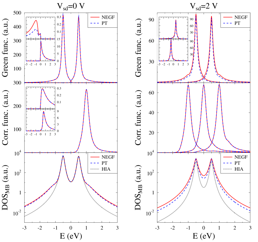
Figure 4: Non-degenerate, $\varepsilon_{a}\neq\varepsilon_{b}$, two-level system (HOMO-LUMO) junction. Exact NEGF results (solid line, red) are compared with diagrammatic perturbation theory (PT) simulations (dashed line, blue) for equilibrium ($V_{sd}=0$, left) and nonequilibrium ($V_{sd}=2$ V, right) junctions. Top graphs show Green functions $\mbox{Im}\,G^{<}_{11}(E)$, $-\mbox{Im}\,G^{>}_{44}(E)$ (main panel), $\mbox{Im}\,G^{<}_{33}(E)$ (top inset), and $-\mbox{Im}\,G^{>}_{11}(E)$ (bottom inset). Middle graphs show correlation functions $C^{>}_{31,13}(E)$ (rightmost peak in the main panel), $C^{>}_{13,31}(E)$ (top inset or leftmost peak in the main panel), and $C^{>}_{33,33}(E)$ (bottom inset or central peak in the main panel). Bottom graphs show many-body spectral function, $i\sum_{m}\left(G^{>}_{mm}(E)-G^{<}_{mm}(E)\right)$; dotted line (black) shows results of HIA calculations. See text for parameters.

IV Numerical results

Here we present simulations within the generic quantum dot model of Section III illustrating viability of the diagrammatic perturbation technique. We start from a non-interacting case, $U=0$, where exact solution is known from the usual NEGF. Simulations within the perturbation theory (PT) will be compared to the exact results.

Figure 4 shows results for a non-degenerate two-level system junction. Parameters of the simulations are $T=300$ K, $\varepsilon_{a}=-0.5$ eV, $\varepsilon_{b}=0.5$ eV, $U=0$, $\Gamma^{K}_{aa}=\Gamma^{K}_{bb}=0.1$ eV and $\Gamma^{K}_{ab}=\Gamma^{K}_{ba}=0$ ($K=L,R$). Fermi energy is taken as origin, $E_{F}=0$, and bias is applied symmetrically $\mu_{L/R}=E_{F}\pm V_{sd}/2$. Calculations are performed on a grid spanning region from $-6$ to $6$ eV with step $0.005$ eV. One sees that diagrammatic perturbation theory (dashed lines in Fig. 4) reproduces exact results (solid lines in Fig. 4) quite accurately. Taking into account that we build our consideration on top of the equilibrium theory Izyumov and Skryabin (1988); Ovchinnikov and Val’kov (2004), it is interesting to note that in some cases nonequilibrum results appear to be closer to exact data (compare top insets in the left and right top panels of Fig. 4). Another important observation comes from comparison of the PT and HIA results to exact data (compare dashed and dotted to solid lines in bottom panels of Fig. 4). In this calculation (with dominance of single electron tunneling) the main difference between the two approximations comes from second diagram in the middle panel of Fig. 3. This diagram was omitted in most previous Hubbard NEGF considerations.

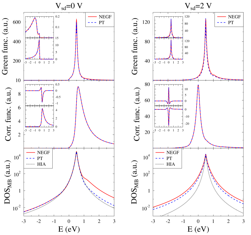
Figure 5: Degenerate, $\varepsilon_{a}=\varepsilon_{b}$, two-level system (HOMO-LUMO) junction. Exact NEGF results (solid line, red) are compared with diagrammatic perturbation theory (PT) simulations (dashed line, blue) for equilibrium ($V_{sd}=0$, left) and nonequilibrium ($V_{sd}=2$ V, right) junctions. Top graphs show Green functions $-\mbox{Im}\,G^{>}_{11}(E)$ (main panel), $\mbox{Im}\,G^{<}_{22}(E)$ (top inset), and $\mbox{Im}\,G^{<}_{11}(E)$ (bottom inset). Middle graphs show correlation functions $C^{>}_{33,33}(E)$ (main panel), $C^{>}_{13,13}(E)$ (top inset), and $C^{>}_{13,44}(E)$ (bottom inset). Bottom graphs show many-body spectral function, $i\sum_{m}\left(G^{>}_{mm}(E)-G^{<}_{mm}(E)\right)$; dotted line (black) shows results of HIA calculations. See text for parameters.

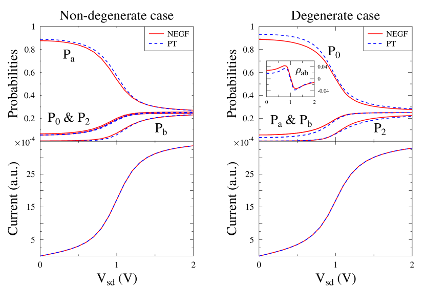
Figure 6: Non-interacting junction. Exact NEGF results (solid line, red) are compared with diagrammatic perturbation theory (PT) simulations (dashed line, blue). Shown are state probabilities (top panels) and current (bottom panels) vs. applied bias $V_{sd}$ for non-degenerate (left) and degenerate (right) cases of Figs. 4 and 5, respectively. Inset in the top right panel shows coherence vs. applied bias. See text for parameters.

Results for degenerate two-level system are presented in Fig. 5. Here $\varepsilon_{a}=\varepsilon_{b}=0.5$ eV and $\Gamma^{K}_{ab}=\Gamma^{K}_{ba}=0.05$ eV ($K=L,R$). Other parameters are as in Fig. 4. Also here PT theory demonstrates good approximation to the exact results and an advantage as compared to the HIA simulations.

Figure 6 shows currents and state probabilities as functions of applied bias for the two cases presented in Figs. 4-5. One sees that PT yields reasonable approximation to the exact results including the coherence (see inset in the right top panel) and perfect agreement for current-voltage characteristic.

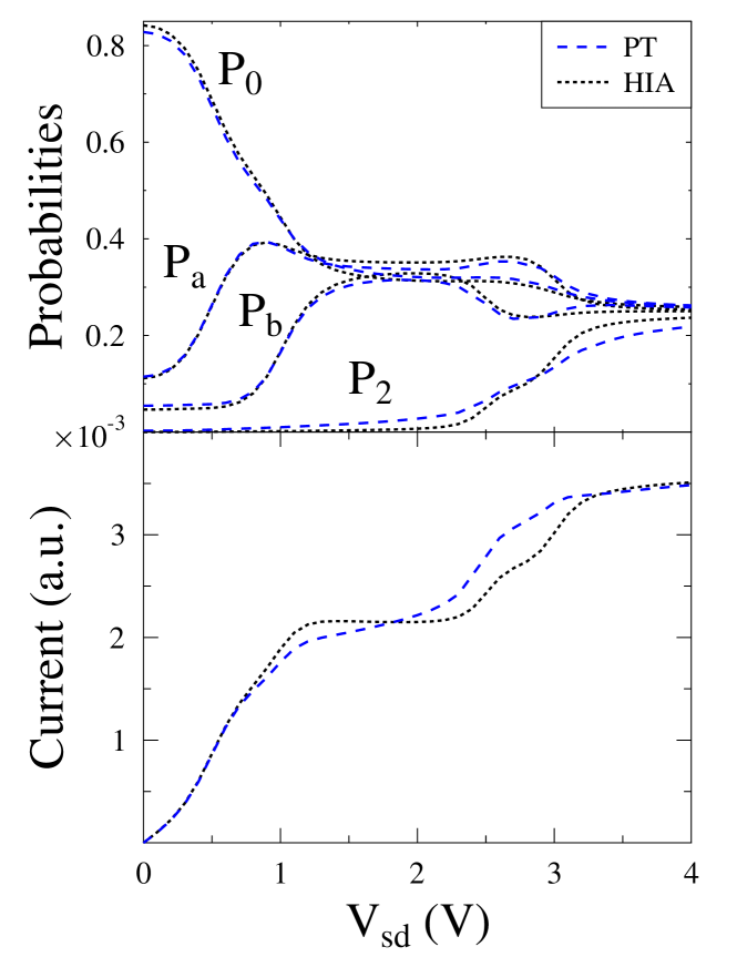
Figure 7: Quantum dot junction in the Coulomb blockade regime Diagrammatic perturbation theory (PT) simulations (dashed line, blue) are compared with the HIA (dotted line, black). Shown are state probabilities (top panel) and current (bottom panel) vs. applied bias $V_{sd}$. See text for parameters.

We now consider interacting junctions, $U\neq 0$. The Hubbard NEGF treatment (auxiliary fields formulation) of quantum-dot junction in the Coulomb blockade regime was discussed in details in Ref. Fransson (2005). Figure 7 shows that the second order PT (Fig. 3) yields similar results in this regime. Here parameters of the simulation are $\varepsilon_{a}=0.25$ eV, $\varepsilon_{b}=0.5$ eV, and $U=1$ eV. Other parameters are as in Fig. 4.

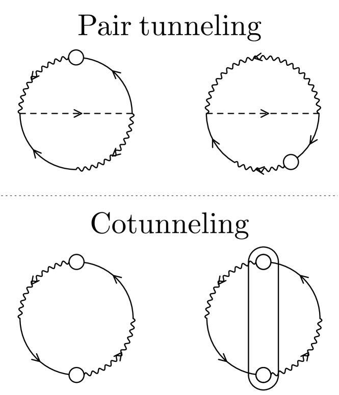
Figure 8: Diagrams responsible for pair (top) and cotunneling (bottom) transport in the negative-U model.

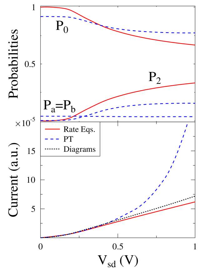
Figure 9: Pair electron tunneling in junction. Shown are state probabilities (top panel) and current (bottom panel) vs. applied bias $V_{sd}$. Diagrammatic perturbation theory (PT) simulations (dashed line, blue) are compared with the rate equation results of Ref. Koch et al. (2006) (solid line, red). Bottom panel also presents contribution to the current from diagrams of Fig. 8 (dotted line, black). See text for parameters.

Finally, we consider regime of pair electron tunneling in junctions. Within negative-U model this regime was examined in Ref. Koch et al. (2006) using the Schrieffer-Wolf transformation of the Hubbard Hamiltonian and evaluating Golden rule rates after the transformation. Noting that result of the Schrieffer-Wolf transformation can be effectively achieved within second order perturbation theory Martin and Mozyrsky (2005), and keeping in mind that in the Hubbard NEGF expression for current,

$$I_{K}(t)=2\,\mbox{Re}\,\int_{-\infty}^{t}dt^{\prime}\,$$ (21)

$$\qquad\mbox{Tr}\bigg{[}G^{>}(t,t^{\prime})\,\sigma_{K}^{<}(t^{\prime},t)-G^{<}(t,t^{\prime})\,\sigma_{K}^{>}(t^{\prime},t)\bigg{]}$$

(here $K=L,R$ and $\mbox{Tr}[\ldots]$ is trace over single-electron transitions (15)), two orders in coupling (8) enter via self-energy $\Sigma_{K}$, It is natural to expect that pair tunneling is given by second-order diagrams in Fig. 3 augmented by self-energy (wavy) line of Eq. (21). Indeed, one can show that results of Ref. Koch et al. (2006) can be obtained from (non-dressed) diagrams presented in Fig. 8 (see Appendix E for details). One sees that the pair tunneling results from second order diagrams involving two-electron propagator (first diagram in the middle panel and last diagram in the bottom panel of Fig. 3), while cotunneling results from the diagrams involving single-electron propagators (last diagram of the middle panel and first diagram of the bottom panel of Fig. 3). Note that for either pair or cotunneling only the sum of both self-energy and vertex diagrams is capable to provide correct results.

Figure 9 compares results of the PT simulation (dashed line) with rate equation results of Ref. Koch et al. (2006) (solid line). Calculations are performed for the negative-U model with parameters $\varepsilon_{a}=\varepsilon_{b}=2$ eV and $U=-3.8$ eV. Other parameters are as in Fig. 4. We note that contrary to previous results fourth order PT is required here. The PT takes broadening into account which leads to small non-zero values for the probabilities $P_{a}$ and $P_{b}$ of single-electron states (see top panel). Current-voltage characteristic (bottom panel) is almost identical to that of rate equations at low bias, $V_{sd}<0.5$ V, and deviates at higher biases, where contribution of the single-particle tunneling is non-negligible.

V Conclusion

We present a nonequilibrium flavor of diagrammatic technique for Hubbard Green functions. The technique is suitable for description of nonequilibrium steady-states in junctions. We assume that initial state of (uncoupled) system and baths does not impact nonequilibrium steady-state, which allows to utilize equilibrium considerations for the Hubbard lattice models for evaluation of zero-order (uncoupled) correlation functions of Hubbard operators. The latter leads to a nonequilibrium diagrammatic expansion for the Hubbard NEGF on the Keldysh contour. Similarly, one can consider diagrammatic expansion for multi-time correlation functions on the contour.

We illustrate viability of the approach with numerical examples of transport in non-interacting (two-level system) and interacting (quantum dot) junctions. For non-interacting system we compare the diagrammatic PT to exact NEGF results, and show that the approach is quite accurate (for both non-degenerate and degenerate cases) already at second order of the PT. Interacting calculations are compared with similar considerations available in the literature. In particular, quantum dot junction results are compared to the auxiliary-field approach to the Hubbard NEGF. Results of the PT simulations within the negative-U model for pair electron tunneling are compared with rate equations applied to Schrieffer-Wolf transformed Hamiltonian. We show importance of the correlation (vertex) diagrams, which were omitted in previous Hubbard NEGF considerations.

The diagrammatic PT for Hubbard NEGF contributes to development of tools for the nonequilibrium atomic limit, where the response of a molecular junction to external perturbations is characterized utilizing many-body states of the isolated molecule while coupling to the contacts is treated perturbatively. Such an approach yields a possibility of incorporating standard quantum chemistry and nonlinear optical spectroscopy methods (mostly formulated for isolated molecules and utilizing many-body states) to description of quickly developing field of nanoscale optoelectronics of molecular junctions. It may also be useful in thermodynamic studies of thermoelectric and photovoltaic molecular devices. Finally we note that while approaches utilizing many-body states description were successfully implemented in a number ab initio simulations Hettler et al. (2003); Yeganeh et al. (2009); Zyazin et al. (2010); Misiorny et al. (2013); White et al. (2014b), combination of such formulations with quasiparticle based approaches capitalizing on ability of the former to treat strong local interactions and scalability of the latter would be advantageous. This is a goal of our future research.

Appendix A Commutation relations

Here we present commutation relations between Hubbard operators utilized in derivation of diagrams. Note that the commutation relations can be formulated in a compact form utilizing a notion of root vectors Ovchinnikov and Val’kov (2004). However it is hard to keep track of the physics represented by the diagrams constructed utilizing the notion. Thus here we present explicit commutation relations of operators relevant for the quantum dot model

$$\begin{split}&\{\hat{X}_{m};\hat{X}_{m^{\prime}}\}=\delta_{m,\bar{m}^{\prime}}\hat{X}_{02}\\ &[\hat{X}_{m};\hat{X}_{02}^{\dagger}]=(-1)^{m}\hat{X}_{\bar{m}}^{\dagger}\\ &[\hat{X}_{m};\hat{N}]=-\hat{X}_{m}\\ &[\hat{X}_{m};\hat{F}_{m_{1}m_{2}}]=\eta(m,m_{1}m_{2})\hat{X}_{\gamma(m,m_{1}m_{2})}\\ &[\hat{X}_{02};\hat{X}_{m}^{\dagger}]=(-1)^{m}\hat{X}_{\bar{m}}\\ &[\hat{X}_{02};\hat{F}_{m_{1}m_{2}}]=\delta_{m_{1},m_{2}}(-1)^{m_{1}}\hat{X}_{02}\\ &[\hat{X}_{02};\hat{N}]=-2\,\hat{X}_{02}\end{split}$$ (22)

with other commutators zero. Here $\bar{m}=3-m$,

$$\hat{F}_{mm^{\prime}}\equiv\{\hat{X}_{m};\hat{X}_{m^{\prime}}^{\dagger}\}\qquad\hat{N}\equiv[\hat{X}_{02};\hat{X}_{02}^{\dagger}]$$ (23)

$$\eta(m,m_{1}m_{2})=\delta_{m_{1},m_{2}}(-1)^{m_{1}}-\delta_{m_{1},m_{2}\pm 2}(-1)^{m}$$ (24)

$$\gamma(m,m_{1}m_{2})=\delta_{m_{1},m_{2}}m+\delta_{m_{1},m_{2}\pm 2}(m\pm 2)$$ (25)

Appendix B Fourth order expressions for Green function (2) self-energy and vertex

Dressed fourth order contributions to self-energy and vertex of Green function (2) are

$$\Sigma_{mm^{\prime}}^{(4)}(\tau,\tau^{\prime})=-\sum_{\{m\}}\int_{c}d\tau_{1}\int_{c}d\tau_{2}\,$$ (26)

$$\bigg{(}\eta(m_{5},mm_{1})\,\eta(m_{6},m_{3}m_{4})\delta_{\gamma(m_{6},m_{3}m_{4}),m^{\prime}}\sigma_{m_{1}m_{2}}(\tau,\tau_{2})\,g_{m_{2}m_{3}}(\tau_{2},\tau^{\prime})\,\sigma_{m_{4}m_{7}}(\tau,\tau_{1})\,g_{m_{7}m_{5}}(\tau_{1},\tau)\,g_{\gamma(m_{5},mm_{1})m_{6}}(\tau,\tau^{\prime})$$

$$+(-1)^{m}d_{02}(\tau,\tau^{\prime})\,\sigma_{\bar{m}^{\prime}m_{2}}(\tau^{\prime},\tau_{2})\bigg{[}(-1)^{m^{\prime}}d_{02}(\tau_{2},\tau)\,\sigma_{mm_{1}}(\tau,\tau_{1})\,g_{m_{1}\bar{m}_{2}}(\tau_{1},\tau_{2})+i\,g_{m_{2}m_{1}}(\tau_{2},\tau_{1})\,F_{m_{1}m_{3}}(\tau_{1})\,\sigma_{m_{3}\bar{m}}(\tau_{1},\tau)\bigg{]}\bigg{)}$$

$$\Delta^{(4)}_{mm^{\prime}}(\tau,\tau^{\prime})=-\sum_{\{m\}}\int_{c}d\tau_{1}\int_{c}d\tau_{2}\int_{c}d\tau_{3}$$ (27)

$$\bigg{(}(-1)^{m^{\prime}}\eta(m_{4},mm_{5})\,\sigma_{m_{5}m_{3}}(\tau,\tau_{3})\,g_{m_{3}\bar{m}_{2}}(\tau_{3},\tau_{2})\,g_{\gamma(m_{4},mm_{5})m_{1}}(\tau,\tau_{1})\,F_{m_{1}m_{6}}(\tau_{1})\,\sigma_{m_{6}m_{2}}(\tau_{1},\tau_{2})\,d_{02}(\tau_{2},\tau^{\prime})\,g_{\bar{m}^{\prime}m_{4}}(\tau^{\prime},\tau)$$

$$+(-1)^{m+m^{\prime}}d_{02}(\tau,\tau^{\prime})\,g_{\bar{m}^{\prime}m_{1}}(\tau^{\prime},\tau_{1})\,F_{m_{1}m_{4}}(\tau_{1})\,\sigma_{m_{4}m_{2}}(\tau_{1},\tau_{2})\,d_{02}(\tau_{2},\tau)\,\sigma_{mm_{3}}(\tau,\tau_{3})\,g_{m_{3}\bar{m}_{2}}(\tau_{3},\tau_{2})$$

$$+i\,\eta(m_{7},m_{6},m^{\prime})\,C_{mm_{5},m_{1}m_{4}}(\tau,\tau_{1})\,\sigma_{m_{5}m_{3}}(\tau,\tau_{3})\,g_{m_{3}m_{6}}(\tau_{3},\tau^{\prime})\,g_{\gamma(m_{7},m_{6}m^{\prime})\,m_{1}}(\tau^{\prime},\tau_{1})\,\sigma_{m_{4}m_{2}}(\tau_{1},\tau_{2})\,g_{m_{2}m_{7}}(\tau_{2},\tau^{\prime})$$

$$-i\,(-1)^{m^{\prime}}C_{mm_{5},m_{1}m_{4}}(\tau,\tau_{1})\,\sigma_{m_{5}m_{3}}(\tau,\tau_{3})\,g_{m_{3}\bar{m}_{2}}(\tau_{3},\tau_{2})\,\sigma_{m_{4}m_{2}}(\tau_{1},\tau_{2})\,d_{02}(\tau_{2},\tau^{\prime})\,g_{\bar{m}^{\prime}m_{1}}(\tau^{\prime},\tau_{1})$$

$$+i\,\eta(m_{7},mm_{5})\,C_{m_{1}m_{4},m_{6}m^{\prime}}(\tau_{1},\tau^{\prime})\,\sigma_{m_{5}m_{3}}(\tau,\tau_{3})\,g_{m_{3}m_{6}}(\tau_{3},\tau^{\prime})\,g_{\gamma(m_{7},mm_{5})\,m_{1}}(\tau,\tau_{1})\,\sigma_{m_{4}m_{2}}(\tau_{1}\tau_{2})\,g_{m_{2}m_{7}}(\tau_{2},\tau)$$

$$-i\,\eta(m_{6},mm_{5})\,C_{m_{1}m_{4},m_{6}m^{\prime}}(\tau_{1},\tau^{\prime})\,\sigma_{m_{5}m_{3}}(\tau,\tau_{3})\,g_{m_{3},m_{1}}(\tau_{3},\tau_{1})\,\sigma_{m_{4}m_{2}}(\tau_{1},\tau_{2})\,g_{m_{2}m_{7}}(\tau_{2},\tau)\,g_{\gamma(m_{6},mm_{5})\,m_{8}}(\tau,\tau^{\prime})$$

$$-i(-1)^{m_{1}}C_{m_{4}m_{3}.m_{6}m^{\prime}}(\tau_{3},\tau^{\prime})\,\sigma_{m_{3}\bar{m}}(\tau_{3},\tau)\,d_{02}(\tau,\tau_{1})\,g_{\bar{m}_{1}m_{6}}(\tau_{1},\tau^{\prime})\,\sigma_{m_{1}m_{2}}(\tau_{1},\tau_{2})\,g_{m_{2}m_{4}}(\tau_{2},\tau_{3})$$

$$+i(-1)^{m_{1}}C_{m_{4}m_{3},m_{6}m^{\prime}}(\tau_{3},\tau^{\prime})\,\sigma_{m_{3}\bar{m}}(\tau_{3},\tau)\,d_{02}(\tau,\tau_{1})\,\sigma_{m-1m_{2}}(\tau_{1},\tau_{2})\,g_{m_{2}m_{6}}(\tau_{2},\tau^{\prime})\,g_{\bar{m}_{1}m_{4}}(\tau_{1},\tau_{3})\bigg{)}$$

Appendix C Diagrammatic expansion for Green function (19)

Diagrammatic expansion for the two-particle Green function follows the same rules as for the single-particle Green function. Second order diagrams for the self-energy $\Sigma_{02}$ and vertex $\Delta_{02}$ are shown in Fig. 10. Explicit dressed expressions are

$$\Sigma^{(2)}_{02}(\tau,\tau^{\prime})= i\sum_{m_{1},m_{2}}(-1)^{m_{1}}\sigma_{m_{1}m_{2}}(\tau,\tau^{\prime})\,g_{\bar{m}_{1}\bar{m}_{2}}(\tau,\tau^{\prime})$$ (28)

$$\Delta^{(2)}_{02}(\tau,\tau^{\prime})= -i\sum_{\begin{subarray}{c}m_{1},m_{2}\\ m_{3},m_{4}\end{subarray}}(-1)^{m_{1}+m_{3}}g_{\bar{m}_{1}m_{3}}(\tau,\tau^{\prime})$$ (29)

$$\times \int_{c}d\tau_{1}\,\sigma_{m_{1}m_{2}}(\tau,\tau_{1})\,g_{m_{2}m_{4}}(\tau_{1},\tau^{\prime})\,F_{m_{4}\bar{m}_{3}}(\tau^{\prime})$$

Figure 10: Second order (non-dressed) contributions to self-energy $\Sigma_{02}$ (left) and vertex $\Delta_{02}$ (right).

Dressed fourth order contributions are

$$S_{02}^{(4)}(\tau,\tau^{\prime})=\sum_{\{m\}}(-1)^{m}\int_{c}d\tau_{1}\int_{c}d\tau_{2}\,$$ (30)

$$\bigg{(}g_{m_{1}m_{2}}(\tau_{1},\tau_{2})\,g_{\bar{m},\bar{m}^{\prime}}(\tau,\tau^{\prime})-g_{m_{1}\bar{m}^{\prime}}(\tau_{1},\tau^{\prime})\,g_{\bar{m}m_{2}}(\tau,\tau_{2})\bigg{)}$$

$$\times\sigma_{mm_{1}}(\tau,\tau_{1})\,F_{m_{2}m_{3}}(\tau_{2})\,\sigma_{m_{3}m^{\prime}}(\tau_{2},\tau^{\prime})$$

$$\Delta_{02}^{(4)}(\tau,\tau^{\prime})=i\sum_{\{m\}}(-1)^{m}\int_{c}d\tau_{1}\int_{c}d\tau_{2}\int_{c}d\tau_{3}\,$$ (31)

$$\bigg{(}g_{m_{1}m_{2}}(\tau_{1},\tau_{2})\,g_{\bar{m}\bar{m}_{4}}(\tau,\tau_{3})-g_{m_{1}\bar{m}_{4}}(\tau_{1},\tau_{4})\,g_{\bar{m}m_{2}}(\tau,\tau_{2})\,\bigg{)}$$

$$\times\sigma_{mm_{1}}(\tau,\tau_{1})\,\sigma_{m_{3}m_{4}}(\tau_{2},\tau_{3})\,d_{02}(\tau_{3},\tau^{\prime})\,C_{02\,02,m_{2}m_{3}}(\tau^{\prime},\tau_{2})$$

Note that

$$C_{02\,02,m_{2}m_{3}}(\tau,\tau^{\prime})\equiv C_{0S\,0S,m_{2}m_{3}}(\tau,\tau^{\prime})-C_{S2\,S2,m_{2}m_{3}}(\tau,\tau^{\prime})$$ (32)

with $S=a$ or $b$.

Appendix D Diagrammatic expansion for correlation function (20)

Diagrammatic expansion for correlation functions follows contraction rules formulated in Section II. Resummation of the diagrams was discussed in Ref. Izyumov et al. (1994).

In actual calculations we only utilized a single bubble diagram. Its explicit expression is

$$C_{m_{1}m_{2},m_{3}m_{4}}(\tau,\tau^{\prime})=\sum_{m_{5},m_{6}}\eta(m_{5},m_{1}m_{2})\,\eta(m_{6},m_{3}m_{4})$$ (33)

$$\qquad\qquad g_{\gamma(m_{5},m_{1}m_{2})\,m_{6}}(\tau,\tau^{\prime})\,g_{\gamma(m_{6},m_{3}m_{4})\,m_{5}}(\tau^{\prime},\tau)$$

Numerical results presented in Section IV show that the approximation appears to be quite accurate.

Appendix E Pair and cotunneling diagrams

Here we prove that diagrams of Fig. 8 represent pair and cotunneling.

Second order contribution in molecule-contacts coupling, Eq. (8), to the Hubbard Green function, Eq. (2), is

$$G_{mm^{\prime}}^{(2)}(\tau,\tau^{\prime})=\sum_{\begin{subarray}{c}m_{1},k_{1},\sigma_{1}\\ m_{2},k_{2},\sigma_{2}\end{subarray}}\int_{c}d\tau_{1}\int_{c}d\tau_{2}\,V_{k_{1}\sigma_{1},m_{1}}\,V_{m_{2},k_{2}\sigma_{2}}$$ (34)

$$\langle T_{c}\,\hat{X}_{m}(\tau)\,\hat{X}_{m^{\prime}}^{\dagger}(\tau^{\prime})\,\hat{c}_{k_{1}\sigma_{1}}^{\dagger}(\tau_{1})\,\hat{X}_{m_{1}}(\tau_{1})\,\hat{X}_{m_{2}}^{\dagger}(\tau_{2})\,\hat{c}_{k_{2}\sigma_{2}}(\tau_{2})\rangle_{0}$$

We now can apply contraction rules of Section II, which leads to a set of diagrams presented in Fig. 3. These augmented with the self-energy $\sigma_{K}$ lines results in a set of contributions to the current (21). We then project these contributions using connection between scattering theory and the Keldysh contour formulation (as discussed in Ref. Galperin et al. (2015)) and employing the Langreth (contour deformation) rules Haug and Jauho (2008). In particular, below we show that for diagrams in Fig. 8 one can identify projections of contour variables $\tau_{1,2}$ onto real time axis $t_{1,2}$ which after substituting lesser and greater projections of (34) into (21) yield pair tunneling and cotunneling.

Figure 11: Langreth projections of contour variables $\tau_{1,2}$ in Eq. (34) which yield pair tunneling contribution to the current, Eq. (21). Left (right) panel shows projections for the in-scattering (out-scattering) flux.

For pair tunneling we use top diagrams of Fig. 8 and projections shown in Fig. 11 in Eq. (21). The projections lead to integrals

$$\int_{-\infty}^{+\infty}d(t^{\prime}-t)\ldots\int_{-\infty}^{0}d(t_{1}-t)\ldots\int_{-\infty}^{0}d(t_{2}-t^{\prime})\ldots$$ (35)

We then perform the integrations for the top diagrams of Fig. 8 employing the following expressions for lesser and greater projections of zero-order propagators

$$g_{m}^{(0)\,>}(t,t^{\prime})= -i\frac{P_{m(1)}}{P_{m(1)}+P_{m(2)}}e^{-iE_{m}(t-t^{\prime})}$$ (36)

$$g_{m}^{(0)\,<}(t,t^{\prime})= +i\frac{P_{m(2)}}{P_{m(1)}+P_{m(2)}}e^{-iE_{m}(t-t^{\prime})}$$ (37)

$$d_{02}^{(0)\,>}(t,t^{\prime})= -i\frac{P_{0}}{P_{0}-P_{2}}e^{-iE_{02}(t-t^{\prime})}$$ (38)

$$d_{02}^{(0)\,<}(t,t^{\prime})= -i\frac{P_{2}}{P_{0}-P_{2}}e^{-iE_{02}(t-t^{\prime})}$$ (39)

Here $P_{S}$ ($S=0,a,b,2$) is the probability to find the system in state $\lvert S\rangle$, $P_{m(1)}$ and $P_{m(2)}$ are probabilities for the first and second state of the transitions defined in Eq. (15), $E_{m}\equiv E_{m(2)}-E_{m(1)}$, and $E_{02}\equiv E_{2}-E_{0}$. Taking into account that for $\varepsilon_{a,b}\gg 0$ and $|U|\gg 1$ only $P_{0}$ and $P_{2}$ are non-zero we get the following contribution to the current (21)

$$I_{K}=W^{K}_{2\leftarrow 0}\,P_{0}-W^{K}_{0\leftarrow 2}\,P_{2}$$ (40)

with the rates

$$W^{K}_{2\leftarrow 0}=\int\frac{dE}{2\pi}\,\bigg{\lvert}\frac{1}{E-\varepsilon+i\delta}-\frac{1}{E-\varepsilon-U+i\delta}\bigg{\rvert}^{2}$$ (41)

$$\quad\times\Gamma^{K}f_{K}(E_{02}-E)\sum_{K^{\prime}=L,R}\Gamma^{K^{\prime}}f_{K^{\prime}}(E)$$

$$W^{K}_{0\leftarrow 2}=\int\frac{dE}{2\pi}\,\bigg{\lvert}\frac{1}{E-\varepsilon+i\delta}-\frac{1}{E-\varepsilon-U+i\delta}\bigg{\rvert}^{2}$$ (42)

$$\quad\times\Gamma^{K}[1-f_{K}(E_{02}-E)]\sum_{K^{\prime}=L,R}\Gamma^{K^{\prime}}[1-f_{K^{\prime}}(E)]$$

Here $\varepsilon_{a}=\varepsilon_{b}\equiv\varepsilon$, $\Gamma^{K}_{aa}=\Gamma^{K}_{bb}\equiv\Gamma^{K}$, $\Gamma\equiv\Gamma^{L}+\Gamma^{R}$, $\Gamma^{K}_{ab}=\Gamma^{K}_{ba}=0$, $f_{K}(E)$ is the Fermi-Dirac thermal distribution in contact $K$, and $\delta\to 0+$. These are exactly the pair tunneling rates originally derived in Ref. Koch et al. (2006).

Similarly, employing bottom diagrams of Fig. 8 and projections presented in Fig. 12, and utilizing Eqs. (36)-(39) and zero-order expression for correlation functions

$$C^{(0)}_{mm,m^{\prime}m^{\prime}}(\tau,\tau^{\prime})=\delta_{m,m^{\prime}}F^{(0)}_{mm}-F_{mm}^{(0)}\,F_{m^{\prime}m^{\prime}}^{(0)}$$ (43)

$$F_{mm}^{(0)}=P_{m(1)}+P_{m(2)}$$ (44)

we can derive expressions for cotunneling rates in a similar fashion.

Figure 12: Langreth projections of contour variables $\tau_{1,2}$ in Eq. (34) which yield cotunneling contribution to the current, Eq. (21). Left (right) panel shows projections for the in-scattering (out-scattering) flux.

References

- Aviram and Ratner (1974) A. Aviram and M. A. Ratner, Chem. Phys. Lett. 29, 277 (1974).
- Reed et al. (1997) M. A. Reed, C. Zhou, C. J. Muller, T. P. Burgin, and J. M. Tour, Science 278, 252 (1997).
- Ratner (2013) M. Ratner, Nat Nano 8, 378 (2013).
- van der Molen et al. (2013) S. J. van der Molen, R. Naaman, E. Scheer, J. B. Neaton, A. Nitzan, D. Natelson, N. J. Tao, H. S. J. van der Zant, M. Mayor, M. Ruben, M. Reed, and M. Calame, Nature Nanotech. 8, 385 (2013).
- Aradhya and Venkataraman (2013) S. V. Aradhya and L. Venkataraman, Nat Nano 8, 399 (2013).
- Kadanoff and Baym (1962) L. P. Kadanoff and G. Baym, Quantum Statistical Mechanics, edited by D. Pines (W. A. Benjamin, Inc., New York, 1962).
- Keldysh (1965) L. V. Keldysh, Sov. Phys. JETP 20, 1018 (1965).
- Danielewicz (1984) P. Danielewicz, Ann. Phys. 152, 239 (1984).
- Rammer and Smith (1986) J. Rammer and H. Smith, Rev. Mod. Phys. 58, 323 (1986).
- Parr and Yang (1989) R. G. Parr and W. Yang, Density-Functional Theory of Atoms and Molecules (Oxford University Press, 1989).
- Dreizler and Gross (1990) R. M. Dreizler and E. K. U. Gross, Density-Functional Theory of Atoms and Molecules (Springer-Verlag, 1990).
- Damle et al. (2002) P. Damle, A. W. Ghosh, and S. Datta, Chemical Physics 281, 171 (2002).
- Xue et al. (2002) Y. Xue, S. Datta, and M. A. Ratner, Chemical Physics 281, 151 (2002).
- Brandbyge et al. (2002) M. Brandbyge, J.-L. Mozos, P. Ordejón, J. Taylor, and K. Stokbro, Phys. Rev. B 65, 165401 (2002).
- Sergueev et al. (2005) N. Sergueev, D. Roubtsov, and H. Guo, Phys. Rev. Lett. 95, 146803 (2005).
- Frederiksen et al. (2007) T. Frederiksen, M. Paulsson, M. Brandbyge, and A.-P. Jauho, Phys. Rev. B 75, 205413 (2007).
- Schmaus et al. (2011) S. Schmaus, A. Bagrets, Y. Nahas, T. K. Yamada, A. Bork, M. Bowen, E. Beaurepaire, F. Evers, and W. Wulfhekel, Nat Nano 6, 185 (2011).
- Avriller and Frederiksen (2012) R. Avriller and T. Frederiksen, Phys. Rev. B 86, 155411 (2012).
- Chen et al. (1999) J. Chen, M. A. Reed, A. M. Rawlett, and J. M. Tour, Science 286, 1550 (1999).
- Rinkiö et al. (2010) M. Rinkiö, A. Johansson, V. Kotimäki, and P. T—”ormä, ACS Nano 4, 3356 (2010).
- Blum et al. (2005) A. S. Blum, J. G. Kushmerick, D. P. Long, C. H. Patterson, J. C. Yang, J. C. Henderson, Y. Yao, J. M. Tour, R. Shashidhar, and B. R. Ratna, Nature Materials 4, 167 (2005).
- Kiehl et al. (2006) R. A. Kiehl, J. D. Le, P. Candra, R. C. Hoye, and T. R. Hoye, Appl. Phys. Lett. 88, 172102 (2006).
- Lörtscher et al. (2006) E. Lörtscher, J. W. Ciszek, J. Tour, and H. Riel, Small 2, 973 (2006).
- Wei et al. (2007) J. H. Wei, S. J. Xie, L. M. Mei, J. Berakdar, and Y. Yan, Organic Electronics 8, 487 (2007).
- Wu et al. (2008) S. W. Wu, N. Ogawa, G. V. Nazin, and W. Ho, J. Phys. Chem. C 112, 5241 (2008).
- Ho (2002) W. Ho, The Journal of Chemical Physics 117, 11033 (2002).
- Seideman (2003) T. Seideman, Journal of Physics: Condensed Matter 15, R521 (2003).
- van der Molen and Liljeroth (2010) S. J. van der Molen and P. Liljeroth, Journal of Physics: Condensed Matter 22, 133001 (2010).
- Osorio et al. (2010) E. A. Osorio, M. Ruben, J. S. Seldenthuis, J. M. Lehn, and H. S. J. van der Zant, Small 6, 174 (2010).
- Komeda et al. (2011) T. Komeda, H. Isshiki, J. Liu, Y.-F. Zhang, N. Lorente, K. Katoh, B. K. Breedlove, and M. Yamashita, Nat Commun 2, 217 (2011).
- Schirm et al. (2013) C. Schirm, M. Matt, F. Pauly, J. C. Cuevas, P. Nielaba, and E. Scheer, Nat Nano 8, 645 (2013).
- Baer and Neuhauser (2005) R. Baer and D. Neuhauser, Phys. Rev. Lett. 94, 043002 (2005).
- Livshits and Baer (2007) E. Livshits and R. Baer, Phys. Chem. Chem. Phys. 9, 2932 (2007).
- Refaely-Abramson et al. (2012) S. Refaely-Abramson, S. Sharifzadeh, N. Govind, J. Autschbach, J. B. Neaton, R. Baer, and L. Kronik, Phys. Rev. Lett. 109, 226405 (2012).
- Liu et al. (2014) Z.-F. Liu, S. Wei, H. Yoon, O. Adak, I. Ponce, Y. Jiang, W.-D. Jang, L. M. Campos, L. Venkataraman, and J. B. Neaton, Nano Letters 14, 5365 (2014).
- Baratz et al. (2013) A. Baratz, M. Galperin, and R. Baer, J. Phys. Chem. C 117, 10257 (2013).
- Baratz et al. (2014) A. Baratz, A. J. White, M. Galperin, and R. Baer, J. Phys. Chem. Lett. 5, 3545 (2014).
- Gaudoin and Burke (2004) R. Gaudoin and K. Burke, Phys. Rev. Lett. 93, 173001 (2004).
- Baer (2008) R. Baer, J. Chem. Phys. 128, 044103 (2008).
- Bâldea (2016) I. Bâldea, Beilstein Journal of Nanotechnology 7, 418 (2016).
- Park et al. (2000) H. Park, J. Park, A. K. L. Lim, E. H. Anderson, A. P. Alivisatos, and P. L. McEuen, Nature 407, 57 (2000).
- Wurtz et al. (2007) G. A. Wurtz, P. R. Evans, W. Hendren, R. Atkinson, W. Dickson, R. J. Pollard, A. V. Zayats, W. Harrison, and C. Bower, Nano Letters 7, 1297 (2007).
- Repp et al. (2010) J. Repp, P. Liljeroth, and G. Meyer, Nature Physics 6, 975 (2010).
- Natelson et al. (2013) D. Natelson, Y. Li, and J. B. Herzog, Phys. Chem. Chem. Phys. 15, 5262 (2013).
- Schulz et al. (2015) F. Schulz, M. Ijas, R. Drost, S. K. Hamalainen, A. Harju, A. P. Seitsonen, and P. Liljeroth, Nat Phys 11, 229 (2015).
- Wagner et al. (2015) C. Wagner, M. F. B. Green, P. Leinen, T. Deilmann, P. Krüger, M. Rohlfing, R. Temirov, and F. S. Tautz, Phys. Rev. Lett. 115, 026101 (2015).
- Yeganeh et al. (2009) S. Yeganeh, M. A. Ratner, M. Galperin, and A. Nitzan, Nano Lett. 9, 1770 (2009).
- Gao and Galperin (2016a) Y. Gao and M. Galperin, The Journal of Chemical Physics 144, 244106 (2016a).
- White et al. (2014a) A. J. White, M. A. Ochoa, and M. Galperin, J. Phys. Chem. C 118, 11159 (2014a).
- Bâldea et al. (2010) I. Bâldea, H. Köppel, R. Maul, and W. Wenzel, J. Chem. Phys. 133, 014108 (2010).
- Wingreen and Meir (1994) N. S. Wingreen and Y. Meir, Phys. Rev. B 49, 11040 (1994).
- Aoki et al. (2014) H. Aoki, N. Tsuji, M. Eckstein, M. Kollar, T. Oka, and P. Werner, Rev. Mod. Phys. 86, 779 (2014).
- Eckstein and Werner (2010) M. Eckstein and P. Werner, Phys. Rev. B 82, 115115 (2010).
- Oh et al. (2011) J. H. Oh, D. Ahn, and V. Bubanja, Phys. Rev. B 83, 205302 (2011).
- White and Galperin (2012) A. J. White and M. Galperin, Phys. Chem. Chem. Phys. 14, 13809 (2012).
- White et al. (2012) A. J. White, B. D. Fainberg, and M. Galperin, J. Phys. Chem. Lett. 3, 2738 (2012).
- White et al. (2013) A. J. White, U. Peskin, and M. Galperin, Phys. Rev. B 88, 205424 (2013).
- White et al. (2014b) A. J. White, S. Tretiak, and M. Galperin, Nano Lett. 14, 699 (2014b).
- Chen et al. (2016) H.-T. Chen, G. Cohen, A. J. Millis, and D. R. Reichman, Phys. Rev. B 93, 174309 (2016).
- Galperin et al. (2008) M. Galperin, A. Nitzan, and M. A. Ratner, Phys. Rev. B 78, 125320 (2008).
- Fransson (2010) J. Fransson, Non-Equilibrium Nano-Physics - A Many-Body Approach (Springer-Verlag, 2010).
- Fransson et al. (2002) J. Fransson, O. Eriksson, and I. Sandalov, Phys. Rev. B 66, 195319 (2002).
- Fransson et al. (2004) J. Fransson, O. Eriksson, and I. Sandalov, Photonics and Nanostructures - Fundamentals and Applications 2, 11 (2004).
- Fransson (2005) J. Fransson, Phys. Rev. B 72, 075314 (2005).
- Sandalov and Nazmitdinov (2006) I. Sandalov and R. G. Nazmitdinov, J. Phys.: Condens. Matter 18, L55 (2006).
- Sandalov and Nazmitdinov (2007) I. Sandalov and R. G. Nazmitdinov, Phys. Rev. B 75, 075315 (2007).
- Mukamel (1995) S. Mukamel, Principles of Nonlinear Optical Spectroscopy, Oxford Series in Optical and Imaging Sciences, Vol. 6 (Oxford University Press, 1995).
- Gao and Galperin (2016b) Y. Gao and M. Galperin, J. Chem. Phys. 144, 174113 (2016b).
- Esposito et al. (2009) M. Esposito, U. Harbola, and S. Mukamel, Rev. Mod. Phys. 81, 1665 (2009).
- Izyumov and Skryabin (1988) Y. A. Izyumov and Y. N. Skryabin, Statistical Mechanics of Magentically Ordered Systems (Consultants Bureau, New York and London, 1988).
- Ovchinnikov and Val’kov (2004) S. G. Ovchinnikov and V. V. Val’kov, Systems Operators in the Theory of Strongly Correlated Electrons (Imperial College Press, 2004).
- Schoeller and Schön (1994) H. Schoeller and G. Schön, Phys. Rev. B 50, 18436 (1994).
- König et al. (1996) J. König, J. Schmid, H. Schoeller, and G. Schön, Phys. Rev. B 54, 16820 (1996).
- Schoeller (2000) H. Schoeller, Lecture Notes in Physics 544, 137 (2000).
- Leijnse and Wegewijs (2008) M. Leijnse and M. R. Wegewijs, Phys. Rev. B 78, 235424 (2008).
- Jin et al. (2008) J. Jin, X. Zheng, and Y. Yan, J. Chem. Phys. 128, 234703 (2008).
- Härtle et al. (2013) R. Härtle, G. Cohen, D. R. Reichman, and A. J. Millis, Phys. Rev. B 88, 235426 (2013).
- Yan (2014) Y. Yan, J. Chem. Phys. 140, 054105 (2014).
- Ye et al. (2016) L. Ye, X. Wang, D. Hou, R.-X. Xu, X. Zheng, and Y. Yan, Wiley Interdisciplinary Reviews: Computational Molecular Science , n/a (2016).
- Yan et al. (2016) Y. Yan, J. Jin, R.-X. Xu, and X. Zheng, Frontiers of Physics 11, 1 (2016).
- Fetter and Walecka (1971) A. L. Fetter and J. D. Walecka, Quantum Theory of Many-Particle Systems (McGraw-Hill Book Company, 1971).
- Haug and Jauho (2008) H. Haug and A.-P. Jauho, Quantum Kinetics in Transport and Optics of Semiconductors (Springer, Berlin Heidelberg, 2008).
- Galperin et al. (2007) M. Galperin, A. Nitzan, and M. A. Ratner, Phys. Rev. B 76, 035301 (2007).
- Pedersen et al. (2009) J. N. Pedersen, D. Bohr, A. Wacker, T. Novotný, P. Schmitteckert, and K. Flensberg, Phys. Rev. B 79, 125403 (2009).
- Koch et al. (2006) J. Koch, M. E. Raikh, and F. von Oppen, Phys. Rev. Lett. 96, 056803 (2006).
- Martin and Mozyrsky (2005) I. Martin and D. Mozyrsky, Phys. Rev. B 71, 165115 (2005).
- Hettler et al. (2003) M. H. Hettler, W. Wenzel, M. R. Wegewijs, and H. Schoeller, Phys. Rev. Lett. 90, 076805 (2003).
- Zyazin et al. (2010) A. S. Zyazin, J. W. G. van den Berg, E. A. Osorio, H. S. J. van der Zant, N. P. Konstantinidis, M. Leijnse, M. R. Wegewijs, F. May, W. Hofstetter, C. Danieli, and A. Cornia, Nano Lett. 10, 3307 (2010).
- Misiorny et al. (2013) M. Misiorny, M. Hell, and M. R. Wegewijs, Nat Phys 9, 801 (2013).
- Izyumov et al. (1994) Y. A. Izyumov, M. I. Katsnelson, and Y. N. Skryabin, Itinerant Electron Magnetism (in Russian) (Nauka, Moscow, 1994).
- Galperin et al. (2015) M. Galperin, M. A. Ratner, and A. Nitzan, J. Chem. Phys. 142, 137101 (2015).