The locally adapted parametric finite element method for interface problems on triangular meshes

Abstract

We present a locally adapted parametric finite element method for interface problems. For this adapted finite element method we show optimal convergence for elliptic interface problems with a discontinuous diffusion parameter. The method is based on the adaption of macro elements where a local basis represents the interface. The macro elements are independent of the interface and can be cut by the interface. A macro element which is a triangle in the triangulation is divided into four subtriangles. On these subtriangles, the basis functions of the macro element are interpreted as linear functions. The position of the vertices of these subtriangles is determined by the location of the interface in the case a macro element is cut by the interface. Quadrature is performed on the subtriangles via transformations to a reference element. Due to the locality of the method, its use is well suited on distributed architectures.

1 Introduction

In this paper we assume the domain $\Omega\subset\mathds{R}^{2}$ to be partitioned into two non-overlapping parts $\Omega=\Omega_{1}\cup\Gamma\cup\Omega_{2}$, and with the intersection $\Gamma\coloneqq\partial\Omega_{1}\cap\partial\Omega_{2}$ we denote the interface between $\Omega_{1}$ and $\Omega_{2}$. We consider the problem

$$-\nabla\cdot(\kappa_{i}\nabla u)=f\text{ in }\Omega_{i}\subset\mathds{R}^{2},\ i=1,2,\quad[u]=0,\quad[\kappa\partial_{n}u]=0\text{ on }\Gamma,$$ (1)

with positive diffusion parameters $\kappa_{i}>0$ defined on $\Omega_{i},i=1,2,$ where

$$[u](x)\coloneqq\lim_{s\downarrow 0}u(x+sn)-\lim_{s\uparrow 0}u(x+sn),\quad x\in\Gamma$$

denotes the jump at the interface, with $n$ a normal vector of $\Gamma$. For a domain $\Omega\in\mathds{R}^{2}$ we denote by $H^{k}(\Omega)$ the Sobolev space of integer order $k\geq 0$ with norm $\mathinner{\!\left\lVert\cdot\right\rVert}_{H^{k}(\Omega)}$ and seminorm $\mathinner{\!\left\lvert\cdot\right\rvert}_{H^{k}(\Omega)}$ involving only the highest derivatives. Throughout the paper, we shall use the notation of the inner product on $L^{2}(\Omega)=H^{0}(\Omega)$ given by

$$(u,\varphi)_{L^{2}(\Omega)}=(u,\varphi)_{\Omega}=(u,\varphi)=\int_{\Omega}u\varphi\operatorname{d\!}x,$$

and the norm

$$\|u\|_{L^{2}(\Omega)}=\|u\|_{\Omega}=\|u\|=\left(\int_{\Omega}|u|^{2}\operatorname{d\!}x\right)^{\nicefrac{{1}}{{2}}},$$

induced by this inner product. We assume that both subdomains $\Omega_{1}$ and $\Omega_{2}$ have a boundary with sufficient regularity such that for smooth right hand sides, the solution has the regularity

$$u\in H^{1}_{0}(\Omega)\cap H^{r+1}(\Omega_{1}\cup\Omega_{2}),$$

for a given $r\in\mathds{N}$, see [2]. The variational formulation of this interface problem reads

$$\text{Find }u\in H^{1}_{0}(\Omega)\mathrel{\mathop{\mathchar 58\relax}}\quad a(u,\varphi)\coloneqq\sum_{i=1}^{2}(\kappa_{i}\nabla u,\nabla\varphi)_{\Omega_{i}}=(f,\varphi)_{\Omega}\quad\text{for all }\varphi\in H^{1}_{0}(\Omega).$$ (2)

By standard arguments, the existence of solutions follows. The error between an analytical solution $u$ and an approximation $u_{h}$ by a standard finite element method with linear or higher order basis functions which do not conform to the interface will be bounded by

$$\mathinner{\!\left\lVert\nabla(u-u_{h})\right\rVert}_{\Omega}=O(h^{\nicefrac{{1}}{{2}}}),$$

see [2], [12], and Figure 1, which shows the error using standard finite elements for the numerical example presented in Section 5.1.

Figure 1: Convergence for standard finite element methods for interface problem (1). Solid lines indicate a slope of $h^{\nicefrac{{1}}{{2}}}$ and $h$, respectively.

To recover the optimal order of convergence for interface problems various techniques have been proposed, including so called unfitted finite element methods which locally modify or enrich the finite element basis. Examples are the extended finite element method (XFEM) [13], the generalized finite element method [3], and the unfitted Nitsche method [10, 11]. These methods locally modify the finite element basis. Thus, the connectivity of the system matrix is changed and degrees of freedom are added or removed. In view of distributed parallel algorithms, this would lead to costly load balancing. Recent work also includes cut finite element methods (CutFEM) [5, 6]. This approach uses Nitsche’s method and stabilization of the finite element method on facets close to the interface. In [8], a locally adapted (patch) finite element method is proposed for quadrilateral elements, where the mesh is locally adapted to align with the interface. A similar method to the one we present here is described in [9]. In contrast to their approach, we use rectangular triangles as reference triangles and thus, get a slightly different bound for the maximum angle condition. In this paper, we describe the locally adapted finite element method for interface problems and prove a priori error estimates which are verified in numerical experiments.

The outline of this paper is as follows. In Section 2, we introduce the method and describe the finite element spaces on cut cells. In order to prove optimal a priori error estimates for the locally adapted finite element patch method, we show in Section 3 that for a certain choice of free parameters in a cell cut by the interface, a maximum angle condition is satisfied. In Section 4, we prove optimal a priori error bounds for the locally adapted patch finite element method for interface problems, followed by numerical examples in Section 5. We conclude this paper with Section 6.

2 The locally adapted patch finite element method

Let $\mathcal{T}_{h}$ be a shape-regular triangulation of a domain $\Omega\subset\mathds{R}^{2}$ into triangles. Since we do not require that the triangulation is aligned with the interface, triangles $T\in\mathcal{T}_{h}$ can be cut by the interface. On these triangles we get contributions from both subproblems. To integrate those contributions we propose a locally adapted finite element method on patches of subtriangles. Note that the triangulation does not necessarily coincide with the subdivision of the domain $\Omega=\Omega_{1}\cup\Gamma\cup\Omega_{2}$. We assume that the triangulation has a patch structure such that each triangle $T\in\mathcal{T}_{h}$ is divided into four smaller subtriangles $T_{0},T_{1},T_{2},T_{3}$, see Figures 2 (a) and 3 (a) for the two different reference configurations of a triangle $T\in\mathcal{T}_{h}$. By a linear transformation, the vertices close to the cut by the interface are mapped to the exact location of the cut. We will now construct a finite element method for a mesh $\mathcal{T}_{h}$ of locally transformed triangles $T$ cut by the interface.

2.1 Definition of the finite element space on cut triangles

Before defining the finite element space on cut triangles we define when we consider a patch triangle to be cut. We allow two possible configurations which are:

1. Each (open) patch $T\in\mathcal{T}_{h}$ is not cut, such that $T\cap\Gamma=\emptyset$ holds or

2. a patch $T\in\mathcal{T}_{h}$ is cut in exactly two points on its boundary such that $T\cap\Gamma\neq\emptyset$ and $\partial T\cap\Gamma=\{x_{1}^{T},x_{2}^{T}\}$.

If the interface cuts through two vertices of a patch, we do not consider the patch cut. We restrict our method such that if a patch is cut, the two points $\{x_{1}^{T},x_{2}^{T}\}$ may not be inner points of the same edge. That means we do not allow a patch to be cut multiple times and the interface may not enter and leave the patch at the same edge. Using refinement of the underlying mesh, these restrictions can be avoided. The finite element space $V_{h}\subset H_{0}^{1}(\Omega)$ is defined as an isoparametric space on the triangulation $\mathcal{T}_{h}$ given as

$$V_{h}\coloneqq\Big{\{}\varphi\in C(\bar{\Omega}),\ \varphi\circ F^{-1}_{T_{i}}\Bigm{|}_{T_{i}}\in\hat{P}\text{ for }i=0,\ldots,3,\text{ and all patches }T\in\mathcal{T}_{h}\Big{\}},$$

where $F_{T_{i}}$ is the mapping between the reference patch $\hat{T}$ and every patch $T\in\mathcal{T}_{h}$ such that

$$F_{T_{i}}(\hat{x}_{k})=x_{k},\quad k=1,\ldots,6,\quad i=0,\ldots,3,$$

for the six nodes $x_{1}^{T},\ldots,x_{6}^{T}$ in every patch. We choose the reference space $\hat{P}$ of polynomials as the standard space of piecewise linear functions which is given as

$$\hat{P}=\Big{\{}\varphi\in C(\bar{T}),\ \varphi\Bigm{|}_{T_{i}}\in\operatorname{span}\{1,x,y\},\ T_{i}\in T,i=0,\ldots,3\Big{\}}.$$

With $\{\hat{\varphi}_{1},\ldots,\hat{\varphi}_{6}\}$ we denote the standard Lagrange basis of $\hat{P}$ for which $\hat{\varphi}_{i}(\hat{x}_{j}^{T})=\delta_{ij}$ holds. Accordingly, the transformation $F_{T_{i}}$ is given by

$$F_{T_{i}}(\hat{x})=\sum_{k=1}^{6}x_{k}^{T}\hat{\varphi}_{k}(\hat{x}),\quad i=0,\ldots,3.$$

In the following, we will describe the transformation in more detail.

(a) Reference configuration A.

(b) Cut through two edges.

Figure 2: Cut through two edges, reference configuration 2 (a) and actual, adapted configuration 2 (b), interface in solid red line, linear approximation of the interface in dashed red line.

(a) Reference configuration B.

(b) Cut through a vertex and an edge.

Figure 3: Cut through lower left vertex and the opposite edge, reference configuration 3 (a) and actual, adapted configuration 3 (b), interface in solid red line, linear approximation of the interface in dashed red line.

(a) Reference configuration C.

(b) Reference configuration D.

Figure 4: Reference configuration for the cut of the right vertex and the opposite edge 4 (a) and for the cut of the upper left vertex and the opposite edge 4 (b).

2.2 Quadrature on cut triangles

To define the quadrature rules on the cells which are cut by the interface, we introduce the four reference configurations that we use.

Configuration A

The cell is cut through exactly two edges, see Figure 2 for both, the reference and an actual configuration.

Configuration B

The cell is cut through the lower left vertex and the opposite edge, see Figure 3 for both, the reference and an actual configuration.

Configuration C

The cell is cut through the right vertex and the opposite edge, see Figure 4 (a) for the reference configuration.

Configuration D

The cell is cut through the upper left vertex and the opposite edge, see Figure 4 (b) for the reference configuration.

Since the finite element method is defined using standard polynomial basis functions, we also use standard quadrature rules on the triangles $T_{0},\ldots,T_{3}\in T\in\mathcal{T}_{h}$. For the quadrature on a patch $T\in\mathcal{T}_{h}$, the quadrature rule is composed by a combination of standard rules on all triangles $T_{0},\ldots,T_{3}$, as it is sketched in Figure 5.

Figure 5: Quadrature rule on a patch $T$ as a composition of quadrature rules on each triangle $T_{0},\ldots,T_{3}$.

We start from a quadrature rule for triangles on the reference triangle (Figure 5 on the left). This can be any quadrature rule suitable for the integration of linear polynomials on the reference triangle. Then, for each triangle $\hat{T}_{i}$, the quadrature points are mapped via the transformation $F_{T_{i}}^{1}$ to each of the subtriangles of one of the reference configurations A – D. With $F_{T_{i}}^{2}$, these quadrature points then are mapped to their location in real coordinates. Thus, the transformation $F_{T_{i}}$ can be decomposed into

$$F_{T_{i}}=F_{T_{i}}^{2}\circ F_{T_{i}}^{1}.$$

The quadrature weights are scaled appropriately.

Example 1.

Let us assume that the triangle with vertices $v_{1}=(0,0),\ v_{2}=(1,0)$, and $v_{3}=(0,1)$ is cut with the parameters $q=\nicefrac{{9}}{{16}},\ s=\nicefrac{{1}}{{2}}$, and $r=\nicefrac{{11}}{{16}}$ and further let the basis quadrature rule for integrating linear polynomials have the quadrature points

$$\hat{q}_{1}=(\nicefrac{{2}}{{3}},\nicefrac{{1}}{{6}}),\quad\hat{q}_{2}=(\nicefrac{{1}}{{6}},\nicefrac{{1}}{{6}}),\quad\hat{q}_{3}=(\nicefrac{{1}}{{6}},\nicefrac{{2}}{{3}}),$$

and the weights $\hat{\omega}_{i}=\nicefrac{{1}}{{6}}$ for $i=1,2,3$. Then, the corresponding quadrature points for a triangle based on reference configuration A are given as

$$F_{T_{0}}\hat{q}_{1} =(\nicefrac{{1}}{{3}},\nicefrac{{3}}{{32}}),\quad F_{T_{0}}\hat{q}_{2} =(\nicefrac{{1}}{{12}},\nicefrac{{3}}{{32}}),\quad F_{T_{0}}\hat{q}_{3} =(\nicefrac{{1}}{{12}},\nicefrac{{3}}{{8}}),$$

$$F_{T_{1}}\hat{q}_{1} =(\nicefrac{{77}}{{96}},\nicefrac{{11}}{{96}}),\quad F_{T_{1}}\hat{q}_{2} =(\nicefrac{{53}}{{96}},\nicefrac{{11}}{{96}}),\quad F_{T_{1}}\hat{q}_{3} =(\nicefrac{{11}}{{24}},\nicefrac{{11}}{{24}}),$$

$$F_{T_{2}}\hat{q}_{1} =(\nicefrac{{5}}{{24}},\nicefrac{{23}}{{32}}),\quad F_{T_{2}}\hat{q}_{2} =(\nicefrac{{5}}{{96}},\nicefrac{{21}}{{32}}),\quad F_{T_{2}}\hat{q}_{3} =(\nicefrac{{5}}{{96}},\nicefrac{{7}}{{8}}),$$

$$F_{T_{3}}\hat{q}_{1} =(\nicefrac{{13}}{{96}},\nicefrac{{47}}{{96}}),\quad F_{T_{3}}\hat{q}_{2} =(\nicefrac{{7}}{{24}},\nicefrac{{53}}{{96}}),\quad F_{T_{3}}\hat{q}_{3} =(\nicefrac{{37}}{{96}},\nicefrac{{5}}{{24}}),$$

and the weights are scaled such that

$$\omega_{i}=\nicefrac{{1}}{{24}},\quad i=1,2,3,\text{ for all }T_{0},\ldots,T_{3}.$$

2.3 Discrete variational formulation

With the definition of the discrete finite element space, we are ready to formulate the discrete counterpart of problem (2) as

$$\text{Find }u_{h}\in V_{h}\mathrel{\mathop{\mathchar 58\relax}}\quad a_{h}(u_{h},\varphi_{h})\coloneqq\sum_{i=1}^{2}(\kappa_{i}\nabla u_{h},\nabla\varphi_{h})_{\mathcal{T}_{i,h}}=(f,\varphi_{h})_{\Omega}\quad\text{for all }\varphi_{h}\in V_{h}.$$ (3)

Note that we do not have the standard Galerkin orthogonality property due to the fact that the value of $\kappa$ differs in a small layer between the continuous interface $\Gamma$ and the linear approximation $\Gamma_{h}$, as is shown in Figure 6.

Figure 6: Splitting into subdomains and subtriangulations

3 Maximum angle condition

In order to prove the optimal order of convergence for the locally adapted patch finite element method, we need the Lagrangian interpolation operator

$$L_{h}\colon H^{2}(T)\cap C(\bar{T})\to V_{h}$$

to satisfy

$$\mathinner{\!\left\lVert\nabla^{k}(v-L_{h}v)\right\rVert}_{T}\leq ch_{T,\max}^{2-k}\mathinner{\!\left\lVert\nabla^{2}v\right\rVert}_{T},$$ (4)

where $c>0$ is a constant and $h_{T,\max}$ is the maximum diameter of a triangle $T$. In [1] it is shown that a necessary condition for the above estimate to hold is the maximum angle condition.

Definition 1 (Maximum angle condition).

There is a constant $\gamma_{*}<\pi$, independent of $h$ and $T_{i}\in\mathcal{T}_{h}$ such that the maximal interior angle $\gamma$ of any element $T_{i}$ is bounded by $\gamma_{*}$:

$$\gamma\leq\gamma_{*}<\pi.$$

(a) Two edges are cut and if $q\to 0$ and $r\to 0$ then $\gamma\to\pi$.

(b) A vertex and an edge are cut and if $r\to 1$ then $\alpha_{1}\to\pi$.

Figure 7: Illustration of two cases in which one of the inner triangles becomes anisotropic and the maximum angle condition does not hold

In contrast to the corresponding finite element method on quadrilateral cells where the maximal angle condition is fulfilled by construction, see  [8], the version of this method on triangles lacks this property.

There are only two possible configurations of how the interface can cut a triangle; either the interface cuts two edges (Figure 2 (b)) or the interface cuts one vertex and one edge, see Figure 3 (b). For each of these configurations, there are cases in which the maximum angle condition is not fulfilled as shown in Figure 7. Since the cut of the interface through a cell determines one of the three parameters $s,r$ and $q$ in the case that the interface goes through a vertex and two parameters if the cut goes through two edges of a cell, it leaves at least one parameter per cell free to choose. In the following we discuss different possibilities to choose the free parameters and we show that by those choices the maximum angle condition will be satisfied. First, we treat the case in which only edges are cut. Later, the case of a cut through a vertex and an edge is discussed. For the estimation of the angles, we use the notation introduced in Figure 8.

(a) Cut through two edgesCut through lower right vertex and an edge

(b) Cut through lower left vertex and an edge

(c) Cut through lower right vertex and an edge

Figure 8: Angles to be estimated

3.1 Two edges are cut

Extreme shapes of the inner triangles $T_{0},\ldots,T_{3}$ can arise. Their definition can be seen in Figure 2 (b). The discussion of how to choose the free parameters is divided into two different parts. We start with treating the case in which the interface comes arbitrarily close to an edge so that an angle will approach the value $\pi$.

3.1.1 The interface cuts arbitrarily close to an edge

This situation is shown in Figure 7 (a). There are three situations in which this could happen, namely if

1. $q\to 1$ and $s\to 1$, or if

2. $s\to 0$ and $r\to 1$, or if

3. $q\to 0$ and $r\to 0$.

We use that for the angle $\vartheta$ between two vectors $a$ and $b$ it holds

$$\cos(\vartheta)=\frac{(a,b)}{\mathinner{\!\left\lVert a\right\rVert}\mathinner{\!\left\lVert b\right\rVert}},$$

where $(\cdot,\cdot)$ and $\mathinner{\!\left\lVert\cdot\right\rVert}$ are the Euclidean scalar product and norm, respectively. Thus, for the angles $\alpha,\beta$ and $\gamma$ in Figure 8 (b) it holds

$$\cos(\alpha) =\frac{(1-r)(1-r-s)+r(r-q)}{\sqrt{(q-r)^{2}+(r-1)^{2}}\sqrt{(1-r-s)^{2}+r^{2}}},$$

$$\cos(\beta) =\frac{s(1-r)+q(q-r)}{\sqrt{(q-r)^{2}+(r-1)^{2}}\sqrt{s^{2}+q^{2}}},$$

$$\cos(\gamma) =\frac{s(s-1+r)+rq}{\sqrt{(1-r-s)^{2}+r^{2}}\sqrt{s^{2}+q^{2}}}.$$

If $q\to 1$ and $s\to 1$ it follows that $\cos(\alpha)\to\pi$. Therefore, for $q>\nicefrac{{1}}{{2}}$ and $s>\nicefrac{{1}}{{2}}$, we recommend one of the following choices.

3.1.2 Choices for $r$

$$r\coloneqq 1-s,\qquad r\coloneqq q,\qquad r\coloneqq(1-s)(1-q).$$ (5)

Independent of the choice above, we can estimate such that it holds

$$1\geq\cos(\alpha)\geq\frac{-1}{\sqrt{2}},\qquad 1\geq\cos(\beta)\geq\frac{1}{\sqrt{5}},\qquad 1\geq\cos(\gamma)\geq\frac{-1}{\sqrt{2}},$$

and therefore for all angles in these cases it follows that $\alpha,\beta,\gamma\in(0^{\circ},135^{\circ})$ for $q,s\in(\nicefrac{{1}}{{2}},1)$. The other two cases are treated similarly. For $s<\nicefrac{{1}}{{2}}$ and $r>\nicefrac{{1}}{{2}}$ we suggest to set the values for $q$ as follows.

3.1.3 Choices for $q$

$$q\coloneqq s,\qquad q\coloneqq r,\qquad q\coloneqq(1-r)s,$$ (6)

This means that independent of the choice above, we have that

$$1\geq\cos(\alpha)\geq\frac{-1}{\sqrt{5}},\qquad 1\geq\cos(\beta)\geq\frac{-1}{\sqrt{2}},\qquad 1\geq\cos(\gamma)\geq\frac{-1}{\sqrt{10}},$$

and therefore for all angles in these cases it holds $\alpha,\beta,\gamma\in(0^{\circ},135^{\circ})$ for $r\in(\nicefrac{{1}}{{2}},1)$ and $s\in(0,\nicefrac{{1}}{{2}})$. The last case in which the interface can come arbitrarily close to an edge is when $q\to 0$ and $r\to 0$. In that case, for $q<\nicefrac{{1}}{{2}}$ and $r<\nicefrac{{1}}{{2}}$, we suggest one of the following choices.

3.1.4 Choices for $s$

$$s\coloneqq 1-r,\qquad s\coloneqq q,\qquad s\coloneqq qr,$$ (7)

Due to symmetry reasons, we find that independent of the choice above, it follows that

$$1\geq\cos(\alpha)\geq\frac{-1}{\sqrt{5}},\qquad 1\geq\cos(\beta)\geq\frac{-1}{\sqrt{10}},\qquad 1\geq\cos(\gamma)\geq\frac{-1}{\sqrt{2}}.$$

Thus, for all the angles in these cases it holds $\alpha,\beta,\gamma\in(0^{\circ},135^{\circ})$ for $q$ and $r\in(0,\nicefrac{{1}}{{2}})$.

3.1.5 The remaining cases in which two edges are cut

In all the remaining cases in which two edges are cut, we choose the parameter which is not determined by the cut of the interface as $\nicefrac{{1}}{{2}}$. For these cases it follows that

$$1\geq\cos(\alpha)\geq\frac{-3}{\sqrt{10}},\qquad 1\geq\cos(\beta)\geq\frac{-2}{\sqrt{5}},\qquad 1\geq\cos(\gamma)\geq\frac{-2}{\sqrt{5}},$$

and therefore it holds for the angles in all the cases

$$\alpha,\beta,\gamma\in(0^{\circ},162^{\circ}),\quad\text{ for }q,r,s\in(0,1).$$

3.2 A vertex and an edge are cut

In contrast to the case in which two edges are cut, only one value is determined in the case in which a vertex and an edge are cut. In the configuration shown in Figure 7 (b) we are free to choose the values for $s$ and $q$. The value of $r$ is given by the cut of the interface. Because of symmetry reasons, it suffices to consider the cases depicted in Figure 8 (b) and 8 (c) to estimate the inner angles. We propose to choose the parameters as follows:

$$s=\begin{cases}1-r&\text{if }r<\nicefrac{{1}}{{2}},\\ q&\text{if }q<\nicefrac{{1}}{{2}},\\ \nicefrac{{1}}{{2}}&\text{otherwise,}\end{cases}\ r=\begin{cases}q&\text{if }q>\nicefrac{{1}}{{2}},\\ 1-s&\text{if }s>\nicefrac{{1}}{{2}},\\ \nicefrac{{1}}{{2}}&\text{otherwise,}\end{cases}\ q=\begin{cases}r&\text{if }r>\nicefrac{{1}}{{2}},\\ s&\text{if }s<\nicefrac{{1}}{{2}},\\ \nicefrac{{1}}{{2}}&\text{otherwise.}\end{cases}$$ (8)

For the inner angles in $T_{0}$ of the configuration in Figure 8 (b) it holds

$$\cos(\alpha_{1}) =\frac{q-r}{\sqrt{(1-r)^{2}+(r-q)^{2}}},$$

$$\cos(\beta_{1}) =\frac{r}{\sqrt{(1-r)^{2}+r^{2}}},$$

$$\cos(\gamma_{1}) =\frac{(1-r)^{2}+r(r-q)}{\sqrt{(1-r)^{2}+r^{2}}\sqrt{(1-r)^{2}+(q-r)^{2}}},$$

whereas for the inner angles in $T_{1}$, we find

$$\cos(\alpha_{2}) =\frac{1-r}{\sqrt{(1-r)^{2}+r^{2}}},$$

$$\cos(\beta_{2}) =\frac{s-1+r}{\sqrt{r^{2}+(s-1+r)^{2}}},$$

$$\cos(\gamma_{2}) =\frac{(1-r)(1-r-s)+r^{2}}{\sqrt{r^{2}+(1-r)^{2}}\sqrt{r^{2}+(1-r-s)^{2}}}.$$

Therefore, we find that

$$1 \geq\cos(\alpha_{1}) \geq\frac{-1}{\sqrt{2}}\quad \Rightarrow\alpha_{1}\in(0^{\circ},135^{\circ})\quad \text{ for }r,q,s\in(0,1),$$

$$1 \geq\cos(\alpha_{2}) \geq 0\quad \Rightarrow\alpha_{2}\in(0^{\circ},90^{\circ})\quad \text{ for }r,q,s\in(0,1),$$

$$1 \geq\cos(\beta_{1}) \geq 0\quad \Rightarrow\beta_{1}\in(0^{\circ},90^{\circ})\quad \text{ for }r,q,s\in(0,1),$$

$$1 \geq\cos(\beta_{2}) \geq\frac{-1}{\sqrt{2}}\quad \Rightarrow\beta_{2}\in(0^{\circ},135^{\circ})\quad \text{ for }r,q,s\in(0,1),$$

$$1 \geq\cos(\gamma_{1}) \geq 0\quad \Rightarrow\gamma_{1}\in(0^{\circ},90^{\circ})\quad \text{ for }r,q,s\in(0,1),$$

$$1 \geq\cos(\gamma_{2}) \geq 0\quad \Rightarrow\gamma_{2}\in(0^{\circ},90^{\circ})\quad \text{ for }r,q,s\in(0,1).$$

If the cut goes through the lower right vertex and an edge as shown in Figure 8 (c), we arrive at

$$\cos(\alpha_{3}) =\frac{-s}{\sqrt{s^{2}+q^{2}}}, \cos(\alpha_{4}) =\frac{1+q}{\sqrt{2}\sqrt{1+q^{2}}},$$

$$\cos(\beta_{3}) =\frac{1}{\sqrt{1+q^{2}}}, \cos(\beta_{4}) =\frac{(1-r)+q(r-q)}{\sqrt{1+q^{2}}\sqrt{(1-r)^{2}+(r-q)^{2}}},$$

$$\cos(\gamma_{3}) =\frac{s+q^{2}}{\sqrt{1+q^{2}}\sqrt{s^{2}+q^{2}}}, \cos(\gamma_{4}) =\frac{2r-1-q}{\sqrt{2}\sqrt{(1-r)^{2}+(r-q)^{2}}}$$

for the remaining angles to be estimated. For the angles, we find that it holds

$$1 \geq\cos(\alpha_{3}) \geq\frac{-1}{\sqrt{2}}\quad \Rightarrow\alpha_{1}\in(0^{\circ},135^{\circ})\quad \text{ for }r,q,s\in(0,1),$$

$$1 \geq\cos(\alpha_{4}) \geq\frac{1}{\sqrt{2}}\quad \Rightarrow\alpha_{2}\in(0^{\circ},45^{\circ})\quad \text{ for }r,q,s\in(0,1),$$

$$1 \geq\cos(\beta_{3}) \geq\frac{1}{\sqrt{5}}\quad \Rightarrow\beta_{3}\in(0^{\circ},64^{\circ})\quad \text{ for }r,q,s\in(0,1),$$

$$1 \geq\cos(\beta_{4}) \geq 0\quad \Rightarrow\beta_{4}\in(0^{\circ},90^{\circ})\quad \text{ for }r,q,s\in(0,1),$$

$$1 \geq\cos(\gamma_{3}) \geq\frac{1}{\sqrt{2}}\quad \Rightarrow\gamma_{3}\in(0^{\circ},45^{\circ})\quad \text{ for }r,q,s\in(0,1),$$

$$1 \geq\cos(\gamma_{4}) \geq\frac{-3}{\sqrt{10}}\quad \Rightarrow\gamma_{4}\in(0^{\circ},162^{\circ})\quad \text{ for }r,q,s\in(0,1).$$

For the cut through the upper vertex and the opposite edge, the estimates for the inner angles follow due to symmetry reasons. The findings are collected in the following Lemma.

Lemma 1.

With the choice of parameters in (5), (6), (7), and (8), all the interior angles in the triangles that can occur through a cut of an interface are bounded by $162^{\circ}$ independent of $r,q,s\in(0,1)$.

With this result we are in the position to analyze the a priori error of this locally adapted finite element patch method.

Remark 1.

Due to the adjustments of the parameters which are not determined by the location of the interface, we have to ensure continuity across edges. That means that the parameter for the neighboring element across an edge has to be set to the same value.

Remark 2.

Note that the analysis of the angles also includes the case that two of the parameters $r,q$ and $s$ are equal $\nicefrac{{1}}{{2}}$ and the remaining parameter takes any value between $0$ and $1$. This means that if a parameter is set in order to ensure continuity, we do not have to adjust another parameter in those cells. In particular, we only adjust those cells which are direct neighbors of a cut cell.

The case that two neighboring cells are cut by the interface can be circumvented by refinement of the mesh.

4 A priori error analysis

With the maximum angle condition satisfied, we can define a robust Lagrangian interpolation operator $L_{h}\colon H^{2}(T)\cap C(\bar{T})\to V_{h}$ such that

$$\mathinner{\!\left\lVert\nabla^{k}(v-L_{h}v)\right\rVert}_{T}\leq ch_{T,\max}^{2-k}\mathinner{\!\left\lVert\nabla^{2}v\right\rVert}_{T}.$$

holds with $c$ a positive constant, see [1]. In order to derive a priori error estimates we have to take into account that the partitioning of the mesh into submeshes $\mathcal{T}_{h}=\mathcal{T}_{1,h}\cup\mathcal{T}_{2,h}$ connected to $\kappa_{1}$ and $\kappa_{2}$ does not coincide with the partitioning of the domain $\Omega=\Omega_{1}\cup\Gamma\cup\Omega_{2}$ which means that $\mathcal{T}_{i,h}$ not necessarily covers $\Omega_{i}$, see Figure 9. This would only be possible if the interface $\Gamma$ is a polygon.

Figure 9: Region between $\Omega_{i}$ and $\mathcal{T}_{i,h}$

Later, we will use the following auxiliary result which is an estimate for functions in the region between $\Omega_{i}$ and $\mathcal{T}_{i,h}$.

Lemma 2.

Let $v\in H^{1}(\Omega)$. For the convex region between $\Omega_{i}$ and $\mathcal{T}_{i,h}$ it holds

$$\mathinner{\!\left\lVert v\right\rVert}_{\Omega_{i}\setminus\mathcal{T}_{i,h}}\leq ch\mathinner{\!\left\lVert v\right\rVert}_{H^{1}(\Omega)},\quad i=1,2.$$

For $v_{h}\in V_{h}$ it holds

$$\mathinner{\!\left\lVert v_{h}\right\rVert}_{H^{s}(\Omega_{i}\setminus\mathcal{T}_{i,h})}\leq ch^{\nicefrac{{1}}{{2}}}\mathinner{\!\left\lVert v_{h}\right\rVert}_{H^{s}(\Omega)},\quad i=1,2,\ s=0,1.$$

Proof.

For a cell $T\in\mathcal{T}_{h}$ and $v_{h}$ a linear polynomial on $T$, the inverse inequality

$$\mathinner{\!\left\lVert v_{h}\right\rVert}_{\partial T}\leq ch^{-\nicefrac{{1}}{{2}}}\mathinner{\!\left\lVert v_{h}\right\rVert}_{T}$$

holds, see [7]. Therefore, we can estimate the norm over the discrete interface $\Gamma_{h}$ as

$$\mathinner{\!\left\lVert v_{h}\right\rVert}_{\Gamma_{h}}\leq ch^{-\nicefrac{{1}}{{2}}}\mathinner{\!\left\lVert v_{h}\right\rVert}_{\Omega}.$$

For the convex region between $\Omega_{i}$ and $\mathcal{T}_{i,h}$, the relations

$$\mathinner{\!\left\lVert v\right\rVert}_{\Omega_{i}\setminus\mathcal{T}_{i,h}}^{2} \leq c(h^{2}\mathinner{\!\left\lVert v\right\rVert}_{\Gamma}^{2}+h^{4}\mathinner{\!\left\lVert\nabla v\right\rVert}_{\Omega}^{2}),$$

$$\mathinner{\!\left\lVert v_{h}\right\rVert}_{\Omega_{i}\setminus\mathcal{T}_{i,h}}^{2} \leq c(h^{2}\mathinner{\!\left\lVert v\right\rVert}_{\Gamma_{h}}^{2}+h^{4}\mathinner{\!\left\lVert\nabla v_{h}\right\rVert}_{\Omega}^{2})$$

are proven in [4]. With the inverse inequality and the discrete trace inequality, the estimate follows for $v_{h}\in V_{h}$. The global trace inequality for $v\in H^{1}(\Omega)$

$$\mathinner{\!\left\lVert v\right\rVert}_{\Gamma}\leq c\mathinner{\!\left\lVert v\right\rVert}_{H^{1}(\Omega)}$$

yields the remaining inequality to be proven. ∎

We cannot directly apply the interpolation estimate (4) to all cells in the triangulation $\mathcal{T}_{h}$ as the solution $u$ is not smooth enough on cells which are cut by the interface, i.e. for cells $T\in\mathcal{T}_{h}$ with $T\cap\Gamma\neq\emptyset$. Therefore, we define the set of all elements $T\in\mathcal{T}_{h}$ which are cut by the interface

$$S_{h} =\{T\in\mathcal{T}_{h}\ |\ T\cap\Gamma\neq\emptyset\}.$$ (9)

An interpolation estimate on these cells of the triangulation is proven first.

Lemma 3.

For the cells $T\in S_{h}$, the interpolation estimate

$$\mathinner{\!\left\lVert\nabla(L_{h}u-u)\right\rVert}_{S_{h}}\leq ch\mathinner{\!\left\lVert u\right\rVert}_{H^{2}(\Omega_{1}\cup\Omega_{2})}$$ (10)

holds with a positive constant $c$.

Proof.

We divide the estimation of the interpolation error into the cells which are effected by the interface and those which are not effected. On those cells not cut by the interface, we use the standard interpolation estimate and extend the domain to the complete domain again:

$$\mathinner{\!\left\lVert\nabla(u-L_{h}u)\right\rVert}_{\Omega}^{2} =\mathinner{\!\left\lVert\nabla(u-L_{h}u)\right\rVert}_{\Omega\setminus S_{h}}^{2}+\mathinner{\!\left\lVert\nabla(u-L_{h}u)\right\rVert}_{S_{h}}^{2}$$

$$\leq ch^{2}\mathinner{\!\left\lVert\nabla^{2}u\right\rVert}_{\Omega_{1}\cup\Omega_{2}}^{2}+\mathinner{\!\left\lVert\nabla(u-L_{h}u)\right\rVert}_{S_{h}}^{2}.$$ (11)

For the last term we introduce a continuous extension which allows us to use the interpolation estimate. Let $\tilde{u}_{i}\in H^{2}(\Omega)$ be a continuous extension of $u\in H^{2}(\Omega_{i})$ to the complete domain $\Omega$. For this extension it holds

$$\mathinner{\!\left\lVert\tilde{u}_{i}-u\right\rVert}_{H^{2}(\Omega_{i})}=0,\quad\mathinner{\!\left\lVert\tilde{u}_{i}\right\rVert}_{H^{2}(\Omega)}\leq c\mathinner{\!\left\lVert u\right\rVert}_{H^{2}(\Omega_{i})},\quad i=1,2,$$ (12)

if the interface $\Gamma$ is smooth enough, see [14]. For the remaining term we add and subtract the continuous extension $\tilde{u}$ and derive

$$\mathinner{\!\left\lVert\nabla(u-L_{h}u)\right\rVert}_{S_{h}} \leq\mathinner{\!\left\lVert\nabla(u-\tilde{u})\right\rVert}_{S_{h}}+\mathinner{\!\left\lVert\nabla(\tilde{u}-L_{h}u)\right\rVert}_{S_{h}},$$

$$=\mathinner{\!\left\lVert\nabla(u-\tilde{u})\right\rVert}_{S_{h}}+\mathinner{\!\left\lVert\nabla(\tilde{u}-L_{h}\tilde{u})\right\rVert}_{S_{h}}$$ (13)

as for the nodal interpolant on $S_{h}$ it holds $L_{h}u=L_{h}\tilde{u}$. The continuous extension $\tilde{u}$ has enough regularity to apply (4) which gives us

$$\mathinner{\!\left\lVert\nabla(\tilde{u}-L_{h}\tilde{u})\right\rVert}_{S_{h}}\leq ch\mathinner{\!\left\lVert\nabla^{2}\tilde{u}\right\rVert}_{S_{h}}\leq ch\mathinner{\!\left\lVert\nabla^{2}\tilde{u}_{i}\right\rVert}_{\Omega}\leq ch\mathinner{\!\left\lVert u\right\rVert}_{H^{2}(\Omega_{1}\cup\Omega_{2})}.$$ (14)

Here, we enlarged the domain from $S_{i}$ to $\Omega$ and used the continuity of the extension (12). For the first term in (13), we have

$$\mathinner{\!\left\lVert\nabla(u-\tilde{u})\right\rVert}_{S_{h}}\leq\mathinner{\!\left\lVert\tilde{u}_{i}-u\right\rVert}_{H^{2}(\Omega)}=0,$$

which completes the proof. ∎

Theorem 1.

Let $\Omega\in\mathds{R}^{2}$ be a domain with convex polygonal boundary. We assume that the interface $\Gamma$ admits a $C^{2}$-parameterization and that it splits the domain into $\Omega=\Omega_{1}\cup\Gamma\cup\Omega_{2}$ such that the solution $u\in H^{1}_{0}(\Omega)$ satisfies a stability estimate

$$u\in H^{1}_{0}(\Omega)\cap H^{2}(\Omega_{1}\cup\Omega_{2}),\quad\mathinner{\!\left\lVert u\right\rVert}_{H^{2}(\Omega_{1}\cup\Omega_{2})}\leq c_{s}\mathinner{\!\left\lVert f\right\rVert}.$$

Then the estimate for the adapted finite element solution $u_{h}\in V_{h}$

$$\mathinner{\!\left\lVert\nabla(u-u_{h})\right\rVert}_{\Omega}\leq Ch\mathinner{\!\left\lVert f\right\rVert},\quad\mathinner{\!\left\lVert u-u_{h}\right\rVert}_{\Omega}\leq Ch^{2}\mathinner{\!\left\lVert f\right\rVert}$$

holds.

Proof.

1. We prove the first inequality $\mathinner{\!\left\lVert\nabla(u-u_{h})\right\rVert}\leq Ch\mathinner{\!\left\lVert f\right\rVert}$:
   For the error $e_{h}=u-u_{h}$ and for all $\varphi_{h}\in V_{h}$ it holds

   $$(\kappa\nabla e_{h},\nabla\varphi_{h})_{\Omega} =\sum_{i=1}^{2}(\kappa_{i}\nabla e_{h},\nabla\varphi_{h})_{\Omega_{i}}$$

   $$=\sum_{i=1}^{2}\{(\kappa_{i}\nabla u,\nabla\varphi_{h})_{\Omega_{i}}-(\kappa_{i}\nabla u_{h},\nabla\varphi_{h})_{\Omega_{i}}\},$$

   Using $\Omega_{i}=(\mathcal{T}_{i,h}\setminus(\mathcal{T}_{i,h}\setminus\Omega_{i}))\cup(\Omega_{i}\setminus\mathcal{T}_{i,h})$ and the relations

   $$\Omega_{1}\setminus\mathcal{T}_{1,h}=\mathcal{T}_{2,h}\setminus\Omega_{2},\qquad\Omega_{2}\setminus\mathcal{T}_{2,h}=\mathcal{T}_{1,h}\setminus\Omega_{1},$$

   results in

   $$\sum_{i=1}^{2}(\kappa_{i}\nabla u_{h},\nabla\varphi_{h})_{\Omega_{i}}=\sum_{i=1}^{2}(\kappa_{i}\nabla u_{h},\nabla\varphi_{h})_{\mathcal{T}_{i,h}}+\sum_{i=1}^{2}(\delta\kappa_{i}\nabla u_{h},\nabla\varphi_{h})_{\Omega_{i}\setminus\mathcal{T}_{i,h}},$$

   with

   $$\delta\kappa_{i}=\begin{cases}\kappa_{1}-\kappa_{2},&i=1,\\ \kappa_{2}-\kappa_{1},&i=2.\end{cases}$$

   Taking (2) and (3) into account, it follows that

   $$\sum_{i=1}^{2}(\kappa_{i}\nabla u,\nabla\varphi_{h})_{\Omega_{i}}=\sum_{i=1}^{2}(\kappa_{i}\nabla u_{h},\nabla\varphi_{h})_{\mathcal{T}_{i,h}}$$

   and thus, a perturbed Galerkin orthogonality

   $$(\kappa\nabla e_{h},\nabla\varphi_{h})_{\Omega}=\sum_{i=1}^{2}(\delta\kappa_{i}\nabla u_{h},\nabla\varphi_{h})_{\Omega_{i}\setminus\mathcal{T}_{i,h}},$$ (15)

   holds. Estimating

   $$\mathinner{\!\left\lVert\nabla e_{h}\right\rVert}^{2}\leq(\kappa\nabla e_{h},\nabla e_{h}) =\big{(}\kappa\nabla e_{h},\nabla(u-\varphi_{h})\big{)}+\big{(}\kappa\nabla e_{h},\nabla(\varphi_{h}-u_{h})\big{)},$$

   and picking the Lagrangian interpolant $\varphi_{h}=L_{h}u\in V_{h}$ yields

   $$\mathinner{\!\left\lVert\nabla e_{h}\right\rVert}^{2}\leq c \mathinner{\!\left\lVert\nabla e_{h}\right\rVert}\mathinner{\!\left\lVert\nabla(u-L_{h}u)\right\rVert}$$

   $$+\sum_{i=1}^{2}\mathinner{\!\left\lVert\delta\kappa_{i}\nabla u_{h}\right\rVert}_{\Omega_{i}\setminus\mathcal{T}_{i,h}}\mathinner{\!\left\lVert\nabla(L_{h}u-u_{h})\right\rVert}_{\Omega_{i}\setminus\mathcal{T}_{i,h}}.$$

   By Lemma 2, we can bound the terms on the convex remainders as

   $$\mathinner{\!\left\lVert\delta\kappa_{i}\nabla u_{h}\right\rVert}_{\Omega_{i}\setminus\mathcal{T}_{i,h}} \leq c_{\kappa}h^{\nicefrac{{1}}{{2}}}\mathinner{\!\left\lVert\nabla u_{h}\right\rVert}_{\Omega},$$

   $$\mathinner{\!\left\lVert\nabla(L_{h}u-u_{h})\right\rVert}_{\Omega_{i}\setminus\mathcal{T}_{i,h}} \leq ch^{\nicefrac{{1}}{{2}}}\mathinner{\!\left\lVert\nabla(L_{h}u-u_{h})\right\rVert}_{\Omega},$$

   and arrive at

   $$\mathinner{\!\left\lVert\nabla e_{h}\right\rVert}^{2}\leq c\mathinner{\!\left\lVert\nabla e_{h}\right\rVert}\mathinner{\!\left\lVert\nabla(u-L_{h}u)\right\rVert}+ch\mathinner{\!\left\lVert\nabla u_{h}\right\rVert}\mathinner{\!\left\lVert\nabla(u_{h}-L_{h}u)\right\rVert}.$$ (16)

   Applying Young’s inequality $ab\leq\frac{a^{2}}{2\varepsilon}+\frac{\varepsilon b^{2}}{2}$ and adding and subtracting $u$ results in

   $$\mathinner{\!\left\lVert\nabla e_{h}\right\rVert}\leq c\mathinner{\!\left\lVert\nabla(u-L_{h}u)\right\rVert}+ch\mathinner{\!\left\lVert\nabla u\right\rVert}.$$

   That leaves us to estimate the interpolation error on the whole domain $\Omega.$ We divide the estimation into the cells which are affected by the interface and those which are not affected. By Lemma 3, we have an estimate for cells $T\in S_{h}$:

   $$\mathinner{\!\left\lVert\nabla(L_{h}u-u)\right\rVert}_{S_{h}}\leq ch\mathinner{\!\left\lVert u\right\rVert}_{H^{2}(\Omega_{1}\cup\Omega_{2})}.$$

   On those cells not cut by the interface, we use the standard interpolation estimate and extend the domain to the complete domain again:

   $$\mathinner{\!\left\lVert\nabla(u-L_{h}u)\right\rVert}_{\Omega}^{2} =\mathinner{\!\left\lVert\nabla(u-L_{h}u)\right\rVert}_{\Omega\setminus S_{h}}^{2}+\mathinner{\!\left\lVert\nabla(u-L_{h}u)\right\rVert}_{S_{h}}^{2}$$

   $$\leq ch^{2}\mathinner{\!\left\lVert u\right\rVert}_{H^{2}(\Omega_{1}\cup\Omega_{2})}^{2}.$$ (17)

   With the stability estimate, the first estimate

   $$\mathinner{\!\left\lVert\nabla(u-u_{h})\right\rVert}_{\Omega}\leq Ch\mathinner{\!\left\lVert f\right\rVert}_{\Omega}$$ (18)

   is proven.

2. We prove the second inequality $\mathinner{\!\left\lVert u-u_{h}\right\rVert}\leq Ch^{2}\mathinner{\!\left\lVert f\right\rVert}$:
   To show the estimate for the $L^{2}$-error, we apply a standard duality argument. Therefore, let $z\in H^{1}_{0}(\Omega)$ be the solution of the adjoint problem

   $$\sum_{i=1}^{2}(\kappa_{i}\nabla\varphi,\nabla z)=(e_{h},\varphi)\mathinner{\!\left\lVert e_{h}\right\rVert}^{-1}$$

   for all $\varphi\in H^{1}_{0}(\Omega)$. For the dual solution it holds $z\in H^{1}_{0}(\Omega)\cup H^{2}(\Omega_{1}\cup\Omega_{2})$ and $\mathinner{\!\left\lVert z\right\rVert}_{H^{2}(\Omega_{1}\cup\Omega_{2})}\leq c_{s}$. Using the perturbed Galerkin orthogonality (15), we obtain

   $$\mathinner{\!\left\lVert e_{h}\right\rVert} =(e_{h},e_{h})\mathinner{\!\left\lVert e_{h}\right\rVert}^{-1}=(\kappa\nabla e_{h},\nabla z)$$

   $$=(\kappa\nabla e_{h},\nabla(z-L_{h}z))+\sum_{i=1}^{2}(\delta\kappa_{i}\nabla u_{h},\nabla L_{h}z)_{\Omega_{i}\setminus\mathcal{T}_{i,h}},$$

   and we estimate

   $$\mathinner{\!\left\lVert e_{h}\right\rVert}\leq c\mathinner{\!\left\lVert\nabla e_{h}\right\rVert}\mathinner{\!\left\lVert\nabla(z-L_{h}z)\right\rVert}+c\sum_{i=1}^{2}\mathinner{\!\left\lVert\delta\kappa_{i}\nabla u_{h}\right\rVert}_{\Omega_{i}\setminus\mathcal{T}_{i,h}}\mathinner{\!\left\lVert\nabla L_{h}z\right\rVert}_{\Omega_{i}\setminus\mathcal{T}_{i,h}}.$$ (19)

   By adding and subtracting $u$ and $L_{h}u$, we find that

   $$\mathinner{\!\left\lVert\nabla u_{h}\right\rVert}_{\Omega_{i}\setminus\mathcal{T}_{i,h}} \leq\mathinner{\!\left\lVert\nabla u\right\rVert}_{\Omega_{i}\setminus\mathcal{T}_{i,h}}+\mathinner{\!\left\lVert\nabla(u-L_{h}u)\right\rVert}_{\Omega_{i}\setminus\mathcal{T}_{i,h}}+\mathinner{\!\left\lVert\nabla(L_{h}u-u_{h})\right\rVert}_{\Omega_{i}\setminus\mathcal{T}_{i,h}}.$$

   With Lemma 2, it holds

   $$\mathinner{\!\left\lVert\nabla u\right\rVert}_{\Omega_{i}\setminus\mathcal{T}_{i,h}}\leq ch\mathinner{\!\left\lVert u\right\rVert}_{H^{2}(\Omega_{1}\cup\Omega_{2})},$$

   and thus, using Lemma 2 and (17), it follows that

   $$\mathinner{\!\left\lVert\nabla u_{h}\right\rVert}_{\Omega_{i}\setminus\mathcal{T}_{i,h}}\leq ch\mathinner{\!\left\lVert u\right\rVert}_{H^{2}(\Omega_{1}\cup\Omega_{2})}+ch^{\nicefrac{{1}}{{2}}}\mathinner{\!\left\lVert\nabla(L_{h}u-u_{h})\right\rVert}_{\Omega}.$$

   After adding and subtracting $u$ again, and employing (17) and (18), we derive

   $$\mathinner{\!\left\lVert\nabla u_{h}\right\rVert}_{\Omega_{i}\setminus\mathcal{T}_{i,h}} \leq ch\mathinner{\!\left\lVert u\right\rVert}_{H^{2}(\Omega_{1}\cup\Omega_{2})}+ch^{\nicefrac{{1}}{{2}}}\mathinner{\!\left\lVert\nabla(u-L_{h}u)\right\rVert}_{\Omega}+ch^{\nicefrac{{1}}{{2}}}\mathinner{\!\left\lVert\nabla(e_{h})\right\rVert}_{\Omega},$$

   $$\leq ch\mathinner{\!\left\lVert f\right\rVert}_{\Omega}.$$

   Similarly, by adding and subtracting the dual solution $z$, we find that for the interpolation of the dual solution it holds

   $$\mathinner{\!\left\lVert\nabla L_{h}z\right\rVert}_{\Omega_{i}\setminus\mathcal{T}_{i,h}}\leq\mathinner{\!\left\lVert\nabla z\right\rVert}_{\Omega_{i}\setminus\mathcal{T}_{i,h}}+\mathinner{\!\left\lVert\nabla(z-L_{h}z)\right\rVert}_{\Omega_{i}\setminus\mathcal{T}_{i,h}}\leq ch\mathinner{\!\left\lVert z\right\rVert}_{H^{2}(\Omega_{1}\cup\Omega_{2})}.$$

   Using (17), (18), the stability estimate $\mathinner{\!\left\lVert z\right\rVert}_{H^{2}(\Omega_{1}\cup\Omega_{2})}\leq c_{s}$, and (19) we deduce the estimate

   $$\mathinner{\!\left\lVert u-u_{h}\right\rVert}_{\Omega} \leq Ch^{2}\mathinner{\!\left\lVert f\right\rVert}_{\Omega}.$$

∎

5 Numerical examples

In this section, we present three different numerical test cases which are chosen to numerically also show the analytically proven convergence. All test are taken from [8] and results can directly be compared.

We also test the behavior of the presented method dependent on how we choose the free parameters $r,q,s$ in the cells which are cut by the interface. Note that only for the case that two edges are cut by the interface, we proposed different strategies to choose the free parameter. We will show results for three different choices of parameters, namely:

Strategy 1:

Choose the free parameters to be $\nicefrac{{1}}{{2}}$, also if a vertex is cut.

Strategy 2:

Choose the free parameters to be $r=1-s$, $q=s$, and $s=1-r$.

Strategy 3:

Choose the free parameters to be $r=(1-s)(1-q)$, $q=(1-r)s$, and $s=qr$.

All computations in this paper are done with the initial mesh shown in Figure 10 (a).

(a) Initial mesh used for all computations.

(b) Finite element approximation of (20) with the presented method after several global refinements of the initial mesh.

Figure 10: Initial mesh 10 (a) and approximated solution for a circular interface 10 (b).

5.1 Circular interface

This example was used to compute the results for Figure 1 in Section 1. We choose an analytical solution to the interface problem (1) as

$$u(x)=\begin{cases}-2\kappa_{2}\mathinner{\!\left\lVert x\right\rVert}^{4},&x\in\Omega_{1},\\ -\kappa_{1}\mathinner{\!\left\lVert x\right\rVert}^{2}+\frac{1}{4}\kappa_{1}-\frac{1}{8}\kappa_{2},&x\in\Omega_{2}\end{cases}$$ (20)

and compute the right hand side and boundary conditions accordingly. The domains are given as

$$\Omega_{1} =\{x\in\mathds{R}^{2}\mathrel{\mathop{\mathchar 58\relax}}\mathinner{\!\left\lVert x\right\rVert}<\nicefrac{{1}}{{4}}\},$$

$$\Omega_{2} =(-1,1)^{2}\setminus\Omega_{1},$$

and the diffusion coefficient is defined as

$$\kappa=\begin{cases}0.1,&x\in\Omega_{1}\\ 1,&x\in\Omega_{2}\end{cases}.$$

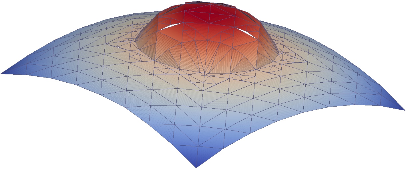
A sketch of a finite element approximation with the locally adapted patch method is given in Figure 10 (b). We note that in contrast to [8], we only split the cut cells into subtriangles for visualization. Thus, there are hanging nodes in the visualization. However, the solution is continuous at these edges. For the presented adapted finite element method we plot the error in the $L^{2}$- and in the $H^{1}$-norm for several levels of global refinement of the mesh in Figure 11. We recover the optimal quadratic convergence for the error in the $L^{2}$-norm and linear convergence in the $H^{1}$-norm as proven in Theorem 1.

Figure 11: Optimal convergence recovered with the adapted finite element method. Solid lines indicate a slope of $h$ and $h^{2}$, respectively.

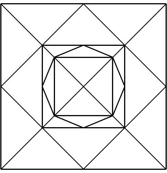
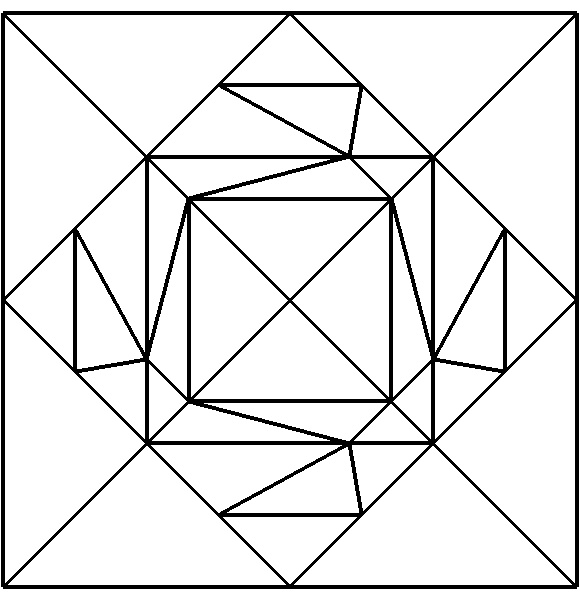
In Figure 12, we present three meshes which arise in the approximation of (20). The subtriangles of the cells which are cut by the interface are shown. In the mesh in Figure 12 (a), the free parameters which are not determined by the cut of the interface are chosen to be $\nicefrac{{1}}{{2}}$. Therefore, the maximum angle condition could be violated. For the other two meshes in Figures 12 (b) and 12 (c), we apply two different strategies for choosing the free parameters. In those meshes, the maximum angle condition will be satisfied.

(a) Strategy 1.

(b) Strategy 2.

(c) Strategy 3.

Figure 12: Cut cells for the approximation of (20) after one level of global refinement of the initial mesh in Figure 10 (a), free parameters chosen after different strategies.

5.2 Horizontal cut

In this example we study the behavior of the locally adapted patch finite element method for patch triangles which get very anisotropic. Let us assume that the domain $\Omega=(-1,1)^{2}$ is cut horizontally into

$$\Omega_{1}(\varepsilon)=\{x\in\Omega|x_{2}<\varepsilon h\}\quad\text{ and }\quad\Omega_{2}(\varepsilon)=\{x\in\Omega|x_{2}>\varepsilon h\},$$

where $h$ is the maximum edge length of a triangle $T$. The analytical solution to the interface problem (1) is chosen as

$$u(x)=\begin{cases}\frac{\kappa_{2}}{\kappa_{1}}(x_{2}-\varepsilon h)-(x_{2}-\varepsilon h)^{2},&x\in\Omega_{1},\\ (x_{2}-\varepsilon h)-(x_{2}-\varepsilon h)^{2},&x\in\Omega_{2}.\end{cases}$$

Figure 13: Error in the $L^{2}$-norm error depending on $\varepsilon$, strategy 1.

The right hand side and the boundary conditions are computed accordingly. The vertical edge length in a patch triangulation will vary due to the value of $\varepsilon$. Vertical edge lengths between $\varepsilon h$ and $(1-\varepsilon)h$ will occur for $\varepsilon\in[0,1]$. Here, $h$ denotes the maximum edge length of a triangle $T$.

Figure 14: Error in the $L^{2}$-norm depending on $\varepsilon$, strategy 2.

We plot the error in the $L^{2}$- and $H^{1}$-norm for different values of $\varepsilon\in[0,1]$ in Figures 13 to 18. As expected and already reported in [8], we observe the smallest errors for $\varepsilon=0$, $\varepsilon=\nicefrac{{1}}{{2}}$, and $\varepsilon=1$, as then the cut is resolved by the mesh.

Figure 15: Error in the $L^{2}$-norm depending on $\varepsilon$, strategy 3.

The largest errors arise for the cases in which $\varepsilon\to 0$ and $\varepsilon\to 1$ since then, the anisotropies for the patch cells become maximal. However, the errors stay bounded. This behavior is similar on finer meshes but the variations get smaller.

Figure 16: Error in the $H^{1}$-norm depending on $\varepsilon$, strategy 1.

Figure 17: Error in the $H^{1}$-norm error depending on $\varepsilon$, strategy 2.

Figure 18: Error in the $H^{1}$-norm depending on $\varepsilon$, strategy 3.

The errors are smaller if we choose the free parameters such that the maximum angle condition will be satisfied. However, the error behaves quite similar for all three strategies to choose the free parameters. There is no significant difference between the error in the $L^{2}$-norm shown in Figures 14 and 15 and the error in the $H^{1}$-norm shown in Figures 17 and 18. For this example, we conclude that it matters to choose the free parameter to satisfy a maximum angle condition. However, it does not seem to matter which of the suggested values to choose.

5.3 Tilted interface line

In this numerical example, we consider a straight interface which cuts the domain $\Omega=(-1,1)^{2}$ in two subdomains

$$\Omega_{1}(\alpha)=\{x\in\Omega|\cos(\alpha)x_{2}<\sin(\alpha)x_{1}\},$$

and

$$\Omega_{2}(\alpha)=\{x\in\Omega|\cos(\alpha)x_{2}>\sin(\alpha)x_{1}\}.$$

Depending on the value of $\alpha$, the straight interface is defined by $\cos(\alpha)x_{2}=\sin(\alpha)x_{1}$. We choose an analytical solution to problem (1) as

$$u(x)=\begin{cases}\sin\big{(}\frac{\kappa_{2}}{\kappa_{1}}(\cos(\alpha)x_{2}-\sin(\alpha)x_{1})\big{)},&x\in\Omega_{1},\\ \sin(\cos(\alpha)x_{2}-\sin(\alpha)x_{1}),&x\in\Omega_{2}.\end{cases}$$

From this exact solution, the right hand side and boundary conditions are computed accordingly. We plot the error in the $L^{2}$- and $H^{1}$-norm for different values of $\alpha\in[0,\pi]$ in Figures 19 to 24.

Figure 19: Error in the $L^{2}$-norm depending on $\alpha$, strategy 1.

Figure 20: Error in the $L^{2}$-norm depending on $\alpha$, strategy 2.

Figure 21: Error in the $L^{2}$-norm depending on $\alpha$, strategy 3.

Figure 22: Error in the $H^{1}$-norm depending on $\alpha$, strategy 1.

Figure 23: Error in the $H^{1}$-norm depending on $\alpha$, strategy 2.

Figure 24: Error in the $H^{1}$-norm depending on $\alpha$, strategy 3.

In this example, the choice of the free parameters does not make any difference. In contrast to the previous example we even get the same behavior of the error if we choose the free parameters to be $\nicefrac{{1}}{{2}}$.

6 Conclusions

We presented an extension of the locally adapted patch finite element method to triangles. In order to resolve a solution at an interface, patch triangles which are cut by the interface are divided into subtriangles. Linear polynomials on these subtriangles together with a local quadrature rule are applied.

Thanks to linear transformations of the subtriangles to the exact location of the cut in the patch triangle, no degrees of freedom have to be moved, inserted or deleted. Thus, this method is perfectly suitable for parallel computing on distributed architectures.

A key ingredient for the a priori error analysis of the locally adapted finite element patch method was the maximum angle condition. In contrast to the locally adapted patch finite element method on quadrilaterals, the maximum angle condition is not automatically satisfied on triangular meshes. We suggested various possibilities to overcome this shortcoming. With these adjustments, the optimal order of convergence for the error in the $L^{2}$- and the $H^{1}$-norm are recovered. This is also shown in the numerical experiments. Furthermore, we observe in the numerical tests that these adjustments are not necessarily leading to a better behavior for the error.

In future research, we plan to parallelize the method and to extend it to three dimensional tetrahedral meshes. Furthermore, we would like to apply our method to time-dependent and more complex problems such as fluid-structure interaction problems.

References

- [1] T. Apel. Anisotropic Finite Elements: Local Estimates and Applications. Advances in Numerical Mathematics. Teubner, Stuttgart, 1999.
- [2] I. Babuška. The finite element method for elliptic equations with discontinuous coefficients. Computing, 5(3):207–213, 1970.
- [3] I. Babuška, U. Banerjee, and J. E. Osborn. Generalized finite element methods – Main ideas, results and perspective. International Journal of Computational Methods, 01(01):67 – 103, 2004.
- [4] J. H. Bramble and J. T. King. A robust finite element method for nonhomogeneous dirichlet problems in domains with curved boundaries. Mathematics of Computation, 63(207):1–17, 1994.
- [5] E. Burman, S. Claus, P. Hansbo, M. G. Larson, and A. Massing. CutFEM: Discretizing geometry and partial differential equations. International Journal for Numerical Methods in Engineering, 104(7):472–501, 2015.
- [6] E. Burman, P. Hansbo, M. G. Larson, and S. Zahedi. Cut finite element methods for coupled bulk–surface problems. Numerische Mathematik, pages 1–29, 2015.
- [7] P. Ciarlet. The Finite Element Method for Elliptic Problems. Studies in Mathematics and its Applications. Elsevier Science, 1978.
- [8] S. Frei and T. Richter. A Locally Modified Parametric Finite Element Method for Interface Problems. SIAM J. Numerical Analysis, 52(5):2315 – 2334, 2014.
- [9] P. Gangl and U. Langer. A Local Mesh Modification Strategy for Interface Problems with Application to Shape and Topology Optimization. ArXiv e-prints, 2016.
- [10] A. Hansbo and P. Hansbo. An unfitted finite element method, based on Nitsche’s method, for elliptic interface problems. Computer Methods in Applied Mechanics and Engineering, 191(47 – 48):5537 – 5552, 2002.
- [11] A. Hansbo and P. Hansbo. A finite element method for the simulation of strong and weak discontinuities in solid mechanics. Computer Methods in Applied Mechanics and Engineering, 193(33 – 35):3523 – 3540, 2004.
- [12] R. J. Mackinnon and G. F. Carey. Treatment of material discontinuities in finite element computations. International Journal for Numerical Methods in Engineering, 24(2):393–417, 1987.
- [13] N. Moës, J. Dolbow, and T. Belytschko. A finite element method for crack growth without remeshing. International Journal for Numerical Methods in Engineering, 46(1):131 – 150, 1999.
- [14] J. Wloka. Partial Differential Equations. Cambridge University Press, 1987.