Reverberation Mapping of Optical Emission Lines in Five Active Galaxies

Abstract

We present the first results from an optical reverberation mapping campaign executed in 2014, targeting the active galactic nuclei (AGN) MCG+08-11-011, NGC 2617, NGC 4051, 3C 382, and Mrk 374. Our targets have diverse and interesting observational properties, including a ”changing look” AGN and a broad-line radio galaxy. Based on continuum-H$\beta$ lags, we measure black hole masses for all five targets. We also obtain H$\gamma$ and Heii $\lambda 4686$ lags for all objects except 3C 382. The Heii $\lambda 4686$ lags indicate radial stratification of the BLR, and the masses derived from different emission lines are in general agreement. The relative responsivities of these lines are also in qualitative agreement with photoionization models. These spectra have extremely high signal-to-noise ratios (100–300 per pixel) and there are excellent prospects for obtaining velocity-resolved reverberation signatures.

1 Introduction

Understanding the interior structure of active galactic nuclei (AGN) has been a major goal of extragalactic astrophysics since their identification as cosmological objects (Schmidt, 1963). The current schematic structure of the central part of an AGN includes three main components: an accretion disk around a super-massive black hole (SMBH), a broad line region (BLR), and an obscuring structure at some distance beyond the BLR. This basic picture accounts for the large luminosities and prominent recombination/excitation lines observed in Seyfert galaxy and quasar spectra (Burbidge, 1967; Weedman, 1977), as well as the dichotomy between Type 1 and Type 2 objects (Lawrence, 1991; Antonucci, 1993).

While this model has qualitatively explained the observational properties of AGN, the details of AGN interior structure remain poorly understood. The basic physics of the accretion disk are probably linked to the magnetorotational instability (Balbus & Hawley, 1998), but it has not been possible to fully simulate an accretion disk and compare with observations (Koratkar & Blaes, 1999; Yuan & Narayan, 2014). It is also unclear if the BLR simply consists of ambient gas near the SMBH, or if it is more directly connected with the accretion process. For example, broad-line emitting gas might correspond to inflowing gas from large scales that feeds the accretion disk, or a portion of the BLR gas may be the result of an outflowing wind driven by radiation pressure from the accretion disk (Collin-Souffrin, 1987; Murray & Chiang, 1997; Elvis, 2000; Proga & Kallman, 2004; Proga & Kurosawa, 2010; Higginbottom et al., 2014; Elitzur & Netzer, 2016). The BLR could instead correspond to the portion of the obscuring structure lying within the dust sublimation radius (Netzer & Laor, 1993; Simpson, 2005; Gaskell et al., 2008; Nenkova et al., 2008; Mor & Netzer, 2012). Other models explore the possibility that the accretion disk, BLR, and obscuring structure are not distinct at all, but different observational aspects of a single structure bound to the central SMBH (e.g., Elitzur & Shlosman 2006; Czerny & Hryniewicz 2011; Goad, Korista, & Ruff 2012).

Reverberation mapping (RM, Blandford & McKee 1982; Peterson 1993, 2014) is an effective way of investigating these scenarios. RM exploits the intrinsic variability of AGN to investigate the matter distribution around the SMBH. The inner parts of the accretion disk emit in the far/extreme UV, providing ionizing photons that drive line emission from BLR gas. As the accretion disk stochastically varies, changes in the continuum flux are reprocessed as line emission by BLR gas after a time delay that corresponds to the light-travel time across the BLR. Measuring this time delay (or “lag”) provides a means of measuring the characteristic size-scale of the line-emitting gas. Similarly, the UV continuum (or X-rays) deposits a small fraction of the accretion luminosity in the outer parts of the accretion disk and obscuring structure. Continuum variations will therefore change the local temperature of these structures, which can drive variable emission at longer continuum wavelengths—the outer part of the accretion disk emits primarily in the optical and the obscuring structure emits in the IR. By measuring any lag between the primary UV signal and light echoes at longer wavelengths, it is possible to “map” the size of the accretion disk and obscuring structure.

Early RM experiments were able to measure or constrain the physical scales of the three primary components: the accretion disk is of order a few light days from the SMBH (e.g., Wanders et al. 1997; Sergeev et al. 2005), the BLR ranges from several light days to a few light months or light years, depending on the AGN luminosity (Wandel et al. 1999; Kaspi et al. 2000; Peterson et al. 2004; Kaspi et al. 2005), and the obscuring structure extends several light months or light years beyond the BLR (Clavel et al., 1989; Oknyanskij & Horne, 2001; Suganuma et al., 2006). More recent RM studies have provided additional details. The detection of continuum lags across the accretion disk provides information about the disk’s temperature gradient, and it appears that the disks are somewhat larger than the predictions from standard models (e.g., Shappee et al. 2014; Edelson et al. 2015; Fausnaugh et al. 2016; McHardy et al. 2016), as also found in microlensing studies of lensed quasars (e.g., Morgan et al. 2010; Blackburne et al. 2011; Mosquera et al. 2013). Mid- to far-IR echoes from the obscuring structure have facilitated investigation of AGN dust properties, and suggest that the obscuring structure is clumpy and has a mixed chemical composition (Kishimoto et al., 2007; Vazquez et al., 2015).

RM of the BLR is of particular importance for AGN studies because velocity information in the broad-line profile combined with the observed time delay provides a well-calibrated estimate of the SMBH mass. Approximately 60 AGN have RM mass measurements (Bentz & Katz, 2015), and this sample anchors the scaling relations used to infer the majority of SMBH masses throughout the universe (e.g., McLure & Dunlop 2004; Vestergaard & Peterson 2006; Trakhtenbrot & Netzer 2012; Park et al. 2013; Mejía-Restrepo et al. 2016, and references therein). New insights into the BLR structure have also become available with velocity-resolved analyses (e.g., Denney et al. 2010; Bentz et al. 2010; Barth et al. 2015; Valenti et al. 2015; Du et al. 2016). By combining information about the BLR time delay as a function of line-of-sight velocity, it is possible to distinguish among geometric and dynamical configurations, such as flattened versus spherical matter distributions and dynamics dominated by rotation, infall, or outflow (Horne, 1994; Horne et al., 2004; Bentz et al., 2010; Grier et al., 2013b; Pancoast et al., 2014a, b). So far, only about 10 AGN have such detailed velocity-resolved results, but they suggest a wide range of dynamics and geometries.

In this work, we present the first results from an intensive RM campaign executed in 2014. This campaign had two primary goals: to measure SMBH masses in several objects with interesting or peculiar observational properties, and to expand the sample of AGN with velocity-resolved reverberation signatures. NGC 5548 was also observed in this campaign as part of the multiwavelength AGN STORM project (De Rosa et al. 2015; Edelson et al. 2015; Fausnaugh et al. 2016; Goad et al. 2016). Ground-based spectroscopic results for this object are presented by Pei et al. (2017). Here, we present the final data and initial analysis of other AGN from this campaign, reporting continuum and line light curves, continuum-line lag measurements, and SMBH masses for five objects. We detected variability in the H$\beta$, H$\gamma$ and Heii $\lambda 4686$ emission lines for most objects, which we also use to explore the photoionization conditions in the BLR (Korista & Goad, 2004; Bentz et al., 2010). These data are of exceptional quality and should allow us recover velocity-resolved reverberation signatures in future work.

In §2, we present our target AGN, observations, data reduction, and light curves. In §3, we explain our time-series analysis and report continuum-line lags. In §4 we measure the gas velocities and estimate SMBH masses. In §5 we discuss our results, and in §6 we summarize our findings. We assume a consensus cosmology with $H_{0}=70{\rm\ km\ s^{-1}\ Mpc^{-1}}$, $\Omega_{\rm m}=0.3$, and $\Omega_{\Lambda}=0.7$.

2 Observations and Data Reduction

2.1 Targets

Table 1: Target Properties

Object	Redshift	$D_{L}$	Number of	$F$ [Oiii]$\lambda$5007	[Oiii]$\lambda$5007	$\log\lambda L_{5100\text{\AA}}$	$\log\lambda L_{\rm host}$	E(B$-$V)
		(Mpc)	Good-weather Epochs	($10^{-14}$ erg cm-2 s-1)	Light Curve Scatter (%)	[erg s-1]	[erg s-1]	(mag)
(1)	(2)	(3)	(4)	(5)	(6)	(7)	(8)	(9)
MCG+08-11-011	0.0205	89.1	6	$61.33\pm 0.21$	0.09	43.59	43.28	0.19
NGC 2617	0.0142	61.5	3	$6.88\pm 0.06$	1.37	43.12	42.95	0.03
NGC 4051	0.0023	17.1	3	$41.30\pm 0.26$	0.36	42.38	42.23	0.01
3C 382	0.0579	258.7	6	$7.87\pm 0.06$	0.92	44.20	43.98	0.06
Mrk 374	0.0426	188.5	3	$7.27\pm 0.11$	0.62	43.98	43.61	0.05

Note. — Column 2 is taken from the NASA Extragalactic Database. Column 3 gives the luminosity distance $D_{L}$ in a concensus cosmology, except for NGC 4051 for which the luminosity distance is from Tully et al. (2008). Column 4 gives the number of nights with clear and stable conditions on which each object was observed. Each object had three observations per night, which were used to calculate the narrow [Oiii]$\lambda$5007 line flux. The line flux and its uncertainty are given in Column 5. Column 6 gives the fractional variation of the [Oiii]$\lambda$5007 line light curve, which serves as an estimate of the night-to-night calibration error (§2.5.1). Column 7 gives the observed luminosity (corrected for Galactic extinction), calculated from the observed 5100 Å rest-frame light curve and Column 3. Column 8 gives the luminosity of the host-galaxy starlight in the spectroscopic extraction aperture, also corrected for Galactic extinction (§5.1). Note that Column 7 includes the contribution from the host galaxy. Column 9 gives the Galactic reddening value from Schlafly & Finkbeiner (2011).

In spring of 2014 we monitored 11 AGN over the course of a six-month RM campaign. The AGN were selected with the aim of expanding the database of RM SMBH masses, particularly for objects with diverse and peculiar observational characteristics. The second goal of our campaign was to investigate the dynamics and geometry of the BLR with velocity-resolved reverberation signatures, i.e., velocity-delay maps and dynamical models (see e.g. Grier et al. 2013b; Pancoast et al. 2014a). Here, we focus on results related to SMBH masses, and we will pursue the velocity-resolved analysis in future work.

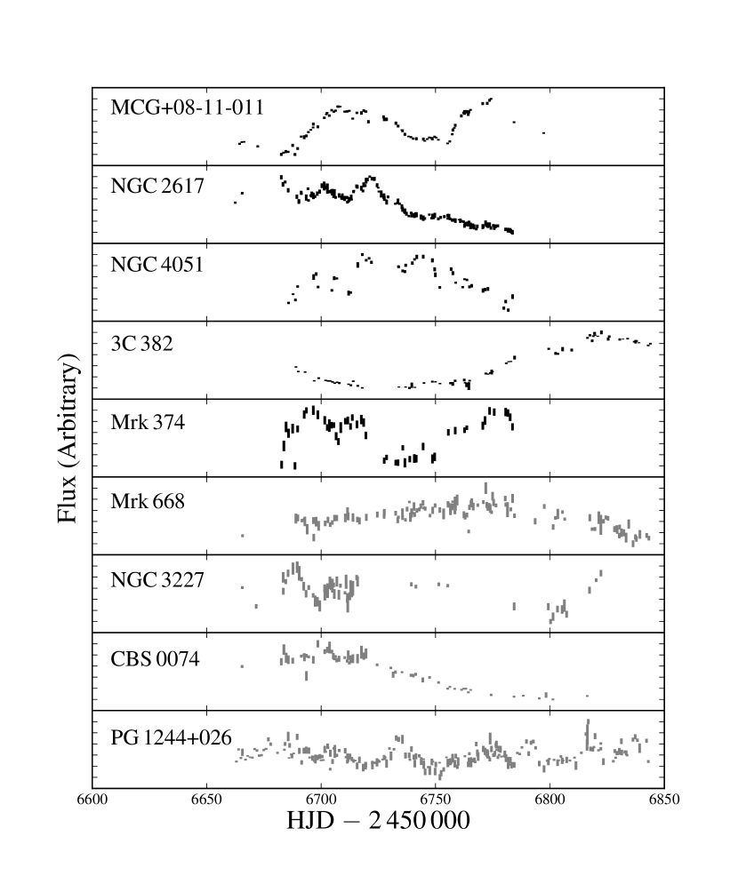
Figure 1 shows g-band light curves from the Las Cumbres Observatory (LCO) 1m network for nine of our targets (we discuss these data in detail in §2.3). Not shown are Akn 120, which was dropped early in the campaign because of low variability, and NGC 5548, for which the results are presented elsewhere (Fausnaugh et al. 2016; Pei et al. 2017). In order to estimate a black hole mass, we must measure a continuum–line lag. We have not been able to measure such a reverberation signal for Mrk 668, NGC 3227, CBS 0074, and PG 1244+026. These sources have lower signal-to-noise ratios (S/Ns) than the other objects (generally 30–70 per pixel, although NGC 3227 was $\sim\!90$ per pixel; see §2.5.3), and they display lower variability amplitudes. The fractional root-mean-square amplitude ($F_{\rm var}$ as defined in §2.5.3 below) is 0.012 for Mrk 668, 0.037 for NGC 3227, 0.010 for CBS 0074, and 0.025 for PG 1244+026. For Mrk 668, the slow rate of change in the light curve also makes it impossible to measure short lags. For NGC 3227, the light curve is problematic because of the limited sampling and large gaps; however, this object was also observed during a monitoring campaign in 2012, and we will combine the data from both campaigns in a future analysis. For CBS 0074 and PG 1244+026, we have not been able to obtain a sufficiently precise calibration of the spectra (see §2.2.2) to detect emission line variability.

We succeeded in measuring black hole masses for MCG+08-11-011, NGC 2617, NGC 4051, 3C 382, and Mrk 374. Table 1 lists the some of the important properties of these objects (several of which are measured in this study), and we provide additional comments as follows:

1. MCG+08-11-011 is a strong X-ray source for which spectral signatures of a relativistically-broadened Fe K$\alpha$ line have been observed with Suzaku (Bianchi et al., 2010). The Fe K$\alpha$ emission is believed to be emitted close to the inner edge of the accretion disk, and can potentially be used to measure the spin parameter of the black hole. Because the black hole mass and spin are to some extent degenerate when fitting the broad Fe K$\alpha$ profile, an independent mass estimate from RM can greatly assist with the spin measurement.

2. NGC 2617 was discovered by Shappee et al. (2014) to be a “changing look” AGN. In 2013, after a large X-ray/optical outburst, follow-up spectroscopic observations showed the presence of broad lines, while archival spectra from 2003 show only a weak broad component of H$\alpha$. This means that the classification of NGC 2617 changed from a Seyfert 1.9 to Seyfert 1.0 sometime in the intervening decade. Few optical “changing look” AGN are known, although systematic searches through long-term survey data (such as the SDSS, LaMassa et al. 2015; MacLeod et al. 2016) and targeted repeat spectroscopy (Runnoe et al., 2016; Runco et al., 2016; Ruan et al., 2016) have recently expanded the sample size to approximately 20 objects, depending on how “changing look” AGN are defined. The absolute rate of this phenomenon is very uncertain, but these recent studies suggest that it may be relatively common over several decades, a time scale that long-term spectroscopic surveys are only beginning to probe. Velocity-resolved dynamical information is of special interest in an object such as this, since the presence of outflows or infall may provide clues about the physical mechanism behind the change in Seyfert category.

3. NGC 4051 has been the target of several optical and X-ray RM campaigns (Shemmer et al., 2003; Peterson et al., 2000, 2004; Denney et al., 2009b; Miller et al., 2010; Turner et al., 2017). However, the short H$\beta$ lag, comparable to the cadence of most monitoring campaigns, has led to mixed and inconsistent results. Denney et al. (2009b) found an H$\beta$ lag of $1.87\pm 0.52$ days, roughly a factor of 2 smaller than previous studies. Because of the large change, as well as the lag’s small value compared to the monitoring cadence, we re-observed NGC 4051 during the 2014 campaign to check this result. For one month of the campaign (2014 February 17 to 2014 March 16 UTC), we also increased the monitoring cadence of NGC 4051 to twice nightly, in order to securely resolve the expected short H$\beta$ lag.

   NGC 4051 is also an archetypal narrow-line Seyfert 1 (NLS1), meaning that the width of its H$\beta$ line is $\lesssim 2\,000{\rm\ km\ s}^{-1}$. There are two competing theories to explain the NSL1 phenomenon: high accretion rates or rotationally-dominated BLR dynamics seen nearly face-on. Both explanations can account for the narrow linewidths given the AGN luminosity. Insight into the structure of the BLR can help distinguish between these explanations, so there is considerable interest in reconstructing a velocity-delay map for this object.

4. 3C 382 is an FR II broad-line radio galaxy (Osterbrock et al., 1975, 1976). Few radio-loud AGN have RM mass measurements, although there are notable examples such as 3C 390 (Shapovalova et al., 2010; Dietrich et al., 2012), 3C 273 (Kaspi et al., 2000; Peterson et al., 2004), and 3C 120 (Peterson et al., 2004; Grier et al., 2012). These objects are typically more luminous than radio-quiet AGN, so they have large lags (of order months to years) that are difficult and expensive to measure. However, radio emission is thought to be associated with more massive black holes, which can be tested by anchoring radio-loud AGN to the RM mass scale. Radio jets can also provide an indirect estimate of the inclination of the BLR, if the BLR is a disky structure with the rotation axis aligned to that of the jet (Wills & Browne 1986). Several jet-orientation indicators exist for 3C 382, and Eracleous et al. (1995) estimated the BLR inclination in 3C 382 using dynamical models of the double-peaked H$\alpha$ profile. Velocity-delay maps and dynamical models would provide an interesting comparison to these estimates.

5. We observed Mrk 374 in an RM campaign from 2012, but the AGN did not display sufficient variability to measure emission line lags at that time. Although Mrk 374 is our least variable source, we succeeded in measuring a line lag from the 2014 campaign, and we present the first RM-based black hole mass here.

Figure 1: g-band light curves of all targets in the 2014 monitoring campaign except for Akn 120 and NGC 5548 (see §2.1). In this study, we focus on MCG+08-11-011, NGC 2617, NGC 4051, 3C 382, and Mrk 374. The extent of the errorbars on the open white circles represent 10% variations for each flux scale.

2.2 Spectra

2.2.1 Observations

We obtained spectra on an approximately daily cadence between 2014 January 04 and 2014 July 06 UTC using the Boller and Chivens CCD Spectrograph on the 1.3m McGraw-Hill telescope at the MDM Observatory. We used the 350 mm^-1 grating, yielding a dispersion of 1.33 Å per pixel with wavelength coverage from 4300 Å to 5600 Å. We kept the position angle of the slit fixed to 0^∘ for the entire campaign, with a slit width of 5$\farcs$0 to minimize losses due to differential refraction and aperture effects caused by extended emission (i.e., the host-galaxy and narrow line region, Peterson et al. 1995). Because of the large slit width, the spectroscopic resolution for point sources (such as the AGN) is limited by the image seeing. We discuss this in more detail in §4, but comparison with high-resolution observations suggest that the effective spectral resolution is approximately 7.0 Å.

The two-dimensional spectra were reduced using standard IRAF tasks for overscan, bias, and flat-field corrections, and cosmic rays were removed using LA-cosmic (van Dokkum, 2001). We extracted one-dimensional spectra from a 15$\farcs$0 window centered on a linear fit to the trace, and we derived wavelength solutions from comparison lamps taken in the evening and morning of all observing nights. We also corrected for zero-point shifts in the wavelength solutions (due to flexure in the telescope) by taking xenon lamp exposures just prior to each observing sequence. However, every AGN was observed for a series of three 20 minute exposures and the wavelength zero-point can drift over the course of this hour, especially at high airmass. We therefore tie the wavelength solution of the first exposure to the contemporaneous xenon lamp, and then apply shifts that align the [Oiii] $\lambda 5007$ emission line of subsequent exposures to that of the first. This procedure results in wavelength solutions accurate to 0.56 Å, as measured from night-sky emission lines.

We applied relative flux calibrations using sensitivity curves derived from nightly observations of standard stars. For most of the campaign, we use Feige 34 (Oke, 1990) to define the nightly sensitivity curve. However, this star began to set near dusk at the end of the campaign, so we tied our relative flux calibration to BD+33^∘2642 (Oke, 1990) for the final two weeks. The change in standard star could potentially result in a systematic change in the observed continuum slopes. However, BD+33^∘2642 and Feige 34 were observed for a one-month overlap period before the transition, and the sensitivity curves derived from both stars agree well during this time period. Of the targets presented here, only 3C 382 was observed during the final two weeks, and we did not find any anomalous changes in the spectral slope during this period. As a check on the relative flux calibration, we also looked for a “bluer when brighter” trend, caused by an increasing fraction of host-galaxy light when the AGN is in a faint state and/or intrinsic variations in the AGN spectral energy distribution (e.g., Wilhite et al. 2005; Sakata et al. 2010). We measured the spectral slope by fitting a straight line to each spectrum with the emission lines masked, and for all cases except the weakly varying Mrk 374, we found a significant anticorrelation between the mean flux and the spectral slope. Detecting the “bluer when brighter” effect lends additional confidence to our relative flux calibration.

We also obtained six epochs of observations with the 2.3m telescope at Wyoming Infrared Observatory (WIRO) and the WIRO Long Slit Spectrograph. The WIRO spectra were used to fill in gaps in the MDM monitoring, and we matched the spectrograph configuration to that of the MDM spectrograph as closely as possible. This includes a 5$\farcs$0 slit at position angle 0^∘ for all observations, and we used the same extraction/sky apertures as for the MDM observations. The wavelength calibrations and spectral slopes of the WIRO data agree well with the MDM observations, and we discuss the calibration of the WIRO data to the MDM flux scale in §2.5.1.

2.2.2 Night-to-Night Flux Calibration

In order to account for variable atmospheric extinction and seeing, we employ the calibration algorithms introduced by Fausnaugh (2017). This approach is similar to the older method of van Groningen & Wanders (1992), but yields markedly better calibrations. We assume that the [Oiii] $\lambda 5007$ emission line is constant over the course of our campaign, and we transform the observed spectra so that their [Oiii] $\lambda 5007$ line profiles match those of the “photometric” nights (nights with clear conditions and stable seeing). We treat the WIRO and MDM spectra separately and inter-calibrate the two flux scales below (§2.5.1).

Fausnaugh (2017) discusses the details of our implementation and provides a python package (mapspec) to build and apply a rescaling model to time-series spectra. For completeness, we briefly outline the procedure here:

1. First, we collected the spectra taken on photometric nights (as judged by the observers onsite) and estimated their [Oiii] $\lambda 5007$ line fluxes. The line fluxes were measured by subtracting a linearly interpolated estimate of the local continuum underneath the line and then integrating the remaining flux using Simpson’s method. We provide the wavelength regions of the integration and the continuum fit in Tables 2 and 3. We applied iterative 3$\sigma$ clipping to the line fluxes, where $\sigma$ is their root-mean-square (rms) scatter, in order to reject any outliers (due to slit losses or anomalies in the sky conditions). We then averaged the remaining flux measurements to estimate the true line flux. The measured [Oiii] $\lambda 5007$ line fluxes for each object are given in Table 1. Table 1 also gives the number of photometric epochs used to determine these fluxes for each AGN (we usually took three spectra per epoch).

2. We then combined the remaining photometric spectra into a reference spectrum using a noise-weighted average. In this step, any residual wavelength shifts were removed by aligning the [Oiii] $\lambda 5007$ line profiles using Markov Chain Monte Carlo (MCMC) methods—the spectra are shifted by the wavelength shift that minimizes the sum of the squares of residuals between the [Oiii] $\lambda 5007$ line profiles. Linear interpolation is used for wavelength shifts of fractional pixels.

3. Due to changes in seeing, spectrograph focus, and small guiding errors, the spectral resolution of each observation is slightly different. To address this, we smooth the reference spectrum with a Gaussian kernel so that the [Oiii] $\lambda 5007$ linewidth matches the largest [Oiii] $\lambda 5007$ linewidth in the time series. The smoothed reference spectrum will define the final resolution of the calibrated spectra.

4. The time-series spectra are then aligned to the reference by matching the [Oiii] $\lambda 5007$ line profiles, again in a least-squares sense using MCMC methods. The differences in line profiles are modeled by a flux rescaling factor, a wavelength shift, and a smoothing kernel. After rescaling, we combine spectra from a single night using a noise-weighted average.

2.3 Imaging

Our spectroscopic observations are supplemented with broad-band imaging observations. Contributing telescopes were the 0.7m at the Crimean Astrophysical Observatory (CrAO), the 0.5m Centurian 18 at Wise Observatory (WC18, Brosch et al. 2008), and the 0.9m at West Mountain Observatory (WMO). CrAO uses an AP7p CCD with a pixel scale of 1$\farcs$76 and a $15^{\prime}\times 15^{\prime}$ field of view, WC18 uses a STL-6303E CCD with a pixel scale of 1$\farcs$47 and a $75^{\prime}\times 50^{\prime}$ field of view, and WMO uses a Finger Lakes PL-3041-UV CCD with a pixel scale of 0$\farcs$61 and a field of view of $21^{\prime}\times 21^{\prime}$. Fountainwood Observatory (FWO) also provided observations of NGC 4051 with a 0.4m telescope using an SBIG 8300M CCD. The pixel scale of this detector is 0$\farcs$35 and the field of view is $19^{\prime}\times 15^{\prime}$. All observations were taken with the Bessell V-band.

In addition, we obtained ugriz imaging with the LCO 1m network (Brown et al., 2013), which consists of nine identical 1m telescopes at four observatories spread around the globe. These data were originally acquired as part of LCO’s AGN Key project (Valenti et al., 2015). The main goal is to search for continuum reverberation signals, which we will pursue in a separate study (Fausnaugh et al., in preparation). However, 3C 382 and Mrk 374, which are our faintest sources, had low variability amplitudes and poorer S/Ns, so we included the LCO g-band data in the continuum light curves of these objects. Each LCO telescope has the same optic system and detectors—at the time of the RM campaign, the detectors were SBIGSTX-16803 cameras with a field of view of $16^{\prime}\times 16^{\prime}$ and a pixel scale of $0\farcs 23$.

We analyzed the imaging data using the image subtraction software (ISIS) developed by Alard & Lupton (1998). Images were first uploaded to a central repository and vetted by eye for obvious reduction errors or poor observing conditions. We then registered the images to a common coordinate system and constructed a high S/N reference frame by combining the best-seeing and lowest-background images. When combining, ISIS adjusts the images to a common seeing by convolving the point-spread function (PSF) of each image with a spatially variable kernel. Finally, we subtracted the reference frame from each image, again allowing ISIS to match the PSFs using its convolution routine. Reference images and subtractions for each telescope/filter/detection system were constructed separately—we discuss combining the photometric measurements in §2.5.2.

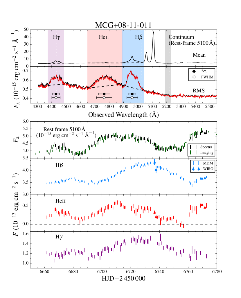
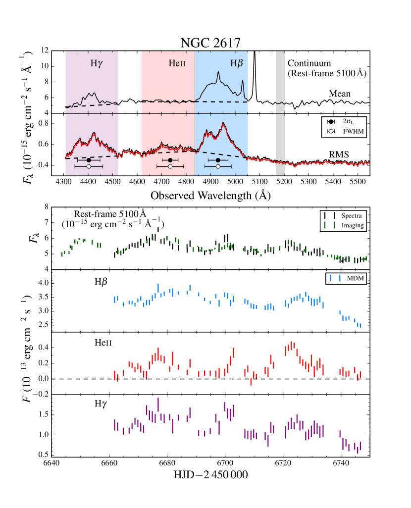
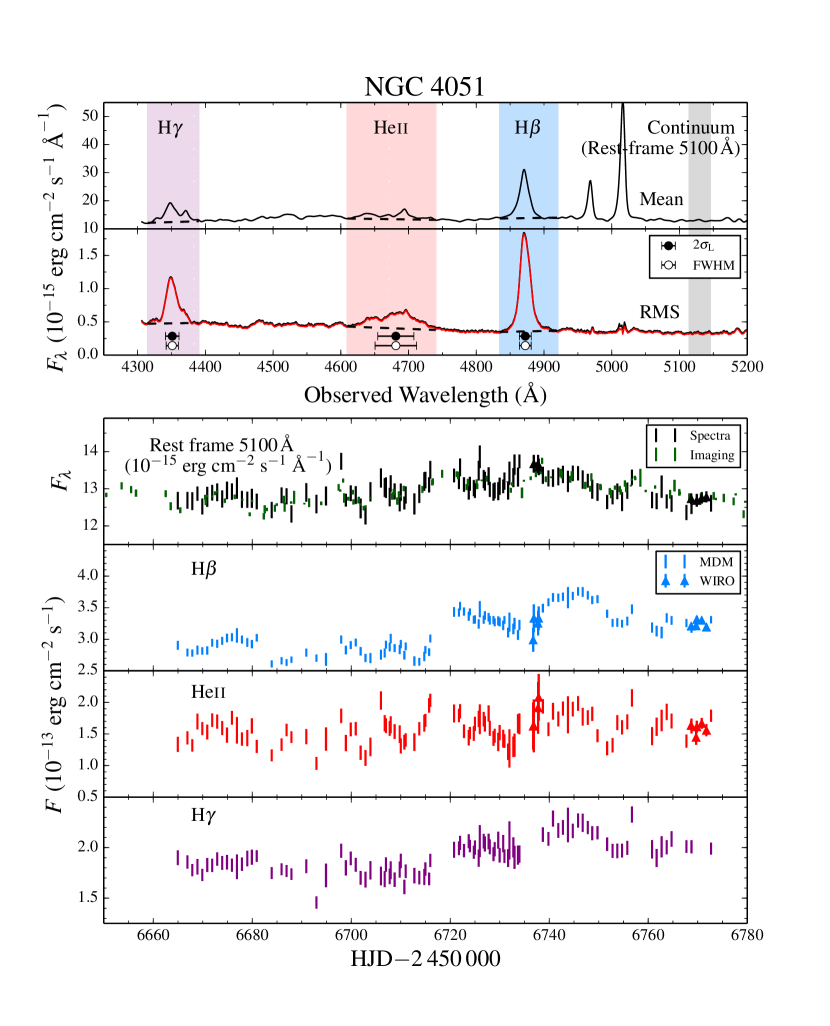
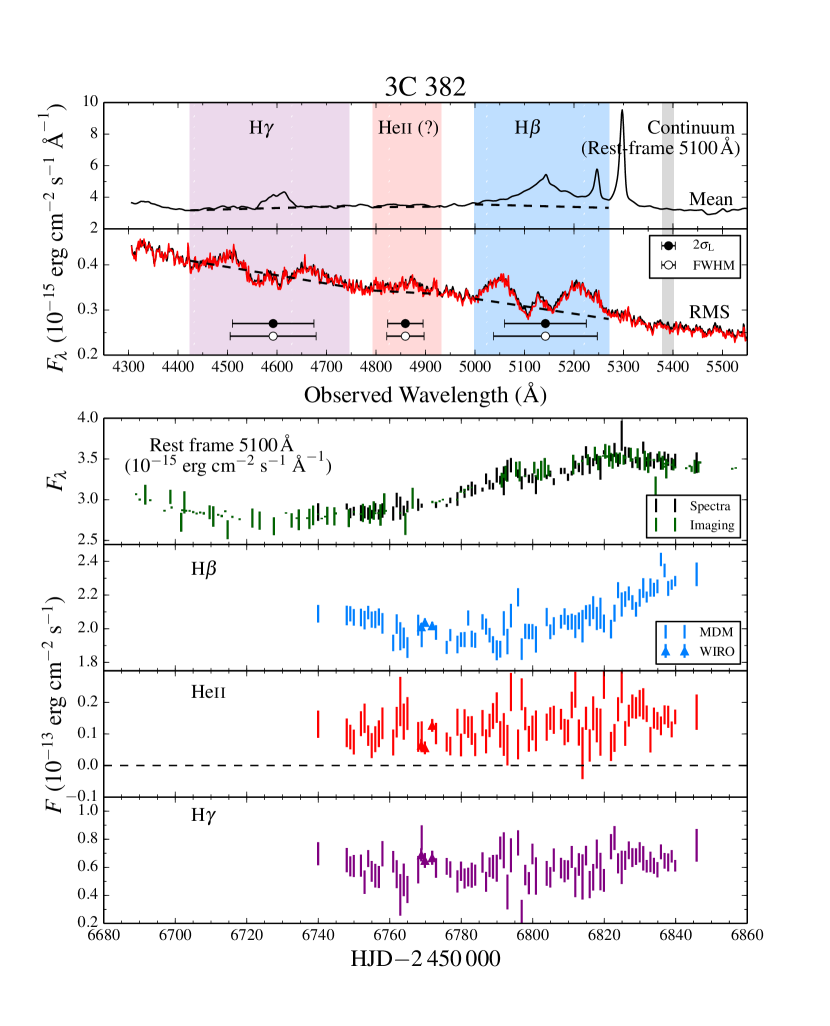
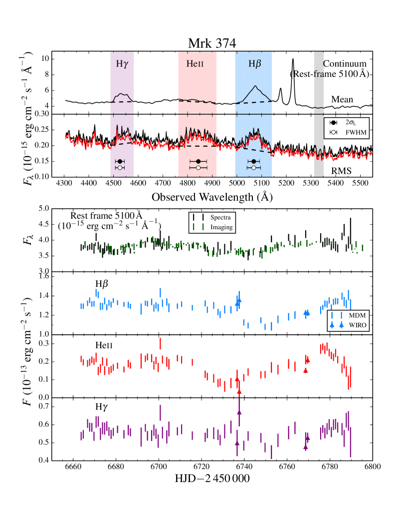
2.4 Mean and rms spectra

Figures 2–6 show the noise-weighted mean spectrum

$$\overline{F}(\lambda)=\frac{\sum_{i=1}^{N_{t}}F(\lambda,t_{i})/\sigma^{2}(\lambda,t_{i})}{\sum_{i=1}^{N_{t}}1/\sigma^{2}(\lambda,t_{i})}$$ (1)

for each object using the MDM observations, where $F(\lambda,t_{i})$ is the flux density at epoch $t_{i}$ and $\sigma(\lambda,t_{i})$ is its uncertainty. Figures 2–6 also show root-mean-square (rms) residual spectra, defined as

$$\sigma_{\rm rms}(\lambda)=\sqrt{\frac{1}{N_{t}-1}\sum_{i=1}^{N_{t}}\left[F(\lambda,t_{i})-\overline{F}(\lambda)\right]^{2}}.$$ (2)

By the Wiener-Khinchin theorem, this statistic is proportional to the integrated variability power at each wavelength, so $\sigma_{\rm rms}$ is free of constant contaminants such as host-galaxy and narrow emission line flux. However, the total variability power contains contributions from both intrinsic variations and from statistical fluctuations/measurement uncertainties. In order to separate these components, we use a maximum-likelihood method (cf. Park et al. 2012b; Barth et al. 2015; De Rosa et al. 2015). We solve for the intrinsic variability $\sigma_{\rm var}(\lambda)$ that minimizes the negative log-likelihood

$$-2\ln\mathcal{L}=\sum_{i=1}^{N_{t}}\frac{\left[F(\lambda,t_{i})-\hat{F}(\lambda)\right]^{2}}{\sigma^{2}(\lambda,t_{i})+\sigma_{\rm var}^{2}(\lambda)}$$

$$+\sum_{i=1}^{N_{t}}\ln\left[\sigma^{2}(\lambda,t_{i})+\sigma_{\rm var}^{2}(\lambda)\right]$$ (3)

where $\hat{F}(\lambda)$ is the “optimal average” weighted by $\sigma^{2}(t_{i})+\sigma^{2}_{\rm var}$. We self-consistently fit for $\hat{F}(\lambda)$ while solving for $\sigma_{\rm var}(\lambda)$, and we show the estimate of $\sigma_{\rm var}(\lambda)$ with the red lines in Figures 2–6. In the limit that $\sigma(\lambda,t_{i})\rightarrow 0$, it is clear that $\sigma_{\rm var}$ is equivalent to $\sigma_{\rm rms}$. For high S/N data such as these, $\sigma_{\rm var}(\lambda)$ is nearly equal to $\left[\sigma_{\rm rms}^{2}(\lambda)-\overline{\sigma}^{2}(\lambda)\right]^{1/2}$, where $\overline{\sigma}^{2}(\lambda)$ is the average of the squared measurement uncertainties across the time-series:

$$\overline{\sigma}^{2}(\lambda)=\frac{1}{N}\sum_{i=1}^{N_{t}}\sigma^{2}(\lambda,t_{i}).$$ (4)

The overall effect is to reduce the squared amplitude of the variability spectrum by the mean squared measurement uncertainty—in all objects except for Mrk 374, this effect is negligible.

2.5 Light curves

Table 2: Observed-frame Integration Windows

Object	5100 Å	H$\beta$	H$\gamma$	Heii$\lambda$4686	[Oiii]$\lambda$5007	[Oiii]$\lambda$4959
	(Å)	(Å)	(Å)	(Å)	(Å)	(Å)
MCG+08-11-011	5190–5230	4890–5040	4375–4485	4650–4890	5085–5130	5040–5075
NGC 2617	5170–5200	4835–5050	4310–4520	4620–4835	5055–5093	5010–5040
NGC 4051	5115–5145	4835–4920	4315–4390	4610–4740	5000–5045	4955–4977
3C 382	5380–5400	5000–5270	4425–4745	4795–4930	5275–5330	5228–5257
Mrk 374	5315–5350	4995–5140	4490–4580	4765–4915	5205–5245	5160–5187

Table 3: Observed-frame Continuum Fitting Windows

Object	Line Side	H$\beta$	H$\gamma$	Heii$\lambda$4686	[Oiii]$\lambda$5007	[Oiii]$\lambda$4959
		(Å)	(Å)	(Å)	(Å)	(Å)
MCG+08-11-011	Blue	4860–4890	4360–4375	4620–4650	5075–5085	5030–5040
	Red	5130–5150	4485–4500	4860–4880	5130–5150	5075–5085
NGC 2617	Blue	4820–4835	4300–4310	4585–4620	5050–5055	5000–5010
	Red	5110–5150	4520–4535	4820–4835	5093–5098	5040–5050
NGC 4051	Blue	4800–4835	4300–4315	4605–4615	4990–5000	4945–4955
	Red	4920–4950	4390–4400	4740–4775	5045–5055	4977–4990
3C382	Blue	4975–5000	4410–4425	4785–4795	5265–5275	5218–5228
	Red	5385–5425	4745–4760	4930–4940	5330–5340	5257–5271
Mrk 374	Blue	4970–4990	4455–4490	4690–4765	5190–5205	5150–5160
	Red	5140–5160	4580–4600	4915–5000	5245–5255	5187–5195

Table 4: Light-curve Properties

Object	Light curve	$N_{t}$	$\Delta t_{\rm med}$	Uncertainty	$\bar{F}$	$\langle{\rm S/N}\rangle$	$F_{\rm var}$	${\rm(S/N)_{var}}$	$r_{\rm max}$
			(days)	Rescaling Factor
(1)	(2)	(3)	(4)	(5)	(6)	(7)	(8)	(9)	(10)
MCG+08-11-011	5100 Å	190	0.59	1.51	4.49	71.2	0.10	67.4	$\equiv 1$
	H$\beta$	86	1.01	1.58	3.79	103.1	0.07	47.8	$0.90\pm 0.01$
	H$\gamma$	82	1.01	1.52	1.29	34.2	0.09	19.2	$0.84\pm 0.03$
	Heii$\lambda$4686	86	1.01	1.46	0.31	6.8	0.44	19.6	$0.78\pm 0.04$
NGC 2617	5100 Å	161	0.92	1.81	5.17	57.2	0.09	44.4	$\equiv 1$
	H$\beta$	61	1.01	1.91	3.31	39.5	0.10	21.1	$0.61\pm 0.07$
	H$\gamma$	61	1.01	1.65	1.18	11.0	0.20	12.3	$0.62\pm 0.07$
	Heii$\lambda$4686	61	1.01	1.18	0.15	3.2	0.61	10.9	$0.49\pm 0.08$
NGC 4051	5100 Å	270	0.47	1.00	12.90	191.7	0.02	49.7	$\equiv 1$
	H$\beta$	107	0.96	3.42	3.14	45.7	0.09	31.1	$0.59\pm 0.05$
	H$\gamma$	98	0.99	2.48	1.92	26.1	0.08	13.7	$0.50\pm 0.06$
	Heii$\lambda$4686	107	0.96	3.25	1.59	12.9	0.11	10.2	$0.47\pm 0.07$
3c382	5100 Å	209	0.56	1.17	3.18	148.5	0.09	131.3	$\equiv 1$
	H$\beta$	81	1.00	1.70	2.06	43.4	0.05	14.5	$0.83\pm 0.25$
	H$\gamma$	81	1.00	1.66	0.60	8.1	0.07	3.6	$0.59\pm 0.24$
	Heii$\lambda$4686	81	1.00	1.90	0.13	3.2	0.19	3.9	$0.61\pm 0.47$
Mrk 374	5100 Å	180	0.59	2.39	3.80	94.5	0.03	25.5	$\equiv 1$
	H$\beta$	67	1.01	1.54	1.29	38.4	0.05	11.2	$0.50\pm 0.07$
	H$\gamma$	67	1.01	1.79	0.56	18.7	0.04	3.8	$0.42\pm 0.07$
	Heii$\lambda$4686	67	1.01	1.41	0.18	8.2	0.25	11.9	$0.56\pm 0.06$

Note. — Column 3 gives the number of observations in each light curve. Column 4 gives the median cadence. Column 5 gives the rescaling factor by which the statistical uncertainties are multiplied to account for additional systematic errors (see §2.5.1). Column 6 gives the mean flux level of each light curve. The rest-frame 5100 Å continuum light curves are in units of $10^{-15}$ erg cm^-2 s^-1 Å^-1, and the emission line light curves are in units of $10^{-13}$ erg cm^-2 s^-1. Column 7 gives the mean signal-to-noise ratio $\langle{\rm S/N}\rangle$. Column 8 gives the rms fractional variability defined in Equation 6. Column 9 gives the approximate S/N at which we detect variability (see §2.5.3). Column 10 gives the maximum value of the interpolated cross correlation function (see §3.1).

2.5.1 Spectroscopic Light Curves

We extracted spectroscopic light curves for the wavelength windows listed in Table 2 for each AGN. We chose these windows based on visual inspection of the variable line profiles in the $\sigma_{\rm var}(\lambda)$ spectra, with the main goal of capturing the strongest variations in the lines. For 3C 382, the component tentatively identified as Heii $\lambda 4686$ is blue-shifted by almost 100 Å relative to the systematic redshift, and if variable Heii $\lambda 4686$ has a similar profile as the Balmer lines in this object, this component corresponds to the blue wing of the line.

The rest-frame 5100 Å continuum, which is relatively free of emission/absorption lines, was estimated by averaging the flux density in the listed wavelength region. Emission-line fluxes were determined in the same way as for the [Oiii] $\lambda 5007$ line. First we subtracted a linear least-squares fit to the local continuum underneath the emission line. Wavelength regions for the continuum fits are given in Table 3. Then we integrated the remaining flux using Simpson’s method (we did not assume a functional form for the emission line). In cases where the broad H$\beta$ wing extends underneath [Oiii]$\lambda$4959, we subtracted the narrow emission line (again with a local linear approximation of the underlying flux) before integrating the broad line. We did not attempt to separate the narrow components of H$\beta$ and H$\gamma$ from the broad components. These narrow components act as constant flux-offsets for the light curves.

The continuum estimates can lead to significant systematic uncertainties, because the continuum-fitting windows may be contaminated by broad-line wing emission, and the local linearly interpolated continuum may leave residual continuum flux to be included in the line profile. Both of these effects can introduce spurious correlations between the continuum and line light curves, which may biased the final lag estimates. Because we use the $\sigma_{\rm var}(\lambda)$ spectra to select the line and continuum windows, variability in the line wings probably does not have a large impact on our results, and we have found the the resulting light curves (and their lags) are robust to five to ten angstrom changes in the continuum and line windows. Larger shifts, especially as the continuum fitting windows move further from the lines, can result in significantly different lags (of order three times the statistical uncertainties). Full spectral decompositions may be able to address this issue in future studies (see Barth et al. 2015 for a detailed discussion). We discuss these systematic uncertainties further in §4.

After we extracted line fluxes from the WIRO and MDM spectra, we combined the measurements by forcing the light curves to be on the same flux scale. We used the mean MDM [Oiii] $\lambda 5007$ line to define this scale, and multiplied the WIRO line fluxes so that the mean value matched that of MDM. A more sophisticated inter-calibration model would include an additive offset, to account for different amounts of host-galaxy starlight in the MDM and WIRO spectra. However, with the limited amount of WIRO data, additional calibration parameters cannot be well-constrained, and we found the simple multiplicative approach to be adequate. The required rescaling factors were 1.21 for MCG+08-11-011, 1.14 for NGC 4051, 1.09 for 3C 382, and 1.73 for Mrk 374. Weather at WIRO prevented observations of NGC 2617.

The statistical uncertainty on the continuum flux was estimated from the standard deviation within the wavelength region,

$$\sigma(t_{j})=\sqrt{\frac{1}{N_{\lambda}-1}\sum_{i=1}^{N_{\lambda}}\left[F(\lambda_{i},t_{j})-\overline{F}(t_{j})\right]^{2}},$$ (5)

where $\overline{F}(t_{j})$ is the evenly-weighted average flux density at epoch $t_{j}$. Uncertainties on the line light curves were estimated using a Monte Carlo approach: we perturbed the observed spectrum with random deviates scaled to the uncertainty at each wavelength, subtracted a new estimate of the underlying continuum (and the narrow [Oiii] $\lambda 4959$ line when appropriate), and re-integrated the line flux. The deviates were drawn from the multivariate normal distribution defined by the covariance matrix of the rescaled spectrum—these covariances can affect the statistical uncertainty by a factor of two or more (see Fausnaugh 2017 for more details). We repeated this procedure $10^{3}$ times and took the central 68% confidence interval of the output flux distributions as an estimate of the statistical uncertainty.

Because the integrated [Oiii] $\lambda 5007$ line flux is not explicitly forced to be equal from night to night, the scatter of the [Oiii] $\lambda 5007$ line light curve serves as an estimate of our calibration uncertainty (Barth et al., 2015). We extracted narrow [Oiii] $\lambda 5007$ line light curves in the same way as for the broad lines, and the results are shown in Figure 7. Several points are noticeably below the means of their light curves, particularly for NGC 2617 and 3C 382. These observations were taken in poor weather, and display significant scatter between the individual rescaled exposures prior to averaging. This suggests variable amounts of flux-losses between the AGN and extended [Oiii] $\lambda 5007$/host-galaxy, due to variable seeing and large guiding errors that move the object in the slit. Although the rescaling model from §2.2.2 cannot correct this issue, the offsets of these points are not very large compared to the statistical uncertainties (no more than 3.1$\sigma$), and we opt to include them in the analysis. Since the effect due to spatially extended [Oiii] $\lambda 5007$ emission is relatively small even in very poor conditions, it will be unimportant in good conditions.

The fractional standard deviations of the narrow line light curves are given in Table 1 and range between 0.1% and 1.4%. These values only represent our ability to correct for extrinsic variations (such as weather conditions) in the observed spectra. Additional systematic uncertainties dominate the epoch-to-epoch uncertainties of the light curves, including (but not limited to) the nightly sensitivity functions, continuum subtraction, and additional spectral components such as Feii emission. The latter two issues are especially problematic for the Heii $\lambda 4686$ light curves.

To account for these systematics, we rescaled the light curve uncertainties so that they approximate the observed flux variations from night to night. We selected three adjacent points $F(t_{j-1})$, $F(t_{j})$, and $F(t_{j+1})$, linearly interpolated between $F(t_{j-1})$ and $F(t_{j+1})$, and measure $\Delta=[F(t_{j})-I(t_{j})]/\sigma(t_{j})$ where $I(t_{j})$ is the interpolated value at $t_{j}$ and $\sigma(t_{j})$ is the statistical uncertainty on $F(t_{j})$. The deviate $\Delta$ therefore measures the departure of the light curve from a simple linear model. We calculated $\Delta$ for $j=2$ to $N_{t}-1$ (i.e, ignoring the first and last points), and we multiplied the statistical uncertainties $\sigma(t_{j})$ by the mean absolute deviation (MAD) $\overline{|\Delta|}$. We also imposed a a minimum value of 1.0 on these rescaling factors. Inspection of the distribution of $\Delta$ shows that the residuals are reasonably (but not perfectly) represented by a Gaussian with a similar MAD value. This method ensures that the uncertainties account for any systematics that the rescaling model cannot capture. We have ignored the uncertainty in the interpolation $I(t_{j})$, so our method slightly overestimates the required rescaling factors. Monte Carlo simulations may be able to assess the importance of uncertainty in $I(t_{j})$ for future work. The rescaling factors are given in Table 4 and are fairly small, generally running between 1.0 and 2.0, with a mean of 1.8 and a maximum of 3.42 for the H$\beta$ light curve in NGC 4051. NGC 4051 has the largest rescaling factors overall, which may be due to real short time-scale variability that departs from our simple linear model (Denney et al., 2010). We therefore also experimented with using the unscaled light curve uncertainties in our time-series analysis (§3) for this object. We found that our results do not sensitively depend on the scale of the uncertainties, although our Bayesian lag analysis (§3.2) indicates that the unscaled uncertainties are probably underestimated.

2.5.2 Broad-Band Light Curves

Differential photometric light curves were extracted from the subtracted broad-band images using ISIS’s built-in photometry package. The software performs PSF photometry by fitting a model to the reference frame PSF and convolving this model with the kernel that was fitted during image subtraction. Because this transformation accounts for variable seeing, while the image subtraction has removed sources of constant flux, the output light curves cleanly isolate intrinsic variations of the AGN from contaminants such as host-galaxy starlight and seeing-dependent aperture effects. Any other constant systematic errors are also automatically subtracted out of the differential light curves. However, ISIS accounts for only the local Poisson uncertainty from photon-counting, while there are also systematic errors from imperfect subtractions (e.g., Hartman et al. 2004). We addressed this problem in the same way as Fausnaugh et al. (2016). We inspected the differential light curves of comparison stars, and rescaled the uncertainties by a time dependent factor to make the comparison star residuals consistent with a constant model. The reduced $\chi^{2}$ of the comparison star light curves is therefore set to one, which requires an average error rescaling factor of 1.0 to 5.0, depending on the object and the telescope. Since our targets are fairly bright, the formal ISIS uncertainties are very small and rescaling even by a factor of five results in uncertainties no greater than 3–6%. See §2.2 of Fausnaugh et al. (2016) for more details.

We next calibrated the differential broad-band light curves to the flux scale of the spectroscopic continuum light curve. The inter-calibration procedure solves for a maximum-likelihood shift and rescaling factor for each differential light curve, forcing the V-band photometry to match the rest-frame 5100 Å continuum flux. The inter-calibration parameters account for the different detector gains/bias levels, telescope throughputs, and (to first-order) a correction for the wider bandpass and different effective wavelengths of the broad-band filters compared to the spectroscopic-continuum averaging window. An advantage of this procedure is that it does not require accurate knowledge of the image zeropoints (or color corrections), which would otherwise limit the overall precision when combining data from different telescopes. The model also minimizes systematic errors that can result in strong correlations between measurements from the same telescope.

Because observations from various telescopes are never simultaneous, it is necessary to interpolate the light curves when fitting the inter-calibration parameters. We followed Fausnaugh et al. (2016) and modeled the time-series as a damped random walk (DRW), as implemented by the JAVELIN software (Zu et al., 2011). Although recent studies have shown that the power spectra of AGN light curves on short time scales may be somewhat steeper than a DRW (Edelson et al., 2014; Kasliwal et al., 2015), Zu et al. (2013) found that the DRW is an adequate description of the time scales considered here (see also Skielboe et al. 2015; Fausnaugh et al. 2016; Kozłowski 2016a, b). Our interpolation scheme and fitting procedure are identical to those described by Fausnaugh et al. (2016).

2.5.3 Light-curve Properties

The final light curves are shown in Figures 2–6 and given in Tables 5–14. We characterize the statistical properties of the light curves in Table 4, reporting the median cadence, mean flux-level, and average S/N. We also measure the light curve variability using a technique similar to our treatment of the variability spectra $\sigma_{\rm var}(\lambda)$. In the presence of noise, it is necessary to separate the intrinsic variability from that due to measurement errors. We therefore define the intrinsic variability of the light curves as $\sigma_{\rm var}$ and solve for it by minimizing

$$-2\ln\mathcal{L}=\sum_{i}^{N_{t}}\frac{\left[F(t_{i})-\hat{F}\right]^{2}}{\sigma^{2}(t_{i})+\sigma_{\rm var}^{2}}+\sum_{i}^{N_{t}}\ln\left[\sigma^{2}(t_{i})+\sigma_{\rm var}^{2}\right],$$ (6)

where $F(t_{i})$ is the flux at epoch $i$, $\sigma(t_{i})$ is its uncertainty, and $\hat{F}$ is the optimal average flux (weighted by $\sigma^{2}(t_{i})+\sigma^{2}_{\rm var}$). For small measurement uncertainties, the fractional variability $\sigma_{\rm var}/\hat{F}$ converges to the standard definition of the “excess variance” (Rodríguez-Pascual et al., 1997)

$$F_{\rm var}=\frac{1}{\overline{F}}\sqrt{\frac{1}{N-1}\sum_{i}^{N}\left[F(t_{i})-\overline{F}\right]^{2}-\overline{\sigma}^{2}}$$ (7)

where $\overline{\sigma}$ is the time-averaged measurement uncertainty of the light curve. We therefore define $F_{\rm var}=\sigma_{\rm var}/\hat{F}$, and report these values in Table 4. These values are slightly underestimated, since $\hat{F}$ is not corrected for constant components (such as host-galaxy starlight or narrow line emission). We also approximate the S/N of the variability as

$${\rm(S/N)_{var}}=\frac{\sigma_{\rm var}}{\overline{\sigma}\sqrt{2/N_{\rm obs}}}.$$ (8)

The $\sqrt{2/N_{\rm obs}}$ term enters because the variance of $\overline{\sigma}$ is expected to approximately scale as that of a reduced $\chi^{2}$ distribution. However, this calculation assumes uncorrelated uncertainties, and a full analysis requires treatment of the red-noise properties of the light curve (see Vaughan et al. 2003).

With the exception of the 3C 382 H$\gamma$, the 3C 382 Heii $\lambda 4686$, and the Mrk 374 H$\gamma$ light curves, we detect variability in all of the other emission lines at greater than $\sim\!10\sigma$. The variability amplitudes of MCG+08-11-011 and NGC 2617 are especially strong ($F_{\rm var}\gtrsim 10\%$). For NGC 4051, the continuum has little fractional variability ($F_{\rm var}=2\%$), which may be caused by a high fraction of host-galaxy starlight. For MCG+08-11-011, NGC 2617, and NGC 4051, the median cadence is near 1 day for all light curves, and the mean S/N usually ranges from several tens to hundreds. In fact, the S/N in the spectra is even higher, reaching 100 to 300 per pixel in the continuum. Combined with the large variability amplitudes, it likely that we will be able to construct velocity-delay maps and dynamical models for these objects in future work.

Table 5: MCG+08-11-011 Continuum Light Curve

HJD	$F_{\lambda}$	Telescope ID
(days)	($10^{-15}$  ergs s-1 cm-2 Å-1)
(1)	(2)	(3)
6639.5218	$3.6279\pm 0.0448$	CrAO
6649.4750	$3.6413\pm 0.0845$	CrAO
6653.4973	$3.8005\pm 0.0631$	CrAO
6656.3942	$3.9176\pm 0.0425$	CrAO
6661.6986	$3.9866\pm 0.0764$	MDM
6662.2042	$3.9837\pm 0.0412$	WC18
…	…	…

Note. — Column 1 gives HJD $-$ 2 450 000 at mid-exposure. Column 2 give the continuum flux density and uncertainty. Column 3 identifies the contributing telescope (see §2.3). A machine-readable version of this table is published in the electronic edition of this article. A portion is shown here for guidance regarding its form and content.

Table 6: NGC 2617 Continuum Light Curve

HJD	$F_{\lambda}$	Telescope ID
(days)	($10^{-15}$ ergs s-1 cm-2 Å-1)
(1)	(2)	(3)
6639.6747	$4.6776\pm 0.1089$	CrAO
6643.6320	$4.9717\pm 0.1357$	CrAO
6644.5145	$5.0946\pm 0.0871$	CrAO
6646.0981	$5.0904\pm 0.0892$	WC18
6646.5287	$5.4647\pm 0.0885$	CrAO
6647.0990	$5.3930\pm 0.1254$	WC18
…	…	…

Note. — Columns are the same as in Table 5. A machine-readable version of this table is published in the electronic edition of this article. A portion is shown here for guidance regarding its form and content.

Table 7: NGC 4051 Continuum Light Curve

HJD	$F_{\lambda}$	Telescope ID
(days)	($10^{-15}$ ergs s-1 cm-2 Å-1)
(1)	(2)	(3)
6645.6113	$12.7318\pm 0.0624$	WC18
6646.6098	$12.8314\pm 0.0668$	WC18
6647.6275	$13.0803\pm 0.0683$	WC18
6648.5919	$12.9598\pm 0.0499$	WC18
6650.5178	$12.8375\pm 0.0550$	WC18
6653.5959	$13.0814\pm 0.0956$	WC18
…	…	…

Note. — Columns are the same as in Table 5. A machine-readable version of this table is published in the electronic edition of this article. A portion is shown here for guidance regarding its form and content.

Table 8: 3C 382 Continuum Light Curve

HJD	$F_{\lambda}$	Telescope ID
(days)	($10^{-15}$ ergs s-1 cm-2 Å-1)
(1)	(2)	(3)
6670.6411	$3.2490\pm 0.1390$	WC18
6689.0237	$3.0685\pm 0.0094$	LCOGT1
6690.0279	$3.0018\pm 0.0105$	LCOGT1
6691.6169	$3.0619\pm 0.1197$	WC18
6693.0025	$2.9948\pm 0.0106$	LCOGT1
6696.9897	$2.8652\pm 0.0094$	LCOGT1
…	…	…

Note. — Columns are the same as in Table 5. A machine-readable version of this table is published in the electronic edition of this article. A portion is shown here for guidance regarding its form and content.

Table 9: Mrk 374 Continuum Light Curve

HJD	$F_{\lambda}$	Telescope ID
(days)	($10^{-15}$ ergs s-1 cm-2 Å-1)
(1)	(2)	(3)
6663.7432	$3.7706\pm 0.1030$	MDM
6664.7221	$3.7776\pm 0.0649$	MDM
6665.5588	$3.8676\pm 0.1114$	WC18
6666.7292	$3.7496\pm 0.0791$	MDM
6667.7164	$3.7902\pm 0.0850$	MDM
6668.7316	$3.8045\pm 0.1097$	MDM
…	…	…

Note. — Columns are the same as in Table 5. A machine-readable version of this table is published in the electronic edition of this article. A portion is shown here for guidance regarding its form and content.

Table 10: MCG+08-11-011 Line Light Curves

HJD	H$\beta$	H$\gamma$	Heii	Telescope ID
(days)	($10^{-13}$ erg s-1 cm-2)
(1)	(2)	(3)	(4)	(5)
6661.6986	$3.4660\pm 0.0288$	$0.0298\pm 0.0298$	$0.1923\pm 0.0416$	MDM
6663.6924	$3.4891\pm 0.0302$	$0.0291\pm 0.0291$	$0.2341\pm 0.0401$	MDM
6664.6734	$3.4978\pm 0.0346$	$0.0326\pm 0.0326$	$0.2352\pm 0.0407$	MDM
6666.6277	$3.4723\pm 0.0387$	$0.0388\pm 0.0388$	$0.3973\pm 0.0505$	MDM
6667.6147	$3.5429\pm 0.0365$	$0.0354\pm 0.0354$	$0.4047\pm 0.0471$	MDM
6668.6285	$3.5031\pm 0.0307$	$0.0333\pm 0.0333$	$0.3580\pm 0.0437$	MDM
…	…	…	…	…

Note. — Column 1 gives HJD $-$ 2 450 000 at mid-exposure. Columns 2–4 give the line fluxes and their uncertainties. Column 5 identifies the contributing telescope (see §2.3). A machine-readable version of this table is published in the electronic edition of this article. A portion is shown here for guidance regarding its form and content.

Table 11: NGC 2617 Line Light Curves

HJD	H$\beta$	H$\gamma$	Heii	Telescope ID
(days)	($10^{-13}$ erg s-1 cm-2)
(1)	(2)	(3)	(4)	(5)
6661.8270	$3.4179\pm 0.1151$	$1.2480\pm 0.1362$	$0.0439\pm 0.0614$	MDM
6662.8456	$3.4662\pm 0.0848$	$1.2049\pm 0.1039$	$0.0145\pm 0.0470$	MDM
6664.8143	$3.2528\pm 0.0756$	$1.0938\pm 0.0892$	$0.0779\pm 0.0370$	MDM
6666.8417	$3.3192\pm 0.0635$	$1.1110\pm 0.0744$	$0.1912\pm 0.0346$	MDM
6667.8446	$3.3112\pm 0.0621$	$1.2235\pm 0.0793$	$0.1744\pm 0.0363$	MDM
6668.8507	$3.2390\pm 0.0690$	$1.3410\pm 0.0837$	$0.1203\pm 0.0344$	MDM
…	…	…	…	…

Note. — Columns are the same as in Table 10. A machine-readable version of this table is published in the electronic edition of this article. A portion is shown here for guidance regarding its form and content.

Table 12: NGC 4051 Line Light Curves

HJD	H$\beta$	H$\gamma$	Heii	Telescope ID
(days)	($10^{-13}$ erg s-1 cm-2)
(1)	(2)	(3)	(4)	(5)
6664.9552	$2.9038\pm 0.0705$	$0.0729\pm 0.0729$	$1.3355\pm 0.1207$	MDM
6666.8941	$2.7895\pm 0.0616$	$0.0659\pm 0.0659$	$1.4384\pm 0.1032$	MDM
6667.8962	$2.7808\pm 0.0565$	$0.0605\pm 0.0605$	$1.3202\pm 0.0981$	MDM
6668.9146	$2.8279\pm 0.0708$	$0.0767\pm 0.0767$	$1.6972\pm 0.1251$	MDM
6669.9111	$2.8152\pm 0.0586$	$0.0599\pm 0.0599$	$1.5860\pm 0.1034$	MDM
6670.9090	$2.8217\pm 0.0657$	$0.0694\pm 0.0694$	$1.5306\pm 0.1166$	MDM
…	…	…	…	…

Note. — Columns are the same as in Table 10. A machine-readable version of this table is published in the electronic edition of this article. A portion is shown here for guidance regarding its form and content.

Table 13: 3C 382 Line Light Curves

HJD	H$\beta$	H$\gamma$	Heii	Telescope ID
(days)	($10^{-13}$ erg s-1 cm-2)
(1)	(2)	(3)	(4)	(5)
6739.9650	$2.0891\pm 0.0519$	$0.6969\pm 0.0820$	$0.1308\pm 0.0429$	MDM
6747.9747	$2.0787\pm 0.0581$	$0.6508\pm 0.0864$	$0.1038\pm 0.0452$	MDM
6748.9640	$2.0885\pm 0.0447$	$0.6067\pm 0.0715$	$0.0901\pm 0.0388$	MDM
6749.9571	$2.0675\pm 0.0487$	$0.6094\pm 0.0785$	$0.0745\pm 0.0392$	MDM
6751.9471	$2.0665\pm 0.0520$	$0.6116\pm 0.0784$	$0.1327\pm 0.0392$	MDM
6752.9466	$2.0513\pm 0.0550$	$0.4939\pm 0.0833$	$0.1497\pm 0.0464$	MDM
…	…	…	…	…

Note. — Columns are the same as in Table 10. A machine-readable version of this table is published in the electronic edition of this article. A portion is shown here for guidance regarding its form and content.

Table 14: Mrk 374 Line Light Curves

HJD	H$\beta$	H$\gamma$	Heii	Telescope ID
(days)	($10^{-13}$ erg s-1 cm-2)
(1)	(2)	(3)	(4)	(5)
6663.7432	$1.2948\pm 0.0280$	$0.5368\pm 0.0232$	$0.2157\pm 0.0174$	MDM
6664.7221	$1.2944\pm 0.0274$	$0.5467\pm 0.0238$	$0.1965\pm 0.0170$	MDM
6666.7292	$1.3247\pm 0.0282$	$0.6074\pm 0.0243$	$0.1911\pm 0.0188$	MDM
6667.7164	$1.3559\pm 0.0291$	$0.5865\pm 0.0245$	$0.1980\pm 0.0193$	MDM
6668.7316	$1.3172\pm 0.0278$	$0.5855\pm 0.0245$	$0.2111\pm 0.0184$	MDM
6669.7373	$1.3207\pm 0.0282$	$0.5365\pm 0.0254$	$0.2015\pm 0.0181$	MDM
…	…	…	…	…

Note. — Columns are the same as in Table 5. A machine-readable version of this table is published in the electronic edition of this article. A portion is shown here for guidance regarding its form and content.

Figure 2: Summary of the data for MCG+08-11-011. Top Panel: Mean spectrum of the full time-series (top) and rms spectrum (bottom), as defined in §2.4. The black line is $\sigma_{\rm rms}(\lambda)$ (Equation 2), and the red line is $\sigma_{\rm var}(\lambda)$, which includes a correction for measurement uncertainties (Equation 3). The shaded regions show the windows from which continuum and line light curves were extracted. The dashed lines show local linear fits to the continuum underlying the lines. The errorbars show the rms linewidth ($\sigma_{\rm L}$) and full-width at half maximum (FWHM). Bottom Panel: Light curves for the rest-frame 5100 Å continuum (imaging data is shown in green) and optical recombination lines. Over-subtraction of the continuum occasionally results in negative Heii $\lambda 4686$ fluxes, although RM measurements are only sensitive to the relative variations.

Figure 3: Same as Figure 2 but for NGC 2617.

Figure 4: Same as Figure 2 but for NGC 4051.

Figure 5: Same as Figure 2 but for 3C 382. We do not use the H$\gamma$ or Heii $\lambda 4686$ light curves for the lag analysis in this study.

Figure 6: Same as Figure 2 but for Mrk 374.

Figure 7: Narrow [Oiii] $\lambda 5007$ line light curves. The scatter of these light curves represents the precision of our final flux calibration. The dashed black lines show 2% variations around the mean, the dashed red lines show the rms scatter of the data, which range from 0.1% (MCG+08-11-011) to 1.4% (NGC 2617). Outliers are discussed in §2.5.1.

3 Time-series Measurements

We measure lags between continuum and line light curves using two independent methods: traditional cross-correlation techniques and a Bayesian analysis using the JAVELIN software.

Table 15: Rest-frame Line Lags

Object	Line	$\tau_{\rm cent}$	$\tau_{\rm peak}$	$\tau_{\tt JAV}$	$\tau_{\rm multi}$
		(days)	(days)	(days)	(days)
(1)	(2)	(3)	(4)	(5)	(6)
MCG+08-11-011	H$\beta$	$15.72^{+0.50}_{-0.52}$	$15.02^{+1.86}_{-1.08}$	$15.06^{+0.26}_{-0.28}$	$14.98^{+0.34}_{-0.28}$
	H$\gamma$	$13.14^{+1.12}_{-1.05}$	$12.08^{+0.69}_{-0.98}$	$11.92^{+0.44}_{-0.44}$	$12.38^{+0.46}_{-0.49}$
	Heii$\lambda$4686	$1.88^{+0.58}_{-0.64}$	$1.59^{+1.27}_{-0.98}$	$1.24^{+0.36}_{-0.29}$	$1.21^{+0.29}_{-0.33}$
NGC 2617	H$\beta$	$4.32^{+1.10}_{-1.35}$	$4.16^{+1.08}_{-1.68}$	$6.22^{+0.51}_{-0.54}$	$6.38^{+0.44}_{-0.50}$
	H$\gamma$	$0.91^{+1.50}_{-1.08}$	$0.61^{+1.28}_{-0.89}$	$0.83^{+0.58}_{-0.59}$	$0.81^{+0.59}_{-0.61}$
	Heii$\lambda$4686	$1.59^{+0.49}_{-0.69}$	$1.79^{+0.20}_{-0.89}$	$1.78^{+0.30}_{-0.35}$	$1.75^{+0.34}_{-0.38}$
NGC 4051	H$\beta$	$2.87^{+0.86}_{-1.33}$	$2.42^{+1.00}_{-1.90}$	$2.41^{+0.38}_{-0.46}$	$2.24^{+0.39}_{-0.28}$
	H$\gamma$	$2.82^{+1.82}_{-2.84}$	$2.82^{+1.90}_{-3.09}$	$4.87^{+0.28}_{-0.08}$	$2.40^{+0.86}_{-0.73}$
	Heii$\lambda$4686	$0.27^{+0.33}_{-0.40}$	$0.23^{+0.40}_{-0.40}$	$0.06^{+0.17}_{-0.17}$	$-0.03^{+0.16}_{-0.15}$
3C382	H$\beta$	$40.49^{+8.02}_{-3.74}$	$43.58^{+4.16}_{-3.50}$	$52.07^{+3.18}_{-9.46}$	…
Mrk 374	H$\beta$	$14.84^{+5.76}_{-3.30}$	$14.81^{+5.85}_{-3.55}$	$15.03^{+1.41}_{-1.26}$	$13.73^{+1.06}_{-1.02}$
	H$\gamma$	$12.31^{+9.82}_{-9.80}$	$12.51^{+9.69}_{-11.80}$	$15.44^{+3.26}_{-2.85}$	$13.37^{+2.11}_{-2.08}$
	Heii$\lambda$4686	$-1.53^{+3.21}_{-5.79}$	$-1.59^{+2.69}_{-5.85}$	$-0.44^{+0.71}_{-0.68}$	$-0.57^{+0.65}_{-0.64}$

Note. — Column 3 and Column 4 give the centroids and peaks, respectively, of the interpolated cross correlation functions (ICCFs). The uncertainties give the central 68% confidence intervals of the ICCF distributions from the FR/RSS procedure (see §3.1). Column 5 gives the lag fit by JAVELIN. Column 6 gives the same but using all light curves from a single object simultaneously. The uncertainties give the central 68% confidence intervals of the JAVELIN posterior lag distributions. All lags are relative to the 5100 Å continuum light curve and corrected to the rest-frame. The uncertainties only represent the statistical errors—choices of continuum windows, detrending procedures, etc., introduce additional systematic uncertainties.

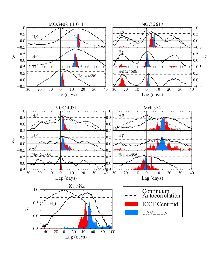
3.1 Cross-Correlation

The cross-correlation procedure derives a lag from the centroid of the interpolated cross-correlation function (ICCF, Gaskell & Peterson 1987), as implemented by Peterson et al. (2004). For a given time delay, we shift the abscissas of the first light curve, linearly interpolate the second light curve to the new time coordinates, and calculate the correlation coefficient $r_{cc}$ between all overlapping data points. We then repeat this calculation but shift the second light curve by the negative of the given time delay and interpolate the first light curve. The two values of $r_{cc}$ are averaged together, and the ICCF is evaluated by repeating this procedure on a grid of time delays spaced by 0.1 days. All ICCFs are measured relative to the 5100 Å continuum light curve (inter-calibrated with the broad-band measurements). For each line light curve, the maximum value $r_{\rm max}$ of the ICCF is given in Table 4. The lag is estimated with the ICCF centroid, defined as $\tau_{\rm cent}=\int\tau r_{cc}(\tau)\,d\tau/\int r_{cc}(\tau)\,d\tau$ for values of $r_{cc}\geq 0.8r_{\rm max}$.

We estimate the uncertainty on $\tau_{\rm cent}$ using the flux randomization/random subset sampling (FR/RSS) method of Peterson et al. (2004). This technique generates perturbed light curves by randomly selecting (with replacement) a subset of the data from both light curves and adjusting the fluxes by a Gaussian deviate scaled to the measurement uncertainties. The lag $\tau_{\rm cent}$ is calculated for $10^{3}$ perturbations of the data, and its uncertainty is estimated from the central 68% confidence interval of the resulting distribution. The ICCF and centroid distributions are shown in Figure 8 for all objects and line light curves, and Table 15 gives the median values and central 68% confidence intervals of these distributions. For completeness, we also report in Table 15 the lag $\tau_{\rm peak}$ that corresponds to $r_{\rm max}$. Note that these lags have been corrected to the rest frame of the source. For 3C 382, we do not find meaningful centroids in the ICCFs of the H$\gamma$ and Heii $\lambda 4686$ light curves. This is because of the width of the autocorrelation function of the continuum and its poor correlation with the line light curves. We therefore do not include these lines for the rest of the ICCF analysis.

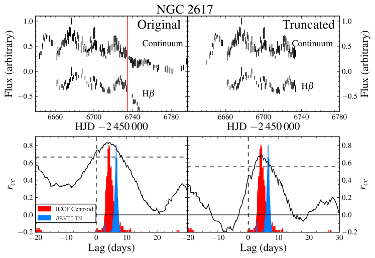
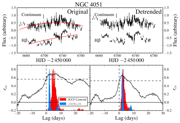
Long-term trends in the light curves can bias the resulting ICCF due to red-noise leakage (Welsh, 1999). We therefore experimented with detrending the light curves and/or restricting the baseline over which to calculate the ICCF. For MCG+08-11-011 these experiments had no effect, while for Mrk 374 and 3C 382 they eliminated any lag signal in the data. For NGC 2617, we found that restricting the data to 6 620 $<$ HJD $-$ 2 450 000 $<$ 6 730 improved the ICCF by narrowing the central peak, as shown in the top four panels of Figure 9. However, this restriction changed the ICCF centroid by only 0.01 days, a negligible amount. For NGC 2617, the peaks in the H$\gamma$ and Heii $\lambda 4686$ ICCFs at $\pm 25$ days are also obvious aliases, so we only report the lag based on the peak near 0 days. For NGC 4051, we found that detrending the continuum and line light curves with a second-order polynomial improves the ICCF, as shown in the bottom four panels of Figure 9. The long-term continuum trend is very weak, but there is a strong positive trend in the line light curves that is dominated by the linear term. Subtracting this linear trend decreases the median of the centroid distribution from 4.92 days to 2.56 days, a change of 1.5$\sigma$. We adopt the smaller lag because of the quality of the detrended ICCF, and our Bayesian method (described below) finds a lag consistent with this smaller value.

3.2 JAVELIN

We also investigated the line lags using a Bayesian approach, as implemented by the JAVELIN software (Zu et al., 2011). JAVELIN explicitly models the reverberating light curves and corresponding transfer functions so as to find a posterior probability distribution of lags. We have already discussed JAVELIN’s assumption that light curves are reasonably characterized by a DRW (§2.5.2). JAVELIN also assumes that the transfer function is a simple top-hat that can be parameterized by a width, an amplitude, and a mean time delay. This assumption is not very restrictive, since it is difficult to distinguish among transfer functions in the presence of noise (Rybicki & Kleyna, 1994; Zu et al., 2011) and a top-hat is broadly consistent with expectations for physically-plausible BLR geometries (e.g., disks or spherical shells).

We ran JAVELIN models for each line using the 5100 Å continuum as the driving light curve, and we used internal JAVELIN routines to remove any linear trends from the light curves during the fit. The damping time scale (a parameter of the DRW model) for most AGN is several hundred days or longer (Kelly et al., 2009; MacLeod et al., 2010), and our light curves are not long enough to meaningfully constrain this parameter. We therefore (arbitrarily) fixed the damping time scale to 200 days. We also tested several different damping time scales (from a few days to 500 days), and found that the choice of 200 days does not affect the best-fit lags—an exact estimate of the damping time scale is not necessary to reasonably interpolate the light curves (Kozłowski, 2016b). Table 15 gives the median and 68% confidence interval of the posterior lag distributions, denoted as $\tau_{\tt JAV}$. We also employed models that fit all light curves from a single object simultaneously, which maximizes the available information. These results are given in Table 15 as $\tau_{\rm multi}$. Posterior distributions of $\tau_{\rm multi}$ are shown by the blue histograms in Figure 8. For the H$\gamma$ and Heii $\lambda 4686$ light curves from 3C 382, we were again unable to constrain any lag signal, and we drop these light curves from the rest of this analysis.

3.3 Results

We generally find consistent results between the ICCF method and JAVELIN models. The largest discrepancies are the H$\beta$ lags for NGC 2617 ($\Delta\tau=1.6\sigma$) and 3C 382 ($\Delta\tau=2.0\sigma$), but these differences are not statistically significant. In NGC 2617, where the ICCF method detects a lag consistent with zero in the H$\gamma$ or Heii $\lambda 4686$ light curves, JAVELIN finds a lag at reasonably high confidence: the percentiles for $\tau_{\rm multi}=0$ in the posterior lag distributions of H$\gamma$ and Heii $\lambda 4686$ are 8.3% and 1.1%, which are 1.4$\sigma$ and 2.3$\sigma$ detections for Gaussian probability distributions, respectively. For Mrk 374, an H$\gamma$ lag is detected at high significance using JAVELIN (we do not claim a lag detection for Heii $\lambda 4686$ in this object, since the $\tau_{\rm multi}=0$ percentile is 20%, only $0.2\sigma$ for a Gaussian probability distribution). The detection of these lags represents a significant advantage of the JAVELIN technique over traditional cross-correlation methods. We adopt the $\tau_{\rm multi}$ as our final lag measurements, since the multi-line global fits provide well-constrained lags, properly treat covariances between the lags from different light curves, and utilize the maximum amount of information available in the data.

The analysis of NGC 4051 is especially difficult because the light curves exhibit low-amplitude variations. The lags in this object are also expected to be small, based on the AGN luminosity (Bentz et al., 2013) and a previous well-sampled RM experiment (Denney et al., 2009b). For H$\beta$, JAVELIN finds a definite lag near 2 days, consistent with the detrended ICCF approach. For H$\gamma$, the ICCF method finds a lag consistent with zero, while the single-line JAVELIN fit finds a lag of $4.87\pm 0.18$ days and the multi-line fit finds a lag of $2.40\pm 0.80$ days (rest frame). The single-line fit results in a complicated multi-modal posterior distribution with smaller peaks at 15 and 25 days that are caused by aliasing. For example, the 25-day lag is probably caused by aligning the H$\gamma$ maximum near 6745 days with the local maximum in the continuum light curve at 6720 days (Figure 4). However, the multi-line fit shows a strong, dominant peak for H$\gamma$ at $2.40$ days (rest frame). A probable explanation is that the H$\beta$ light curve matches the overall shape of H$\gamma$, but has stronger features against which to estimate a continuum lag—fitting both light curves simultaneously can therefore establish an H$\gamma$ lag with higher confidence. The problem with the H$\gamma$ light curve appears in a more serious form in the Heii $\lambda 4686$ light curve, and JAVELIN finds a lag consistent with zero for this line.

Figure 8: Lags for all emission lines in all objects. The solid lines show the ICCFs and the dashed lines show the autocorrelation function of the continuum. The red histograms show the ICCF centroid distributions for $\tau_{\rm cent}$, and the blue histograms show the posterior JAVELIN lag distributions for $\tau_{\rm multi}$. The histograms are normalized by dividing by their maximum values. The horizontal dashed lines show $0.8r_{\rm max}$, used to calculate $\tau_{\rm cent}$.

Figure 9: Comparison of two CCF analyses of the H$\beta$ light curves for NGC 2617 and NGC 4051. NGC 2617 is shown in the top four panels and NGC 4051 is shown in the bottom four. Color coding of the histograms is the same as Figure 8. The left columns show the original light curves, the right columns show the modified light curves. In the case of NGC 2617, truncating the light curves at HJD$-2\,450\,000=6\,735$ days (vertical red line, top left) helps concentrate the ICCF peak. For NGC 4051, subtracting a second-order polynomial fit to the data removes the effect of long-term secular trends (red lines, bottom-middle left panel). As a reminder, the JAVELIN fits include linear detrending, so the blue histograms are identical on the left and right sides. The same procedures were applied to all emission line light curves in these objects.

4 Linewidths and $M_{\rm BH}$ Calculations

After determining the characteristic size of the BLR from the mean time delay, the next step is to calculate the characteristic line-of-sight velocity of the BLR gas, from which we can derive SMBH masses. The BLR velocity is estimated from the width of emission lines in the MDM spectra. However, it is important to use the linewidth of the variable component of the profile, since we measure the BLR radius from the variable line flux. For example, the variable profile of 3C 382 is radically different (and much broader) than the time-averaged profile in the mean spectrum (Figure 5). We therefore measure and report in Table 16 linewidths both in the mean spectrum $\hat{F}(\lambda)$, and in the rms spectrum $\sigma_{\rm var}(\lambda)$, but we use the latter for mass determinations.

There are two common choices for linewidth measurements: the full-width at half-maximum (FWHM) and the line dispersion $\sigma_{L}$ (the rms width of the line profile). There are advantages and disadvantages associated with both approaches—while the FWHM is simpler to measure, there are ambiguities for noisy or complicated line profiles such as the double-peaked H$\beta$ profiles in MCG+08-11-011, NGC 2617, and 3C 382. On the other hand, although $\sigma_{L}$ is well-defined for arbitrary line profiles, it depends more sensitively on continuum subtraction and blending in the line wings (Denney et al., 2016; Mejía-Restrepo et al., 2016). Peterson et al. (2004) find that velocities estimated with $\sigma_{L}$ produce a tighter virial relation, and Denney et al. (2013) find that the masses determined from UV and optical lines agree better using $\sigma_{\rm L}$. We therefore adopt $\sigma_{L}$ as a measure of the BLR velocity in this study. For completeness, we also give the FWHM in Table 16.

Linewidth uncertainties are estimated using a bootstrapping method. For $10^{3}$ iterations on each object with $N$ nightly spectra, we randomly select $N$ observations with replacement, recompute the mean and rms spectrum, and remeasure the linewidths in the rms spectrum. The central 68% confidence interval of the resulting distributions are adopted as the formal uncertainty of the linewidth. This approach can only account for statistical uncertainties in the linewidths, which therefore represent lower limits on the uncertainties. There are additional systematic errors from the choice of wavelength windows that define the line profiles (Tables 2 and 3), as well as blending of the broad-line wings. The choice of wavelength windows and continuum subtraction is problematic for weak lines, lines with low variability, and lines with unusual profiles. In particular, our estimates for the Heii $\lambda 4686$ line in NGC 2617, NGC 4051, 3C 382, and all lines in Mrk 374 are certainly affected. Furthermore, the blue wing of H$\beta$ and the red wing of Heii $\lambda 4686$ overlap in MCG+08-11-011 and NGC 2617, and it is likely that the Heii $\lambda 4686$ velocity is severely underestimated (the effect on H$\beta$ is probably smaller, though it may not be negligible). Spectral decompositions may help with these problems in future analyses; for now, we note that the linewidth uncertainties are underestimated in these cases, and we provide a treatment for this issue below.

We correct the linewidth measurements for the instrument resolution by subtracting the rms width of the spectrograph’s line-spread-function (LSF) in quadrature from the observed value of $\sigma_{L}$. Previous studies have found that the width of the LSF for the MDM spectrograph is near 3.2 or 3.4 Å (FWHM 7.6–7.9 Å, Denney et al. 2010; Grier et al. 2012). Based on comparisons with high spectral resolution observations, where the LSF width is negligible, we find a LSF width of 2.97 Å (FWHM $=6.99\,\AA$). This value was determined using the catalog of high-resolution [Oiii] $\lambda 5007$ measurements from Whittle (1992), which contains intrinsic [Oiii] $\lambda 5007$ linewidths for MCG+0-11-011 and NGC 4051. The [Oiii] $\lambda 5007$ line of NGC 4051 is undersampled in the MDM spectra (the intrinsic FWHM is 190 km s^-1, or 3.16 Å in the observed frame), and does not give a reliable estimate the instrumental broadening. However, the intrinsic [Oiii] $\lambda 5007$ FWHM in MCG+08-11-011 is 605 km s^-1, or 10.52 Å in the observed frame, which is well resolved. The observed FWHM in the MCG+08-11-011 reference spectrum (before smoothing, see §2.2.2 and below) is 12.63 Å, which implies that the FWHM of the LSF is 6.99 Å (a rms width of 2.97 Å). This value is close to but slightly smaller than previous estimates. The MDM LSF may not be perfectly stable in time, so we adopt 2.97 Å as the rms width of the instrumental broadening in our observations.

An additional correction must be applied because we smooth our reference spectra to approximately match the nights with the worst spectroscopic resolution (see §2.2.2). The kernel widths for this smoothing procedure were 1.4 Å for MCG+08-11-011, 1.5 Å for NGC 2617, 1.8 Å for NGC 4051, 1.7 Å for 3C 382, and 1.9 Å for Mrk 374 (the FWHM values are a factor of 2.35 larger). We also subtract these values in quadrature from the observed line dispersion. The final rest-frame linewidths and their uncertainties are given in Table 16.

Table 16: Rest-frame Velocity Linewidth Measurements

		RMS Spectrum		Mean Spectrum
Object	Line	$\sigma_{\rm L}$	FWHM	$\sigma_{\rm L}$	FWHM
		(km s-1)	(km s-1)	(km s-1)	(km s-1)
(1)	(2)	(3)	(4)	(5)	(6)
MCG+08-11-011	H$\beta$	$1466_{-174}^{+102}$	$4475_{-356}^{+192}$	$1681_{-02}^{+02}$	$1159_{-0007}^{+0008}$
	H$\gamma$	$1604_{-082}^{+083}$	$3916_{-716}^{+616}$	$1175_{-07}^{+07}$	$1978_{-0019}^{+0026}$
	Heii$\lambda$4686	$2453_{-130}^{+125}$	$6617_{-776}^{+993}$	$2893_{-37}^{+42}$	$2517_{-1020}^{+1814}$
NGC 2617	H$\beta$	$2424_{-086}^{+091}$	$6489_{-162}^{+213}$	$2709_{-006}^{+006}$	$5303_{-46}^{+49}$
	H$\gamma$	$3084_{-090}^{+086}$	$7674_{-472}^{+423}$	$2385_{-034}^{+033}$	$4101_{-29}^{+26}$
	Heii$\lambda$4686	$2020_{-572}^{+329}$	$6788_{-855}^{+984}$	$3113_{-218}^{+147}$	$7150_{-33}^{+35}$
NGC 4051	H$\beta$	$493_{-36}^{+34}$	$941_{-019}^{+017}$	$470_{-2}^{+2}$	$765_{-03}^{+03}$
	H$\gamma$	$641_{-59}^{+55}$	$1098_{-034}^{+031}$	$942_{-4}^{+4}$	$1676_{-05}^{+06}$
	Heii$\lambda$4686	$1689_{-38}^{+36}$	$3885_{-218}^{+299}$	$1898_{-3}^{+4}$	$4598_{-11}^{+10}$
3C382	H$\beta$	$4552_{-0163}^{+0214}$	$11549_{-0667}^{+1292}$	$3227_{-07}^{+07}$	$3619_{-050}^{+282}$
	H$\gamma$	$5083_{-1942}^{+1114}$	$10706_{-1294}^{+1050}$	$2845_{-53}^{+55}$	$3483_{-022}^{+022}$
	Heii$\lambda$4686	$2073_{-0352}^{+0170}$	$4374_{-0602}^{+1257}$	$1789_{-28}^{+27}$	$5186_{-075}^{+247}$
Mrk 374	H$\beta$	$1329_{-429}^{+308}$	$3094_{-0619}^{+0488}$	$1490_{-04}^{+04}$	$3250_{-18}^{+19}$
	H$\gamma$	$1163_{-364}^{+215}$	$2311_{-0294}^{+0814}$	$1148_{-05}^{+05}$	$3648_{-18}^{+18}$
	Heii$\lambda$4686	$1997_{-223}^{+158}$	$4172_{-1083}^{+1106}$	$1554_{-70}^{+58}$	$4140_{-64}^{+64}$

Note. — Column 3 and Column 4 give the rms line width and FWHM in the rms spectrum. Column 5 and Column 6 give the same but in the mean spectrum. All values are corrected for instrumental broadening and the smoothing in §2.2.2 (see §4), and are reported in the rest-frame. The uncertainties only represent the statistical errors—blending, continuum interpolation, and the choice of wavelength windows introduce additional systematic uncertainties (especially for Heii $\lambda 4686$).

We measure the SMBH masses as

$$M_{\rm BH}=\langle f\rangle\frac{\sigma_{L}^{2}c\tau_{\rm multi}}{G}$$ (9)

where $c$ is the speed of light, $G$ is the gravitational constant, and $\langle f\rangle$ is the virial factor. The virial factor accounts for the unknown geometry and dynamics of the BLR, and is determined by calibrating a sample of RM AGN to the $M_{\rm BH}$-$\sigma_{*}$ relation (e.g., Onken et al. 2004; Park et al. 2012a; Grier et al. 2013a). We use the most recent calibration by Woo et al. (2015) of $\langle f\rangle=4.47\pm 1.25$ with a scatter of $0.43\pm 0.03$ dex (a factor of 2.7). Finally, it is convenient to define the virial product, $\sigma_{L}^{2}c\tau/G$, which is an observed quantity that is independent of the mass calibration.

We calculate the statistical uncertainties on the virial products through standard error propagation. As discussed above, there are significant systematic uncertainties on both the linewidths and the lags, which probably dominate the final error budget (see also §2.4). We estimate the systematic uncertainty using repeat RM measurements gathered from the literature. There are 17 H$\beta$-based measurements of the virial product in NGC 5548 over the last 30 years (see Bentz & Katz 2015). The (log) standard deviation of these measurements is 0.16 dex, while the mean statistical uncertainty is 0.10 dex. Taking $\sigma_{\rm sys}^{2}=\sigma_{\rm rms}^{2}-\sigma_{\rm stat}^{2}$, we estimate a systematic uncertainty floor of 0.13 dex. Experimentation with alternative line windows, continuum interpolations, and detrending procedures suggests that this value (a factor of about $1.3$) captures most of the variation in the virial products of our sample. We therefore adopt 0.13 dex as our estimate of the systematic uncertainty on each virial product, and add this value in quadrature to the statistical uncertainties for the virial products. For our final mass estimates, we also add in quadrature the the uncertainty in the mean value of $\langle f\rangle$ ($\sim\!0.12$ dex) and its intrinsic scatter (0.43 dex). The virial products, final masses, and total uncertainties are given in Table 17.

We discuss the consistency of virial products for the same object derived from different emission lines in §5.2, and we comment on the H$\beta$-derived masses of individual objects below.

Table 17: Black Hole Masses

Object	Line	$\tau$	$\sigma_{L}$	$\log\left(c\tau\sigma^{2}_{V}/G\right)$	$\log M_{\rm BH}$
		(days)	(km s-1)	[M⊙]	[M⊙]
(1)	(2)	(3)	(4)	(5)	(6)
MCG+08-11-011	H$\beta$	$14.98^{+0.34}_{-0.28}$	$1466^{+102}_{-174}$	$6.80\pm 0.15$	$7.45\pm 0.47$
	H$\gamma$	$12.38^{+0.46}_{-0.49}$	$1604^{+83}_{-82}$	$6.79\pm 0.14$	$7.44\pm 0.47$
	Heii$\lambda$4686	$1.21^{+0.29}_{-0.33}$	$2453^{+125}_{-130}$	$6.20\pm 0.18$	$6.80\pm 0.48$
NGC 2617	H$\beta$	$6.38^{+0.44}_{-0.50}$	$2424^{+91}_{-86}$	$6.86\pm 0.14$	$7.51\pm 0.47$
	H$\gamma$	$0.81^{+0.59}_{-0.61}$	$3084^{+86}_{-90}$	$6.17\pm 0.44$	$6.82\pm 0.63$
	Heii$\lambda$4686	$1.75^{+0.34}_{-0.38}$	$2020^{+329}_{-572}$	$6.14\pm 0.26$	$6.79\pm 0.52$
NGC 4051	H$\beta$	$2.24^{+0.39}_{-0.28}$	$493^{+34}_{-36}$	$5.02\pm 0.16$	$5.67\pm 0.47$
	H$\gamma$	$2.40^{+0.86}_{-0.73}$	$641^{+55}_{-59}$	$5.28\pm 0.21$	$5.93\pm 0.50$
3C382	H$\beta$	$52.07^{+3.18}_{-9.46}$	$4552^{+214}_{-163}$	$8.33\pm 0.14$	$8.98\pm 0.47$
Mrk 374	H$\beta$	$13.73^{+1.06}_{-1.02}$	$1329^{+308}_{-429}$	$6.67\pm 0.31$	$7.32\pm 0.54$
	H$\gamma$	$13.37^{+2.11}_{-2.08}$	$1163^{+215}_{-364}$	$6.55\pm 0.28$	$7.20\pm 0.53$

Note. — Column 3 gives the adopted lag and its statistical uncertainty, $\tau_{\rm multi}$, from Table 15. Column 4 gives the rms linewidth $\sigma_{\rm L}$ from Table 16 of the line profile in the rms residual spectrum and its statistical uncertainty (see §2.4 and §4), corrected to the rest-frame. Column 5 gives the virial product, which is independent of any calibration to the $M_{\rm BH}$–$\sigma_{*}$ relation. Column 6 gives the SMBH mass using the $M_{\rm BH}$–$\sigma_{*}$ calibration from Woo et al. (2015) with$f=4.47\pm 1.25$.

1. MCG+08-11-011 is our most variable object. The black hole mass estimate is $\sim\!2.8\times 10^{7}\,{\rm M_{\odot}}$, and the uncertainty is dominated by uncertainty in the virial factor $f$. Bianchi et al. (2010) found evidence for a relativistically broadened Fe K$\alpha$ line in the X-ray spectrum of this object, but the available mass estimates at that time were uncertain by an order of magnitude (10⁷–10⁸ M_⊙). The results presented here may help measure the spin of the black hole in future studies.

2. The mass reported here for NGC 2617 of $\sim\!3.2\times 10^{7}\,{\rm M_{\odot}}$ is in good agreement with the single-epoch mass estimated by Shappee et al. (2014) of $(4\pm 1)\times 10^{7}\,{\rm M_{\odot}}$, also using the H$\beta$ emission-line. NGC 2617 is the second “changing look” AGN with a direct RM mass measurement. The other object is Mrk 590, which was observed to change from a Seyfert 1.5 to 1.0 to 1.9 over several decades (Denney et al., 2014), and has a RM mass of $\sim\!5\times 10^{7}\,{\rm M_{\odot}}$ (Peterson et al., 2004). In terms of their black hole masses, there is nothing extraordinary about either NGC 2617 or Mrk 590. Our luminosity-independent RM mass also allows us to estimate a more robust Eddington ratio ($\dot{m}_{\rm Edd}=L_{\rm Bol}/L_{\rm Edd}$) than from the single-epoch mass. Assuming a bolometric correction of 10 for the 5100 Å continuum luminosity, we find that $\dot{m}_{\rm Edd}=0.01$, after correcting for host-galaxy starlight (see §5.1). This value is somewhat low, though not atypical, for Seyfert 1 galaxies.

3. For NGC 4051, our measurement of the H$\beta$ lag ($2.24\pm 0.33$ days) is in good agreement with the estimate of $1.87\pm 0.52$ days by Denney et al. (2009b). The measurement is challenging because of the low-amplitude continuum variations, variable host-galaxy contamination from aperture effects (Peterson et al., 1995), and a secular trend in the line light curve.

   Our estimate of the virial product $\sim\!1.1\times 10^{5}$ M_⊙ is also consistent at the 2$\sigma$ level with the estimate of $(3.0\pm 1.0)\times 10^{5}$ M_⊙ from Denney et al. (2010). The difference is primarily due to a decrease in the linewidth by about 400 ${\rm km\ s^{-1}}$ compared to the 2007 campaign. The line and continuum wavelength window definitions are somewhat different between the 2014 and 2007 campaigns, and we found that using the wavelength windows from Tables 2 and 3 for the rms spectrum from 2007 reduces the difference to only $\sim\!100{\rm\ km\ s^{-1}}$ (i.e., $\sigma_{\rm L}$ was about 20% larger in 2007 than in 2014). If we use the wavelength regions from Denney et al. (2010), the measurement from 2014 increases by $\sim\!120{\rm\ km\ s^{-1}}$. This suggests that the virial product is somewhat smaller than that reported by Denney et al. (2010), but the mild 2$\sigma$ discrepancy indicates that the systematic uncertainties are comparable to the formal uncertainties. The remaining 100–300 ${\rm\ km\ s^{-1}}$ difference is physical—comparing the rms line profiles between the two campaigns, we found that the core of the H$\beta$ line is much more variable in 2014 than it was in 2007, weighting $\sigma_{\rm L}$ to smaller values. The lag has only increased by 0.26 days (19%), so the virial product shows a net decrease. This might indicate a change in the geometry and/or dynamics of the BLR. The dynamical time is of order only two or three years at two light days from a $10^{6}$ M_⊙ black hole, so such a change cannot be ruled out a priori. A comparison of the velocity resolved reverberation signals between 2007 and 2014 is therefore especially interesting.

   Our SMBH mass estimate of $\sim\!4.7\times 10^{5}$ ${\rm M_{\odot}}$ for NGC 4051 is at the very low end of the SMBH scale, and there are only two other RM masses below $10^{6}$ $\rm{M_{\odot}}$: NGC 4395 (Peterson et al., 2005; Edri et al., 2012) and UGC 06728 (Bentz et al., 2016).

4. In 3C 382 the black hole mass is about $9.6\times 10^{8}$ ${\rm M_{\odot}}$, and a large source of uncertainty is the H$\beta$ lag. The $\sim$ 52 day lag is driven by the gentle inflection in the line light curve observed near the middle of the spectroscopic campaign, which was also observed in the imaging data about one month before the MDM observations began. The uncertainties on the H$\beta$ line lag are therefore quite large. By RM standards, 3C 382 is also at a moderate redshift ($z\sim 0.06$) and faint (V $\sim\!15.4$), putting it near the limit of feasibility for monitoring campaigns with a 1m-class telescope.

   Several estimates of the BLR orientation exist for this object. Emission from the radio lobes in 3C 382 dominates over that of the core, indicating that the system is viewed more edge on (Wills & Browne 1986 give the core-to-lobe ratio as $\sim\!0.1$). However, Eracleous et al. (1995) find an inclination of 45^∘ from dynamical modeling of the double-peaked broad H$\alpha$ line and show that this estimate is consistent with the radio properties. Velocity-delay maps and dynamical modeling of this object would be an interesting test of this inclination measurement. Unfortunately, the width of the continuum autocorrelation function and the low S/N of the line light curves are poorly suited for these experiments. On the other hand, a moderately inclined disk is broadly consistent with the double-peaked rms H$\beta$ and H$\gamma$ line profiles, and velocity-binned mean time delays may still provide interesting constraints on the BLR structure.

5. Mrk 374 is our least variable source. Although the H$\beta$ lag is detected at a statistically significant level, the uncertainty on the ICCF centroid is somewhat larger than for the other objects ($\sim\!33\%$). The mass is $\sim\!2.09\times 10^{7}$ ${\rm M_{\odot}}$, and the dominant uncertainty is from the linewidth measurement—it is clear from Figure 6 that the variability of the lines is very small and that there is some ambiguity in where the line profile begins and ends. At a redshift of $\sim\!0.04$, Mrk 374 is one of our fainter sources (V$=15.0$ mag), and, similar to 3C 382, it is near the practical limits of a monitoring campaign lead by a 1m-class telescope.

5 Discussion

5.1 Radius-Luminosity Relation

Figure 10: Radius–luminosity relation for the targets of this study, compared to the relation from Bentz et al. (2013). Luminosities are estimated from the mean of the continuum light curves corrected for Galactic extinction. The solid black line shows the best-fit relation measured by Bentz et al. (2013), and the dashed black lines show the dispersion around the best fit. Open circles show the luminosities corrected for host-galaxy starlight, which results in excellent agreement with the relation from Bentz et al. (2013).

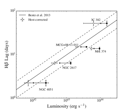
Figure 10 shows the H$\beta$ lags of our five objects as a function of luminosity, the so-called radius-luminosity ($R$–$L$) relation (Kaspi et al. 2000, 2005; Bentz et al. 2009, 2013). To estimate the luminosities, we first take the mean of the 5100 Å light curve and correct for Galactic extinction using the extinction map of Schlafly & Finkbeiner (2011) and a Cardelli, Clayton, & Mathis (1989) extinction law with $R_{V}=3.1$. We then convert the flux to luminosity using the luminosity distances in Table 1. In the case of NGC 4051, which has a large peculiar velocity relative to the Hubble flow ($z\sim 0.002$), we use a Tully-Fischer distance of 17.1 Mpc (Tully et al., 2008). This distance is uncertain by about 20%, and improving this measurement is an important step to investigate any discrepancies of this object from the $R$–$L$ relation and to estimate its true Eddington ratio. For these purposes, an HST program has recently been approved to obtain a Cepheid distance to NGC 4051 (HST GO-14697; PI Peterson).

The final values of $\lambda L_{5100\text{\AA}}$ are reported in Table 1, along with the adopted Galactic values of $E(B-V)$. We find that our objects all lie close to, but slightly below (except for 3C 382), the $R$–$L$ relation. The major systematic uncertainties are internal extinction in the AGN and host-galaxy contamination. Internal extinction may move the points farther from the $R$–$L$ relation, but this effect is expected to be small. On the other hand, host-galaxy contamination can be very significant, especially for low-luminosity objects.

In order to correct for host contamination, we model high-resolution images of the targets and isolate the host-galaxy flux. This has previously been done for NGC 4051 (Bentz et al., 2006, 2013), and MCG+08-11-011, NGC 2617, and Mrk 374 were recently observed with HST for this purpose (HST GO-13816; PI Bentz). We also retrieved archival optical WFPC2 imaging of 3C 382 (HST GO-6967, PI Sparks), but the data are not ideal for image decompositions and we discuss the host-galaxy flux estimate for this object separately. A more detailed analysis of the HST GO-13816 data and image decompositions will be presented in future work (Bentz et al, in preparation). However, following the procedures described by Bentz et al. (2013), we made preliminary estimates of the host-galaxy contributions in the MDM aperture ($15\farcs 0\times 5\farcs 0$ aligned at position angle $0^{\circ}$). The results are given in Table 1 (uncertainties on these values are estimated at 10% and included in Figure 10). Applying this correction shows that host-contamination accounts for the entire discrepancy between the observed luminosities and the $R$–$L$ relation. The largest deviation from the $R$–$L$ relation is Mrk 374, but the offset is only slightly greater than the $1\sigma$ scatter of the relation.

3C 382 resides in a giant elliptical galaxy and there may be a significant contribution from the host’s starlight—several stellar absorption features are visible in the mean spectrum in Figure 5. In the archival HST images, the galaxy nucleus is saturated, hindering our ability to robustly remove the AGN flux and isolate the host’s starlight. The main problem is that the Sersic index of the host-galaxy is degenerate with the saturated core and tends to drift toward unreasonably high values ($n\approx 7.6$) when fitting the image in the same way as Bentz et al. (2013). Fixing the Sersic index to more typical values (between 2 and 4) leads to host fluxes in the MDM aperture between 2.2 and 2.7$\times 10^{-15}$ erg cm^-2 s^-1 Å^-1, about 77% of the observed luminosity ($\log\lambda L_{\rm host}=44.04$ to 44.12 [erg s^-1], after correcting for Galactic extinction). This estimate can be checked using the equivalent-width (EW) of the prominent Mg absorption feature at 5200 Å rest-frame (5460 Å observed-frame). In our mean spectrum, we find an EW of 2.8 Å. In typical elliptical galaxy spectra, we find the EW is about 6.7 to 7.3 Å, depending on the continuum estimation and assumptions about the host-galaxy properties. This implies that the featureless AGN continuum dilutes the absorption feature by a factor of 2.4 to 2.6, so that the host galaxy contributes approximately 40% of the observed luminosity. This rough estimate is a factor of two lower than the result from image decomposition, but the two values span the range of host-contributions from the other objects in our sample (42% to 71% of the observed luminosity, see Table 1). We therefore adopt a host correction of $(60\pm 20)$% of the observed luminosity ($\log\lambda L_{\rm 5100\text{\AA}}=43.98\pm 0.15$ [erg s^-1]), and we note that this estimate can easily be improved by obtaining unsaturated high resolution images. The host correction moves 3C 382 away from the $R$–$L$ relation, just beyond the $1\sigma$ dispersion. However, considering the large uncertainties, there does not appear to be any evidence that 3C 382 has an anomalous H$\beta$ lag for its luminosity.

5.2 Virialization of the BLR

Figure 11: Linewidth $\sigma_{\rm L}$ as a function of lag $\tau_{\rm multi}$ from Columns 3 and 4 of Table 17. The solid lines show the virial relation $\sigma_{\rm L}\propto\tau_{\rm multi}^{-1/2}$ normalized by the H$\beta$ virial product (VP_Hβ). The dashed lines show the virial relation using a weighted average of the different emission line virial products (Column 5 of Table 17). The open points for MCG+08-11-011 and NGC 2617 show the effect of adding a hypothetical 2.0 day UV–optical lag, similar to that found in NGC 5548 (see §5.2). For NGC 4051 and Mrk 374, the Heii $\lambda 4686$ lags are consistent with zero, and we show these as upper limits at 1 day. Uncertainties of 0.13 dex are assigned to both $\tau_{\rm multi}$ and $\sigma_{\rm L}$, to approximately represent the level of systematic uncertainty associated with the virial products.

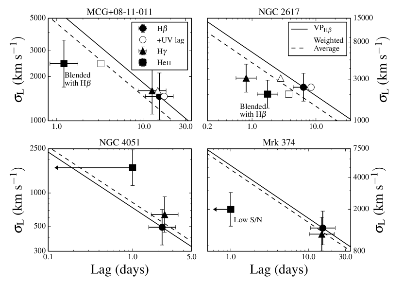
With the measurement of BLR velocity dispersions at a range of radii, it is possible to test if the BLR is virialized. Virialized dynamics predict $V(r)\propto r^{-1/2}$, where the constant of proportionality depends on the SMBH mass and BLR inclination/kinematics. If the BLR is virialized, the virial products $\sigma_{L}^{2}c\tau/G$ derived from different line species should be consistent with each other, assuming similar geometries and dynamics for the line-emitting gas.

In Table 17, the maximum differences between $\log\sigma_{L}^{2}c\tau/G$ for each object are $3.3\sigma$ in MCG+08-11-011, $2.8\sigma$ in NGC 2617, $1.2\sigma$ in NGC 4051, and $0.4\sigma$ in Mrk 374. For NGC 4051 and Mrk 374, these differences are not significant. For MCG+08-11-011 and NGC 2617, the H$\beta$ and Heii $\lambda 4686$ virial products are marginally discrepant at about 2.5–3.3$\sigma$. We show these results Figure 11, which displays the linewidths $\sigma_{\rm L}$ as a function of lag $\tau_{\rm multi}$, and the relation $\sigma_{\rm L}\propto\tau_{\rm multi}^{-1/2}$ normalized by the value for H$\beta$. In this figure, we have applied a 0.13 dex uncertainty to both the lag $\tau$ and line width $\sigma_{\rm L}$, representative of the characteristic systematic uncertainties. While the H$\gamma$ points generally agree with the H$\beta$ relation, the Heii $\lambda 4686$ points have very large offsets.

There are many systematic issues that could account for these differences. As discussed in §4, the red wing of Heii $\lambda 4686$ is blended with the blue wing of H$\beta$ in both MCG+08-11-011 and NGC 2617. The Heii $\lambda 4686$ velocity is therefore likely underestimated because we cannot follow its red wing underneath H$\beta$. The Heii $\lambda 4686$ lags are also small compared to the monitoring cadence, and the lag is only marginally detected at 2.3$\sigma$ in NGC 2617. Furthermore, the choice of line window and continuum interpolation can have a significant effect on the lag and linewidths. Finally, we must assume that the 5100 Å continuum light curve is a suitable proxy for the ionizing flux variations at extreme UV wavelengths. In NGC 5548, we found a $\sim\!2$ day lag between the far UV and optical emission (Edelson et al., 2015; Fausnaugh et al., 2016). If a similar lag exists in these objects, it would change the Heii $\lambda 4686$ virial products by a significant amount (0.3–0.4 dex), while the change in the H$\beta$ virial products would be much smaller (0.05–0.11 dex). The effect of adding a 2 day UV-optical lag to the optical-line lags is shown in Figure 11, and the additional lag would reduce the discrepancies in the virial products to 1.3$\sigma$ for MCG+08-11-011 and 2.0$\sigma$ for NGC 2617. These AGN have masses and luminosities similar to NGC 5548, so the existence of a UV-optical lag of this magnitude is very likely. Although a UV-optical lag affects the virial product and the characteristic size of the BLR, it does not affect the final mass estimate because the virial factor $\langle f\rangle$ is calibrated using the $M_{\rm BH}$–$\sigma_{*}$ relation (see Fausnaugh et al. 2016; Pei et al. 2017).

If the remaining discrepancies are real, they indicate different dynamics and geometries for the Heii $\lambda 4686$ line-emitting gas compared to that of H$\beta$. This might be plausible, since Heii $\lambda 4686$ is a high-ionization state line and may originate in very different physical conditions than the Balmer lines (for example, a disk wind). If Heii $\lambda 4686$ has different dynamics than H$\beta$, it would be necessary to calibrate a different virial factor $\langle f\rangle$ for the Heii $\lambda 4686$ line when calculating the SMBH masses. However, we cannot rule out systematic effects and it is unclear if the Heii $\lambda 4686$ discrepancies are physical. If systematic issues do account for the discrepancies, then the dynamics of the BLRs in these AGN would be consistent with virialized motion, as has been found for other AGN (Peterson et al., 2004).

The H$\beta$ light curves and line profiles have much higher S/N and very clear lags compared to both Heii $\lambda 4686$ and H$\gamma$, resulting in more reliable black hole masses. If we combine the virial products in Table 17 using an error-weighted average, the virial relation changes little, as shown in Figure 11 with the dashed lines. We therefore take the H$\beta$ masses for our standard SMBH mass estimates.

Figure 12: Responsivities of optical recombination lines relative to H$\beta$. The results for H$\gamma$ are shown in purple and those for Heii $\lambda 4686$ are shown in red. Solid lines show weighted linear-least squares fits (accounting for uncertainties in both coordinates)—the slope of the fit gives the relative responsivity, which is listed in each panel. See §5.3 for more details.

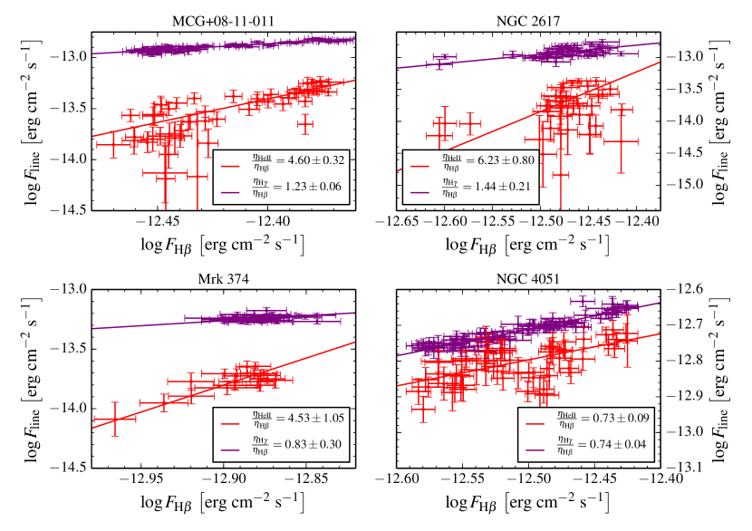
5.3 Photoionization Physics

Photoionization models make predictions about the structure of the BLR that can be tested with RM of multiple recombination lines. The locally optimally emitting cloud model (Baldwin et al., 1995) provides a natural explanation for the general similarity of AGN spectra, and predicts radial stratification of the BLR—high-ionization state lines, such as Heii $\lambda$1640/4686 and Civ $\lambda 1549$, should be primarily emitted at smaller radii than low-ionization state lines such as H$\beta$ and Mgii $\lambda 2798$. Korista & Goad (2004, hereinafter KG04) use this model to predict that the responsivity of high-order Balmer lines should be greater than that of low-order lines (in the sense that ${\rm H\gamma>H\beta>H\alpha}$). KG04 also predict that high-ionization state lines such as Heii $\lambda 4686$ should have greater responsivity than all of the Balmer lines. Radial stratification of the BLR in NGC 5548 was first observed by Clavel et al. (1991), and has since been observed in several other objects (Peterson et al. 2004; Grier et al. 2013b). In addition, the expected trends of responsivity with ionization state/species have been confirmed in 16 AGN by LAMP (Bentz et al., 2010; Barth et al., 2015).

We confirm these results for the four objects with multiple line light curves presented here. The Heii $\lambda 4686$ lags in MCG+08-11-011 and NGC 2617 are less than 2 days, while the H$\beta$ lags are 14.82 and 6.38 days, respectively, clearly indicating radial stratification. Furthermore, the fractional variability of the light curves, as measured by $F_{\rm var}$ (Table 4), is generally larger for H$\gamma$ than H$\beta$ (or comparable for NGC 4051 and Mrk 374), while $F_{\rm var}$ for Heii $\lambda 4686$ is always much greater than for the Balmer lines (although it is only slightly higher in NGC 4051). This implies that the relative line responsivities are Heii $\lambda 4686$ $\gg$ H$\gamma$ $>$ H$\beta$, in agreement with the photoionization models. We also find that the H$\gamma$ lags are slightly shorter than the H$\beta$ lags within the same object (except for NGC 4051). KG04 show that shorter lags are a natural consequence of the higher responsivity of H$\gamma$ compared to H$\beta$.

The formal definition of the responsivity of an emission line is

$$\eta_{\rm line}=\frac{\Delta\log F_{\rm line}}{\Delta\log\Phi}$$ (10)

where $F_{\rm line}$ is the line flux and $\Phi$ is the photoionizing flux (KG04). The parameter $\eta_{\rm line}$ is therefore a measure of how efficiently the BLR converts a change in the photoionizing flux into a change in line emission. The ionizing flux $\Phi$ cannot be observed directly because these photons are at far UV wavelengths ($<912$ Å). Therefore, we cannot measure $\eta_{\rm line}$ directly, but we can measure the relative responsivity $\eta_{\rm line1}/\eta_{\rm line2}=\Delta\log F_{\rm line1}/\Delta\log F_{\rm line2}$.

We present rough measurements of the relative responsivity of H$\beta$, H$\gamma$, and Heii $\lambda 4686$ in Figure 12. For each object, we first removed the lags of each line from the corresponding light curve. We then matched observed points to the nearest day between the H$\beta$ light curves and H$\gamma$ or Heii $\lambda 4686$ light curves. The ratio $\eta_{\rm line}/\eta_{\rm H\beta}$ then corresponds to the slope of a linear least-squares fit to the data in the $\log F_{\rm H\beta}$-$\log F_{\rm line}$ plane.

We find that $\eta_{\rm H\gamma}/\eta_{\rm H\beta}$ ranges from $0.74$ to $1.44$ and that $\eta_{\rm He{\sc II}}/\eta_{\rm H\beta}$ ranges between $0.73$ and $6.23$. NGC 4051, with $\eta_{\rm He{\sc II}}/\eta_{\rm H\beta}\sim 0.73$, is an outlier, probably caused by over-subtracting the continuum before integrating the line flux. For comparison, KG04 calculate $\eta_{\rm line}$ for a fiducial model of the BLR in NGC 5548, which includes an empirically motivated but ad hoc parameterization of the ionizing flux. From their Table 1, $\eta_{\rm H\gamma}/\eta_{\rm H\beta}$ ranges between 1.03 and 1.07, depending on the flux state of the AGN, while $\eta_{\rm He{\sc II}}/\eta_{\rm H\beta}$ ranges from 1.26 to 1.61. Thus, while our fits for $\eta_{\rm H\gamma}/\eta_{\rm H\beta}$ are in reasonable agreement with this fiducial model, the values of $\eta_{\rm He{\sc II}}/\eta_{\rm H\beta}$ are much larger than the model’s prediction. The spread of $\eta_{\rm line}/\eta_{\rm H\beta}$ in our fits is also fairly large, which may indicate a diversity of photoionization conditions in the BLRs of different objects (perhaps due to harder or softer ionizing fluxes than assumed for NGC 5548).

Our estimates of the relative responsivities are sensitive to the total flux of the line light curves. For example, the sublinear slopes for $\eta_{\rm H\gamma}/\eta_{\rm H\beta}$ in NGC 4051 and Mrk 374 could be explained by missing variable line flux, perhaps in the wings of the line during low-flux states, or excess constant flux from the narrow emission lines or host-galaxy starlight. On the other hand, large values of $\eta_{\rm He{\sc II}}/\eta_{\rm H\beta}$ might be explained by contamination by Feii lines or misestimation of the continuum.

6 Summary and Future Prospects

We have presented the initial analysis of data from an intensive RM monitoring campaign carried out in the first half of 2014. We succeeded in measuring continuum-line lags for six targets, five of which are presented here. (For NGC 5548, see Pei et al. 2017.) Our main results are:

1. Four new SMBH masses, as well as a refined measurement for NGC 4051.

2. In addition to measuring H$\beta$ lags for all five targets, we measure H$\gamma$ lags in four objects and Heii $\lambda 4686$ lags in two objects.

3. Using the Heii $\lambda 4686$ lags (or their upper limits), we show that the BLR is radially stratified. Although the Heii $\lambda 4686$ virial products are somewhat smaller than those derived from H$\beta$, systematic effects such as blending in the line wings and the choice of continuum interpolation may account for these discrepancies. The BLRs are otherwise consistent with virialized dynamics with $V(r)\propto r^{-1/2}$.

4. We find that Heii $\lambda 4686$ is more responsive than the Balmer lines, and that H$\gamma$ is more responsive than H$\beta$, in agreement with predictions from photoionization modeling.

Many modern RM experiments are focused on measuring velocity-resolved reverberation signatures, in order to investigate the geometry and dynamics of the BLR. There are only six AGN with published velocity-delay maps (Ulrich & Horne, 1996; Bentz et al., 2010; Grier et al., 2013b) and five AGN with direct BLR dynamical models (Pancoast et al. 2014b; one AGN, Arp 151, has both). The data presented here are of exceptional quality and very well-calibrated—based on the cadence and S/N of these observations, we have an excellent prospect of recovering velocity-delay maps and dynamical models in three objects (MCG+08-11-011, NGC 2617, and NGC 4051). This will expand the sample of AGN with detailed BLR information by $\sim$30%, demonstrating the continuing importance of targeted and intensive monitoring campaigns.

References

- Alard & Lupton (1998) Alard, C., & Lupton, R. H. 1998, ApJ, 503, 325
- Antonucci (1993) Antonucci, R. 1993, ARA&A, 31, 473
- Astropy Collaboration et al. (2013) Astropy Collaboration, Robitaille, T. P., Tollerud, E. J., et al. 2013, A&A, 558, A33
- Balbus & Hawley (1998) Balbus, S. A., & Hawley, J. F. 1998, Reviews of Modern Physics, 70, 1
- Baldwin et al. (1995) Baldwin, J., Ferland, G., Korista, K., & Verner, D. 1995, ApJ, 455, L119
- Barth et al. (2015) Barth, A. J., Bennert, V. N., Canalizo, G., et al. 2015, ApJS, 217, 26
- Bentz & Katz (2015) Bentz, M. C., & Katz, S. 2015, PASP, 127, 67
- Bentz et al. (2009) Bentz, M. C., Peterson, B. M., Netzer, H., Pogge, R. W., & Vestergaard, M. 2009, ApJ, 697, 160
- Bentz et al. (2006) Bentz, M. C., Peterson, B. M., Pogge, R. W., Vestergaard, M., & Onken, C. A. 2006, ApJ, 644, 133
- Bentz et al. (2010) Bentz, M. C., Horne, K., Barth, A. J., et al. 2010, ApJ, 720, L46
- Bentz et al. (2013) Bentz, M. C., Denney, K. D., Grier, C. J., et al. 2013, ApJ, 767, 149
- Bentz et al. (2016) Bentz, M. C., Batiste, M., Seals, J., et al. 2016, ApJ, 831, 2
- Bianchi et al. (2010) Bianchi, S., de Angelis, I., Matt, G., et al. 2010, A&A, 522, A64
- Blackburne et al. (2011) Blackburne, J. A., Pooley, D., Rappaport, S., & Schechter, P. L. 2011, ApJ, 729, 34
- Blandford & McKee (1982) Blandford, R. D., & McKee, C. F. 1982, ApJ, 255, 419
- Brosch et al. (2008) Brosch, N., Polishook, D., Shporer, A., et al. 2008, Ap&SS, 314, 163
- Brown et al. (2013) Brown, T. M., Baliber, N., Bianco, F. B., et al. 2013, PASP, 125, 1031
- Bruzual & Charlot (2003) Bruzual, G., & Charlot, S. 2003, MNRAS, 344, 1000
- Burbidge (1967) Burbidge, E. M. 1967, ARA&A, 5, 399
- Cardelli et al. (1989) Cardelli, J. A., Clayton, G. C., & Mathis, J. S. 1989, ApJ, 345, 245
- Clavel et al. (1989) Clavel, J., Wamsteker, W., & Glass, I. S. 1989, ApJ, 337, 236
- Clavel et al. (1991) Clavel, J., Reichert, G. A., Alloin, D., et al. 1991, ApJ, 366, 64
- Collin-Souffrin (1987) Collin-Souffrin, S. 1987, A&A, 179, 60
- Czerny & Hryniewicz (2011) Czerny, B., & Hryniewicz, K. 2011, A&A, 525, L8
- De Rosa et al. (2015) De Rosa, G., Peterson, B. M., Ely, J., et al. 2015, ApJ, 806, 128
- Denney et al. (2009a) Denney, K. D., Peterson, B. M., Dietrich, M., Vestergaard, M., & Bentz, M. C. 2009a, ApJ, 692, 246
- Denney et al. (2013) Denney, K. D., Pogge, R. W., Assef, R. J., et al. 2013, ApJ, 775, 60
- Denney et al. (2009b) Denney, K. D., Watson, L. C., Peterson, B. M., et al. 2009b, ApJ, 702, 1353
- Denney et al. (2010) Denney, K. D., Peterson, B. M., Pogge, R. W., et al. 2010, ApJ, 721, 715
- Denney et al. (2014) Denney, K. D., De Rosa, G., Croxall, K., et al. 2014, ApJ, 796, 134
- Denney et al. (2016) Denney, K. D., Horne, K., Shen, Y., et al. 2016, ApJS, 224, 14
- Dietrich et al. (2012) Dietrich, M., Peterson, B. M., Grier, C. J., et al. 2012, ApJ, 757, 53
- Du et al. (2016) Du, P., Lu, K.-X., Hu, C., et al. 2016, ApJ, 820, 27
- Edelson et al. (2014) Edelson, R., Vaughan, S., Malkan, M., et al. 2014, ApJ, 795, 2
- Edelson et al. (2015) Edelson, R., Gelbord, J. M., Horne, K., et al. 2015, ApJ, 806, 129
- Edri et al. (2012) Edri, H., Rafter, S. E., Chelouche, D., Kaspi, S., & Behar, E. 2012, ApJ, 756, 73
- Elitzur & Netzer (2016) Elitzur, M., & Netzer, H. 2016, MNRAS, 459, 585
- Elitzur & Shlosman (2006) Elitzur, M., & Shlosman, I. 2006, ApJ, 648, L101
- Elvis (2000) Elvis, M. 2000, ApJ, 545, 63
- Eracleous et al. (1995) Eracleous, M., Livio, M., Halpern, J. P., & Storchi-Bergmann, T. 1995, ApJ, 438, 610
- Fausnaugh (2017) Fausnaugh, M. M. 2017, PASP, 129, 024007
- Fausnaugh et al. (2016) Fausnaugh, M. M., Denney, K. D., Barth, A. J., et al. 2016, ApJ, 821, 56
- Gaskell et al. (2008) Gaskell, C. M., Goosmann, R. W., & Klimek, E. S. 2008, Mem. Soc. Astron. Italiana, 79, 1090
- Gaskell & Peterson (1987) Gaskell, C. M., & Peterson, B. M. 1987, ApJS, 65, 1
- Goad et al. (2012) Goad, M. R., Korista, K. T., & Ruff, A. J. 2012, MNRAS, 426, 3086
- Goad et al. (2016) Goad, M. R., Korista, K. T., De Rosa, G., et al. 2016, ApJ, 824, 11
- Grier et al. (2012) Grier, C. J., Peterson, B. M., Pogge, R. W., et al. 2012, ApJ, 755, 60
- Grier et al. (2013a) Grier, C. J., Martini, P., Watson, L. C., et al. 2013a, ApJ, 773, 90
- Grier et al. (2013b) Grier, C. J., Peterson, B. M., Horne, K., et al. 2013b, ApJ, 764, 47
- Hartman et al. (2004) Hartman, J. D., Bakos, G., Stanek, K. Z., & Noyes, R. W. 2004, AJ, 128, 1761
- Higginbottom et al. (2014) Higginbottom, N., Proga, D., Knigge, C., et al. 2014, ApJ, 789, 19
- Horne (1994) Horne, K. 1994, in Astronomical Society of the Pacific Conference Series, Vol. 69, Reverberation Mapping of the Broad-Line Region in Active Galactic Nuclei, ed. P. M. Gondhalekar, K. Horne, & B. M. Peterson, 23
- Horne et al. (2004) Horne, K., Peterson, B. M., Collier, S. J., & Netzer, H. 2004, PASP, 116, 465
- Hunter (2007) Hunter, J. D. 2007, Computing in Science & Engineering, 9, 90
- Kasliwal et al. (2015) Kasliwal, V. P., Vogeley, M. S., & Richards, G. T. 2015, MNRAS, 451, 4328
- Kaspi et al. (2005) Kaspi, S., Maoz, D., Netzer, H., et al. 2005, ApJ, 629, 61
- Kaspi et al. (2000) Kaspi, S., Smith, P. S., Netzer, H., et al. 2000, ApJ, 533, 631
- Kelly et al. (2009) Kelly, B. C., Bechtold, J., & Siemiginowska, A. 2009, ApJ, 698, 895
- Kinney et al. (1996) Kinney, A. L., Calzetti, D., Bohlin, R. C., et al. 1996, ApJ, 467, 38
- Kishimoto et al. (2007) Kishimoto, M., Hönig, S. F., Beckert, T., & Weigelt, G. 2007, A&A, 476, 713
- Koratkar & Blaes (1999) Koratkar, A., & Blaes, O. 1999, PASP, 111, 1
- Korista & Goad (2004) Korista, K. T., & Goad, M. R. 2004, ApJ, 606, 749
- Kozłowski (2016a) Kozłowski, S. 2016a, MNRAS, 459, 2787
- Kozłowski (2016b) —. 2016b, ApJ, 826, 118
- LaMassa et al. (2015) LaMassa, S. M., Cales, S., Moran, E. C., et al. 2015, ApJ, 800, 144
- Lawrence (1991) Lawrence, A. 1991, MNRAS, 252, 586
- MacLeod et al. (2010) MacLeod, C. L., Ivezić, Ž., Kochanek, C. S., et al. 2010, ApJ, 721, 1014
- MacLeod et al. (2016) MacLeod, C. L., Ross, N. P., Lawrence, A., et al. 2016, MNRAS, 457, 389
- McHardy et al. (2016) McHardy, I. M., Connolly, S. D., Peterson, B. M., et al. 2016, Astronomische Nachrichten, 337, 500
- McLure & Dunlop (2004) McLure, R. J., & Dunlop, J. S. 2004, MNRAS, 352, 1390
- Mejía-Restrepo et al. (2016) Mejía-Restrepo, J. E., Trakhtenbrot, B., Lira, P., Netzer, H., & Capellupo, D. M. 2016, MNRAS, 460, 187
- Miller et al. (2010) Miller, L., Turner, T. J., Reeves, J. N., et al. 2010, MNRAS, 403, 196
- Mor & Netzer (2012) Mor, R., & Netzer, H. 2012, MNRAS, 420, 526
- Morgan et al. (2010) Morgan, C. W., Kochanek, C. S., Morgan, N. D., & Falco, E. E. 2010, ApJ, 712, 1129
- Mosquera et al. (2013) Mosquera, A. M., Kochanek, C. S., Chen, B., et al. 2013, ApJ, 769, 53
- Murray & Chiang (1997) Murray, N., & Chiang, J. 1997, ApJ, 474, 91
- Nenkova et al. (2008) Nenkova, M., Sirocky, M. M., Nikutta, R., Ivezić, Ž., & Elitzur, M. 2008, ApJ, 685, 160
- Netzer & Laor (1993) Netzer, H., & Laor, A. 1993, ApJ, 404, L51
- Oke (1990) Oke, J. B. 1990, AJ, 99, 1621
- Oknyanskij & Horne (2001) Oknyanskij, V. L., & Horne, K. 2001, in Astronomical Society of the Pacific Conference Series, Vol. 224, Probing the Physics of Active Galactic Nuclei, ed. B. M. Peterson, R. W. Pogge, & R. S. Polidan, 149
- Oliphant (2007) Oliphant, T. E. 2007, Computing in Science & Engineering, 9, 10
- Onken et al. (2004) Onken, C. A., Ferrarese, L., Merritt, D., et al. 2004, ApJ, 615, 645
- Osterbrock et al. (1975) Osterbrock, D. E., Koski, A. T., & Phillips, M. M. 1975, ApJ, 197, L41
- Osterbrock et al. (1976) —. 1976, ApJ, 206, 898
- Pancoast et al. (2014a) Pancoast, A., Brewer, B. J., & Treu, T. 2014a, MNRAS, 445, 3055
- Pancoast et al. (2014b) Pancoast, A., Brewer, B. J., Treu, T., et al. 2014b, MNRAS, 445, 3073
- Park et al. (2012a) Park, D., Kelly, B. C., Woo, J.-H., & Treu, T. 2012a, ApJS, 203, 6
- Park et al. (2013) Park, D., Woo, J.-H., Denney, K. D., & Shin, J. 2013, ApJ, 770, 87
- Park et al. (2012b) Park, D., Woo, J.-H., Treu, T., et al. 2012b, ApJ, 747, 30
- Pei et al. (2017) Pei, L., Fausnaugh, M. M., Barth, A. J., et al. 2017, ApJ, 837, 131
- Peterson (1993) Peterson, B. M. 1993, PASP, 105, 247
- Peterson (2014) —. 2014, Space Sci. Rev., 183, 253
- Peterson et al. (1995) Peterson, B. M., Pogge, R. W., Wanders, I., Smith, S. M., & Romanishin, W. 1995, PASP, 107, 579
- Peterson et al. (2000) Peterson, B. M., McHardy, I. M., Wilkes, B. J., et al. 2000, ApJ, 542, 161
- Peterson et al. (2004) Peterson, B. M., Ferrarese, L., Gilbert, K. M., et al. 2004, ApJ, 613, 682
- Peterson et al. (2005) Peterson, B. M., Bentz, M. C., Desroches, L.-B., et al. 2005, ApJ, 632, 799
- Proga & Kallman (2004) Proga, D., & Kallman, T. R. 2004, ApJ, 616, 688
- Proga & Kurosawa (2010) Proga, D., & Kurosawa, R. 2010, in Astronomical Society of the Pacific Conference Series, Vol. 427, Accretion and Ejection in AGN: a Global View, ed. L. Maraschi, G. Ghisellini, R. Della Ceca, & F. Tavecchio, 41
- Rodríguez-Pascual et al. (1997) Rodríguez-Pascual, P. M., Alloin, D., Clavel, J., et al. 1997, ApJS, 110, 9
- Ruan et al. (2016) Ruan, J. J., Anderson, S. F., Cales, S. L., et al. 2016, ApJ, 826, 188
- Runco et al. (2016) Runco, J. N., Cosens, M., Bennert, V. N., et al. 2016, ApJ, 821, 33
- Runnoe et al. (2016) Runnoe, J. C., Cales, S., Ruan, J. J., et al. 2016, MNRAS, 455, 1691
- Rybicki & Kleyna (1994) Rybicki, G. B., & Kleyna, J. T. 1994, in Astronomical Society of the Pacific Conference Series, Vol. 69, Reverberation Mapping of the Broad-Line Region in Active Galactic Nuclei, ed. P. M. Gondhalekar, K. Horne, & B. M. Peterson, 85
- Sakata et al. (2010) Sakata, Y., Minezaki, T., Yoshii, Y., et al. 2010, ApJ, 711, 461
- Schlafly & Finkbeiner (2011) Schlafly, E. F., & Finkbeiner, D. P. 2011, ApJ, 737, 103
- Schmidt (1963) Schmidt, M. 1963, Nature, 197, 1040
- Sergeev et al. (2005) Sergeev, S. G., Doroshenko, V. T., Golubinskiy, Y. V., Merkulova, N. I., & Sergeeva, E. A. 2005, ApJ, 622, 129
- Shapovalova et al. (2010) Shapovalova, A. I., Popović, L. Č., Burenkov, A. N., et al. 2010, A&A, 517, A42
- Shappee et al. (2014) Shappee, B. J., Prieto, J. L., Grupe, D., et al. 2014, ApJ, 788, 48
- Shemmer et al. (2003) Shemmer, O., Uttley, P., Netzer, H., & McHardy, I. M. 2003, MNRAS, 343, 1341
- Simpson (2005) Simpson, C. 2005, MNRAS, 360, 565
- Skielboe et al. (2015) Skielboe, A., Pancoast, A., Treu, T., et al. 2015, MNRAS, 454, 144
- Suganuma et al. (2006) Suganuma, M., Yoshii, Y., Kobayashi, Y., et al. 2006, ApJ, 639, 46
- Tody (1986) Tody, D. 1986, in Proc. SPIE, Vol. 627, Instrumentation in astronomy VI, ed. D. L. Crawford, 733
- Trakhtenbrot & Netzer (2012) Trakhtenbrot, B., & Netzer, H. 2012, MNRAS, 427, 3081
- Tully et al. (2008) Tully, R. B., Shaya, E. J., Karachentsev, I. D., et al. 2008, ApJ, 676, 184
- Turner et al. (2017) Turner, T. J., Miller, L., Reeves, J. N., & Braito, V. 2017, MNRAS, 467, 3924
- Ulrich & Horne (1996) Ulrich, M.-H., & Horne, K. 1996, MNRAS, 283, 748
- Valenti et al. (2015) Valenti, S., Sand, D. J., Barth, A. J., et al. 2015, ApJ, 813, L36
- van der Walt et al. (2011) van der Walt, S., Colbert, S. C., & Varoquaux, G. 2011, Computing in Science & Engineering, 13, 22
- van Dokkum (2001) van Dokkum, P. G. 2001, PASP, 113, 1420
- van Groningen & Wanders (1992) van Groningen, E., & Wanders, I. 1992, PASP, 104, 700
- Vaughan et al. (2003) Vaughan, S., Edelson, R., Warwick, R. S., & Uttley, P. 2003, MNRAS, 345, 1271
- Vazquez et al. (2015) Vazquez, B., Galianni, P., Richmond, M., et al. 2015, ApJ, 801, 127
- Vestergaard & Peterson (2006) Vestergaard, M., & Peterson, B. M. 2006, ApJ, 641, 689
- Wandel et al. (1999) Wandel, A., Peterson, B. M., & Malkan, M. A. 1999, ApJ, 526, 579
- Wanders et al. (1997) Wanders, I., Peterson, B. M., Alloin, D., et al. 1997, ApJS, 113, 69
- Weedman (1977) Weedman, D. W. 1977, ARA&A, 15, 69
- Welsh (1999) Welsh, W. F. 1999, PASP, 111, 1347
- Whittle (1992) Whittle, M. 1992, ApJS, 79, 49
- Wilhite et al. (2005) Wilhite, B. C., Vanden Berk, D. E., Kron, R. G., et al. 2005, ApJ, 633, 638
- Wills & Browne (1986) Wills, B. J., & Browne, I. W. A. 1986, ApJ, 302, 56
- Woo et al. (2015) Woo, J.-H., Yoon, Y., Park, S., Park, D., & Kim, S. C. 2015, ApJ, 801, 38
- Yuan & Narayan (2014) Yuan, F., & Narayan, R. 2014, ARA&A, 52, 529
- Zu et al. (2013) Zu, Y., Kochanek, C. S., Kozłowski, S., & Udalski, A. 2013, ApJ, 765, 106
- Zu et al. (2011) Zu, Y., Kochanek, C. S., & Peterson, B. M. 2011, ApJ, 735, 80