Separating Double-Beta Decay Events from Solar Neutrino Interactions in a Kiloton-Scale Liquid Scintillator Detector By Fast Timing

Abstract

We present a technique for separating nuclear double beta decay ($\beta\beta$-decay) events from background neutrino interactions due to ⁸B decays in the sun. This background becomes dominant in a kiloton-scale liquid-scintillator detector deep underground and is usually considered as irreducible due to an overlap in deposited energy with the signal. However, electrons from 0$\nu\beta\beta$-decay often exceed the Cherenkov threshold in liquid scintillator, producing photons that are prompt and correlated in direction with the initial electron direction. The use of large-area fast photodetectors allows some separation of these prompt photons from delayed isotropic scintillation light and, thus, the possibility of reconstructing the event topology. Using a simulation of a 6.5 m radius liquid scintillator detector with 100 ps resolution photodetectors, we show that a spherical harmonics analysis of early-arrival light can discriminate between 0$\nu\beta\beta$-decay signal and ⁸B  solar neutrino background events on a statistical basis. Good separation will require the development of a slow scintillator with a 5 nsec risetime.

1 Introduction

The electron, muon, and tau neutrinos are unique among the standard model fermions in being electrically neutral and orders-of-magnitude less massive than their standard model charged partners [1]. These two properties motivate the possibility that these neutrinos are ‘Majorana’ rather than ‘Dirac’ particles, i.e. different from their respective charged partner leptons by being their own anti-particle [2, 1]. In 1939 W. Furry pointed out that a Majorana nature of the electron neutrino would allow neutrinoless double-beta decay, in which a nucleus undergoes a second order $\beta$-decay without producing any neutrinos, $(Z,A)\rightarrow(Z+2,A)+2\beta^{-}$ [3]. This is in contrast to the Goeppert-Mayer two-neutrino double beta (2$\nu\beta\beta$) decay, the second order standard model (SM) $\beta$-decay channel in which lepton number is conserved by the production of two anti-neutrinos, $(Z,A)\rightarrow(Z,A+2)+2\beta+2\bar{\nu}_{e}$ [4].

The standard mechanism of 0$\nu\beta\beta$-decay is parametrized by the effective Majorana mass, defined as $m_{\beta\beta}\equiv\left|\sum_{i}U^{2}_{ei}m_{i}\right|$, where $U_{ei}$ are the elements of the PMNS matrix and $m_{i}$ are the neutrino masses [1]. Current half-life limit translate to a limit on $m_{\beta\beta}\lesssim 61-165\,\mathrm{meV}$ [5]. The next generation of 0$\nu\beta\beta$-decay experiments [6] seek to be sensitive enough to detect or rule out 0$\nu\beta\beta$-decay down to $m_{\beta\beta}\lesssim 10$ meV. This will require a detector to instrument roughly a ton of active isotope with good energy resolution and a near zero background.

Liquid scintillator-based detectors have proven to be a competitive technology [7] and offer the advantage of scalability to larger instrumented masses by dissolving larger amounts of the isotope of interest into the liquid scintillator (LS). This may allow scaling to 1 ton or more of isotope using detectors already in operation [8]. In a large LS detector, most backgrounds can be strongly suppressed through a combination of filtration of the LS to remove internal contaminants, self-shielding to minimize the effects of external contaminants, and vetoes to reduce muon spallation backgrounds. The dominant backgrounds are the standard model 2$\nu\beta\beta$-decay and electron scattering of neutrinos from ⁸B decays in the sun.

In a previous work [9] we have shown that large-area photo-detectors with timing resolution of $\sim$100 ps can be used to resolve prompt Cherenkov photons from the slower scintillation signal in a large LS detector and that the resulting distributions can be fit for the directions and origin of $\sim$MeV electrons. Here we present a study of applying this technique to the topological separation of 0$\nu\beta\beta$-decay signal and ⁸B  background using a spherical harmonic decomposition to analyze the distribution of early (and hence weighted toward Cherenkov photons) photoelectrons (PEs) as a topological discriminant.

The organization of the paper is as follows. Section 2 describes the detector model. Details on event kinematics and PE timing for signal and background are given in Section 3. In Section 4, we introduce the spherical harmonic decomposition and discuss the performance of this analysis in Section 5. The conclusions are summarized in Section 6.

2 Detector Model

We use the Geant4-based simulation of Ref. [9] to model a sphere of 6.5 m radius filled with liquid scintillator. We consequently limit the discussion of the simulation to a summary of the most relevant parameters.

The scintillator composition has been chosen to match a KamLAND-like scintillator[10]. The composition is 80% n-dodecane, 20% pseudocumene and 1.52 g/l PPO with a density of $\rho$ = 0.78 g/ml). We use the Geant4 default liquid scintillator optical model, in which optical photons are assigned the group velocity in the wavelength region of normal dispersion. The attenuation length[11], scintillation emission spectrum[11], and refractive index[12] include wavelength-dependence. The scintillator light yield is assumed to be 9030 photons/MeV) with Birks quenching ($kB$ $\approx$ 0.1 mm/MeV)[13]. However, we deviate from the baseline KamLAND case in that the re-emission of absorbed photons in the scintillator bulk volume and optical scattering, specifically Rayleigh scattering, have not yet been included. A test simulation shows that the effect of optical scattering is negligible [9].

The technique of using Cherenkov light for topological ⁸B  background rejection depends on the inherent time constants that (on average) slow scintillation light relative to the Cherenkov light for wavelengths longer than the scintillator absorption cutoff (between 360-370 nm [14]). The first step in the scintillation process is the transfer of energy deposited by the primary particles from the scintillator’s solvent to the solute. The time constant of this energy transfer accounts for a rise time in scintillation light emission. Because past neutrino experiments were not highly sensitive to the effect of the scintillation rise time, there is a lack of accurate measurements of this property. We assume a rise time of 1.0 ns from a re-analysis of the data in Ref. [14] but more detailed studies are needed.

The decay time constants are determined by the vibrational energy levels of the solute and are measured to be $\tau_{d1}$ = 6.9 ns and $\tau_{d2}$ = 8.8 ns with relative weights of 0.87 and 0.13 for the KamLAND scintillator [15]. In a detector of this size, chromatic dispersion, wherein red light traveling faster than blue due to the wavelength-dependent index of refraction, enhances the separation.

The inner sphere surface is used as the photodetector. It is treated as fully absorbing with no reflections and with 100% photocathode coverage. As in the case of optical scattering, reflections at the sphere are a small effect that would create a small tail at longer times and, hence, does not affect the identification of the early Cherenkov light. The assumed quantum efficiency (QE) is that of a typical bialkali photocathode (Hamamatsu R7081 PMT [16], see also Ref. [17]), which is 12% for Cherenkov light and 23% for scintillation light. We note that the KamLAND 17-inch PMTs use the same photocathode type with similar quantum efficiency; photocathodes with higher efficiencies are now starting to become better understood theoretically and may become commercially available [18, 19, 20]. In order to neglect the effect of the transit-time-spread (TTS) of the photodetectors, we use a TTS of 100 ps ($\sigma$), which, for example, can be achieved with large area picosecond photodetectors (LAPPDs) [21]. We neglect the (small) threshold effects in the photodetector readout electronics, spatial resolution of the photoelectron hit positions, and contributions to time resolution other than the photodetector TTS.

3 Kinematics and Timing of Signal and Background events

3.1 Kinematics of the 0$\nu\beta\beta$-decay signal

We simulate the kinematics of 0$\nu\beta\beta$-decay events using a custom Monte Carlo with momentum and angle-dependent phase space factors for 0$\nu\beta\beta$-decay [22]. The spectrum in kinetic energy of one electron in 0$\nu\beta\beta$-decays of ¹³⁰Te  is shown in Figure 1.

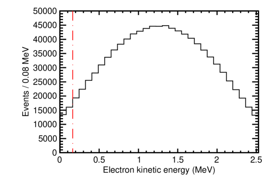
Figure 1: The spectrum in kinetic energy of one of the electrons in 0$\nu\beta\beta$- decays of ¹³⁰Te  (endpoint 2.53 MeV). The vertical dashed line indicates the Cherenkov threshold in the liquid scintillator of the detector model. Single electrons from ⁸B  solar neutrinos that are potential background to the 0$\nu\beta\beta$-decay search are close in energy to the endpoint and will be above the Cherenkov threshold.

The distribution in $\cos{(\theta)}$ between the two electrons is presented in the left-hand panel of Fig. 2 (solid line), showing the preference towards a back-to-back topology. The energy sharing between the electrons peaks at an equal split, as shown in the right-hand panel of Fig. 2 (solid line).

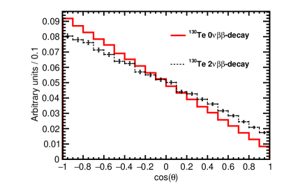
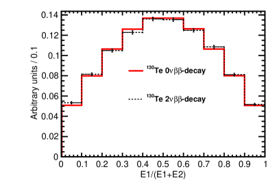
Figure 2: Left: The distribution in the cosine of the angle between the two electrons for 0$\nu\beta\beta$-decays (solid red line). Right: The fraction of the total energy carried by one of the two electrons in 0$\nu\beta\beta$-decays (solid red line). In both panels the dashed black line is the corresponding distribution for SM 2$\nu\beta\beta$-decay events with the total kinetic energy of the electrons above 95% of the Q-value.

3.2 Comparison to SM 2$\nu\beta\beta$-decay

Figure 2 also shows the angular separation and energy sharing of the two electrons in SM 2$\nu\beta\beta$-decay events with the total kinetic energy of the electrons above 95% of the Q-value, found using the same Monte Carlo generator but with SM phase space factors [22]. As seen from the plot, the electron angular correlations for 0$\nu\beta\beta$-decay are slightly more back-to-back than those from 2$\nu\beta\beta$-decay due to a contribution from the neutrino wave-functions even at vanishingly small energies of the neutrinos [22]. The energy sharing is essentially identical.

3.3 Production and Selection of Cherenkov light by electrons from ¹³⁰Te  0$\nu\beta\beta$-decays

Figure 1 also shows the threshold for the production of Cherenkov light. Examining the kinematics for one of the electrons from ¹³⁰Te  0$\nu\beta\beta$-decay with an equal energy split, the 1.26 MeV electron travels on average a total path length of 7.1$\pm$0.9 mm, has a distance from the origin of 5.6$\pm$1.0 mm in 26 $\pm$4 ps, and takes 24$\pm$3 ps to drop below Cherenkov threshold. We note that due to scattering of the electron, the final direction of the electron before it stops does not match the initial direction; however, the scattering angle is small at the time that the majority of Cherenkov light is produced.

Figure 3 shows distributions from the detector simulation for 1000 ¹³⁰Te  0$\nu\beta\beta$-decay events at the center of the detector. The left-hand panel compares the time of PE arrival at a photodetector anode for Cherenkov and scintillation light, assuming a TTS in the photodetector of 100 ps. A selection of the PEs with relatively early arrival time creates a sample with a high fraction of directional Cherenkov light, designated as the ‘early PE’ sample.

The right-hand panel shows the composition of the early PE sample, selected with a time cut of 33.5 ns (vertical line on plot). On average each ¹³⁰Te  0$\nu\beta\beta$-decay produces 62.8$\pm$0.3 PEs in the early PE sample, with an RMS width of 8.9 PEs from event-by-event fluctuations. On average the early PE sample consists of 28.6$\pm$0.2 scintillation PEs and 34.2$\pm$0.2 Cherenkov PEs, with RMS distribution widths of 5.2 and 7.3 PEs respectively.

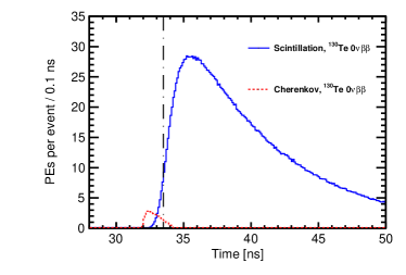
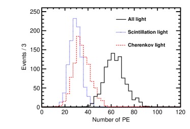
Figure 3: Left: PE arrival times after application of the photo-detector TTS of 100 ps for the default simulation of ¹³⁰Te 0$\nu\beta\beta$-decay produced at the center of the detector. Scintillation PEs (blue solid line) are compared to Cherenkov PEs (red dotted line). The vertical line at 33.5 ns indicates the time cut for the selection of the early PE sample. Right: Composition of the early PE sample (to the left of the vertical line in the left-hand panel): the number of Cherenkov (dashed red line), scintillation (dotted blue line), and total (solid black line) PEs per event.

3.4 ⁸B  solar neutrino background

For a detector similar to our model, the ⁸B solar neutrino background is significant due to the large total mass of the liquid scintillator in the active region. Electrons from elastic scattering of ⁸B solar neutrinos have nearly a flat energy spectrum around the Q-value [23]. We simulate ⁸B background as a single monochromatic electron with energy of 2.53 MeV (Q-value of ¹³⁰Te). A 2.53 MeV electron travels a total path length of 15.5$\pm$2.0 mm, has a distance from the origin of 12.6$\pm$2.2 mm in 55$\pm$7 ps, and takes 49$\pm$2 ps to drop below Cherenkov threshold.

The shape of scintillation and Cherenkov PE timing distributions in ⁸B events match very closely the shape of corresponding distributions for 0$\nu\beta\beta$-decay events shown in Fig. 3. The electron path length is too short compared to the detector size to introduce any noticeable difference in the shape of PE timing distributions between a single electron from ⁸B events and two electrons from 0$\nu\beta\beta$-events.

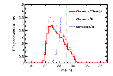
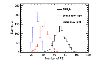
Figure 4: Left: A ‘zoomed-in’ view of the PEs arrival times of signal and background events produced at the center of the detector. The distribution in time for Cherenkov PEs from ¹³⁰Te 0$\nu\beta\beta$-decay is shown in solid black; Cherenkov PEs from ⁸B  solar neutrino background are shown in dashed red. PEs from scintillation are shown as the blue solid line. The line at 33.5 ns indicates the cut for the early PE sample selection. Right: Composition of the early PE sample: the number of Cherenkov PEs (dashed red line), scintillation PEs (dotted blue line), and total (solid black line) PEs per event.

On average each ⁸B  neutrino event produces 69.9$\pm$0.3 PEs in the early PE sample, with an RMS distribution width of 9.7 PEs due to event-by-event fluctuations. On average the early PE sample consist of 27.6$\pm$0.2 scintillation and 42.3$\pm$0.3 Cherenkov PEs, with event-by-event fluctuations contributing an RMS width of 5.2 and 8.2 PEs, respectively. The total energy deposited in the detector in ⁸B  solar neutrino and 0$\nu\beta\beta$-decay events is the same. This leads to nearly the same amount of scintillation light produced in the detector.

The number of Cherenkov photons is $\sim$10% higher for ⁸B neutrino events compared to 0$\nu\beta\beta$-decay events. This is because Cherenkov light in ⁸B  neutrino interactions is being produced by a single electron, while the same kinetic energy is split between two electrons in 0$\nu\beta\beta$-decay events .

4 Event Topology and the Spherical Harmonics Analysis

We have developed a method based on a spherical harmonics decomposition to discriminate the topologies of 0$\nu\beta\beta$-decay two-electron events and ⁸B-neutrino single-electron events. The identification of the Cherenkov photon clusters is challenging due to the smearing of the characteristic ring pattern by multiple scattering of the electrons and by the smallness of the Cherenkov signal relative to the large amount of uniformly-distributed scintillation light. We find that performing the spherical harmonics analysis on the smaller early PE sample, which has a relatively high fraction of Cherenkov PEs, can discriminate 0$\nu\beta\beta$-decay signal events from backgrounds, although a high rejection factor will require a slower scintillator than in the model.

4.1 Topology of 0$\nu\beta\beta$-decay and ⁸B Events

With ¹³⁰Te as the active isotope, all background from ⁸B solar neutrinos will have the single electron above Cherenkov threshold in the liquid scintillator. Also, a large fraction of 0$\nu\beta\beta$-decay signal events will have both electrons above Cherenkov threshold.

In some cases only one Cherenkov cluster is produced in 0$\nu\beta\beta$-decay signal events. This happens either when the angle between the two 0$\nu\beta\beta$-decay electrons is small and Cherenkov clusters overlap or when the energy split between electrons is not balanced, causing one electron to be below Cherenkov threshold. Such signal events cannot be separated from background based on the topology of the distribution of Cherenkov photons on the detector surface. However, the directionality of the electron that is above Cherenkov threshold can still be reconstructed. This directionality information may allow for suppression of ⁸B events based on the position of the sun [24].

For the purpose of illustrating the spherical harmonics analysis concept, we first consider two distinct topologies: a) two electrons produced back-to-back at an 180^∘ angle; and b) a single electron. Figure 5 shows an idealized simulation of these two topologies for a total electron energy of 2.53 MeV. In order to emphasize ring patterns formed by Cherenkov photons, the electron multiple scattering process is turned off in this idealized simulation and a photocathode QE of 30% is used for both Cherenkov and scintillation photons. Here the single-electron event represents an idealized ⁸B event topology and the two-electron events represent two special cases of an idealized 0$\nu\beta\beta$-decay topology.

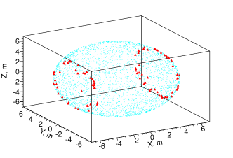
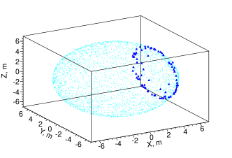
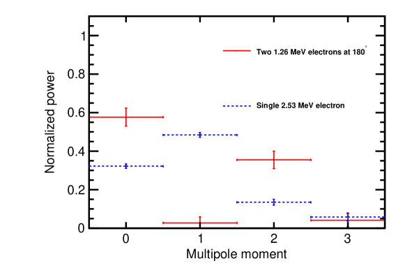
Figure 5: Top panels: Idealized event displays, with multiple scattering turned off and at the center of the detector, of: (top left) a signal event with two 1.26 MeV back-to-back electrons; and (top right) a ⁸B neutrino background event with single 2.53 MeV electron. A 30% QE is assumed for both Cherenkov PEs (triangles) and scintillation PEs (dots). Bottom panel: The normalized power spectrum $S_{\ell}$ for the Cherenkov PEs only, calculated event-by-event for 100 events for the two above topologies. The heights of the vertical bars correspond to event by event variation $(\pm 1~{}\sigma)$.

4.2 Description of the Spherical Harmonics Analysis

The central strategy of the spherical harmonics analysis is to construct rotationally invariant variables that can be used to separate different event topologies. To account for the fluctuation of the number of PEs from event to event, we use a normalized power, $S_{\ell}$, defined in Appendix A.

The bottom panel in Fig. 5 compares the normalized power spectra for the two representative event topologies in the idealized case of no multiple scattering and with a 30% quantum efficiency for both Cherenkov and scintillation photons. In this case, the method gives a good separation between the two event topologies.

At energies relevant to 0$\nu\beta\beta$-decay, multiple scattering makes the Cherenkov rings fuzzy. In most cases, $\sim$1 MeV electrons produce randomly shaped clusters of Cherenkov photons around the direction of the electron track. Examples of ¹³⁰Te  0$\nu\beta\beta$-decay and ⁸B events simulated with multiple scattering, but still at the center of the detector, are shown in Fig. 6. ¹³⁰Te  events are generated based on the phase factors described in [22]. ⁸B events are implemented as monochromatic electrons with the initial direction along the $x$-axis. The default QEs of 12% for Cherenkov light and 23% for scintillation light have been applied. Figure 6 shows early PEs that pass the 33.5 ns time cut.

In this more realistic example, the uniformly distributed scintillation light makes it difficult to visually distinguish the event topology. The power spectra shown in the bottom panel of Fig. 6  are different only at $\ell$=0 and $\ell$=1. We use this difference to separate 0$\nu\beta\beta$-decay signal from ⁸B background events.

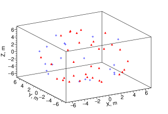
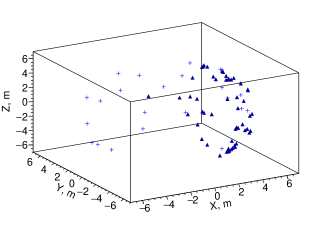
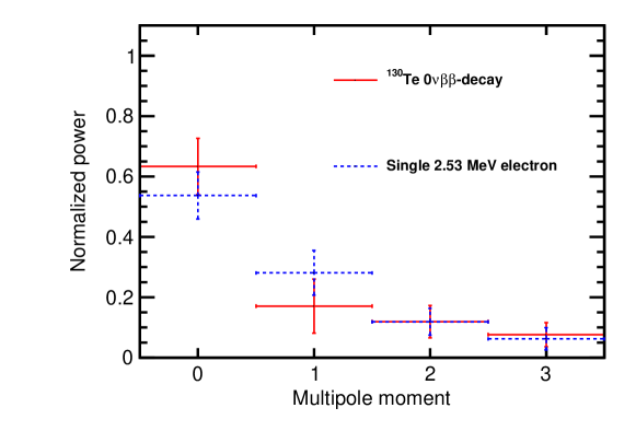
Figure 6: Top panels: Event displays with multiple scattering and at the center of the detector for: (top left) a signal event with two 1.26 MeV back-to-back electrons; and (top right) a ⁸B neutrino background event with a single 2.53 MeV electron. Only early PEs are shown. The model QEs are assumed for both Cherenkov PEs (triangles) and scintillation PEs (crosses). Bottom panel: The normalized power spectrum $S_{\ell}$ for all early PEs, calculated event-by-event for 1000 events of 0$\nu\beta\beta$-decay signal and ⁸B neutrino events. The heights of the vertical bars corespond to event by event variation $(\pm 1~{}\sigma)$.

As expected, we find that 0$\nu\beta\beta$-decay events become indistinguishable from single-track events when the angle between the two electrons is small and two Cherenkov clusters overlap. Event topologies of 0$\nu\beta\beta$-decay and ⁸B events are also very similar when only one electron from 0$\nu\beta\beta$-decay is above the Cherenkov threshold. The spherical harmonics analysis is most efficient for events with large angular separation between the two electrons and when both electrons are above Cherenkov threshold [25].

5 Performance of the Spherical Harmonics Analysis in Separating 0$\nu\beta\beta$-decay from ⁸B Background.

The separation of signal and background comes almost entirely from the first two multipole moments, $\ell$=0 and $\ell$=0. However, higher multipole moments are needed for the event-by-event normalization of the power spectrum $S_{\ell}$ (Eq. 10). In the following, we choose to calculate the power spectrum $s_{\ell}$ up to $\ell$=3 and use only the normalized variables $S_{0}$ and $S_{1}$, where the normalization is given by

$$S_{0,1}=\frac{s_{0,1}}{\sum_{l=0}^{3}s_{\ell}}.$$ (1)

As discussed below, a linear combination of $S_{0}$ and $S_{1}$ can be used to separate 0$\nu\beta\beta$-decay and ⁸B events.

5.1 Central events with no uncertainty on the vertex position

To illustrate the technique, we initially evaluate the performance of the spherical harmonics analysis in the idealized case of events at the center of the detector with perfect reconstruction of the event vertex position.

Comparisons of $S_{0}$ and $S_{1}$ distributions for ⁸²Se and ¹³⁰Te 0$\nu\beta\beta$-decay signal and corresponding ⁸B background events are shown in Fig. 7. Both variables, $S_{0}$ and $S_{1}$, provide a noticeable separation between signal and background. ⁸²Se 0$\nu\beta\beta$-decay events are shown to demonstrate that in the energy range of interest, the $S_{\ell}$ do not strongly depend on the energy deposited in the detector, i.e. information contained in the normalized power spectrum is complimentary to the energy measurements.

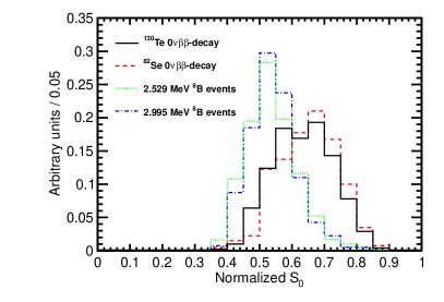
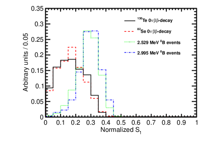
Figure 7: Results from the idealized case of central events at the detector origin( i.e. perfect vertex reconstruction); a time cut of 33.5 ns on the PE arrival time is applied. The default QE and 100% photo-coverage are used in the simulation. (Left) $S_{0}$ and $S_{1}$ (right) distributions for 1000 simulated 0$\nu\beta\beta$-decay signal and ⁸B background events. Two different isotopes are compared, ¹³⁰Te and ⁸²Se. The corresponding kinetic energies of background ⁸B neutrino single electrons are 2.53 MeV and 3.00 MeV.

The left-hand panel in Fig. 8 compares scatter plots of the first two components of the power spectrum, $S_{0}$ and $S_{1}$, for signal and background. In order to illustrate the separation between ¹³⁰Te and ⁸B events, a linear combination of variables $S_{0}$ and $S_{1}$ is constructed as follows .

First, we perform a linear fit to $S_{0}$ = $A\cdot S_{1}+B$, of all points on the scatter plot, as shown by the dashed line in the left-hand panel in Fig. 8. A 1-dimensional (1-D) variable $S_{01}$ is defined as $S_{01}=S_{1}\cdot\cos(\theta)+S_{0}\cdot\sin(\theta)$, where $\tan(\theta)$=$A$. The right-hand panel in Fig. 8 compares distributions of $S_{01}$ for 0$\nu\beta\beta$-decay signal and ⁸B background. These 1-D histograms for $S_{01}$ represent the projection of the points on the scatter plot onto the fitted line.

To quantify the separation between the signal and background we calculate the area of the overlap in the $S_{01}$ distributions, $I_{overlap}$. There is no separation if $I_{overlap}$=1, and there is a 100% separation if $I_{overlap}$=0. Figure 8 shows the separation of this simple algorithm based on the shape of the early PE sample; the overlap between signal and background is $I_{overlap}$=0.52. At an efficiency for the signal of 70% we find a rejection factor of 4.6.

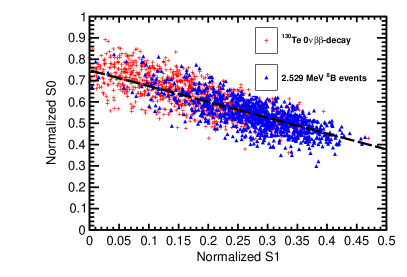
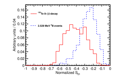
Figure 8: Left: Scatter plot of the moments $S_{0}$ versus $S_{1}$ for a simulation of 1000 signal (red crosses) and background (blue triangles), for the idealized case of central events assuming perfect reconstruction of the vertex position. A time cut of 33.5 ns on the PE arrival time is applied. The default QE and 100% photo-coverage is used in the simulation. The black dashed line corresponds to a linear fit for $S_{01}$. Right: Comparison of the $S_{01}$ distribution between signal (red solid line) and background (blue dashed line). $I_{overlap}$=0.52.

5.2 Events in a fiducial volume with an uncertainty on the vertex position

We find that in the default detector model the separation power of the spherical harmonics analysis is significantly reduced when event vertex is not at the center of the detector and vertex resolution is taken into account.

For the general case, even significantly delayed scintillation photons can reach the side of the detector that is closer to the vertex much earlier than Cherenkov photons traveling to the opposite side of the detector. The time cut thus has to take into account the total distance traveled by each individual photon. In order to select early PE sample we use a differential cut of $\Delta t=t^{phot}_{measured}-t^{phot}_{predicted}<$1 ns, where $t^{phot}_{measured}$ is the measured time of the photon hit and $t^{phot}_{predicted}$ is the predicted time based on the reconstructed vertex position.

In general, the $S_{1}$ component of the spherical harmonics power spectrum is higher for asymmetric distributions and lower for symmetric distributions (e.g., compare the back-to-back and single electron topologies in Fig. 5). If a vertex is shifted in the direction opposite to the track of the electron, the differential time cut selects more scintillation photons that are emitted in the direction of the electron track. Scintillation photons would enhance the forward asymmetry of the early PE sample, which in turn would move $S_{1}$ to higher values. Moreover, $S_{1}=$ 0 for a distribution with perfect symmetry with respect to the center of the sphere. If a vertex is shifted in the same direction as the direction of the electron, the differential time cut selects more scintillation photons that are emitted in the direction opposite to the electron track. The asymmetry of Cherenkov PEs would then be counter-balanced by scintillation PEs, which in turn, would move $S_{1}$ to lower values.

We simulated 1000 signal and background events that have their vertices uniformly distributed within a fiducial volume of $R<3$ m, where $R$ is the distance between the event vertex and the center of the detector, with a vertex resolution of 5.2 cm based on our earlier study of reconstruction[9]. The uncertainty on the vertex reconstruction is implemented as smearing along $x$, $y$, and $z$ directions with three independent Gaussian distributions of the same width, $\sigma_{x}=\sigma_{y}=\sigma_{z}=$3 cm.

Figure 9 shows the performance of the spherical harmonics analysis under these more realistic assumptions. The overlap between signal and background is $I_{overlap}$=0.79, which means that the separation is 52% worse than in an idealized scenario shown in Fig. 8. The spherical harmonics analysis brings little separation between signal and background in our default detector model after the chromatic dispersion and vertex resolution are taken into account. However, properties of the liquid scintillator can be adjusted to improve the performance of the spherical harmonics analysis. In the following we show that a single change in the scintillation rise time improves the separation.

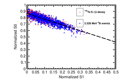
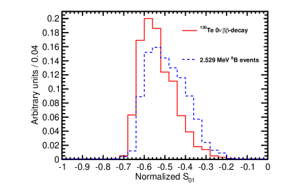
Figure 9: Left: Scatter plot of $S_{0}$ versus $S_{1}$ for a simulation of 1000 signal (red crosses) and background (blue triangles) events. Event vertices are uniformly distributed within the fiducial volume, $R<3$ m. The vertex is smeared with 5.2 cm resolution. A differential cut of $\Delta t=t^{phot}_{measured}-t^{phot}_{predicted}<$1 ns is applied to select the early PE sample. The default QE and 100% photo-coverage are used in the simulation. The black dashed line corresponds to a linear fit to define the 1-D variable $S_{01}$. Right: A comparison of the $S_{01}$ distribution between signal (red solid line) and background (blue dashed line). $I_{overlap}$=0.79.

5.3 Importance of the liquid scintillator properties

The strong dependence on the vertex resolution can be addressed by choosing a liquid scintillator mixture with a more delayed emission of scintillation light with respect to Cherenkov light. With a larger delay in scintillation light, a higher fraction of Cherenkov light can be maintained in the early PE sample even if the vertex position is mis-reconstructed. In addition, if the fraction of scintillation light is small compared to Cherenkov light, the distortions in the uniformity of the scintillation PE due to a shifted reconstructed vertex position does not significantly affect the spherical harmonics power spectrum. Furthermore, the effects due to chromatic dispersion can be addressed by using liquid scintillators with a narrower emission spectrum [9], or red-enhanced photocathodes [9].

While the default detector model assumes a scintillation rise time of $\tau_{r}=$1 ns, rise times up to $\tau_{r}=$7 ns can be achieved (see Ref. [27]). As a test we increased the scintillation rise time parameter to $\tau_{r}=$5 ns in the detector model, with all other parameters kept the same. Figure  10 shows the overlap between signal and background is significantly decreased to $I_{overlap}$=0.64, i.e. the separation is 23% worse than in the idealized scenario shown in Fig. 8 and 23% better than in the default detector model shown in Fig. 9.

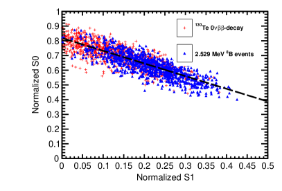
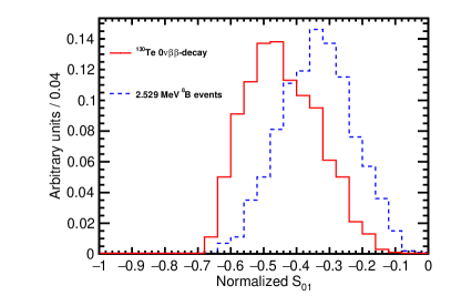
Figure 10: The scintillation rise time constant is increased to $\tau_{r}=$5 ns compared to $\tau_{r}=$1 ns in the default detector model. Left: Scatter plot of $S_{0}$ versus $S_{1}$ for a simulation of 1000 signal (red crosses) and background (blue triangles) events. Event vertices are uniformly distributed within the fiducial volume, $R<3$ m. Vertex is smeared with 5.2 cm resolution. Differential cut of $\Delta t=t^{phot}_{measured}-t^{phot}_{predicted}<$1 ns is applied to select early PE sample. The default QE and 100% photo-coverage is used in the simulation. Black dashed line corresponds to a linear fit to define 1-D variable $S_{01}$ (see text for details). Right: Comparison of the $S_{01}$ distribution between signal (red solid line) and background (blue dashed line). $I_{overlap}$=0.64.

Figure 11 shows the efficiency for 0$\nu\beta\beta$-decay signal and the rejection factor for ⁸B  neutrino background for the default model (left-hand panel) and for the slower scintillator with a 5-ns risetime (right-hand panel) as a function of the $S_{01}$ discriminant. We find a rejection factor of 2 for the default case at 70% efficiency for signal. The rejection is increased to a factor of 3 for the 5-nsec risetime scintillator.

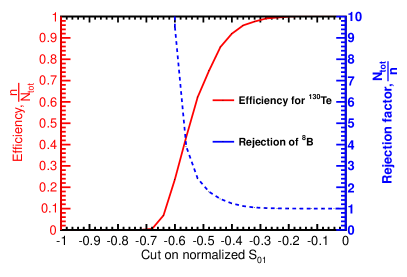
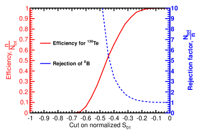
Figure 11: The efficiency for 0$\nu\beta\beta$-decay signal (red left-hand-scale) and the rejection factor for ⁸B neutrino background (blue right-hand-scale) versus $S_{01}$ for the default model (left panel) and a liquid scintillator with a 5-nsec risetime (right panel).

6 Conclusions

We consider the use of large-area photodetectors with good time and space resolution in kiloton scale liquid scintillator detectors to suppress background coming from ⁸B solar neutrino interactions. Using a default model detector with parameters derived from present practice, we show that a sample of detected photons enriched in Cherenkov light by a cut on time-of-arrival contains directional information that can be used to separate 0$\nu\beta\beta$-decay from ⁸B solar neutrino interactions. The separation is based on a spherical harmonics analysis of the event topologies of the two electrons in signal events and the single electron in the background. The performance of the technique is constrained by chromatic dispersion, vertex reconstruction, and the time profile of the emission of scintillation light. The development of a scintillator with a rise time constant of at least 5 ns would allow a Cherenkov-scintillation light separation with a background rejection factor for ⁸B  solar neutrinos of 3 and an efficiency for 0$\nu\beta\beta$-decay signal of 70%.

Appendix A Appendix A

A.1 Defining the Power Spectrum

Let the function $f(\theta,\phi)$ represent the distribution of the photo-electrons (PE) on the detector surface. The function $f(\theta,\phi)$ can be decomposed into a sum of spherical harmonics:

$$f(\theta,\phi)=\sum_{\ell=0}^{\infty}\sum_{m=-\ell}^{\ell}f_{\ell m}Y_{\ell m}(\theta,\phi),$$ (2)

where $Y_{\ell m}$ are Laplace’s spherical harmonics defined in a real-value basis using Legendre polynomials $P_{\ell}$ [29]:

$$Y_{\ell m}=\left\{\begin{array}[]{@{}ll@{}}\sqrt{2}N_{\ell m}P_{\ell}^{m}(\cos\theta)\cos~{}m\phi,&\text{if}\ m>0\\ N_{\ell m}=\sqrt{\frac{(2\ell+1)}{4\pi}\frac{(\ell-m)!}{(\ell+m)!}},&\text{if}\ m=0\\ \sqrt{2}N_{\ell|m|}P_{\ell}^{|m|}(\cos\theta)\sin~{}|m|\phi,&\text{if}\ m<0\end{array}\right.$$ (6)

where the coefficients $f_{\ell m}$ are defined as

$$f_{\ell m}=\int_{0}^{2\pi}d\phi\int_{0}^{\pi}d\theta\sin\theta f(\theta,\phi)Y_{\ell m}(\theta,\phi).$$ (7)

Equation 8 defines the power spectrum of $f(\theta,\phi)$ in the spherical harmonics representation, $s_{\ell}$, where $l$ is a multipole moment. The power spectrum, $s_{\ell}$, is invariant under rotation.

$$s_{\ell}=\sum_{m=-\ell}^{m=\ell}|f_{\ell m}|^{2}$$ (8)

The event topology in a spherical detector determines the distribution of the PE’s on the detector sphere, and, therefore, a set of $s_{\ell}$’s. These values can serve as a quantitative figure of merit for different event topologies. The rotation invariance of the $s_{\ell}$’s ensures that this figure of merit does not depend on the orientation of the event with respect to the chosen coordinate frame.

The sum of $s_{\ell}$’s over all multipole moments equals to the $L^{2}$ norm of the function $f(\theta,\phi)$:

$$\sum_{\ell=0}^{\infty}s_{\ell}=\int_{\Omega}|f(\theta,\phi)|^{2}d\Omega.$$ (9)

The normalized power spectrum is thus:

$$\mathcal{S}_{\ell}=\frac{s_{\ell}}{\sum_{\ell=0}^{\infty}s_{\ell}}=\frac{s_{\ell}}{\int_{\Omega}|f(\theta,\phi)|^{2}d\Omega},$$ (10)

and can be used to compare the shapes of various functions $f(\theta,\phi)$ with different normalizations. As the total number of PEs detected on the detector sphere fluctuates from event to event we use the normalized power $\mathcal{S}_{\ell}$.

A.2 Spherical Harmonics Analysis and Off-center Events

In general, events with the same event topology result in the same the power spectrum $S_{\ell}$ only if events originate in the center of the detector. In order to compare the spherical harmonics for events with verticies away from the center, a coordinate transformation for each photon hit is needed. The necessary transformation applied for each PE within an event is illustrated in Fig. 12. The solid circle in Fig. 12 has a radius R and shows the actual detector boundaries. The dotted circle shows a new sphere with the same radius R, which now has the event vertex in its center. The radius vector of each PE is stretched or shortened to its intersection with this new sphere using the transformation, $\vec{r}^{,}_{PE}=\frac{\vec{a}}{|\vec{a}|}\cdot R$, where $\vec{r}^{,}_{PE}$ is a new radius vector of a PE and $\vec{a}=\vec{r}_{PE}-\vec{r}_{vtx}$ with $\vec{r}_{PE}$ and $\vec{r}_{vtx}$ being radius vectors of the PE and the vertex in the original coordinates, respectively.

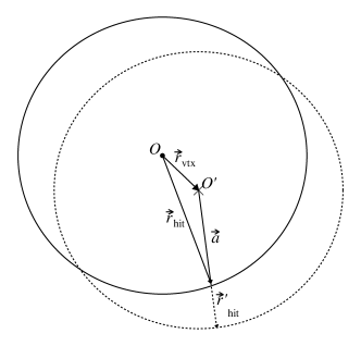
Figure 12: The coordinate transformation which is applied to events that are off-center. The solid circle schematically shows the actual detector boundaries. The dotted circle shows a new sphere of radius R$=$6.5 m with the event vertex position in the center. The radius vector of each photon hit is stretched or shortened until the intersection with this new sphere using the transformation $\vec{r}^{,}_{hit}=\frac{\vec{a}}{|\vec{a}|}\cdot R$, where $\vec{r}^{,}_{hit}$ is a new radius vector of the photon hit, $R$ is detector sphere radius, and $\vec{a}=\vec{r}_{hit}-\vec{r}_{vtx}$ with $\vec{r}_{hit}$ and $\vec{r}_{vtx}$ being the radius vectors of the photon hit and vertex position in original coordinates, respectively.

References

- Olive et al. [2014] K. A. Olive, et al. (Particle Data Group), Review of Particle Physics, Chin. Phys. C38 (2014) 090001.
- Majorana [1937] E. Majorana, Nuovo Cim. 14 (1937) 171–184.
- Furry [1939] W. H. Furry, Phys. Rev. 56 (1939) 1184–1193.
- Goeppert-Mayer [1935] M. Goeppert-Mayer, Phys. Rev. 48 (1935) 512–516.
- Gando et al. [2016] A. Gando, et al. (KamLAND-Zen), Phys. Rev. Lett. 117 (2016) 082503.
- NSA [2015] 2015 NSAC Long Range Plan, 2015. URL: http://science.energy.gov/~/media/np/nsac/pdf/2015LRP/2015_LRPNS_091815%.pdf.
- Gando et al. [2013] A. Gando, et al. (KamLAND-Zen), Phys. Rev. Lett. 110 (2013) 062502.
- Biller [2013] S. D. Biller, Phys. Rev. D 87 (2013) 071301.
- Aberle et al. [2014] C. Aberle, A. Elagin, H. J. Frisch, M. Wetstein, L. Winslow, J. Instrum. 9 (2014) P06012.
- Eguchi et al. [2003] K. Eguchi, et al., Phys. Rev. Lett. 90 (2003) 021802.
- Tajima [2000] O. Tajima, Master’s thesis, Tohoku University, 2000.
- Perevozchikov [2009] O. Perevozchikov, Ph.D. thesis, University of Tennessee, 2009.
- Grant [2012] C. Grant, Ph.D. thesis, University of Alabama, 2012.
- Aberle [2011] C. Aberle, Ph.D. thesis, University of Heidelberg, 2011.
- Tajima [2003] O. Tajima, Ph.D. thesis, Tohoku University, 2003.
- Ham [2013] Hamamatsu Photonics K.K., Large Photocathode Area Photomultiplier Tubes (data sheet, including R7081), 2013. http://www.hamamatsu.com/resources/pdf/etd/LARGE_ AREA_PMT_TPMH1286E05.pdf.
- Abe et al. [2012] Y. Abe, et al. (Double Chooz), Phys. Rev. D86 (2012) 052008.
- Orlov et al. [2016] D. A. Orlov, J. DeFazio, S. Duarte Pinto, R. Glazenborg, E. Kernen, JINST 11 (2016) C04015.
- Smedley [2016] J. Smedley, private communication, 2016.
- Cultrera [2016] L. Cultrera, private communication, 2016.
- Adams et al. [2015] B. Adams, et al., Nucl.Instrum.Meth. A795 (2015) 1–11.
- Kotila and Iachello [2012] J. Kotila, F. Iachello, Phys. Rev. C 85 (2012) 034316.
- Maio [2015] A. Maio (SNO), J. Phys. Conf. Ser. 587 (2015) 012030.
- Alonso et al. [2014] J. R. Alonso, et al., arXiv 1409.5864 (2014).
- fur [2014] 2014. Being able to distinguish between two-tracks and single-track events using the spherical analysis can allow further cuts to be made. For example, one might use absolute directional information to suppress single track events where the direction of the track is consistent with the location of a known background such as the sun [24]. Once a single track topology is established, one can use a centroid method (see Ref. [9]) to reconstruct directionality of the track (or two degenerate tracks) in order to suppress events that are aligned with the direction of 8B solar neutrinos.
- M.L. Goldberger and K. M. Watson [1964] M.L. Goldberger and K. M. Watson, Collision Theory, Wiley, New York, 1964. See proofs of dispersion relations.
- Li et al. [2016] M. Li, Z. Guo, M. Yeh, Z. Wang, S. Chen, Nucl. Instrum. Meth. A830 (2016) 303–308.
- Yeh [2016] M. Yeh, private communication, 2016.
- leg [2014] Legendre polynomials are calculated using the gnu scientific library, 2014. URL: http://www.gnu.org/software/gsl/, version 1.9.