A Legendre-Fourier spectral method with exact conservation laws for the Vlasov-Poisson system

Abstract

We present the design and implementation of an $L^{2}$-stable spectral method for the discretization of the Vlasov-Poisson model of a collisionless plasma in one space and velocity dimension. The velocity and space dependence of the Vlasov equation are resolved through a truncated spectral expansion based on Legendre and Fourier basis functions, respectively. The Poisson equation, which is coupled to the Vlasov equation, is also resolved through a Fourier expansion. The resulting system of ordinary differential equation is discretized by the implicit second-order accurate Crank-Nicolson time discretization. The non-linear dependence between the Vlasov and Poisson equations is iteratively solved at any time cycle by a Jacobian-Free Newton-Krylov method. In this work we analyze the structure of the main conservation laws of the resulting Legendre-Fourier model, e.g., mass, momentum, and energy, and prove that they are exactly satisfied in the semi-discrete and discrete setting. The $L^{2}$-stability of the method is ensured by discretizing the boundary conditions of the distribution function at the boundaries of the velocity domain by a suitable penalty term. The impact of the penalty term on the conservation properties is investigated theoretically and numerically. An implementation of the penalty term that does not affect the conservation of mass, momentum and energy, is also proposed and studied. A collisional term is introduced in the discrete model to control the filamentation effect, but does not affect the conservation properties of the system. Numerical results on a set of standard test problems illustrate the performance of the method.

1 Introduction

Collisionless magnetized plasmas are described by the kinetic (Vlasov-Maxwell) equations and are characterized by high dimensionality, anisotropy and a wide variety of spatial and temporal scales [15], thus requiring the use of sophisticated numerical techniques to capture accurately their rich non-linear behavior.

In general terms, there are three broad classes of methods devoted to the numerical solution of the kinetic equations. dimensional phase space via macro-particles that evolve according to Newton’s equations in the self-consistent electromagnetic field [3, 16]. PIC is the most widely used method in the plasma physics community because of its robustness and relative simplicity. The well known statistical noise associated with the macro-particles implies that PIC is really effective for problems where a low signal-to-noise ratio is acceptable. The Eulerian-Vlasov methods discretize the phase space with a six dimensional computational mesh [8, 30, 13]. As such they are immune to statistical noise but they require significant computational resources and this is perhaps why their application has been mostly limited to problems with reduced dimensionality. For reference, storing a field in double precision on a mesh with $10^{12}$ cells requires about $8$ terabytes of memory. A third class of methods, called transform methods, is spectral and is based on an expansion of the velocity part of the distribution function in basis functions (typically Fourier or Hermite), leading to a truncated set of moment equations for the expansion coefficients [2, 12, 18, 17, 29]. Similarly to Eulerian-Vlasov methods, transform methods might be resource-intensive if the convergence of the expansion series is slow.

In recent years there seems to be a renewed interest in Hermite-based spectral methods. Some reasons for this can be attributed to the advances in high performance computing and to the importance of simpler, reduced kinetic models in elucidating aspects of the complex dynamics of magnetized plasmas [27, 22]. Another reason is that (some form of) the Hermite basis can unify fluid (macroscopic) and kinetic (microscopic) behavior into one framework [5, 34, 11, 35]. Thus, it naturally enables the ’fluid/kinetic coupling’ that might be the (inevitable) solution to the multiscale problem of computational plasma physics and is a very active area of research [24, 10].

The Hermite basis is defined by the Hermite polynomials with a Maxwellian weight and is therefore closely linked to Maxwellian distribution functions. Two kinds of basis have been proposed in the literature (differing in regard to the details of the Maxwellian weight): symmetrically- and asymmetrically-weighted [17, 29]. The former features $L^{2}$-stability but conservation laws for total mass, momentum and energy are achieved only in limited cases (i.e., they depend on the parity of the total number of Hermite modes, on the presence of a velocity shift in the Hermite basis, …). The latter features exact conservation laws in the discrete and the connection between the low-order moments and typical fluid moments, but $L^{2}$-stability is not guaranteed [4, 29]. Earlier works pointed out that a proper choice of the velocity shift and the scaling of the Maxwellian weight (free parameters of the method) is important to improve the convergence properties of the series [17, 5]. Indeed, the optimization of the Hermite basis is a crucial aspect of the method, which however at this point does not yet have a definitive solution.

One could of course envision a different spectral approach which considers a full polynomial expansion without any weight or free parameter. While any connection with Maxwellians is lost, such expansion could be of interest in presence of strong non-Maxwellian behavior and eliminates the optimization problem. The Legendre polynomials are a natural candidate in this case, because of their orthogonality properties. They are normally applied in some preferred coordinate system (for instance spherical geometry) to expose quantities like angles that are defined on a bounded domain. Indeed, Legendre expansions are very popular in neutron transport [28] and some application in kinetic plasma physics can be found for electron transport described by the Boltzmann equation [31]. Surprisingly, however, we have not found any example in the context of collisionless kinetic theory and in particular for the Vlasov-Poisson system.

The main contribution of the present paper is the formulation, development and successful testing of a spectral method for the one dimensional Vlasov-Poisson model of a plasma based on a Legendre polynomial expansion of the velocity part of the plasma distribution function. The expansion is applied directly in the velocity domain, which is assumed to be finite. It is shown that the Legendre expansion features many of the properties of the asymmetrically-weighted Hermite expansion: the structure of the equations is similar, the low-order moments correspond to the typical moments of a fluid, and conservation laws for the total mass, momentum and energy (in weak form, as defined in Sec. 4) can be proven. It also features properties of the symmetrically-weighted Hermite expansion: $L^{2}$-stability is also achieved by introducing a penalty on the boundary conditions in weak form. This strategy is inspired by the Simultaneous Approximation Strategy (SAT) technique  [33, 20, 21, 32, 6, 26, 7, 25].

The paper is organized as follows. In Sec. 2 the Vlasov-Poisson equations for a plasma are introduced together with the spectral discretization: the velocity part of the distribution function is expanded in Legendre polynomials while the spatial part is expressed in terms of a Fourier series. The time discretization is handled via a second-order accurate Crank-Nicolson scheme. In Sec. 3 the SAT technique is used to enforce the $L^{2}$-stability of the numerical scheme. In Sec. 4 conservation laws for the total mass, momentum and energy are derived theoretically. Numerical experiments on standard benchmark tests (i.e., Landau damping, two-stream instabilities and ion acoustic wave) are performed in Sec. 5, proving numerically the stability of the method and the validity of the conservation laws. Conclusions are drawn in Sec. 6.

2 The Vlasov-Poisson system and the Legendre-Fourier approximation

We consider the Vlasov-Poisson model for a collisionless plasma of electrons (labeled “$e$”) and singly charged ions (“$i$”) evolving under the action of the self-consistent electric field $E$. The behavior of each particle species $s\in\{e,i\}$ with mass $m^{s}$ and charge $q^{s}$ is described at any time $t\geq 0$ in the phase space domain $[0,L]\times[v_{a},v_{b}]$ by the distribution function $f^{s}(x,v,t)$, which evolves according to the Vlasov equation:

$$\frac{\partial f^{s}}{\partial t}+v\frac{\partial f^{s}}{\partial x}+\frac{q^{s}}{m^{s}}E\,\frac{\partial f^{s}}{\partial v} =0.$$ (1)

We assume the physical space to be periodic in $x$, so that no boundary condition for $f^{s}$ is necessary at $x=0$ and $x=L$, and that suitable boundary conditions, e.g., $f^{s}(x,v_{a},t)=f^{s}(x,v_{b},t)=0$, are provided for $f^{s}$ at the velocity boundaries $v=v_{a}$ and $v=v_{b}$ for any time $t\geq 0$ and any spatial position $x\in[0,L]$. We also assume that an initial solution $f^{s}(x,v,0)=f^{s}_{0}(x,v)$ is given at the initial time $t=0$.

Remark 2.1

If the initial solution $f^{s}_{0}(x,v)$ has a compact support in the phase space domain $[0,L]\times[v_{a},v_{b}]$, then $f^{s}$ has also a compact support at any time $t>0$. Moreover, the size of the support may increase in time in a controlled way, cf. [36, 14]. In such a case, it holds that $f^{s}(x,v_{a},t)=f^{s}(x,v_{b},t)=0$ until the size of the support equals the size of the velocity domain. This condition can be used to determine the final time at which a plasma simulation based on this numerical model is valid.

In the Vlasov-Poisson system, the electric field $E(x,t)$ is the solution of the Poisson equation:

$$\epsilon_{0}\frac{\partial E}{\partial x}=\rho\qquad\text{for~{}}x\in(0,L),\,t\geq 0,$$ (2)

where $\epsilon_{0}$ is the dielectric constant and

$$\rho(x,t)=\sum_{s\in\{e,i\}}q_{s}\int_{-\infty}^{\infty}f^{s}(x,v,t)\,dv$$ (3)

is the total charge density of the plasma. By taking the time derivative of the Poisson equation and using the continuity equation

$$\frac{\partial\rho}{\partial t}+\frac{\partial J}{\partial x}=0,$$

where $J(x,t)$ is the total current density defined as

$$J(x,t)=\sum_{s\in\{e,i\}}q^{s}\int_{-\infty}^{\infty}vf^{s}(x,v,t)\,dv,$$ (4)

we obtain the Ampere equation

$$\epsilon_{0}\frac{\partial E}{\partial t}+J=C_{A},$$ (5)

where $C_{A}$ is a suitable constant factor.

Remark 2.2

The Ampere equation can be used with the Vlasov equation instead of the Poisson equation to obtain the Vlasov-Ampere formulation. In the continuum setting, the two formulations are equivalent in the one-dimensional electrostatic case without any external electric field as the one considered in this work.

2.1 Velocity integration using Legendre expansion

Consider the infinite set of Legendre polynomials $\{L_{n}(\eta)\}_{n=0}^{\infty}$, which are recursively defined for $\eta\in[-1,1]$ by [1, Chapters 8, 22]:

$$L_{0}(\eta)=1,\quad L_{1}(\eta)=\eta,\quad(2n+1)\eta L_{n}(\eta)=(n+1)L_{n+1}(\eta)+nL_{n-1}(\eta)\textrm{~{}~{}for~{}}n\geq 1,$$ (6)

and normalized as follows

$$\int_{-1}^{1}L_{m}(\eta)L_{n}(\eta)ds=\frac{2}{2n+1}\delta_{mn}.$$ (7)

We remap the Legendre polynomials onto the velocity range $[v_{a},v_{b}]$ through the linear transformation $v(\eta)=(v_{a}+v_{b})/{2}+\eta(v_{b}-v_{a})/{2}$. Let $\eta(v)=(2v-(v_{a}+v_{b}))/{(v_{b}-v_{a})}$ be the inverse mapping from $[v_{a},v_{b}]$ to $[-1,1]$. The $n$-th Legendre polynomial is given by $\phi_{n}(v)=\sqrt{2n+1}L_{n}(\eta(v))$, where the scaling factor in front of $L_{n}$ is chosen to satisfy the orthogonality relation:

$$\int_{v_{a}}^{v_{b}}\phi_{m}(v)\phi_{n}(v)dv=(v_{b}-v_{a})\delta_{mn}.$$ (8)

The first derivative of the Legendre polynomials is given by

$$\frac{dL_{n}(\eta)}{d\eta}=\sum_{i=0}^{n-1}\pi_{n,i}(2i+1)L_{i}(\eta)\qquad\eta\in[-1,1],$$

where $\pi_{n,i}$ is a switch that takes value $0$ if $n-i$ is even, and $1$ if $n-i$ is odd. Using the chain rule and adjusting the normalization factor, we obtain the first derivative of the translated and rescaled Legendre polynomials:

$$\frac{d\phi_{n}}{dv}=\sqrt{2n+1}\frac{d}{dv}L_{n}(\eta(v))=\sum_{i=0}^{n-1}\sigma_{n,i}\phi_{i}(v)\quad\textrm{~{}with~{}}\quad\sigma_{n,i}=\pi_{n,i}\,\frac{2\sqrt{\big{(}2n+1\big{)}\,\big{(}2i+1\big{)}}}{v_{b}-v_{a}}.$$ (9)

The recursion relations that are used to expand the Vlasov equation on the Legendre basis are reported in appendix A for completeness.

Consider the spectral decomposition of the distribution function $f^{s}$ on the basis of Legendre polynomials given by

$$f^{s}(x,v,t)=\sum_{n=0}^{\infty}C^{s}_{n}(x,t)\phi_{n}(v)\quad\textrm{~{}where~{}}\quad C^{s}_{n}(x,t)=\frac{1}{v_{b}-v_{a}}\int_{v_{a}}^{v_{b}}f^{s}(x,v,t)\phi_{n}(v)dv$$ (10)

in the Vlasov equation (1). The boundary conditions $f^{s}(x,v_{a},t)=f^{s}(x,v_{b},t)=0$ are not exactly satisfied since they are imposed in weak form and the polynomials $\phi_{n}(v)$ are not zero at the velocity boundaries.

A possible way to circumvent this issue is to consider the modified basis functions given by $\tilde{\phi}_{n}=\phi_{n+2}-\phi_{n}$ for $n\geq 0$. From the properties of the Legendre polynomials, it readily follows that $\tilde{\phi}_{n}(v_{a})=\tilde{\phi}_{n}(v_{b})=0$ for each $n$ and the expansion of $f^{s}$ on this set of functions will automatically satisfied the homogeneous conditions at the boundary of the velocity range. Nonetheless, we verified numerically in the first stages of this work that this approach may yield an unstable method and the numerical instability cannot be fixed as there is no mechanism that allows us to control the growth of the absolute value of the Legendre coefficients $C^{s}_{n}$. Another possible choice is to consider $\tilde{\phi}_{n}(v)=\phi_{n+2}(v)-1$ for even $n\geq 0$ and $\tilde{\phi}_{n}(v)=\phi_{n+2}(v)-v$ for odd $n\geq 1$. Although we have not implemented this second basis, a common characteristic of these choices is the loss of orthogonality, which we suspect may influence negatively the stability properties of the method. The alternative approach that we consider hereafter is to integrate by parts the velocity term in the Vlasov equations. This strategy allows us to set the boundary conditions in weak form, and, then, to introduce a penalty term to enforce the $L^{2}$ stability of the method through the boundary conditions (see Section 3). To this end, we substitute (10) into (1), we multiply the resulting equation by $\phi_{n}$ and integrate over $[v_{a},v_{b}]$. Then, we use the recursion formulas (81a)-(81c) and the orthogonality relation (7) and we obtain the following system of partial differential equations for the Legendre coefficients $C^{s}_{n}(x,t)$:

$$\frac{\partial C^{s}_{n}}{\partial t}+\sigma_{n+1}\frac{\partial C^{s}_{n+1}}{\partial x}+\sigma_{n}\frac{\partial C^{s}_{n-1}}{\partial x}+\overline{\sigma}\frac{\partial C^{s}_{n}}{\partial x}-\frac{q^{s}}{m^{s}}E\left(\sum_{i=0}^{n-1}\sigma_{n,i}C^{s}_{i}-\delta_{v}\big{[}f^{s}\phi_{n}\big{]}_{v_{a}}^{v_{b}}\right)=0\quad\textrm{for~{}}n\geq 0,$$ (11)

where conventionally $C^{s}_{-1}=0$,

$$\overline{\sigma}=\frac{v_{a}+v_{b}}{2},\qquad\sigma_{n}=\begin{cases}0&\textrm{for~{}}n=0,\\[5.0pt] \displaystyle\frac{v_{b}-v_{a}}{2}\,\frac{n}{\sqrt{(2n+1)(2n-1)}}&\textrm{for~{}}n\geq 1,\end{cases}$$ (12)

and

$$\delta_{v}\big{[}f^{s}\phi_{n}\big{]}_{v_{a}}^{v_{b}}=\frac{f^{s}(x,v_{b},t)\phi_{n}(v_{b})-f^{s}(x,v_{a},t)\phi_{n}(v_{a})}{v_{b}-v_{a}},$$ (13)

is the boundary term resulting from an integration by parts of the integral term that involves the velocity derivative. The derivation of the coefficients $\sigma_{n}$ and $\overline{\sigma}$ can be found in appendix A. If the distribution $f^{s}(x,v,t)$ has compact support in $v$, the homogeneous boundary conditions at $v=v_{a}$ and $v=v_{b}$ are imposed in weak form by assuming that $\delta_{v}\big{[}f^{s}\phi_{n}\big{]}_{v_{a}}^{v_{b}}$ in (13) is zero. However, since this term plays a major role in establishing the conservation laws and ensuring the $L^{2}$ stability of the discretization method, we will consider it in all the further developments and in the analysis of the next sections.

We truncate the spectral expansion of $f^{s}$ after the first $N_{L}$ Legendre modes by assuming that $C^{s}_{n}=0$ for $n\geq N_{L}$ and we approximate the distribution function by the finite summation:

$$f^{s}(x,v,t)\approx f^{s}_{L}(x,v,t)=\sum_{n=0}^{N_{L}-1}C^{s}_{n}(x,t)\phi_{n}(v).$$ (14)

The evolution of each coefficient $C^{s}_{n}$ with $n\leq N_{L}-1$ is still given by (11). To ease the notation, we will drop the subindex $L$ in $f^{s}_{L}$ by tacitly assuming that all the quantities containing $f^{s}$ are indeed numerical approximations dependent on the first $N_{L}$ modes of the truncated series.

Let $\mathbf{C}$ be the vector that contains all the coefficients $C^{s}_{n}$ for $n\in[0,N_{L}-1]$, i.e., $(\mathbf{C}^{s})_{n}=C^{s}_{n}$, and ${\bm{\phi}(v)=(\phi_{0}(v),\phi_{1}(v),\ldots,\phi_{N_{L}-1}(v))^{T}}$ the vector containing the values of the Legendre shape functions evaluated at $v$. It holds that $f^{s}(x,v,t)={\bm{\phi}(v)}^{T}\mathbf{C}^{s}(x,t)$. System (11) can be rewritten in the non-conservative vector form:

$$\frac{\partial\mathbf{C}^{s}}{\partial t}+\mathbbm{A}\frac{\partial\mathbf{C}^{s}}{\partial x}-\frac{q^{s}}{m^{s}}E\left(\mathbbm{B}\mathbf{C}^{s}-\delta_{v}\big{[}f^{s}{\bm{\phi}}\big{]}_{v_{a}}^{v_{b}}\right)=0,$$ (15)

where

$$\left(\mathbbm{A}\frac{\partial\mathbf{C}^{s}}{\partial x}\right)_{n} =\sigma_{n+1}\frac{\partial C^{s}_{n+1}}{\partial x}+\sigma_{n}\frac{\partial C^{s}_{n-1}}{\partial x}+\overline{\sigma}\frac{\partial C^{s}_{n}}{\partial x},$$ (16)

$$(\mathbbm{B}\mathbf{C}^{s})_{n} =\sum_{i=0}^{n-1}\sigma_{n,i}C^{s}_{i},$$ (17)

and $\big{(}\delta_{v}\big{[}f^{s}{\bm{\phi}}\big{]}_{v_{a}}^{v_{b}}\big{)}_{n}=\delta_{v}\big{[}f^{s}\phi_{n}\big{]}_{v_{a}}^{v_{b}}$. Since $\mathbbm{A}$ is a constant matrix, it follows that

$$\mathbbm{A}\frac{\partial\mathbf{C}^{s}}{\partial x}=\frac{\partial}{\partial x}(\mathbbm{A}\mathbf{C}^{s})\quad\textrm{with}\quad\left(\mathbbm{A}\mathbf{C}^{s}\right)_{n}=\sigma_{n+1}C^{s}_{n+1}+\sigma_{n}C^{s}_{n-1}+\overline{\sigma}C^{s}_{n}.$$ (18)

Therefore, system (11) also admits the conservative form:

$$\frac{\partial\mathbf{C}^{s}}{\partial t}+\frac{\partial}{\partial x}\big{(}\mathbbm{A}\mathbf{C}^{s}\big{)}-\frac{q^{s}}{m^{s}}\,E\,\left(\mathbbm{B}\mathbf{C}^{s}-\delta_{v}\big{[}f^{s}{\bm{\phi}}\big{]}_{v_{a}}^{v_{b}}\right)=0,$$ (19)

where $\mathbbm{A}$ is a real and symmetric matrix with real eigenvalues and eigenvectors.

2.2 Space integration using Fourier expansion

We expand each Legendre coefficient $C^{s}_{n}(x,t)$ on the first $2N_{F}+1$ functions of the Fourier basis $\psi_{k}(x)=e^{\frac{2\pi i}{L}kx}$ (for $k\in[-N_{F},N_{F}]$) as follows

$$C^{s}_{n}(x,t)=\sum_{k=-N_{F}}^{N_{F}}C^{s}_{n,k}(t)\psi_{k}(x),$$ (20)

where each coefficient $C^{s}_{n,k}(t)$ is a complex function of time $t$. The Fourier basis functions satisfy the orthogonality relation

$$\int_{0}^{L}\psi_{k}(x)\psi_{k^{\prime}}(x)dx=L\delta_{k+k^{\prime},0}.$$ (21)

Substituting (20) in (11) and using (21), we derive the system for the coefficients $C^{s}_{n,k}$, which reads as:

$$\frac{dC^{s}_{n,k}}{dt}+\left(\frac{2\pi i}{L}k\right)\,\Big{(}\sigma_{n+1}C^{s}_{n+1,k}+\sigma_{n}C^{s}_{n-1,k}+\overline{\sigma}C^{s}_{n,k}\Big{)}-\frac{q^{s}}{m^{s}}\left[E\star\left(\sum_{i=0}^{n-1}\sigma_{n,i}C^{s}_{i}-\delta_{v}\big{[}f^{s}\phi_{n}\big{]}_{v_{a}}^{v_{b}}\right)\right]_{k}=0,$$ (22)

for $n=0,\ldots,N_{L}-1$ and $-N_{F}\leq k\leq N_{F}$, and where $\star$ denotes the convolution integral and $\big{[}\,\cdot\,\big{]}_{k}$ denotes the $k-{th}$ mode of the Fourier expansion of the argument inside the square brackets. Explicit formulas for these quantities are given below. We also recall that if $g(x)$ and $h(x)$ are two given real functions of $x\in[0,L]$ and $\{g_{k}\}$ and $\{h_{k}\}$ the coefficients of their Fourier expansion on the basis functions $\psi_{k}$, then the $k$-th Fourier mode of the convolution product $g\star h$ is given by $[g\star h]_{k}=\sum_{k^{\prime}=-N_{F}}^{N_{F}}g_{k^{\prime}}h_{k-k^{\prime}}$.

The Poisson equation for the electric field is similarly transformed by using (20) and the Fourier expansion of the electric field

$$E(x,t)=\sum_{k=-N_{F}}^{N_{F}}E_{k}(t)\psi_{k}(x)$$ (23)

into (2) to obtain

$$\epsilon_{0}\left(\frac{2\pi i}{L}k\right)\,E_{k}(t)=(v_{b}-v_{a})\,\sum_{s\in\{e,i\}}q^{s}C^{s}_{0,k}(t).$$ (24)

For $k=0$ the equation above becomes

$$\sum_{s\in\{e,i\}}q^{s}C^{s}_{0,0}(t)=0,$$

which, according to the hypothesis of neutrality of the plasma, expresses the fact that the total charge in the system is zero. This implies that we can set the $0$-th Fourier mode of the electric field to zero, i.e.,

$$L\,E_{0}(t)=\int_{0}^{L}E(x,t)dx=0.$$

For convenience of notation, we introduce the vector $\mathbf{C}^{s}_{k}$ that contains the $k$-th Fourier coefficients $C^{s}_{n,k}$ for all the Legendre modes $n\in[0,N_{L}-1]$, i.e., $(\mathbf{C}^{s}_{k})_{n}=C^{s}_{n,k}$. System (22) can be rewritten in the vector form:

$$\frac{d\mathbf{C}^{s}_{k}}{dt}+\left(\frac{2\pi i}{L}k\right)\mathbbm{A}\mathbf{C}^{s}_{k}-\frac{q^{s}}{m^{s}}\left[E\star\left(\mathbbm{B}\mathbf{C}^{s}-\delta_{v}\big{[}f^{s}{\bm{\phi}}\big{]}_{v_{a}}^{v_{b}}\right)\right]_{k}=0,$$ (25)

where

$$\left(\mathbbm{A}\mathbf{C}^{s}_{k}\right)_{n} =\sigma_{n+1}C^{s}_{n+1,k}+\sigma_{n}C^{s}_{n-1,k}+\overline{\sigma}C^{s}_{n,k}$$ (26)

$$(\mathbbm{B}\mathbf{C}^{s}_{k})_{n} =\sum_{i=0}^{n-1}\sigma_{n,i}C^{s}_{i,k}$$ (27)

$$\big{(}\delta_{v}\big{[}f^{s}{\bm{\phi}}\big{]}_{v_{a}}^{v_{b}}\big{)}_{n} =\delta_{v}\big{[}f^{s}\phi_{n}\big{]}_{v_{a}}^{v_{b}}=\frac{1}{v_{b}-v_{a}}\Big{(}f^{s}(x,v_{b},t)\phi_{n}(v_{b})-f^{s}(x,v_{a},t)\phi_{n}(v_{a})\Big{)}.$$ (28)

Note the vector expressions:

$$\Big{[}E\star\mathbbm{B}\mathbf{C}\Big{]}_{k} =\sum_{k^{\prime}=-N_{F}}^{N_{F}}E_{k^{\prime}}\big{[}\mathbbm{B}\mathbf{C}\big{]}_{k-k^{\prime}}$$

$$\Big{[}E\star\delta_{v}\big{[}f^{s}{\bm{\phi}}\big{]}_{v_{a}}^{v_{b}}\Big{]}_{k} =\sum_{k^{\prime}=-N_{F}}^{N_{F}}E_{k^{\prime}}\sum_{n^{\prime}=0}^{N_{L}-1}C^{s}_{n^{\prime},k-k^{\prime}}(t)\big{(}\phi_{n^{\prime}}(v_{b}){\bm{\phi}(v_{b})}-\phi_{n^{\prime}}(v_{a}){\bm{\phi}(v_{a})}\big{)}$$

and for the $n$-th Legendre components:

$$\Big{[}E\star\mathbbm{B}\mathbf{C}\Big{]}_{n,k} =\sum_{k^{\prime}=-N_{F}}^{N_{F}}E_{k^{\prime}}\sum_{i=0}^{n-1}\sigma_{n,i}C^{s}_{i,k-k^{\prime}}(t)$$

$$\Big{[}E\star\delta_{v}\big{[}f^{s}{\bm{\phi}}\big{]}_{v_{a}}^{v_{b}}\Big{]}_{n,k} =\sum_{k^{\prime}=-N_{F}}^{N_{F}}E_{k^{\prime}}\sum_{n^{\prime}=0}^{N_{L}-1}C^{s}_{n^{\prime},k-k^{\prime}}(t)\big{(}\phi_{n^{\prime}}(v_{b})\phi_{n}(v_{b})-\phi_{n^{\prime}}(v_{a})\phi_{n}(v_{a})\big{)}.$$

Consider the current density of species $s$ given by (4). We apply the Legendre decomposition (10), the Fourier decomposition (20) and we use (81b) to obtain the Legendre-Fourier representation of the total current density:

$$J^{s}_{k}(t)=q^{s}(v_{b}-v_{a})L\,\big{(}\sigma_{1}C^{s}_{1,k}(t)+\overline{\sigma}C^{s}_{0,k}(t)\big{)},\qquad-N_{F}\leq k\leq N_{F}.$$ (29)

Taking the derivative in time of (24) and using (22) with $n=0$, we obtain the Fourier representation of Ampere’s equation:

$$\epsilon_{0}\left(\frac{2\pi i}{L}k\right)\frac{dE_{k}}{dt} =(v_{b}-v_{a})L\,\sum_{s\in\{e,i\}}q^{s}\frac{dC^{s}_{0,k}}{dt}$$

$$=-(v_{b}-v_{a})L\,\sum_{s\in\{e,i\}}q^{s}\left(\left(\frac{2\pi i}{L}k\right)\Big{(}\sigma_{1}C^{s}_{1,k}+\overline{\sigma}C^{s}_{0,k}\Big{)}+\frac{q^{s}}{m^{s}}\left[E\star\delta_{v}\big{[}f^{s}\phi_{0}\big{]}_{v_{a}}^{v_{b}}\right]_{k}\right).$$ (30)

For $k\neq 0$ and using definition (29) we reformulate Ampere’s equation as

$$\epsilon_{0}\frac{dE_{k}}{dt}=-\sum_{s\in\{e,i\}}\big{(}J^{s}_{k}(t)+Q^{s}_{k}(t)\big{)}$$ (31)

where

$$Q^{s}_{k}=\left(\frac{2\pi i}{L}k\right)^{-1}\,(v_{b}-v_{a})L\,\frac{(q^{s})^{2}}{m^{s}}\left[E\star\delta_{v}\big{[}f^{s}\phi_{0}\big{]}_{v_{a}}^{v_{b}}\right]_{k}.$$ (32)

For $k=0$, the Fourier decomposition of Ampere’s equation (5) gives the consistency condition $C_{A}=J_{0}$, the zero-th Fourier mode of the total current density $J$.

2.3 Collisional term

To control the filamentation effect, we modify system (25) by introducing the artificial collisional operator $\mathcal{C}(\mathbf{C}^{s}_{k})$ in the right-hand side [4]:

$$\frac{d\mathbf{C}^{s}_{k}}{dt}+\left(\frac{2\pi i}{L}k\right)\mathbbm{A}\mathbf{C}^{s}_{k}-\frac{q^{s}}{m^{s}}\left[E\star\left(\mathbbm{B}\mathbf{C}^{s}-\delta_{v}\big{[}f^{s}{\bm{\phi}}\big{]}_{v_{a}}^{v_{b}}\right)\right]_{k}=\mathcal{C}(\mathbf{C}^{s}_{k}).$$ (33)

Consider the diagonal matrix $\mathbbm{D}^{s}_{\nu}$ whose $n$-th diagonal entry is given by:

$$D^{s}_{n}:={\mathbbm{D}^{s}_{\nu}}_{|nn}=-\nu_{s}\frac{n(n-1)(n-2)}{(N_{L}-1)(N_{L}-2)(N_{L}-3)}\qquad n\geq 0,$$ (34)

and where $\nu_{s}$ is an artificial diffusion coefficient whose value can be different from species to species. Then, the collisional term is given by $\mathcal{C}(\mathbf{C}^{s}_{k})=\mathbbm{D}_{\nu}\mathbf{C}^{s}_{k}$. The effect of this operator is to damp the highest-modes of the Legendre expansion, thus reducing the filamentation and avoiding recurrence effects. This operator is designed to be zero for $n=0,1,2$, in order not to have any influence on the conservation properties of the method.

2.4 Crank-Nicolson time integration

Let $\Delta t$ be the time step, $\tau$ the time index, and each quantity superscripted by $\tau$ as taken at time $t^{\tau}=\tau\Delta t$, e.g., $E^{\tau}=E(\cdot,t^{\tau})$, $f^{s,\tau}=f^{s}(\cdot,\cdot,t^{\tau})$ $C^{s,\tau}_{n,k}=C^{s}_{n,k}(t^{\tau})$, etc. We advance the Legendre-Fourier coefficients $C^{s}_{n,k}(t)$ in time by the Crank-Nicolson time marching scheme [9]. Omitting the superscript “$s$” in $C^{s,\tau}_{n,k}$ and $f^{s,\tau}$ to ease the notation, Vlasov equation (22) for each species and any Legendre-Fourier coefficient becomes:

$$\frac{C^{\tau+1}_{n,k}-C^{\tau}_{n,k}}{\Delta t}+\frac{\pi i}{L}k\,\Big{(}\sigma_{n+1}\big{(}C^{\tau+1}_{n+1,k}+C^{\tau}_{n+1,k}\big{)}+\sigma_{n}\big{(}C^{\tau+1}_{n-1,k}+C^{\tau}_{n-1,k}\big{)}+\overline{\sigma}\big{(}C^{\tau+1}_{n,k}+C^{\tau}_{n,k}\big{)}\Big{)}$$

$$\qquad-\frac{q^{s}}{4m^{s}}\left[\big{(}E^{\tau+1}+E^{\tau}\big{)}\star\left(\sum_{i=0}^{n-1}\sigma_{n,i}\big{(}C^{\tau+1}_{i}+C^{\tau}_{i}\big{)}-\gamma^{s}\delta_{v}\big{[}\big{(}f^{\tau+1}+f^{\tau}\big{)}\phi_{n}\big{]}_{v_{a}}^{v_{b}}\right)\right]_{k}=\mathcal{C}\left(\frac{1}{2}C^{\tau+1}_{n,k}+\frac{1}{2}C^{\tau}_{n,k}\right).$$ (35)

Equation (35) provides an implicit and non-linear system for the Legendre-Fourier coefficients $C^{s}_{n,k}(t)$ as each electric field mode $E_{k}^{\tau+1}$ for $k\neq 0$ depends on the unknown coefficient $C^{s}_{0,k}(t^{\tau+1})$ that must be evaluated at the same time $t^{\tau+1}$. In practice, we apply a Jacobian-free Newton-Krylov solver [19] to search for the minimizer of the residual given by (35).

Consider the difference of the Fourier representation of Poisson’s equation (24) at times $t^{\tau}$ and $t^{\tau+1}$

$$\epsilon_{0}\left(\frac{2\pi i}{L}k\right)\,\big{(}E^{\tau+1}_{k}-E^{\tau}_{k}\big{)}=(v_{b}-v_{a})\,\sum_{s\in\{e,i\}}q^{s}\big{(}C^{\tau+1}_{0,k}-C^{\tau}_{0,k}\big{)}.$$ (36)

By setting $n=0$ in (35), recalling that $\phi_{0}=1$ and noting that the collisional term does not give any contribution, we find that

$$\frac{C^{\tau+1}_{0,k}-C^{\tau}_{0,k}}{\Delta t} +\frac{\pi i}{L}k\,\Big{(}\sigma_{1}\big{(}C^{\tau+1}_{1,k}+C^{\tau}_{1,k}\big{)}+\overline{\sigma}\big{(}C^{\tau+1}_{1,k}+C^{\tau}_{1,k}\big{)}\Big{)}$$

$$-\frac{q^{s}}{4m^{s}}\left[\big{(}E^{\tau+1}+E^{\tau}\big{)}\star\gamma^{s}\delta_{v}\big{[}\big{(}f^{\tau+1}+f^{\tau}\big{)}\big{]}_{v_{a}}^{v_{b}}\right]_{k}=0.$$ (37)

Using (37) in (36) yields the discrete analog of Ampere’s equation that is consistent with the full Crank-Nicolson based discretization of the Vlasov-Poisson system:

$$\epsilon_{0}\big{(}E^{\tau+1}_{k}-E^{\tau}_{k}\big{)}=-\frac{\Delta t}{2}\sum_{s\in\{e,i\}}\big{(}J^{s}_{k}(t^{\tau+1})+J^{s}_{k}(t^{\tau})\big{)}+\Delta t\mathcal{B}^{Amp}_{k}$$ (38)

where we have introduced the explicit symbol

$$\mathcal{B}^{Amp}_{k}=-\sum_{s\in\{e,i\}}\frac{q^{s}}{4m^{s}}\left(\frac{2\pi i}{L}k\right)^{-1}\left[\big{(}E^{\tau+1}+E^{\tau}\big{)}\star\gamma^{s}\delta_{v}\big{[}\big{(}f^{\tau+1}+f^{\tau}\big{)}\big{]}_{v_{a}}^{v_{b}}\right]_{k}\qquad\textrm{for~{}}k\neq 0$$ (39)

to denote the boundary terms related to the behavior of all the distribution functions of the plasma species at the boundaries of the velocity domain. In Section 4 we make use of (38) and (39) to characterize the conservation of the total energy.

3 Enforcing $L^{2}$ stability

The distribution function $f^{s}$ solving the Vlasov equation satisfies the so-called $L^{p}$-stability property for $p\geq 1$. To see this, just multiply equation (1) by $pf^{s}(x,v,t)^{p-1}$ and integrate over the phase space domain $[0,L]\times[v_{a},v_{b}]$. Assuming that the velocity range is sufficiently large for having $f^{s}(x,v_{a},t)=f^{s}(x,v_{b},t)=0$, a simple calculation shows that $d/{dt}|\!|f^{s}(\cdot,\cdot,t)|\!|_{L^{p}(\Omega)}^{p}=0$. This property is particularly useful for $p=2$, which implies the $L^{2}$ stability of the method (sometimes called also “energy stability” in the literature). To derive a relation for the $L^{2}$ stability of the Legendre-Fourier method, we need the result stated by the following lemma. The proof of the lemma requires a few lengthy calculations and is reported, for the sake of completeness, in appendix C.

Lemma 3.1

Let $\mathbf{C}^{s}_{k}$ be the vector containing the Legendre coefficients of the $k$-th Fourier mode of the distribution function $f^{s}$, $E$ the electric field and $\mathbbm{B}$ the matrix of coefficients defined in (17). Then, it holds that:

$$2\sum_{k=-N_{F}}^{N_{F}}(\mathbf{C}^{s}_{k})^{\dagger}\Big{[}E\star\mathbbm{B}\mathbf{C}^{s}\Big{]}_{k}=\left[E\star\delta_{v}\big{[}(f^{s})^{2}\big{]}_{v_{a}}^{v_{b}}\right]_{0}=\sum_{k=-N_{F}}^{N_{F}}(\mathbf{C}^{s}_{k})^{\dagger}\Big{[}E\star\delta_{v}\big{[}f^{s}\bm{\phi}\big{]}_{v_{a}}^{v_{b}}\Big{]}_{k},$$ (40)

where $[\,\ldots\,]_{0}$ denotes the zero-th Fourier mode of the argument inside the brackets, and $\dagger$ denotes the conjugate transpose. All terms in (40) are real numbers.

The $L^{2}$ stability of the Legendre-Fourier method depends on the behavior of the distribution function $f^{s}$ at the boundaries $v=v_{a}$ and $v=v_{b}$. This result is stated by the following theorem.

Theorem 3.1

The coefficients of the Legendre-Fourier decomposition have the property that:

$$\frac{d}{dt}\sum_{n=0}^{N_{L}-1}\sum_{k=-N_{F}}^{N_{F}}\left|C^{s}_{n,k}(t)\right|^{2}=-\frac{q^{s}}{m^{s}}\left[E\star\delta_{v}\big{[}(f^{s})^{2}\big{]}_{v_{a}}^{v_{b}}\right]_{0}-2\sum_{n=0}^{N_{L}-1}\left|D^{s}_{n}\right|\sum_{k=-N_{F}}^{N_{F}}\left|C^{s}_{n,k}(t)\right|^{2}.$$ (41)

Proof.  Multiply (33) from the left by $(\mathbf{C}^{s}_{k})^{\dagger}$, the conjugate transpose of $\mathbf{C}^{s}_{k}$, to obtain:

$$(\mathbf{C}^{s}_{k})^{\dagger}\frac{d\mathbf{C}^{s}_{k}}{dt}+\left(\frac{2\pi i}{L}k\right)\,(\mathbf{C}^{s}_{k})^{\dagger}\mathbbm{A}\mathbf{C}^{s}_{k}-\frac{q^{s}}{m^{s}}\,(\mathbf{C}^{s}_{k})^{\dagger}\left[E\star\left(\mathbbm{B}\mathbf{C}^{s}-\delta_{v}\big{[}f^{s}{\bm{\phi}}\big{]}_{v_{a}}^{v_{b}}\right)\right]_{k}=(\mathbf{C}^{s}_{k})^{\dagger}\mathbbm{D}^{s}_{\nu}\mathbf{C}^{s}_{k}.$$

Add to this equation its conjugate transpose. Matrix $\mathbbm{A}$ is real and symmetric, $(\mathbf{C}^{s}_{k})^{\dagger}\mathbbm{A}\mathbf{C}^{s}_{k}$ is real and the spatial term cancels out from the equation. Summing over the Fourier index $k$ we end up with:

$$\frac{d}{dt}\sum_{k=-N_{F}}^{N_{F}}\left|\mathbf{C}^{s}_{k}\right|^{2}=2\frac{q^{s}}{m^{s}}\textsf{Re}\sum_{k=-N_{F}}^{N_{F}}(\mathbf{C}^{s}_{k})^{\dagger}\left[\,E\star\left(\mathbbm{B}\mathbf{C}^{s}-\delta_{v}\big{[}f^{s}{\bm{\phi}}\big{]}_{v_{a}}^{v_{b}}\right)\,\right]_{k}+2\textsf{Re}\big{(}(\mathbf{C}^{s}_{k})^{\dagger}\mathbbm{D}^{s}_{\nu}\mathbf{C}^{s}_{k}\big{)}.$$ (42)

Since $\mathbbm{D}_{\nu}$ is a diagonal matrix with negative real entries $D^{s}_{n}$ and $(\mathbf{C}^{s}_{k})^{\dagger}\mathbbm{D}^{s}_{\nu}\mathbf{C}^{s}_{k}$ is a real quantity it holds that

$$\textsf{Re}\big{(}(\mathbf{C}^{s}_{k})^{\dagger}\mathbbm{D}^{s}_{\nu}\mathbf{C}^{s}_{k}\big{)}=-\sum_{n=0}^{N_{L}-1}\left|D^{s}_{n}\right|\sum_{k=-N_{F}}^{N_{F}}\left|C^{s}_{n,k}(t)\right|^{2}.$$ (43)

The assertion of the theorem follows by applying the result of Lemma 3.1.     

If $f^{s}(x,v_{a},t)=f^{s}(x,v_{b},t)=0$ at the velocity boundaries (see Remark 2.1), then at any instant $t>0$ the time derivative in (42) is negative due to the collisional term and we have that

$$\sum_{n=0}^{N_{L}-1}\sum_{k=-N_{F}}^{N_{F}}\left|C^{s}_{n,k}(t)\right|^{2}\leq\sum_{n=0}^{N_{L}-1}\sum_{k=-N_{F}}^{N_{F}}\left|C^{s}_{n,k}(0)\right|^{2}.$$

Note that in absence of the collisional term (take $\nu^{s}=0$ in (34)) the time derivative is exactly zero and $|C^{s}_{n,k}(t)|$ is constant. We refer to this property as the $L^{2}$ stability because the orthogonality of the Legendre and Fourier basis functions implies that

$$|\!|f^{s}(\cdot,\cdot,t)|\!|_{L^{2}(\Omega)}^{2}=\int_{0}^{L}\int_{v_{a}}^{v_{b}}\left|f^{s}(x,v,t)\right|^{2}dvdx=(v_{b}-v_{a})L\,\sum_{n=0}^{N_{L}-1}\sum_{k=-N_{F}}^{N_{F}}\left|C^{s}_{n,k}(t)\right|^{2},$$ (44)

(see appendix B), from which we immediately find the $L^{2}$ stability of the distribution function $f^{s}(x,v,t)$. However, $f^{s}(x,v_{a},t)$ and $f^{s}(x,v_{b},t)$ can be different than zero and in general they are non zero since the Legendre polynomials are globally defined on the whole domain and are non zero at the velocity boundaries. If the right-hand side of (41) becomes positive, the collisional term may be not enough to control the other term in the right-hand side of (41). Therefore, the method may become unstable and the time integration of $f^{s}$ is arrested.

According to [33] we can enforce the stability of the method by introducing the boundary conditions $f^{s}(x,v_{a},t)=f^{s}(x,v_{b},t)=0$ in weak form in the right-hand side of system (33) through the penalty coefficient $\gamma^{s}$. To this end, we modify system (33) as follows:

$$\frac{d\mathbf{C}^{s}_{k}}{dt}+\left(\frac{2\pi i}{L}k\right)\mathbbm{A}\mathbf{C}^{s}_{k}-\frac{q^{s}}{m^{s}}\left[E\star\left(\mathbbm{B}\mathbf{C}^{s}-\gamma^{s}\delta_{v}\big{[}f^{s}{\bm{\phi}}\big{]}_{v_{a}}^{v_{b}}\right)\right]_{k}=\mathbbm{D}_{\nu}\mathbf{C}^{s}_{k}.$$ (45)

By suitably choosing the value of the penalty we minimize or set equal to zero the term in the right-hand side of (41) that may cause the numerical instability. This result is presented in the following theorem.

Theorem 3.2

The modified form (45) of the Legendre-Fourier method for solving the Vlasov-Poisson system is $L^{2}$-stable for $\gamma^{s}=1/{2}$ and any $\nu^{s}\geq 0$. The coefficients of the Legendre-Fourier decomposition have the property that:

$$\frac{d}{dt}\sum_{n=0}^{N_{L}-1}\sum_{k=-N_{F}}^{N_{F}}\left|C^{s}_{n,k}(t)\right|^{2}=-2\sum_{n=0}^{N_{L}-1}D^{s}_{n}\sum_{k=-N_{F}}^{N_{F}}\left|C^{s}_{n,k}(t)\right|^{2}.$$ (46)

Proof.  Repeating the proof of Theorem 3.1 yields:

$$\frac{d}{dt}\sum_{n=0}^{N_{L}-1}\sum_{k=-N_{F}}^{N_{F}}\left|C^{s}_{n,k}(t)\right|^{2} =2\frac{q^{s}}{m^{s}}\textsf{Re}\sum_{k=-N_{F}}^{N_{F}}(\mathbf{C}^{s}_{k})^{\dagger}\left[\,E\star\left(\mathbbm{B}\mathbf{C}^{s}-\gamma^{s}\delta_{v}\big{[}f^{s}{\bm{\phi}}\big{]}_{v_{a}}^{v_{b}}\right)\,\right]_{k}$$

$$\,-2\sum_{n=0}^{N_{L}-1}\left|D^{s}_{n}\right|\sum_{k=-N_{F}}^{N_{F}}\left|C^{s}_{n,k}(t)\right|^{2}.$$ (47)

Due to (40), the first term of the right-hand side of (47) is zero (when the coefficient that multiplies $\gamma^{s}$ is non zero) by setting

$$\gamma^{s}=\frac{\sum_{k=-N_{F}}^{N_{F}}(\mathbf{C}^{s}_{k})^{\dagger}\left[\,E\star\mathbbm{B}\mathbf{C}^{s}\right]_{k}}{\sum_{k=-N_{F}}^{N_{F}}(\mathbf{C}^{s}_{k})^{\dagger}\left[\,E\star\delta_{v}\big{[}f^{s}{\bm{\phi}}\big{]}_{v_{a}}^{v_{b}}\right]_{k}}=\frac{1}{2}.$$

The assertion of the theorem is then proved by noting that any choice of $\nu^{s}\geq 0$ in the collisional term makes the time derivative non-positive.     

The coefficient $\gamma^{s}$ in (45) affects also the first three moment equations and eventually perturbs the conservation properties of the Vlasov-Poisson system. We may overcome this issue by considering the modified system

$$\frac{d\mathbf{C}^{s}_{k}}{dt}+\left(\frac{2\pi i}{L}k\right)\mathbbm{A}\mathbf{C}^{s}_{k}-\frac{q^{s}}{m^{s}}\left[E\star\left(\mathbbm{B}\mathbf{C}^{s}-\mathbbm{D}_{\gamma^{s}}\delta_{v}\big{[}f^{s}{\bm{\phi}}\big{]}_{v_{a}}^{v_{b}}\right)\right]_{k}=\mathbbm{D}_{\nu}\mathbf{C}^{s}_{k},$$ (48)

where the penalty $\gamma^{s}$ is introduced through the diagonal matrix $\mathbbm{D}_{\gamma^{s}}=\textsf{diag}(0,0,0,\gamma^{s},\ldots,\gamma^{s})$ and does not change the conservation properties of the method. The penalty $\gamma^{s}$ can be determined at any time cycle by the formula:

$$\gamma^{s}=\frac{\sum_{k=-N_{F}}^{N_{F}}(\mathbf{C}^{s}_{k})^{\dagger}\left[\,E\star\mathbbm{B}\mathbf{C}^{s}\right]_{k}}{\sum_{n=3}^{N_{L}-1}\sum_{k=-N_{F}}^{N_{F}}\overline{C}^{s}_{nk}\left[\,E\star\delta_{v}\big{[}f^{s}{\bm{\phi}}\big{]}_{v_{a}}^{v_{b}}\right]_{n,k}},$$

where $\overline{C}^{s}_{n,k}$ is the conjugate of $C^{s}_{n,k}$, and the result of Theorem 3.2 still holds. Alternatively, we can apply $\gamma^{s}=\frac{1}{2}$ to all the Legendre modes except the first three, i.e., for $n=0,1,2$. This option is simpler to implement and computationally less expensive, but may not fix the stability issue of the method completely. Instead of equation (47), it holds that

$$\frac{d}{dt}\sum_{n=0}^{N_{L}-1}\sum_{k=-N_{F}}^{N_{F}}\left|C^{s}_{n,k}(t)\right|^{2}=\frac{1}{2}\sum_{n=0}^{2}\sum_{k=-N_{F}}^{N_{F}}\overline{C}^{s}_{n,k}\left[\,E\star\delta_{v}\big{[}f^{s}{\bm{\phi}}\big{]}_{v_{a}}^{v_{b}}\right]_{n,k}-2\sum_{n=0}^{N_{L}-1}\left|D^{s}_{n}\right|\sum_{k=-N_{F}}^{N_{F}}\left|C^{s}_{n,k}(t)\right|^{2},$$ (49)

and the first term in the right-hand side may still be a source of instability if it has the wrong sign. Nonetheless, if the dissipative effect of the collisional term in (49) is strong enough the scheme will remain stable. We investigated the effectiveness of this latter strategy in the numerical experiments of section 5.

4 Conservation laws

The Vlasov-Poisson model in the continuum setting is characterized by the exact conservation of mass, momentum and energy. The spectral discretization that is proposed in the previous section reproduces these conservation laws in the discrete setting. It turns out that the discrete analogs of the conservation of mass, momentum and energy depends on the variation in time of the Legendre-Fourier coefficients $C^{s}_{n,k}$ for $n=0,1,2$ and $k=0$, i.e., $C^{s}_{0,0}$, $C^{s}_{1,0}$, and $C^{s}_{2,0}$. The contribution of the second term in (22) is zero when $k=0$ and the transformed equation for the coefficients $C^{s}_{n,0}$ (including the stabilization factor $\gamma^{s}$ of Section 3) becomes:

$$\frac{dC^{s}_{n,0}}{dt}=\frac{q^{s}}{m^{s}}\left[E\star\left(\sum_{i=0}^{n-1}\sigma_{n,i}C^{s}_{i}-\gamma^{s}\delta_{v}\big{[}f^{s}\phi_{n}\big{]}_{v_{a}}^{v_{b}}\right)\right]_{0}.$$ (50)

In particular, we have:

$$\textrm{for~{}}n=0,k=0:\qquad \frac{dC^{s}_{0,0}}{dt}=-\gamma^{s}\frac{q^{s}}{m^{s}}\left[E\star\delta_{v}\big{[}f^{s}\phi_{0}\big{]}_{v_{a}}^{v_{b}}\right]_{0},$$ (51)

$$\textrm{for~{}}n=1,k=0:\qquad \frac{dC^{s}_{1,0}}{dt}=\frac{q^{s}}{m^{s}}\left[E\star\Big{(}\sigma_{1,0}C^{s}_{0}-\gamma^{s}\delta_{v}\big{[}f^{s}\phi_{1}\big{]}_{v_{a}}^{v_{b}}\Big{)}\right]_{0},$$ (52)

$$\textrm{for~{}}n=2,k=0:\qquad \frac{dC^{s}_{2,0}}{dt}=\frac{q^{s}}{m^{s}}\left[E\star\Big{(}\sigma_{2,1}C^{s}_{1}-\gamma^{s}\delta_{v}\big{[}f^{s}\phi_{2}\big{]}_{v_{a}}^{v_{b}}\Big{)}\right]_{0}.$$ (53)

To derive the conservation laws for mass, momentum and energy for the fully discrete approximation, we note that the analog of equation (50) for $k=0$ becomes:

$$\frac{C^{s}_{n,0}(t^{\tau+1})-C^{s}_{n,0}(t^{\tau})}{\Delta t}=\frac{q^{s}}{4m^{s}}\Bigg{[}\Big{(}E(\cdot,t^{\tau+1})+E(\cdot,t^{\tau})\Big{)} \star\Bigg{(}\sum_{i=0}^{n-1}\sigma_{n,i}\Big{(}C^{s}_{i}(t^{\tau+1})+C^{s}_{i}(t^{\tau})\Big{)}$$

$$-\gamma^{s}\delta_{v}\big{[}\big{(}f^{s}(\cdot,v,t^{\tau+1})+f^{s}(\cdot,v,t^{\tau})\big{)}\phi_{n}\big{]}_{v_{a}}^{v_{b}}\Bigg{)}\Bigg{]}_{0}$$ (54)

as the collisional term is zero, and where $E(\cdot,t)$ and $f^{s}(\cdot,v,t)$ are the electric field and the distribution function, respectively, as functions of $x$ for a given value of $v$ and $t$. By setting $n=0,1,2$ in (54) we can also derive the analog of equations (51)-(53) for the fully discrete approximation, which we omit. In the following developments we consider the boundary term:

$$\mathcal{B}^{s;\tau,\tau+1}_{n,0}=-\gamma^{s}\frac{q^{s}}{4}(v_{b}-v_{a})L\,\left[\big{(}E(\cdot,t^{\tau+1})+E(\cdot,t^{\tau})\big{)}\star\delta_{v}\big{[}\big{(}f^{s}(\cdot,v,t^{\tau+1})+f^{s}(\cdot,v,t^{\tau})\big{)}\phi_{n}\big{]}_{v_{a}}^{v_{b}}\right]_{0}.$$ (55)

Note that $\mathcal{B}^{s;\tau,\tau+1}_{n,0}=0$ when $f^{s}(\cdot,v_{a},t^{\tau+z})=f^{s}(\cdot,v_{b},t^{\tau+z})=0$ for $z=0,1$.

4.1 Conservation of mass

Using the Legendre-Fourier expansion of $f^{s}$ and the orthogonality relations (8) and (21), the total mass of the species $s$ is given by

$$M^{s}(t)=m^{s}\int_{0}^{L}\int_{v_{a}}^{v_{b}}f^{s}(x,v,t)\,dv\,dx=m^{s}(v_{b}-v_{a})L\,C_{0,0}^{s}(t).$$ (56)

By taking the time derivative of Eq (56) and using (51) it follows that

$$\frac{dM^{s}}{dt}=m^{s}(v_{b}-v_{a})L\,\frac{dC_{0,0}^{s}(t)}{dt}=-\gamma^{s}\,(v_{b}-v_{a})L\,q^{s}\left[E\star\delta_{v}\big{[}f^{s}\phi_{0}\big{]}_{v_{a}}^{v_{b}}\right]_{0}.$$ (57)

The conservation of the total mass per species includes a boundary term that is zero if $f^{s}(x,v_{a},t)=f^{s}(x,v_{b},t)=0$ (see Remark 2.1).

From (56) and using (54) with $n=0$, we derive the conservation of the total mass per species in the full discrete model:

$$M^{s}(t^{\tau+1})-M^{s}(t^{\tau})=m^{s}(v_{b}-v_{a})L\,\big{(}C_{0,0}^{s}(t^{\tau+1})-C_{0,0}^{s}(t^{\tau})\big{)}=\Delta t\mathcal{B}^{s;\tau,\tau+1}_{0,0}.$$ (58)

Equation (58) states that the mass variation between times $t^{\tau+1}$ and $t^{\tau}$ is balanced by the boundary term in the right-hand side.

4.2 Conservation of momentum

The total momentum of the plasma is defined as

$$P(t)=\sum_{s\in\{e,i\}}P^{s}(t)=\sum_{s\in\{e,i\}}m^{s}\int_{0}^{L}\int_{v_{a}}^{v_{b}}vf^{s}(x,v,t)\,dv\,dx,$$ (59)

where $P^{s}(t)$ is the total momentum of the species $s$. Introducing the Legendre-Fourier expansion of $f^{s}$, using the integrated recursive formula (81b), orthogonality relations (8) and (21), and mass equation (56) yield

$$P^{s}(t)=m^{s}(v_{b}-v_{a})L\,\sigma_{1}C^{s}_{1,0}(t)+\overline{\sigma}M^{s}(t).$$ (60)

Taking the time derivative of equation (60) and using (52) it follows that

$$\frac{dP}{dt} =\sum_{s\in\{e,i\}}\frac{dP^{s}}{dt}=\sum_{s\in\{e,i\}}m^{s}(v_{b}-v_{a})L\,\sigma_{1}\frac{dC^{s}_{1,0}}{dt}+\overline{\sigma}\frac{dM^{s}}{dt}$$

$$=\sum_{s\in\{e,i\}}q^{s}(v_{b}-v_{a})L\,\left(\sigma_{1}\sigma_{1,0}\,\big{[}E\star C^{s}_{0}\big{]}_{0}-\gamma^{s}\left[\,E\star\left(\overline{\sigma}\delta_{v}\big{[}f^{s}\phi_{0}\big{]}_{v_{a}}^{v_{b}}+\sigma_{1}\delta_{v}\big{[}f^{s}\phi_{1}\big{]}_{v_{a}}^{v_{b}}\right)\,\right]_{0}\right).$$ (61)

Using the Poisson equation the first term in the last right-hand side is zero because the summation on the convolution index is on a symmetric range of indices and the argument of the summation is anti-symmetric:

$$(v_{b}-v_{a})L\sum_{s\in\{e,i\}}q^{s}\big{[}E\star C^{s}_{0}\big{]}_{0} =(v_{b}-v_{a})L\,\sum_{k=-N_{F}}^{N_{F}}E_{k}(t)\,\sum_{s\in\{e,i\}}q^{s}C^{s}_{0,-k}(t)$$

$$=-2\pi i\epsilon_{0}\,\sum_{k=-N_{F}}^{N_{F}}kE_{k}(t)E_{-k}(t)=0.$$

Consequently, equation (61) becomes:

$$\frac{dP}{dt}=-(v_{b}-v_{a})L\,\sum_{s\in\{e,i\}}q^{s}\gamma^{s}\left[\,E\star\left(\overline{\sigma}\delta_{v}\big{[}f^{s}\phi_{0}\big{]}_{v_{a}}^{v_{b}}+\sigma_{1}\delta_{v}\big{[}f^{s}\phi_{1}\big{]}_{v_{a}}^{v_{b}}\right)\,\right]_{0}.$$ (62)

The conservation of the total momentum includes a boundary term that is zero if $f^{s}(x,v_{a},t)=f^{s}(x,v_{b},t)=0$ (see Remark 2.1).

From (60) and using (54) with $n=1$, we derive the variation of momentum per species $s$ between times $t^{\tau}$ and $t^{\tau+1}$:

$$P^{s}(t^{\tau+1})-P^{s}(t^{\tau}) =m^{s}(v_{b}-v_{a})L\,\sigma_{1}\Big{(}C^{s}_{1,0}(t^{\tau+1})-C^{s}_{1,0}(t^{\tau})\Big{)}+\overline{\sigma}\Big{(}M^{s}(t^{\tau+1})-M^{s}(t^{\tau})\Big{)}$$

$$=\frac{q^{s}}{4}(v_{b}-v_{a})L\,\sigma_{1}\Delta t\,\Bigg{[}\Big{(}E(\cdot,t^{\tau+1})+E(\cdot,t^{\tau})\Big{)}\star\Big{(}\sigma_{1,0}\big{(}C^{s}_{0}(t^{\tau+1})+C^{s}_{0}(t^{\tau})\big{)}\Big{)}\Bigg{]}_{0}$$

$$\quad+\Delta t\left(\sigma_{1}\mathcal{B}^{s;\tau,\tau+1}_{1,0}+\overline{\sigma}\mathcal{B}^{s;\tau,\tau+1}_{0,0}\right).$$

Furthermore, summing over all the species, taking the zero-th Fourier mode of the convolution product, and using the Poisson equation yield:

$$(v_{b}-v_{a})L\,\sum_{s\in\{e,i\}}q^{s}\Bigg{[}\Big{(}E(\cdot,t^{\tau+1})+E(\cdot,t^{\tau})\Big{)}\star\Big{(}\sigma_{1,0}\big{(}C^{s}_{0}(t^{\tau+1})+C^{s}_{0}(t^{\tau})\big{)}\Big{)}\Bigg{]}_{0}$$

$$\qquad\qquad=\sum_{k=-N_{F}}^{N_{F}}\big{(}E(\cdot,t^{\tau+1})+E(\cdot,t^{\tau})\big{)}_{k}\sum_{s\in\{e,i\}}q^{s}\,(v_{b}-v_{a})L\,\big{(}C^{s}_{0}(t^{\tau+1})+C^{s}_{0}(t^{\tau})\big{)}_{-k}$$

$$\qquad\qquad=-2\pi i\epsilon_{0}\sum_{k=-N_{F}}^{N_{F}}k\big{(}E(\cdot,t^{\tau+1})+E(\cdot,t^{\tau})\big{)}_{k}\big{(}E(\cdot,t^{\tau+1})+E(\cdot,t^{\tau})\big{)}_{-k}=0.$$

Therefore, in the full discrete model the conservation of the total momentum holds in the form:

$$P(t^{\tau+1})-P(t^{\tau})=\sum_{s\in\{e,i\}}\big{(}P^{s}(t^{\tau+1})-P^{s}(t^{\tau})\big{)}=\Delta t\left(\sigma_{1}\mathcal{B}^{s;\tau,\tau+1}_{1,0}+\overline{\sigma}\mathcal{B}^{s;\tau,\tau+1}_{0,0}\right),$$ (63)

which states that the variation of the total momentum between times $t^{\tau}$ and $t^{\tau+1}$ is balanced by the boundary terms in the right-hand side of (63).

4.3 Conservation of energy

The total energy of the plasma is defined as

$$\mathcal{E}_{tot}(t)=\sum_{s\in\{e,i\}}\mathcal{E}^{s}_{\footnotesize{\mbox{\it kin}}}(t)+\mathcal{E}_{\footnotesize{\mbox{\it pot}}}(t)=\sum_{s\in\{e,i\}}\frac{m_{s}}{2}\int_{0}^{L}\int_{v_{a}}^{v_{b}}v^{2}f^{s}(x,v,t)\,dv\,dx+\frac{\epsilon_{0}}{2}\int_{0}^{L}E(x,t)^{2}\,dx,$$ (64)

where $\mathcal{E}^{s}_{\footnotesize{\mbox{\it kin}}}(t)$ and $\mathcal{E}_{\footnotesize{\mbox{\it pot}}}(t)$ are the kinetic energy of the species $s$ and the potential energy at time $t$, respectively. Introducing the Legendre-Fourier expansion of $f^{s}$ and using the orthogonality relations (8) and (21), the kinetic energy of species $s$ is reformulated as:

$$\mathcal{E}^{s}_{\footnotesize{\mbox{\it kin}}}(t)=\frac{m^{s}}{2}(v_{b}-v_{a})L\,\Big{(}\sigma_{2}\sigma_{1}\,C^{s}_{2,0}(t)+2\sigma_{1}\overline{\sigma}\,C^{s}_{1,0}(t)+\big{(}\sigma_{1}^{2}+\sigma_{0}^{2}+\overline{\sigma}^{2}\big{)}C^{s}_{0,0}(t)\Big{)}.$$ (65)

We take the derivative in time of $\mathcal{E}^{s}_{\footnotesize{\mbox{\it kin}}}(t)$ and use (51)-(53) to obtain

$$\frac{d\mathcal{E}^{s}_{\footnotesize{\mbox{\it kin}}}}{dt} =\frac{m^{s}}{2}(v_{b}-v_{a})L\,\Big{(}\sigma_{2}\sigma_{1}\,\frac{dC^{s}_{2,0}}{dt}+2\sigma_{1}\overline{\sigma}\,\frac{dC^{s}_{1,0}}{dt}+\big{(}\sigma_{1}^{2}+\sigma_{0}^{2}+\overline{\sigma}^{2}\big{)}\frac{dC^{s}_{0,0}}{dt}\Big{)}$$

$$=\frac{q^{s}}{2}(v_{b}-v_{a})L\,\left[E\star\Big{(}\sigma_{1}\sigma_{2}\sigma_{2,1}\,C^{s}_{1}+2\overline{\sigma}\sigma_{1}\sigma_{1,0}\,C^{s}_{0}\Big{)}\right]_{0}+\mathcal{B}^{s}_{kin}$$ (66)

where we introduced the “kinetic” boundary term per species $s$:

$$\mathcal{B}^{s}_{kin}=-\gamma^{s}\frac{q^{s}}{2}(v_{b}-v_{a})L\,\left[E\star\Big{(}\,\sigma_{1}\sigma_{2}\delta_{v}\big{[}f^{s}\phi_{2}\big{]}_{v_{a}}^{v_{b}}+2\sigma_{1}\overline{\sigma}\delta_{v}\big{[}f^{s}\phi_{1}\big{]}_{v_{a}}^{v_{b}}+(\sigma_{1}^{2}+\sigma_{0}^{2}+\overline{\sigma}^{2})\delta_{v}\big{[}f^{s}\phi_{0}\big{]}_{v_{a}}^{v_{b}}\,\Big{)}\right]_{0}.$$

As $\sigma_{2}\sigma_{2,1}=2\sigma_{1}\sigma_{1,0}=2$, and applying (29) to (66), we obtain:

$$\frac{d\mathcal{E}^{s}_{\footnotesize{\mbox{\it kin}}}}{dt}=q^{s}(v_{b}-v_{a})L\,\Big{[}E\star\Big{(}\sigma_{1}C^{s}_{1}+\overline{\sigma}C^{s}_{0}\Big{)}\Big{]}_{0}+\mathcal{B}^{s}_{kin}=\Big{[}E\star J^{s}\Big{]}_{0}+\mathcal{B}^{s}_{kin}.$$ (67)

Using (23), the orthogonality relation (21) and the convolution notation, the potential energy of the electric field is given by:

$$\mathcal{E}_{\footnotesize{\mbox{\it pot}}}(t)=\frac{\epsilon_{0}}{2}\int_{0}^{L}E(x,t)^{2}dx=\frac{\epsilon_{0}}{2}\sum_{k=-N_{F}}^{N_{F}}E_{k}(t)E_{-k}(t)=\frac{\epsilon_{0}}{2}\big{[}E\star E\big{]}_{0}.$$ (68)

Then, we take the time derivative of the equation above, use Ampere’s equation (31) and note that $[\,E\,\star\,C_{A}\,]_{0}=0$ as the average of $E$ on $[0,L]$ is zero to obtain:

$$\frac{d\mathcal{E}_{\footnotesize{\mbox{\it pot}}}}{dt}=\epsilon_{0}\left[E\star\frac{\partial E}{\partial t}\right]_{0}=-\Bigg{[}E\star\Bigg{(}\sum_{s\in\{e,i\}}\big{(}J^{s}+\gamma^{s}Q^{s}\big{)}+C_{A}\Bigg{)}\Bigg{]}_{0}=-\Bigg{[}E\star\sum_{s\in\{e,i\}}J^{s}\Bigg{]}_{0}+\mathcal{B}_{pot}$$ (69)

where, after expanding the convolution product, we introduced the symbol

$$\mathcal{B}_{pot}=-\sum_{k=-N_{F}}^{N_{F}}E_{k}\sum_{s\in\{e,i\}}\gamma^{s}Q^{s}_{-k},$$

for the “potential” boundary term, $Q^{s}_{k}$ being the boundary term defined in Ampere’s equation (32). Adding the total kinetic energy for all species and the potential energy gives:

$$\frac{d\mathcal{E}_{tot}}{dt}=\sum_{s\in\{e,i\}}\frac{d\mathcal{E}^{s}_{\footnotesize{\mbox{\it kin}}}(t)}{dt}+\frac{d\mathcal{E}_{\footnotesize{\mbox{\it pot}}}}{dt}=\sum_{s\in\{e,i\}}\mathcal{B}^{s}_{kin}+\mathcal{B}_{pot}.$$

The conservation of the total energy includes a boundary term that is zero if $f^{s}(x,v_{a},t)=f^{s}(x,v_{b},t)=0$ (see Remark 2.1).

From (65), the variation of the kinetic energy $\mathcal{E}^{s}_{\footnotesize{\mbox{\it kin}}}(t)$ between times $t^{\tau}$ and $t^{\tau+1}$ reads as:

$$\mathcal{E}^{s}_{\footnotesize{\mbox{\it kin}}}(t^{\tau+1})-\mathcal{E}^{s}_{\footnotesize{\mbox{\it kin}}}(t^{\tau}) =\frac{m^{s}}{2}(v_{b}-v_{a})L\,\Big{(}\sigma_{2}\sigma_{1}\,\big{(}C^{s}_{2,0}(t^{\tau+1})-C^{s}_{2,0}(t^{\tau})\big{)}$$

$$\qquad+2\sigma_{1}\overline{\sigma}\,\big{(}C^{s}_{1,0}(t^{\tau+1})-C^{s}_{1,0}(t^{\tau})\big{)}+\big{(}\sigma_{1}^{2}+\sigma_{0}^{2}+\overline{\sigma}^{2}\big{)}\,\big{(}C^{s}_{0,0}(t^{\tau+1})-C^{s}_{0,0}(t^{\tau})\big{)}\Big{)}.$$

Using (54) with $n=2$ yields:

$$\mathcal{E}^{s}_{\footnotesize{\mbox{\it kin}}}(t^{\tau+1})-\mathcal{E}^{s}_{\footnotesize{\mbox{\it kin}}}(t^{\tau}) =\frac{q^{s}}{8}(v_{b}-v_{a})L\Delta t\,\Bigg{[}\,\Big{(}E(\cdot,t^{\tau+1})+E(\cdot,t^{\tau}\Big{)}\star\Big{(}\sigma_{21}\sigma_{2}\sigma_{1}\big{(}C^{s}_{1}(t^{\tau+1})+C^{s}_{1}(t^{\tau})\big{)}$$

$$+2\sigma_{10}\sigma_{1}\overline{\sigma}\big{(}C^{s}_{0}(t^{\tau+1})+C^{s}_{0}(t^{\tau})\big{)}\Big{)}\Bigg{]}_{0}+\Delta t\mathcal{B}^{s;\tau,\tau+1}_{kin},$$

where

$$\mathcal{B}^{s;\tau,\tau+1}_{kin}=\sigma_{2}\sigma_{1}\mathcal{B}^{s;\tau,\tau+1}_{2,0}+2\sigma_{1}\overline{\sigma}\mathcal{B}^{s;\tau,\tau+1}_{1,0}+\big{(}\sigma_{1}^{2}+\sigma_{0}^{2}+\overline{\sigma}^{2}\big{)}\mathcal{B}^{s;\tau,\tau+1}_{0,0}.$$

Noting that $\sigma_{21}\sigma_{2}=2\sigma_{10}\sigma_{1}=2$, using the definition of the convolution product $\star$, the Fourier decomposition of the electric field and the Legendre coefficients, and the definition of the Fourier coefficients of the current density $J^{s}_{k}(t)$ given in (29) yield:

$$\mathcal{E}^{s}_{\footnotesize{\mbox{\it kin}}}(t^{\tau+1})-\mathcal{E}^{s}_{\footnotesize{\mbox{\it kin}}}(t^{\tau})=\frac{\Delta t}{4}\sum_{k=-N_{F}}^{N_{F}}\Big{(}E^{\tau+1}_{-k}+E^{\tau}_{-k}\Big{)}\Big{(}J^{s}_{k}(t^{\tau+1})+J^{s}_{k}(t^{\tau})\Big{)}+\Delta t\mathcal{B}^{s;\tau,\tau+1}_{kin}.$$ (70)

From (68), the variation of the potential energy between times $t^{\tau+1}$ and $t^{\tau}$ is given by:

$$\mathcal{E}_{\footnotesize{\mbox{\it pot}}}(t^{\tau+1})-\mathcal{E}_{\footnotesize{\mbox{\it pot}}}(t^{\tau}) =\frac{\epsilon_{0}}{2}\big{[}E(\cdot,t^{\tau+1})\star E(\cdot,t^{\tau+1})\big{]}_{0}-\frac{\epsilon_{0}}{2}\big{[}E(\cdot,t^{\tau})\star E(\cdot,t^{\tau})\big{]}_{0}$$

$$=\frac{\epsilon_{0}}{2}\Big{[}\big{(}E(\cdot,t^{\tau+1})-E(\cdot,t^{\tau})\big{)}\star\big{(}E(\cdot,t^{\tau+1})+E(\cdot,\tau)\big{)}\Big{]}_{0}$$

$$=\frac{\epsilon_{0}}{2}\sum_{k=-N_{F}}^{N_{F}}\Big{(}E^{\tau+1}_{k}-E^{\tau}_{k}\Big{)}\,\Big{(}E^{\tau+1}_{-k}+E^{\tau}_{-k}\Big{)}.$$

Using the discrete analog of Ampere’s equation given by (38) and (39) yields:

$$\mathcal{E}_{\footnotesize{\mbox{\it pot}}}(t^{\tau+1})-\mathcal{E}_{\footnotesize{\mbox{\it pot}}}(t^{\tau})=-\frac{\Delta t}{4}\sum_{k=-N_{F}}^{N_{F}}\Big{(}E^{\tau+1}_{-k}+E^{\tau}_{-k}\Big{)}\sum_{s\in\{e,i\}}\Big{(}J^{s}_{k}(t^{\tau+1})+J^{s}_{k}(t^{\tau})\Big{)}+\Delta t\mathcal{B}^{\tau,\tau+1}_{pot}$$ (71)

where

$$\mathcal{B}^{\tau,\tau+1}_{pot}=\frac{1}{2}\sum_{k=-N_{F}}^{N_{F}}\Big{(}E^{\tau+1}_{-k}+E^{\tau}_{-k}\Big{)}\Big{(}\mathcal{B}^{Amp}_{k}(t^{\tau+1})+\mathcal{B}^{Amp}_{k}(t^{\tau})\Big{)}.$$ (72)

Finally, we add the kinetic energy terms for $s\in\{e,i\}$ in (70) and the potential energy (72) to find the relation expressing the total energy conservation for the full discrete approximation:

$$\mathcal{E}_{tot}(t^{\tau+1})-\mathcal{E}_{tot}(t^{\tau})=\Delta t\sum_{s\in\{e,i\}}\mathcal{B}^{s;\tau,\tau+1}_{kin}+\Delta t\mathcal{B}^{\tau,\tau+1}_{pot}.$$ (73)

Equation (73) states that the variation of the total energy between times $t^{\tau}$ and $t^{\tau+1}$ is balanced by the proper combination of kinetic and potential boundary terms in the right-hand side and expresses the conservation of the total energy for the full discretization of the Vlasov-Poisson system.

5 Numerical experiments

In this section we assess the computational performance of the Legendre-Fourier method by solving the Landau damping, two-stream instability and ion acoustic wave problems. These test cases are classical problems in plasma physics and are routinely used to benchmark kinetic codes. In our numerical experiments, we are mainly interested in showing the conservation properties of the method, i.e., the discrepancy between the initial value of mass, momentum and energy, and their value at successive instants in time during the simulation. We also investigate the stability of the method, i.e., how the $L^{2}$-norm of the distribution function defined as in (44) changes during the time evolution of the system. The penalty $\gamma^{e}$ is applied to all Legendre modes except the first three and the stability of the Legendre-Fourier method is ensured by the artificial collisional term when $\nu^{e}=1$. This strategy, which is discussed at the end of section 3, is very effective in providing a stable method with good conservation properties. In the two-stream instability problem, we also investigate the effect of applying penalty $\gamma^{e}$ on all the moment equations on the conservation of the total energy.

In the first two test problems, the ions constitute a fixed background with density $\rho^{i}(x,t)=1$.

We also introduce the following normalization: time is normalized on the electron plasma frequency $\omega_{pe}$; position $x$ on the electron Debye length $\lambda_{D}$; velocity $v$ on the electron thermal velocity $v_{te}=\sqrt{kT_{e}/m_{e}}$ where $k$ is the Boltzmann constant, $T_{e}$ the electron temperature and $m_{e}$ the electron mass; the electric field $E$ on $m_{e}v_{te}\omega_{pe}/{e}$, where $e$ is the elementary charge; species densities on a reference density $n_{0}$; and the species distribution function on $v_{te}/n_{0}$.

5.1 Landau damping

Landau damping is a classical kinetic effect in warm plasmas, due to particles in resonance with an initial wave perturbation. This interaction leads to an exponential decay of the electric field perturbation. This problem is particularly challenging for kinetic codes because of the continuous filamentation in velocity space, which is a characteristic feature of the collision-less plasma described by the Vlasov equation. Filamentation is controlled by the artificial collisional operator introduced in (34).

The initial distribution of the electrons is given by

$$f^{e}(x,v,t=0)=\frac{1}{\sqrt{2\pi}}e^{-\frac{v^{2}}{2}}\,\left[1+\varepsilon\cos\Big{(}\frac{2\pi}{L}kx\Big{)}\right],$$ (74)

with $k=1$ and $\varepsilon=10^{-3}$. The Legendre-Fourier expansion of Eq. (74) implies that the modes $C_{n,0}$, $C_{n,k}$ and $C_{n,-k}$ are excited at $t=0$.

In this test case, the final simulation time is $T=100$ with time step $\Delta t=0.05$, $N_{L}=201$ Legendre modes and $2N_{F}+1=51$ Fourier modes. The domain of integration is set to $L=2\pi$, $v_{b}=-v_{a}=5$.

Figure 1 shows the first mode of the electric field $|E_{1}|$ versus time for two different values of the stabilization parameter ($\gamma^{e}\in\{0,\,0.\}$) and the collisional frequency ($\nu^{e}\in\{0,\,1\}$). For all cases the damping rate is in good agreement with the Landau damping theory, which predicts $\gamma_{damp}=-0.85$. One can also notice that for all cases the simulation is stable, regardless of the value of $\gamma^{e}$, and that $\gamma^{e}$ does not really affect much the dynamics. As expected, when $\nu^{e}=0$ the system exhibits recursive behavior. The collisional operator with $\nu^{e}=1$ is however sufficient to remove the recurrence effect and $|E_{1}|$ stabilizes around $10^{-10}$ for $t>20$.

Figure 2 (left) shows the time evolution of $|\!|f^{e}(\cdot,\cdot,t)|\!|_{L^{2}(\Omega)}^{2}/|\!|f^{e}(\cdot,\cdot,0)|\!|_{L^{2}(\Omega)}^{2}$, which is normalized to its value at time $t=0$, for the same cases of Fig. 1. According to(44), this quantity is computed as

$$\frac{|\!|f^{e}(\cdot,\cdot,t)|\!|_{L^{2}(\Omega)}^{2}}{|\!|f^{e}(\cdot,\cdot,0)|\!|_{L^{2}(\Omega)}^{2}}=\frac{\sum_{n=0}^{N_{L}-1}\sum_{k=-N_{F}}^{N_{F}}\left|C^{e}_{n,k}(t)\right|^{2}}{\sum_{n=0}^{N_{L}-1}\sum_{k=-N_{F}}^{N_{F}}\left|C^{e}_{n,k}(0)\right|^{2}}.$$ (75)

When $\nu^{e}=0$, the $L^{2}$ norm of $f^{e}$ is constant on the scale of the plot and the boundary term in (41) has a rather negligible effect. Instead, when $\nu^{e}=1$, the $L^{2}$ norm of $f^{e}$ decreases with an almost constant slope since the collisional term in (41) is dominant. Figure 2 (right) shows that Theorem 3.1 [equation (41)] is indeed satisfied numerically. In Fig. 2 (right) the time derivative is computed by central finite differences.

Figure 3 shows the time evolution of the maximum value of the distribution function at the boundary of the system $v=v_{b},\,v_{a}$: $\max\left|f_{BC}\right|=\max(\left|f^{e}(v_{b})\right|,\left|f^{e}(v_{a})\right|)$, with the same format of Fig. 1. One can notice the beneficial effect of the collisional operator: when $\nu^{e}=0$ there is a sharp increase of $\max\left|f_{BC}\right|$ around $t\sim 40$, while for $\nu^{e}=1$ it holds that $\max\left|f_{BC}\right|$ approximately $10^{-7}$ throughout the whole simulation.

Finally, the Legendre-Fourier method presented in this work provides exact conservation laws. The relative discrepancy of the mass, defined as $(M(t^{\tau})-M(0))/{M(0)}$, and the discrepancy of momentum, defined as $P(t^{\tau})-P(0)$, are exactly zero at any discrete time step $0\leq t^{\tau}\leq 200$ in our double precision implementation and are therefore not shown. The relative discrepancy of the total energy, defined as $(\mathcal{E}_{tot}(t^{\tau})-\mathcal{E}_{tot}(0))/{\mathcal{E}_{tot}(0)}$ is shown in Figure 4 and is smaller than $10^{-14}$.

5.2 Two-stream instability

The two-stream instability is excited when the distribution function of a species consists of two populations of particles streaming in opposite directions with a large enough relative drift velocity. We initialize the electron distribution function with two counter-streaming Maxwellians with equal temperature:

$$f^{e}(x,v,t=0)=\frac{1}{2\sqrt{2\pi}\alpha}\left[e^{-\left(\frac{v-u_{e}}{\sqrt{2}\alpha}\right)^{2}}+e^{-\left(\frac{v+u_{e}}{\sqrt{2}\alpha}\right)^{2}}\right]\,\left[1+\varepsilon\cos\Big{(}\frac{2\pi}{L}kx\Big{)}\right]$$ (76)

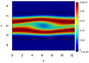
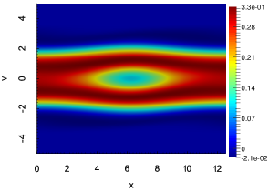
$N_{L}=50$, $[v_{a},v_{b}]=[-5,5]$
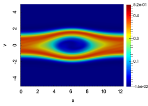
$N_{L}=100$, $[v_{a},v_{b}]=[-5,5]$
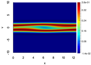
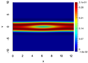
$N_{L}=100$, $[v_{a},v_{b}]=[-10,10]$

Figure 11: Two stream instability test: the plots show the distribution function $f^{e}$ in the phase space at the intermediate time $t=30$ (left panel) and the final time $t=60$ (right panel). In these calculations we use $\nu^{e}=1$, $\gamma^{e}=0.5$, $N_{F}=25$, $L=4\pi$, and three different combinations of the number of Legendre modes $N_{L}$ and the velocity range $[v_{a},v_{b}]$, which are displayed under the corresponding plots. The resolution of $f^{e}$ depends on such combinations. In particular, by comparing the plots on top and middle rows we see that the resolution of $f^{e}$ improves by increasing $N_{L}$ in a fixed velocity range. On the other hand, by comparing the plots on middle and bottom rows we see that the resolution of $f^{e}$ worsens by increasing the domain size with a fixed $N_{L}$.

where $u_{e}$ is the drift velocity. For this test case, we have chosen the following parameters: $\alpha=1/{\sqrt{8}}$, $u_{e}=1$, $\varepsilon=10^{-3}$, $k=1$. We integrate the Vlasov-Poisson system by using the time step $\Delta t=0.01$, $N_{L}=201$ Legendre modes, and $2N_{F}+1=51$ Fourier modes. The domain of integration in phase space is set to $L=4\pi$, $v_{b}=-v_{a}=5$ for all the calculations shown in Figures 5-9, while in Figure 11 we show the distribution function of electrons that is computed for three different combinations of $N_{L}$ and velocity range $[v_{a},v_{b}]$. This example was also considered with similar input parameters as in Ref. in [4], where the Vlasov equation was discretized using $N_{H}=100$ Hermite modes. The electron distribution function was inizialized by combining two drifting Maxwellians centered at two different velocities, each expanded in the Hermite basis. Since the discretization was based on the Asymmetrically Weighted Hermite basis functions [17, 29], the two Maxwellians were completely described by setting only the first mode of each expansion. The remaining modes were needed to describe the non-Maxwellian evolution of the solution. When using the Legendre-Fourier discretization proposed in this work, there is no correspondence between the first mode and the Maxwellian distribution. Thus, in order to have sufficient accuracy, the spectral expansion requires to consider all the polynomial modes from the beginning.

In Figure 5 we show the first Fourier mode of the electric field $\left|E_{1}(t)\right|$ versus time for the four combinations of $\gamma^{e}\in\{0,\,0.5\}$ and $\nu^{e}\in\{0,\,1\}$. The initial part of the dynamics is the same for the four curves and one can see the development of the two-stream instability. The slope of the numerical curves matches well the theoretical slope predicted by the linear theory, which is shown as a dashed line in the plot. When $\gamma^{e}=0$, the two curves for $\nu^{s}\in\{0,\,1\}$ stop at $t\sim 25$ (slightly prior to the end of the linear phase) because of the development of a numerical instability.

When $\gamma^{e}=0.5$ and $\nu^{e}=1$ the scheme is numerically stable and reaches the final time of the simulation, $T=200$, without problems. Instead, the case $\nu^{e}=0$ stops converging at around $t\sim 130$ because of problems related to the behavior of $f^{e}$ at the boundary (as documented below).

Figure 6 (left) shows the time evolution of the $L^{2}$ norm of the distribution function $f^{e}$ normalized with respect to initial value according to (75) the cases presented in Fig. 5. Figure 6 (right) shows a zoom around $1$. One can clearly see that the $L^{2}$ norm of $f^{e}$ grows unboundedly when $\gamma^{e}=0$, indicating that the first term on the right hand side of equation (41) provides a positive feedback that is not even compensated by the collisional term when $\nu^{e}=1$. Hence, the scheme is numerically unstable.

When $\gamma^{e}=0.5$ the scheme is numerically stable. Indeed, by applying $\gamma^{e}$ to all the moment equation, we have verified numerically that the $L^{2}$ norm of $f^{e}$ is constant in time for $\nu^{e}=0$ and damps for $\nu^{e}=1$ as predicted by Theorem $3.2$, cf. equation (47). If $\gamma^{e}$ is applied to all the Legendre modes except the first three we obtain the behavior shown in Figure 6, where a slow growth of the $L^{2}$ norm of $f^{e}$ is visible for $\nu^{e}=0$. Figure 7 shows the numerical representation of equation (41), where the time derivative is approximated by central finite differences for the case $\gamma^{e}=0.5$ and $\nu^{e}=1$. From this figure, we deduce that Theorem 3.1 and equation (41), are verified numerically to a good degree of accuracy.

The behavior of the maximum value of the distribution function on the domain boundary, $\left|f_{BC}\right|$, is shown in Fig. 8. As expected, for $\gamma^{e}=0$ the simulation is unstable and $f^{e}$ grows unbounded on the boundary. The stabilization provided by $\gamma^{e}=0.5$ is effective and limits the value of $f$ there. However, when $\nu^{e}=0$ one can see that $\left|f_{BC}\right|$ still grows sizably and becomes of order unity (i.e. of the same order of the initial distribution function) at around $t\approx 50$. Clearly this signals that the simulation is not accurate anymore. When $\nu^{e}=1$, on the other hand, $\left|f_{BC}\right|$ remains reasonably small throughout the simulation.

In Figures 9 and 10 we show the variation in time of momentum (left plot, $P(t^{\tau})-P(0)$ although $P(0)=0$ in this case) and relative variation in time of total energy (right plot, $(\mathcal{E}_{tot}(t^{\tau})-\mathcal{E}_{tot}(0))/{\mathcal{E}_{tot}(0)}$) with respect to the initial value. As for all the previous figures, the plots shown in Figure 9 are obtained by applying the penalty $\gamma^{e}$ to all the moment equations except the first three. In this case, total momentum and total energy, as well as mass which is not shown, are conserved extremely well in the simulations, as predicted by the analysis of Sections 4 and 2.4. Instead, the results of Figure 10 are obtained by applying penalty $\gamma^{e}$ to all the moment equations. In this case, the total momentum variation that is visible is of the order of magnitude of $10^{-10}$ and total energy variation is of the order of magnitude of $10^{-3}$. These results are still in accord with the analysis of Sections 4 because we know from sections 4.2 and 4.3 that both momentum and energy variation contain boundary terms that are not included in this diagnostics. It is worth noting that these boundary terms explicitly contain $\gamma^{e}$, and are zero if $\gamma^{e}=0$ in their expression. Also note that in the two-stream instability problem, momentum is symmetric and that these results show that the symmetry of the problem is not violated by the Legendre-Fourier method.

In Figure 11 we show the electron distribution function in phase space that is computed by using three different combinations of $N_{L}$, the number of Legendre modes, and velocity range $[v_{a},v_{b}]$ for $\gamma^{s}=0.5$ and $\nu^{s}=1$. In particular, the plots on top are obtained by using $N_{L}=50$ and integrating over the velocity range $[-5,5]$; the plots in the middle are obtained by using $N_{L}=100$ and the velocity range $[-5,5]$; the plots on bottom are obtained by using $N_{L}=100$ and the velocity range $[-10,10]$. The plots on the left show the distribution function at $t=30$, the plots on the right at $t=60$. The resolution of $f^{e}$ clearly depends on the combination that is chosen: it improves by increasing $N_{L}$ in a fixed velocity range and it worsen by increasing the domain size with a fixed $N_{L}$.

5.3 Ion acoustic wave

Last, we consider the evolution of an ion acoustic wave. This is a truly multiscale example, occurring on the slow time scales associated with the ions but where the electron motion concurs in defining the properties of the wave. Following [4], we initialize a perturbation in the ion distribution function at t=0

$$f^{i}(x,v,t=0)=\frac{1}{\sqrt{2\pi}\alpha_{i}}e^{-\left(\frac{v}{\sqrt{2}\alpha_{i}}\right)^{2}}\,\left[1+\varepsilon\cos\Big{(}\frac{2\pi}{L}x\Big{)}\right]$$ (77)

while the electrons are Maxwellian and unperturbed

$$f^{e}(x,v,t=0)=\frac{1}{\sqrt{2\pi}\alpha_{e}}e^{-\left(\frac{v}{\sqrt{2}\alpha_{e}}\right)^{2}}$$ (78)

Other parameters are $L=10$, $N_{L}=101$, $2N_{F}+1=51$, $\varepsilon=0.01$, $\alpha_{i}=1/135$, $\alpha_{e}=1$, $\gamma^{e}=0.5$, while $\Delta t$ and $\nu^{s}$ are varied parametrically. Although we only present results with a smaller perturbation $\varepsilon=0.01$, we have also tried larger perturbations and essentially successfully reproduced the results of Ref. [4] for $\varepsilon=0.2$.

Figure 12 shows the amplitude of the electric field for the first Fourier mode initially excited at $t=0$. Four curves are plotted, corresponding to $\Delta t\in\{0.05,\,1\}$ and $\nu^{s}\in\{0,\,0.5\}$. The initial evolution of the system is the same for all the curves and one can see some electron oscillations. However, when $\nu^{s}=0$ the simulations are corrupted by a large amount of unphysical oscillations (quite irrespective of $\Delta t$). When $\nu^{s}=0.5$, on the other hand, the ion acoustic wave signal is recovered well: the period of $|E_{1}|$ obtained from the simulations is $197$, in good agreement with the theoretical value of $201$. We note that the curves obtained with $\nu^{s}=0.5$ and $\Delta t=0.05$ and $\Delta t=1$ are virtually indistinguishable, showing the ability of our numerical scheme to step over the faster frequency in the system, the electron plasma frequency, without any sign of numerical instability. We have also performed simulations with larger $\Delta t$ (up to $\Delta t=10$, not shown). The ion acoustic wave becomes progressively less accurate but, as expected, there is no sign of numerical instabilities.

Figure 13 shows the time evolution of the $L^{2}$ norm of the distribution function normalized as in (75) for the four simulations of Fig. 12. As for the Landau damping case, when $\nu^{s}=0$ the $L^{2}$ norm of the distribution function is flat (on the scale of the plot), indicating a minimal contribution of the boundary terms in (41). When $\nu^{s}=0.5$, the $L^{2}$ norm of the distribution function decreases in time due to the dominant contribution of the collisional term.

Figure 14 shows the maximum of $\left|f\right|$ on the boundaries of the velocity space, with the same format of Fig. 12. Although $\max\left|f_{BC}\right|$ remains fairly small for all the cases, once again one can see the beneficial effect of the collisional operator: for $\nu^{s}=0.5$ it holds that $\max\left|f_{BC}\right|$ is more than an order of magnitude smaller than for $\nu^{s}=0$.

Finally, Fig. 15 shows the time evolution of the total momentum and the relative variation of the total energy for the simulations with $\nu^{s}=0.5$ and $\Delta t=0.05$ and $\Delta t=1$ (total mass is not shown since it is conserved exactly). In general, as expected, both quantities are conserved well. One can notice that the error in the total momentum is controlled by the time step, while this is not the case for the total energy.

6 Conclusions

In this paper a spectral method for the numerical solution of the Vlasov-Poisson equations of a plasma has been presented. The plasma distribution function is decomposed in Legendre polynomials applied directly on a finite domain in velocity space. The resulting set of moment equations is further discretized spatially by a Fourier decomposition (periodic boundary conditions are assumed) and in time by a fully-implicit, second order accurate Crank-Nicolson scheme. A collisional term is also considered in the discrete model to control the filamentation effect, but does not affect the conservation properties of the method. A Jacobian-Free Newton-Krylov method (with the GMRES solver for the inner linear iterations) is used to solve the discrete non-linear equations.

The most significant aspects of our work are three. First, the method is formulated in such a way that the boundary conditions in velocity space ($f^{s}=0$ at the boundary of the velocity domain) are applied in weak form. That is, they are not enforced exactly through an expansion basis obtained by a linear combination of the Legendre polynomials. Instead, the boundary conditions are satisfied approximately via an integration by parts once the Vlasov equation is projected onto the Legendre basis functions (see Sec. 2). Second, introducing a penalty on the weak form of the boundary conditions allows the formulation of the numerical scheme to be $L^{2}$-stable. Third, the numerical scheme features conservation laws for total mass, momentum and energy in weak form. The numerical experiments performed in Sec. 5 on Landau damping, two-stream instability and ion acoustic wave test cases confirm both the stability of the method and the validity of the conservation laws.

\begin{overpic}[scale={0.8}]{lin-landau-cropped-E1_all_gr2} \put(48.0,-4.0){\large{Time}} \put(-5.0,36.0){\begin{sideways}\large$\mathbf{\left|E_{1}\right|}$\end{sideways}} \end{overpic}

Figure 1: Landau damping test: first Fourier mode of the electric field versus time for the four combinations of $\gamma^{e}\in\{0,\,0.5\}$ and $\nu^{e}\in\{0,1\}$. Penalty $\gamma^{e}$ is not applied to the equations of the first three Legendre modes.

\begin{overpic}[scale={0.5}]{lin-landau-cropped-C2_all_gr2} \put(48.0,-6.0){{Time}} \put(-8.0,21.0){\begin{sideways}{$L^{2}$ norm of $f^{s}$}\end{sideways}} \end{overpic}

\begin{overpic}[scale={0.5}]{lin-landau-cropped-dC2dt_alpha05_nu1_gr2} \put(48.0,-6.0){{Time}} \put(-8.0,13.0){\begin{sideways} {Variation of $|\!|f^{s}|\!|_{L^{2}(\Omega)}$} \end{sideways}} \end{overpic}

Figure 2: Landau damping test: the left panel shows the $L2$ norm of the electron distribution function $f^{e}$, cf. (75), versus time for the four combinations of $\gamma^{e}\in\{0,\,0.5\}$ and $\nu^{e}\in\{0,1\}$. The right panel shows the time variation of the same quantity versus time as predicted by Theorem 3.1 for $\gamma^{e}=0.5$ and $\nu^{e}=1$. The time derivative is approximated by central finite differences. Penalty $\gamma^{e}$ is not applied to the equations of the first three Legendre modes.

\begin{overpic}[scale={0.8}]{lin-landau-cropped-maxfBC_all_gr2} \put(48.0,-5.0){\large{Time}} \put(-5.0,29.0){\begin{sideways} \large{max($\left|\mathbf{f^{e}_{BC}}\right|$)} \end{sideways}} \end{overpic}

Figure 3: Landau damping test: maximum value of the electron distribution function $f^{e}$ at the boundaries of the velocity range for the four combinations of $\gamma^{e}\in\{0,\,0.5\}$ and $\nu^{e}\in\{0,\,1\}$. Penalty $\gamma^{e}$ is not applied to the equations of the first three Legendre modes.

\begin{overpic}[scale={0.8}]{lin-landau-cropped-Wtot_alpha05_nu1_gr2} \put(48.0,-5.0){\large{Time}} \put(-5.0,15.0){\begin{sideways} \large{Variation of total energy} \end{sideways}} \end{overpic}

Figure 4: Landau damping test: relative variation of the total energy versus time for $\gamma^{e}=0.5$ and $\nu^{e}=1$. Penalty $\gamma^{e}$ is not applied to the equations of the first three Legendre modes.

\begin{overpic}[scale={0.5}]{two-stream-cropped-E1_all_gr2_large} \put(48.0,-6.0){{Time}} \put(-5.0,36.0){\begin{sideways}$\mathbf{\left|E_{1}\right|}$\end{sideways}} \end{overpic}

\begin{overpic}[scale={0.5}]{two-stream-cropped-E1_all_gr2_small} \put(48.0,-6.0){{Time}} \put(-5.0,36.0){\begin{sideways}$\mathbf{\left|E_{1}\right|}$\end{sideways}} \end{overpic}

Figure 5: Two-stream instability test: first Fourier mode of the electric field versus time for the four combinations of $\gamma^{e}\in\{0,\,0.5\}$ and $\nu^{e}\in\{0,1\}$. Penalty $\gamma^{e}$ is not applied to the equations of the first three Legendre modes.

\begin{overpic}[scale={0.5}]{two-stream-cropped-C2_all_gr2_large} \put(48.0,-6.0){{Time}} \put(-8.0,21.0){\begin{sideways}{$L^{2}$ norm of $f^{s}$}\end{sideways}} \end{overpic}

\begin{overpic}[scale={0.5}]{two-stream-cropped-C2_all_gr2_small} \put(48.0,-6.0){{Time}} \put(-8.0,21.0){\begin{sideways}{$L^{2}$ norm of $f^{s}$}\end{sideways}} \end{overpic}

Figure 6: Two-stream instability test: the left panel shows the $L2$ norm of the electron distribution function $f^{e}$, cf. (75), versus time for the four combinations of $\gamma^{e}\in\{0,\,0.5\}$ and $\nu^{e}\in\{0,1\}$. The right panel is a zoom around $1$. Penalty $\gamma^{e}$ is not applied to the equations of the first three Legendre modes.

\begin{overpic}[scale={0.8}]{two-stream-cropped-dC2dt_alpha05_nu1_gr2} \put(48.0,-6.0){\large{Time}} \put(-8.0,20.0){\begin{sideways} \large{Variation of $|\!|f^{s}|\!|_{L^{2}(\Omega)}$} \end{sideways}} \end{overpic}

Figure 7: Two-stream instability test: time variation of the $L2$ norm of the electron distribution function $f^{e}$ as predicted by Theorem 3.1 versus time for $\gamma^{e}=0.5$ and $\nu^{e}=1$. The time derivative is approximated by central finite differences. Penalty $\gamma^{e}$ is not applied to the equations of the first three Legendre modes.

\begin{overpic}[scale={0.8}]{two-stream-cropped-maxfBC_all_gr2} \put(48.0,-5.0){\large{Time}} \put(-5.0,29.0){\begin{sideways} \large{max($\left|\mathbf{f^{e}_{BC}}\right|$)} \end{sideways}} \end{overpic}

Figure 8: Two-stream instability test: maximum value of the electron distribution function $f^{e}$ at the boundaries of the velocity range for the four combinations of $\gamma^{e}\in\{0,\,0.5\}$ and $\nu^{e}\in\{0,\,1\}$. Penalty $\gamma^{e}$ is not applied to the equations of the first three Legendre modes.

\begin{overpic}[scale={0.5}]{two-stream-cropped-mom_alpha05_nu1_gr2} \put(48.0,-6.0){{Time}} \put(-8.0,0.0){\begin{sideways}{Variation of total momentum}\end{sideways}} \end{overpic}

\begin{overpic}[scale={0.5}]{two-stream-cropped-Wtot_alpha05_nu1_gr2} \put(48.0,-6.0){{Time}} \put(-8.0,6.0){\begin{sideways}{Variation of total energy}\end{sideways}} \end{overpic}

Figure 9: Two-stream instability test: the left panel shows the variation of momentum with respect to its initial value versus time, i.e., $P(t^{\tau})-P(0)$; the right panel shows the relative variation of energy with respect to its initial value versus time, i.e., $(\mathcal{E}_{tot}(t^{\tau})-\mathcal{E}_{tot}(0))/{\mathcal{E}_{tot}(0)}$) for $\gamma^{e}=0.5$ and $\nu^{e}=1$. Penalty $\gamma^{e}$ is not applied to the equations of the first three Legendre modes.

\begin{overpic}[scale={0.5}]{two-stream-cropped-mom_alpha05_nu1_all} \put(48.0,-6.0){{Time}} \put(-8.0,0.0){\begin{sideways}{Variation of total momentum}\end{sideways}} \end{overpic}

\begin{overpic}[scale={0.5}]{./two-stream-cropped-Wtot_alpha05_nu1_all} \put(48.0,-6.0){{Time}} \put(-8.0,6.0){\begin{sideways}{Variation of total energy}\end{sideways}} \end{overpic}

Figure 10: Two-stream instability: variation of total energy versus time by applying $\gamma^{e}$ to all modes; the collisional coefficient is $\nu=1$. Penalty $\gamma^{e}$ is applied to the equations of all Legendre modes.

\begin{overpic}[scale={0.8}]{ion-acoustic-cropped-E1_gr2_all.pdf} \put(48.0,-4.0){\large{Time}} \put(-5.0,36.0){\begin{sideways}\large$\mathbf{\left|E_{1}\right|}$\end{sideways}} \end{overpic}

Figure 12: Ion acoustic wave test: first Fourier mode of the electric field versus time for the four combinations of $\gamma^{e}\in\{0,\,0.5\}$ and $\nu^{e}\in\{0,1\}$. Penalty $\gamma^{e}$ is not applied to the equations of the first three Legendre modes.

\begin{overpic}[scale={0.8}]{ion-acoustic-cropped-C2_gr2_all.pdf} \put(48.0,-6.0){\large{Time}} \put(-8.0,24.0){\begin{sideways}\large{$L^{2}$ norm of $f^{s}$}\end{sideways}} \end{overpic}

Figure 13: Ion acoustic wave test: time variation of the $L2$ norm of the electron distribution function as predicted by Theorem 3.1 versus time for the four combinations of $\gamma^{e}\in\{0,\,0.5\}$ and $\nu^{e}\in\{0,1\}$. Penalty $\gamma^{s}$ is not applied to the equations of the first three Legendre modes.

\begin{overpic}[scale={0.8}]{ion-acoustic-cropped-maxfBC_gr2_all.pdf} \put(48.0,-5.0){\large{Time}} \put(-5.0,29.0){\begin{sideways} \large{max($\left|\mathbf{f_{BC}}\right|$)} \end{sideways}} \end{overpic}

Figure 14: Ion acoustic wave test: maximum value of the distribution function at the boundaries of the velocity range for $\gamma^{e}=0.5$ and the four combinations of $\Delta t=0.05,\,1$ and $\nu^{s}=0,0.5$. Penalty $\gamma^{s}$ is not applied to the equations of the first three Legendre modes.

\begin{overpic}[scale={0.5}]{ion-acoustic-cropped-mom_gr2_nu05.pdf} \put(48.0,-6.0){{Time}} \put(-8.0,0.0){\begin{sideways}{Variation of total momentum}\end{sideways}} \end{overpic}

\begin{overpic}[scale={0.5}]{ion-acoustic-cropped-Wtot_gr2_nu05.pdf} \put(48.0,-6.0){{Time}} \put(-8.0,6.0){\begin{sideways}{Variation of total energy}\end{sideways}} \end{overpic}

Figure 15: Ion acoustic wave test: the left panel shows the variation of momentum with respect to its initial value versus time, i.e., $P(t^{\tau})-P(0)$; the right panel shows the relative variation of energy with respect to its initial value versus time, i.e., $(\mathcal{E}_{tot}(t^{\tau})-\mathcal{E}_{tot}(0))/{\mathcal{E}_{tot}(0)}$) for $\gamma^{e}=0.5$, $\Delta t\in\{0.05,\,1\}$ and $\nu^{s}=0.5$. Penalty $\gamma^{s}$ is not applied to the equations of the first three Legendre modes.

Appendix A Legendre polynomials: recursive relations

Consider the set of Legendre polynomials $\{L_{n}(s)\}_{n=0}^{\infty}$ that are recursively defined in $[-1,1]$ by (6). The two following recursion formulas hold:

$$v\phi_{n}(v) =\sigma_{n+1}\,\phi_{n+1}(v)+\sigma_{n}\,\phi_{n-1}(v)+\overline{\sigma}\,\phi_{n}(v),$$ (79a)

$$v^{2}\phi_{n}(v) =\sigma_{n+2}\sigma_{n+1}\,\phi_{n+2}(v)+2\sigma_{n+1}\overline{\sigma}\,\phi_{n+1}(v)+\big{(}\sigma_{n+1}^{2}+\sigma_{n}^{2}+\overline{\sigma}^{2}\big{)}\,\phi_{n}(v)$$

$$\quad+2\sigma_{n}\overline{\sigma}\,\phi_{n-1}(v)+\sigma_{n}\sigma_{n-1}\,\phi_{n-2}(v),$$ (79b)

where $\sigma_{n}$ and $\overline{\sigma}$ are defined in (12). To prove (79a), note that the left-hand side term and the two right-hand side terms of the recursion formula for $n\geq 2$ can be rewritten as

$$(2n+1)sL_{n}(s) =\frac{2}{v_{b}-v_{a}}\left(v-\frac{v_{a}+v_{b}}{2}\right)\sqrt{2n+1}\,\sqrt{2n+1}\,L_{n}(s(v))=\frac{2\sqrt{2n+1}}{v_{b}-v_{a}}\left(v-\frac{v_{a}+v_{b}}{2}\right)\,\phi_{n}(v)$$

$$(n+1)L_{n+1}(s) =\frac{n+1}{\sqrt{2(n+1)+1}}\sqrt{2(n+1)+1}\,L_{n+1}(s(v))=\frac{n+1}{\sqrt{2(n+1)+1}}\phi_{n+1}(v)$$

$$nL_{n-1}(s) =\frac{n}{\sqrt{2(n-1)+1}}\sqrt{2(n-1)+1}\,L_{n-1}(s(v))=\frac{n}{\sqrt{2(n-1)+1}}\,\phi_{n-1}(v)$$

Collecting together and rearranging the three terms yields:

$$v\phi_{n}(v)=\frac{v_{b}-v_{a}}{2}\left[\,\frac{n+1}{\sqrt{(2n+3)(2n+1)}}\,\phi_{n+1}(v)+\frac{n}{\sqrt{(2n+1)(2n-1)}}\,\phi_{n-1}(v)\right]+\frac{v_{a}+v_{b}}{2}\,\phi_{n}(v),$$

which has the same form as (79a) where $\sigma_{n}$ and $\overline{\sigma}$ can be readily determined by comparison. To prove (79b) just consider $v^{2}\phi_{n}(v)=v\big{(}v\phi_{n}(v)\big{)}$ and apply (79a) twice. Moreover, a straightforward calculation yields

$$\sigma_{n}\sigma_{n,i}=\pi_{n,i}\frac{n\sqrt{2i+1}}{2n-1},$$ (80)

and in particular we have that $\sigma_{2}\sigma_{2,1}=2\sigma_{1}\sigma_{1,0}=2$.

Integrating $\phi_{n}(v)$, $v\phi_{n}(v)$, $v^{2}\phi_{n}(v)$ and using (79b)-(79b) give other three useful recurrence formulas:

$$\int_{v_{a}}^{v_{b}}\phi_{n}(v)\d v =(v_{b}-v_{a})\delta_{n,0}$$ (81a)

$$\int_{v_{a}}^{v_{b}}v\phi_{n}(v)\d v =(v_{b}-v_{a})\big{(}\sigma_{1}\delta_{n,1}+\overline{\sigma}\delta_{n,0}\big{)}$$ (81b)

$$\int_{v_{a}}^{v_{b}}v^{2}\phi_{n}(v)\d v =(v_{b}-v_{a})\Big{(}+\big{(}\sigma_{1}^{2}+\overline{\sigma}^{2}\big{)}\,\delta_{n,0}+2\sigma_{1}\overline{\sigma}\,\delta_{n,1}+\sigma_{2}\sigma_{1}\,\delta_{n,2}\Big{)}.$$ (81c)

All these three relations follows by noting that $\phi_{0}(v)=1$ and applying the orthogonality property (8). Relation (81a) is obvious. To derive (81b) and (81c) we also note that we can remove the terms containing $\delta_{n+2,0}$ and $\delta_{n+1,0}$ since $n\geq 0$. Moreover, we can substitute $n=0,1,2$ in the $\sigma$-coefficients of $\delta_{n,0}$, $\delta_{n-1,0}$, and $\delta_{n-2,0}$, and note that the effect of $\delta_{n-1,0}$ and $\delta_{n-2,0}$ is respectively equivalent to $\delta_{n,1}$ and $\delta_{n,2}$. Finally, we note that $\sigma_{0}=0$. Relation (81b) follows from

$$\int_{v_{a}}^{v_{b}}v\phi_{n}(v)\d v =\sigma_{n+1}\,\int_{v_{a}}^{v_{b}}\phi_{n+1}(v)\d v+\sigma_{n}\,\int_{v_{a}}^{v_{b}}\phi_{n-1}(v)\d v+\overline{\sigma}\,\int_{v_{a}}^{v_{b}}\phi_{n}(v)\d v,$$

$$=(v_{b}-v_{a})\big{(}\sigma_{n+1}\delta_{n+1,0}+\sigma_{n}\delta_{n-1,0}+\overline{\sigma}\delta_{n,0}\big{)}.$$

Relation (81c) follows from

$$\int_{v_{a}}^{v_{b}}v^{2}\phi_{n}(v)\d v=\sigma_{n+2}\sigma_{n+1}\,\int_{v_{a}}^{v_{b}}\phi_{n+2}(v)\d v+2\sigma_{n+1}\overline{\sigma}\,\int_{v_{a}}^{v_{b}}\phi_{n+1}(v)\d v\hskip 113.81102pt$$

$$+\big{(}\sigma_{n+1}^{2}+\sigma_{n}^{2}+\overline{\sigma}^{2}\big{)}\,\int_{v_{a}}^{v_{b}}\phi_{n}(v)\d v+2\sigma_{n}\overline{\sigma}\,\phi_{n+1}(v)\,\int_{v_{a}}^{v_{b}}\phi_{n-1}(v)\d v+\sigma_{n}\sigma_{n-1}\,\int_{v_{a}}^{v_{b}}\phi_{n-2}(v)\d v,$$

$$=(v_{b}-v_{a})\big{(}\sigma_{n+2}\sigma_{n+1}\,\delta_{n+2,0}+2\sigma_{n+1}\overline{\sigma}\,\delta_{n+1,0}+\big{(}\sigma_{n+1}^{2}+\sigma_{n}^{2}+\overline{\sigma}^{2}\big{)}\,\delta_{n,0}$$

$$\qquad+2\sigma_{n}\overline{\sigma}\,\delta_{n+1,0}+\,\delta_{n-1,0}+\sigma_{n}\sigma_{n-1}\,\delta_{n-2,0}\big{)}.$$

Appendix B Proof of (44).

The proof of equation (44) starts by applying expansion (10), Legendre orthogonality property (8), expansion (20) and Fourier orthogonality property (21):

$$\int_{0}^{L}\int_{v_{a}}^{v_{b}}\left|f^{s}(x,v,t)\right|^{2}\d vdx=\sum_{m,n=0}^{N_{L}-1}\int_{0}^{L}C^{s}_{m}(x,t)C^{s}_{n}(x,t)\int_{v_{a}}^{v_{b}}\phi_{m}(v)\phi_{n}(v)\d vdx$$

$$\qquad=(v_{b}-v_{a})\sum_{m,n=0}^{N_{L}-1}\int_{0}^{L}C^{s}_{m}(x,t)C^{s}_{n}(x,t)\delta_{m,n}dx=(v_{b}-v_{a})\sum_{n=0}^{N_{L}-1}\int_{0}^{L}\left|C^{s}_{n}(x,t)\right|^{2}dx$$

$$\qquad=(v_{b}-v_{a})\sum_{n=0}^{N_{L}-1}\sum_{k,k^{\prime}=-N_{F}}^{N_{F}}\big{(}C^{s}_{n,k}(t)\big{)}^{\dagger}C^{s}_{n,k^{\prime}}(t)\int_{0}^{L}\psi_{-k}(x)\psi_{k}(x)dx$$

$$\qquad=(v_{b}-v_{a})L\,\sum_{n=0}^{N_{L}-1}\sum_{k,k^{\prime}=-N_{F}}^{N_{F}}\big{(}C^{s}_{n,k}(t)\big{)}^{\dagger}C^{s}_{n,k^{\prime}}(t)\delta_{-k+k^{\prime},0}=(v_{b}-v_{a})L\,\sum_{n=0}^{N_{L}-1}\sum_{k=-N_{F}}^{N_{F}}\left|C^{s}_{n,k}(t)\right|^{2}.$$

Appendix C Proof of Lemma 3.1.

To prove the left-most equality in (40), we first note that:

$$L\sum_{k=-m_{k}}^{m_{k}}(\mathbf{C}^{s}_{k})^{\dagger}\Big{[}E\star\mathbbm{B}\mathbf{C}^{s}\Big{]}_{k}=L\sum_{n=0}^{N_{L}-1}\sum_{k=-m_{k}}^{m_{k}}(C^{s}_{n,k})^{\dagger}\Big{[}E\star(\mathbbm{B}\mathbf{C}^{s})_{n}\Big{]}_{k}$$ (82)

Using the definition of the discrete Fourier expansion of the electric field $E$, the Legendre coefficients $C^{s}_{n}(x,t)$, and $(\mathbbm{B}\mathbf{C}^{s})_{n}$, we obtain:

$$L\sum_{k=-m_{k}}^{m_{k}}(C^{s}_{n,k})^{\dagger}\Big{[}E\star(\mathbbm{B}\mathbf{C}^{s})_{n}\Big{]}_{k}=L\sum_{k,k^{\prime}=-m_{k}}^{m_{k}}(C^{s}_{n,k})^{\dagger}E_{k^{\prime}}\big{(}\mathbbm{B}\mathbf{C}^{s}\big{)}_{n,k-k^{\prime}}$$

$$\qquad\qquad=\sum_{k,k^{\prime},k^{\prime\prime}=-m_{k}}^{m_{k}}(C^{s}_{n,k})^{\dagger}E_{k^{\prime}}\big{(}\mathbbm{B}\mathbf{C}^{s}\big{)}_{n,k^{\prime\prime}}\,L\delta_{-k+k^{\prime}+k^{\prime\prime},0}$$

$$\qquad\qquad=\int_{0}^{L}\left(\sum_{k=-m_{k}}^{m_{k}}(C^{s}_{n,k})^{\dagger}\psi_{-k}(x)\right)\left(\sum_{k^{\prime}=-m_{k}}^{m_{k}}E_{k^{\prime}}\psi_{k^{\prime}}(x)\right)\left(\sum_{k^{\prime\prime}=-m_{k}}^{m_{k}}\big{(}\mathbbm{B}\mathbf{C}^{s}\big{)}_{n,k^{\prime\prime}}\psi_{k^{\prime\prime}}(x)\right)\,dx$$

$$\qquad\qquad=\int_{0}^{L}C^{s}_{n}(x,t)E(x,t)\big{(}\mathbbm{B}\mathbf{C}^{s}\big{)}_{n}.$$ (83)

Then, we note that:

$$\begin{array}[]{l}\displaystyle\sum_{n=0}^{N_{L}-1}C^{s}_{n}(x,t)\,(\mathbbm{B}\mathbf{C}^{s}(x,t))_{n}=\qquad\qquad\qquad\qquad\qquad\qquad\qquad\,\,\,\,\,\,\,\mbox{\big{[}use equation~{}\eqref{eq:legendre:matB:def}\big{]}}\\[17.50002pt] \end{array}$$

$$\begin{array}[]{rll}&\qquad\displaystyle=\sum_{n=0}^{N_{L}-1}\sum_{i=0}^{n-1}\sigma_{n,i}C^{s}_{n}(x,t)C^{s}_{i}(x,t)&\qquad\mbox{\big{[}use definition of $C^{s}_{i}$ from~{}\eqref{eq:legendre:decomposition}\big{]}}\\[15.00002pt] &\qquad\displaystyle=\frac{1}{v_{b}-v_{a}}\sum_{n=0}^{N_{L}-1}\sum_{i=0}^{n-1}\sigma_{n,i}C^{s}_{n}(x,t)\int_{v_{a}}^{v_{b}}f^{s}(x,v,t)\phi_{i}(v)\d v&\qquad\mbox{\big{[}use derivative formula~{}\eqref{eq:legendre:first:derivative}\big{]}}\\[15.00002pt] &\qquad\displaystyle=\frac{1}{v_{b}-v_{a}}\sum_{n=0}^{N_{L}-1}C^{s}_{n}(x,t)\int_{v_{a}}^{v_{b}}f^{s}(x,v,t)\frac{d\phi_{n}(v)}{dv}\d v&\qquad\mbox{\big{[}use again decomposition~{}\eqref{eq:legendre:decomposition}\big{]}}\\[15.00002pt] &\qquad\displaystyle=\frac{1}{v_{b}-v_{a}}\int_{v_{a}}^{v_{b}}f^{s}(x,v,t)\frac{\partial f^{s}(x,v,t)}{\partial v}\d v&\qquad\mbox{\big{[}use the definition of the derivative\big{]}}\\[15.00002pt] &\qquad\displaystyle=\frac{1}{2(v_{b}-v_{a})}\int_{v_{a}}^{v_{b}}\frac{\partial(f^{s})^{2}}{\partial v}\d v=\displaystyle\frac{1}{2}\delta_{v}\big{[}(f^{s})^{2}\big{]}_{v_{a}}^{v_{b}}\end{array}$$

Using the last relation above in (83) and tranforming back in Fourier space yield:

$$L\sum_{k=-m_{k}}^{m_{k}}(\mathbf{C}^{s}_{k})^{\dagger}\Big{[}E\star\mathbbm{B}\mathbf{C}^{s}\Big{]}_{k} =\sum_{n=0}^{N_{L}-1}\int_{0}^{L}C^{s}_{n}(x,t)E(x,t)\big{(}\mathbbm{B}\mathbf{C}^{s}\big{)}_{n}=\frac{1}{2}\int_{0}^{L}E(x,t)\delta_{v}\big{[}(f^{s}(x,v,t))^{2}\big{]}_{v_{a}}^{v_{b}}\,dx$$

$$=\frac{1}{2}L\left[E\star\delta_{v}\big{[}(f^{s}(x,v,t))^{2}\big{]}_{v_{a}}^{v_{b}}\right]_{0},$$ (84)

where $[\,\ldots\,]_{0}$ denotes the zero-th Fourier mode and which is the first equality in (40).

Applying again the definition of the discrete Fourier transform, the right-most equality in (40) is proved as follows:

$$L\sum_{k=-m_{k}}^{m_{k}}(\mathbf{C}^{s}_{k})^{\dagger}\Big{[}E\star\delta_{v}\big{[}f^{s}\bm{\phi}\big{]}_{v_{a}}^{v_{b}}\Big{]}_{k}=L\sum_{k=-m_{k}}^{m_{k}}\sum_{n=0}^{N_{L}-1}(C^{s}_{n,k})^{\dagger}\Big{[}E\star\delta_{v}\big{[}f^{s}\phi_{n}\big{]}_{v_{a}}^{v_{b}}\Big{]}_{k}$$

$$\qquad=L\sum_{n=0}^{N_{L}-1}\sum_{k,k^{\prime}=-m_{k}}^{m_{k}}(C^{s}_{n,k})^{\dagger}E_{k^{\prime}}\Big{(}\delta_{v}\big{[}f^{s}\phi_{n}\big{]}_{v_{a}}^{v_{b}}\Big{)}_{k-k^{\prime}}$$

$$\qquad=\sum_{n=0}^{N_{L}-1}\sum_{k,k^{\prime},k^{\prime\prime}=-m_{k}}^{m_{k}}(C^{s}_{n,k})^{\dagger}E_{k^{\prime}}\Big{(}\delta_{v}\big{[}f^{s}\phi_{n}\big{]}_{v_{a}}^{v_{b}}\Big{)}_{k^{\prime\prime}}\,L\delta_{-k+k^{\prime}+k^{\prime\prime},0}$$

$$\qquad=\sum_{n=0}^{N_{L}-1}\int_{0}^{L}\left(\sum_{k=-m_{k}}^{m_{k}}(C^{s}_{n,k})^{\dagger}\psi_{-k}(x)\right)\left(\sum_{k^{\prime}=-m_{k}}^{m_{k}}E_{k^{\prime}}\psi_{k^{\prime}}(x)\right)\left(\sum_{k^{\prime\prime}=-m_{k}}^{m_{k}}\Big{(}\delta_{v}\big{[}f^{s}\phi_{n}\big{]}_{v_{a}}^{v_{b}}\Big{)}_{k^{\prime\prime}}\psi_{k^{\prime\prime}}(x)\right)\,dx$$

$$\qquad=\sum_{n=0}^{N_{L}-1}\int_{0}^{L}C^{s}_{n}(x,t)E(x,t)\delta_{v}\big{[}f^{s}(x,v,t)\phi_{n}(v)\big{]}_{v_{a}}^{v_{b}}dx$$

$$\qquad=\int_{0}^{L}E(x,t)\delta_{v}\big{[}f^{s}(x,v,t)\,\sum_{n=0}^{N_{L}-1}C^{s}_{n}(x,t)\phi_{n}(v)\big{]}_{v_{a}}^{v_{b}}dx$$

$$\qquad=\int_{0}^{L}E(x,t)\delta_{v}\big{[}f^{s}(x,v,t)^{2}\big{]}_{v_{a}}^{v_{b}}dx=L\left[E\star\delta_{v}\big{[}(f^{s})^{2}\big{]}_{v_{a}}^{v_{b}}\right]_{0}.$$ (85)

The three members of (40) are real numbers since intermediate steps in the previous developments are formed by real quantities.

References

- [1] M. Abramowitz and I. Stegun. Handbook of Mathematical Functions. Dover Publications, 1965.
- [2] T. P. Armstrong, R. C. Harding, G. Knorr, and D. Montgomery. Solution of Vlasov’s equation by transform methods. In M. Rotenberg B. Alder, S. Fernbach, editor, Methods in Computational Physics. Plasma Physics, volume 9:30. Academic Press, New York, London, 1970.
- [3] C. K. Birdsall and A. B. Langdon. Plasma Physics Via Computer Simulation. Taylor & Francis, 2004.
- [4] E. Camporeale, G. L. Delzanno, B. K. Bergen, and J. D. Moulton. On the velocity space discretization for the Vlasov-Poisson system: comparison between Hermite spectral and Particle-in-Cell methods. Part 2: fully-implicit scheme. Computer Physics Communications, 198:47–58, 2016.
- [5] E. Camporeale, G. L. Delzanno, G. Lapenta, and W. Daughton. New approach for the study of linear Vlasov stability of inhomogeneous systems. Physics of Plasmas, 13:092110, 2006.
- [6] M. H. Carpenter, D. Gottlieb, and S. Abarbanel. Time-stable boundary conditions for finite-difference schemes solving hyperbolic systems: Methodology and application to high-order compact schemes. Journal of Computational Physics, 111(2):220–236, 1994.
- [7] M. H. Carpenter, J. Nordström, and D. Gottlieb. A stable and conservative interface treatment of arbitrary spatial accuracy. Journal of Computational Physics, 148(2):341–365, 1999.
- [8] C. Z. Cheng and G. Knorr. The integration of the Vlasov equation in configuration space. Journal of Computational Physics, 22(3):330–351, 1976.
- [9] J. Crank and P. Nicolson. A practical method for numerical evaluation of solutions of partial differential equations of the heat-conduction type. Mathematical Proceedings of the Cambridge Philosophical Society, 43:50–67, 1947.
- [10] L. .K. S. Daldorff, G. Tóth, T. I. Gombosi, G. Lapenta, J. Amaya, S. Markidis, and J. U. Brackbill. Two-way coupling of a global Hall magnetohydrodynamics model with a local implicit particle-in-cell model. Journal of Computational Physics, 268:236–254, 2014.
- [11] G. L. Delzanno. Multi-dimensional, fully-implicit, spectral method for the Vlasov-Maxwell equations with exact conservation laws in discrete form. Journal of Computational Physics, 301:338 – 356, 2015.
- [12] F. Engelmann, M. Feix, E. Minardi, and J. Oxenius. Nonlinear effects from Vlasov’s equation. Physics of Fluids, 6(2):266–275, 1963.
- [13] F. Filbet, E. Sonnendrücker, and P. Bertrand. Conservative numerical schemes for the Vlasov equation. Journal of Computational Physics, 172(1):166–187, 2001.
- [14] R. Glassey. The Cauchy Problem in Kinetic Theory. Society for Industrial and Applied Mathematics, 1996.
- [15] R. J. Goldston and P. H. Rutherford. Introduction to plasma physics. Plasma Physics Series. Institute of Physics Publications, 1995.
- [16] R. Hockney and J. Eastwood. Computer Simulation Using Particles. Taylor & Francis, 1988.
- [17] J. P. Holloway. Spectral velocity discretizations for the Vlasov-Maxwell equations. Transport Theory and Statistical Physics, 25(1):1–32, 1996.
- [18] A. J. Klimas. A numerical method based on the Fourier-Fourier transform approach for modeling 1-d electron plasma evolution. Journal of Computational Physics, 50(2):270–306, 1983.
- [19] D. A. Knoll and D. E. Keyes. Jacobian-free Newton-Krylov methods: a survey of approaches and applications. Journal of Computational Physics, 193(2):357–397, 2004.
- [20] H.-O. Kreiss and G. Scherer. Finite element and finite difference methods for hyperbolic partial differential equations. In C. De Boor, editor, Mathematical Aspects of Finite Elements in Partial Differential Equations, pages 202–212. Academic Press, Inc, New York, USA, 1974.
- [21] H.-O. Kreiss and G. Scherer. On the existence of energy estimates for difference approximations for hyperbolic systems. Technical report, Department of Scientific Computing, Uppsala University, Sweden, 1977.
- [22] N. F. Loureiro, A. A. Schekochihin, and A. Zocco. Fast collisionless reconnection and electron heating in strongly magnetized plasmas. Physical Review Letters, 111:025002, Jul 2013.
- [23] G Manzini, GL Delzanno, J Vencels, and S Markidis. A Legendre-Fourier spectral method with exact conservation laws for the Vlasov-Poisson system. Journal of Computational Physics, 317:82–107, 2016.
- [24] S. Markidis, P. Henri, J. Lapenta, K. Rönnmark, M. Hamrin, Z. Meliani, and E. Laure. The fluid-kinetic Particle-in-Cell method for plasma simulations. Journal of Computational Physics, 271:415–429, 2014.
- [25] K. Mattsson and J. Nordström. Summation by Parts operators for finite difference approximations of second derivatives. Journal of Computational Physics, 199(2):503–540, September 2004.
- [26] J. Nordström, K. Forsberg, C. Adamsson, and P. Eliasson. Finite volume methods, unstructured meshes and strict stability for hyperbolic problems. Applied Numerical Mathematics, 45(4):453–473, 2003.
- [27] J. T. Parker and P. J. Dellar. Fourier-Hermite spectral representation for the Vlasov-Poisson system in the weakly collisional limit. Journal of Plasma Physics, 81:305810203, 2015.
- [28] R. Sanchez and N.J. McCormick. Review of neutron transport approximations. Nuclear Science and Engineering, 80:481–535, 1982.
- [29] J. W. Schumer and J. P. Holloway. Vlasov simulations using velocity-scaled Hermite representations. Journal of Computational Physics, 144(2):626–661, 1998.
- [30] E. Sonnendrücker, J. Roche, P. Bertrand, and A. Ghizzo. The semi-lagrangian method for the numerical resolution of the Vlasov equation. Journal of Computational Physics, 149(2):201–220, 1999.
- [31] Y. Sosov. Legendre Polynomial Expansion of the electron Boltzmann Equation Applied to the Discharge in Argon. PhD thesis. University of Toledo, Spain, 2006.
- [32] B. Strand. Summation by parts for finite difference approximations for d/dx. Journal of Computational Physics, 110(1):47–67, 1994.
- [33] M. Svärd and J. Nordström. Review of summation-by-parts schemes for initial–boundary-value problems. Journal of Computational Physics, 268:17–38, 2014.
- [34] J. Vencels, G. L. Delzanno, A. Johnson, I. Bo Peng, E. Laure, and S. Markidis. Spectral solver for multi-scale plasma physics simulations with dynamically adaptive number of moments. Procedia Computer Science, 51:1148–1157, 2015. International Conference On Computational Science, {ICCS} 2015 Computational Science at the Gates of Nature.
- [35] J. Vencels, G. L. Delzanno, G. Manzini, S. Markidis, I. Bo Peng, and V. Roytershteyn. SpectralPlasmaSolver: a Hermite-Fourier spectral code for multiscale plasma simulations. Astronum, 2016. (Submitted).
- [36] S. Wollman. Existence and uniqueness theory of the Vlasov-Poisson system with application to the problem with cylindrical symmetry. Journal of Mathematical Analysis and Applications, 90(1):138–170, 1982.