Jump Events in a 3D Edwards-Anderson Spin Glass

Abstract

The statistical properties of infrequent particle displacements, greater than a certain distance, is known as jump dynamics in the context of structural glass formers. We generalize the concept of jump to the case of a spin glass, by dividing the system in small boxes, and considering infrequent cooperative spin flips in each box. Jumps defined this way share similarities with jumps in structural glasses. We perform numerical simulations for the 3D Edwards-Anderson model, and study how the properties of these jumps depend on the waiting time after a quench. Similar to the results for structural glasses, we find that while jump frequency depends strongly on time, jump duration and jump length are roughly stationary. At odds with some results reported on studies of structural glass formers, at long enough times, the rest time between jumps varies as the inverse of jump frequency. We give a possible explanation for this discrepancy. We also find that our results are qualitatively reproduced by a fully-connected trap model.

Keywords: Spin glasses

1 Introduction

Glass formers and spin glasses have been the subject of intense theoretical, experimental and numerical research in the last decades (see for instance, [1, 2, 3] and references therein). These systems present similar phenomenology (see for instance [4]), analogous techniques have been developed in both [5, 6], and their relationship has been proved [7, 8, 9]. Thus, in spite of the details about composition, structure or kind of degrees of freedom, it is common to use the word glassy to refer to any material with a dynamics qualitatively similar to that of a glass [10].

The study of glassy systems poses a series of issues, related to the impossibility to reach equilibrium below the glass transition temperature $T_{g}$. In this case, the system evolves for ever. However, the time dependence of one-time observables, like density, energy, pressure or magnetization (in a magnetic system) is quite weak and hard to appreciate. Aging effects are more clearly observed in the behavior of two-time observables, like the autocorrelation $C(t_{2},t_{1})$ and response $R(t_{2},t_{1})$ functions, which do not depend only on the time difference $t_{2}-t_{1}$ but on $t_{1}$ and $t_{2}$ (see, for example, [11, 12, 13]).

Computer simulation methods have been of great help for the study of glasses. However, this approach is limited to rather small-scale problems, in comparison with characteristic times and lengths of real systems, which may diverge below $T_{g}$. Some numerical techniques designed to avoid the effect of boundary conditions [14], or to overcome the slow dynamics [15], have been proposed. Also, special strategies that take profit of conventional processors [16] or specific hardware [17, 18] has been reported. Thanks to these advances, simulation times can be improved noticeably [19]. Nevertheless, the asymptotic regimes in the glassy phase are still far from being reached.

An alternative to sophisticated algorithms or expensive hardware is to investigate aging-to-equilibrium dynamics [20, 21], i. e., the out-of-equilibrium relaxation at a temperature above $T_{g}$. When a system is quenched from an equilibrium state at a temperature $T_{0}$ to a lower temperature $T_{F}>T_{g}$, the transition to equilibrium takes place on a time scale related to the equilibrium relaxation time $\tau(T_{F})$, which diverges at $T_{g}$. Thus, close to $T_{g}$ the relaxation is not trivial, and some aspects of glassy dynamics should be revealed for $t\ll\tau(T_{F})$. In [21], two-time correlation functions were studied in both aging-to-equilibrium and aging regimes for a simple glass former. In [20], the authors analyzed the aging-to-equilibrium dynamics for the strong glass former SiO₂.

Most of the studies about structural glass former systems focus on macroscopic or global observables. Nevertheless, in recent years microscopic actions have been analyzed [22, 23, 24, 25, 26] in structural glass formers. It has been experimentally observed that, close to a glass transition, particles spend long times moving around a position, until they jump and start moving around another position (see, for example [27], for colloids). This has motivated a lot of work on particle jumps (see [28] and references therein). Roughly speaking, jump events are particle movements greater than a certain threshold. Different definitions have been proposed, but the statistical properties of jumps do not qualitatively depend on these details. Jumps involve a small number of particles, of the order of ten. They can be related to high decorrelation regions [29], and are expected to accelerate the dynamics. Jump length is smaller than particle size [27, 28], and it slightly decreases with cooling.

The motivations for studying jumps are manifold. Jump events are not only closely related to macroscopic evolution observables like diffusivity [30] but constitute an important ingredient in the relaxation of glass formers. They provide a bridge between structure and dynamics [31], by giving a more quantitative idea of the cage effect. This is the case in [32], where, for a 2D model at low temperature, non jumping particles were more likely found in highly ordered environments. The relationship among jumps and dynamical heterogeneities has also been established [28, 29], in terms of a facilitation mechanism [33]. The statistical properties of jumps can be related to different competing theories [28]. Also, aging in glasses was analyzed in terms of jumps by monitoring the heat transfer between system and thermal bath over a short time [34].

In [22], the microscopic dynamics of SiO₂ were analyzed and related to the macroscopic dynamics. Jump statistics where studied. The authors found that the number of jumps decreases strongly with $t$, the time elapsed since the quench, reaching equilibrium at times compatible with $\tau(T_{f})$. Other properties of jumps, as average length, time duration, and surprisingly rest time between consecutive jumps did not depend on $t$. In [23], a distinction among fist hop time (the time until the first jump) and persistence. They find that first-hop time depends on the waiting time, while persistence is independent of system age. In contrast, in [35] the authors studied the distribution functions of the first-passage time, and the persistence time, and found that both quantities evolve with time.

In this work, we study some microscopic aspects of the aging-to-equilibrium and aging dynamics of the well known 3D Edwards-Anderson (EA) spin-glass model [36, 37, 38]. This model has been extensively studied in a macroscopic way, but also microscopic results have been reported [39, 40], including the existence of a backbone [41]. Here we are not interested in understanding the long-time low-temperature regime of a large-size system. We use this model as an example to study the dynamics of jumps in a spin glass. We start by generalizing the concept of jump, introduced originally for structural glass formers, to the case of a spin glass. We find that our definition of jumps shares some similarities with the one in structural glasses, particularly, it includes displacements that contribute to the relaxation of the system. We wish to analyze whether the statistical properties of jump events reported in [22] can be reproduced in a glassy system composed of spins, instead of moving particles.

For the EA model, we find that microscopic and macroscopic relaxation times behave similarly. We also find that some variables depend strongly on time while others are nearly stationary. Thus, most of the results in [22] for a structural glass former hold for this spin glass model. For instance, jump length and jump duration are roughly stationary, while the number of jumps depends strongly on $t$. On the other hand, we find that rest time between jumps, which is independent of time in [22], has an inverse relation to jump frequency for the EA model. We draw a plausible explanation for this discrepancy. Finally, we also study jumps in a infinite dimensional trap model [42], a simplified representation of glassy systems which neglects correlations among consecutive movements. Regarding the statistical properties of individual jumps, we find a strong similarity between this simple model and the 3D-EA model.

The paper is organized as follows. In Sec. 2, we describe the model and observables. In Sec. 3, we define an equilibration time based on macroscopic observables. Main results, i.e., evolution of microscopic observables, are presented in Sec. 4. In Sec. 5 we discuss our findings and future directions. In Sec. 6, draw our conclusions. In Appendix we explain the procedure to estimate the equilibration time, and show the consistency with the equilibration time for energy.

2 Model and observables

We study the Gaussian EA model in a cube with $L$ spins by side, under periodic boundary conditions, defined by the Hamiltonian:

$$H=-\sum_{\langle i,j\rangle}J_{ij}S_{i}S_{j},$$

where the indexes $i$, $j$ run from $1$ to $L^{3}$. Spin variables take values $S_{i}=\pm 1$ and the pairs $\langle i,j\rangle$ identify nearest-neighbors. The couplings are taken randomly with a Gaussian distribution with zero mean and unit variance.

Dynamics are simulated with Metropolis algorithm. That is, at each Monte Carlo (MC) step, $N=L^{3}$ spin flip trials are performed. They are accepted or rejected according to their Boltzmann weights.

For this system, $T_{g}\simeq 0.95$ [43]. To study aging-to-equilibrium, and also aging-to-non-equilibrium, we equilibrate the system at temperature $T_{0}=3$ (we have also performed runs for $T_{0}=\infty$) for $10^{5}$ MC steps. We define $t=0$ as the time at which the system is quenched to the final temperature $T_{F}=1.5,1.2,1.0$ and also $0.9$ which is below $T_{g}$. We have run 1000 samples for each temperature, for $10^{6}$ MC steps, after the quench. We have also run at least 60 samples for $10^{8}$ MC steps. We will focus on the range $10^{3}<t<10^{6}$ where most interesting phenomena takes place.

In next paragraphs, we define several microscopic observables, by dividing the full system into cubic boxes of side $l_{b}$, which contain $N_{b}=l_{b}^{3}$ spins each. Unless explicitly stated, we have worked with $L=16$ and $l_{b}=4$. Then, each box $C_{i}$ is labeled with index $i$ running from $1$ to $64$. We record the configuration every $\delta t=5$ MC steps which we will call a unit time.

We define the overlap between consecutive records of box $i$ as

$$O_{i}(t)=\frac{1}{N_{b}}\sum_{j\in C_{i}}S_{j}(t)S_{j}(t-\delta t)\,\,\,\mbox{,}$$ (1)

which we compute for $t=n\delta t$, with $n$ a positive integer. The magnetization $M_{i}$ and the energy $E_{i}$ of every box are defined as

$$M_{i}(t) = \sum_{j\in C_{i}}S_{j}(t),\;\;\;\;\;\mbox{and}$$ (2)

$$E_{i}(t) = {1\over 2}\sum_{j\in C_{i},k}J_{jk}S_{j}(t)S_{k}(t),$$ (3)

where $k$ is a nearest neighbor of $j$.

When the simulation ends, we calculate $\langle O_{i}\rangle$ and $\langle O_{i}^{2}\rangle$, for all boxes averaged in the time window $5.10^{5}$ MC $<t<10^{6}$ MC. With this, we calculate $\sigma_{i}=\sqrt{\langle O_{i}^{2}\rangle-\langle O_{i}\rangle^{2}}$. In figure 1 we show the values of $O_{i}$ and $\sigma_{i}$ averaged over small time windows of $10000$ MC steps, for a single box ($i=1$). We see that both quantities are nearly constant even for the lowest temperature $T_{F}=0.9<T_{g}$. This makes them reasonably robust parameters to study jumps.

Greater changes in the configuration of a single box are related to smaller values of the overlap between two consecutive configurations. We will say that box $i$ is jumping at time $t$ if

$$O_{i}(t)<\langle O_{i}\rangle-\gamma\,\sigma_{i}.$$ (4)

We have taken $\gamma=3$ in most of the cases, although we have also studied $\gamma=2$ and $\gamma=5$. The jump starts at $t_{i}$, where $t_{i}$ is the greatest value that verifies both $t_{i}<t$ and that Eq. (4) does not hold for $t_{i}$ (i.e. $O_{i}(t_{i})\geq\langle O_{i}\rangle-\gamma\,\sigma_{i}$). Similarly, the jump ends at $t_{f}>t$, if $t_{f}+\delta t$ is the smallest value that does not verify Eq. (4).

We define the jump frequency $\nu$, as the number of jumps per box per unit time. We measure it as a function of $t$. For each jump, we define a jump duration as $d=t_{f}-t_{i}$. We define the rest time $r$, as the time the particle waits until next jump. That is, the difference between $t_{i}$ for the next jump and $t_{f}$ for the current jump. We define the jump size $l$ using overlap values: we calculate the sum of the overlap changes over the times belonging to the jump, i.e. $l=\sum_{t_{i}<t\leq t_{f}}N_{b}-O_{i}(t)$.

We also compute some macroscopic one-time quantities as the total energy, magnetization, the number of spins that flip, and the global two-time correlation $C(t+\Delta t,t)$:

$$C(t+\Delta t,t)={1\over N}\sum_{i=1}^{N}S_{i}(t)S_{i}(t+\Delta t).$$ (5)

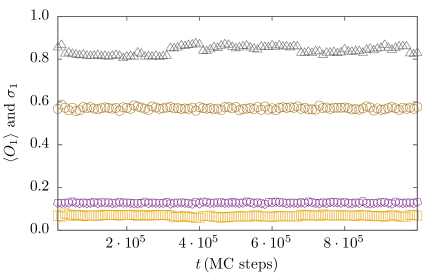
Figure 1: (Color online) $\sigma_{1}$ and $\langle O_{1}\rangle$ of a single box, as a function of $t$, for different temperatures. Black triangles: $\langle O_{1}\rangle$ for $T_{F}=0.9$. Grey circles: $\langle O_{1}\rangle$ for $T_{F}=1.5$. Orange squares: $\sigma_{1}$ for $T_{F}=0.9$. Violet pentagons: $\sigma_{1}$ for $T_{F}=1.5$.

2.1 Trap model

Many aspects of the glass transition are captured by a family of phenomenological models of traps. We will focus in the simplest case, i. e., the mean-field or fully-connected trap model introduced in [42, 44]. In this model, the system is represented by a set of energy wells of depth $E$ ($E>0$). The probability density function of wells is $\rho(E)=(1/T_{g})e^{-E/T_{g}}$. At a temperature $T$, the system may escape from its well of depth $E$ at a rate proportional to $e^{-E/T}$, and will fall in another well of depth $E^{\prime}$ chosen at random according to $\rho(E^{\prime})$. It has been shown that, in this case, a dynamical phase transition occurs at a temperature $T=T_{g}$, between a high-temperature “liquid” phase and a low-temperature “aging” phase [44]. For this fully-connected trap model, we define a jump as the escape from a trap of depth greater than a threshold $E_{t}$. Later we compare the properties of these jumps with those corresponding to the 3D-EA model. We define $\nu_{T}$ as the number of jumps per unit time; $l_{T}$ as the average energy in a well of depth greater than $E_{t}$. $d_{T}$ as the average time spent in a well with depth greater than $E_{t}$; and $r_{T}$ as the time interval among jumps.

3 Macroscopic quantities

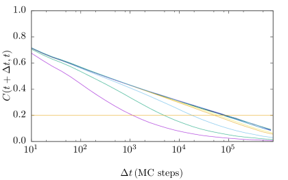
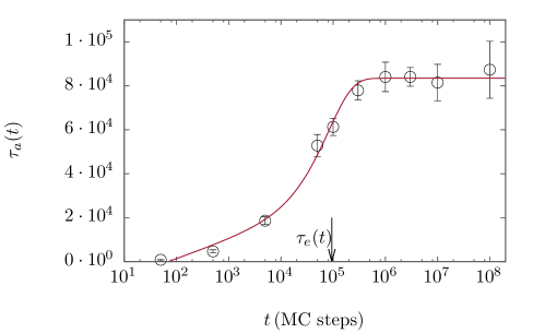
Figure 2: (Color online) Top: Global two-time correlations for $T_{F}=1.2$, and several waiting times. $t=5.,5.10,5.10^{2},5.10^{3},5.10^{4},10^{5},3.10^{5},10^{6},3.10^{6},10^{7},10^{8}$ MC steps, from left to right. The horizontal line corresponds to $C(t+\Delta t,t)=0.2$. Bottom: $\tau_{a}$ as a function of $t$ for $T_{F}=1.2$ (black circles). The (red) line corresponds to the fitting function $(C_{1}+C_{2}\log(t))e^{-t/C_{3}}+C_{4}(1-e^{-t/C_{3}})$. The arrow indicates $\tau_{e}=C_{3}$.

Our first goal is to measure the time it takes to equilibrate the system, using a macroscopic variable. Similar to [45], we find that the energy per spin, $e(t{{,T}})$ is well fitted by $e_{\infty}+A(T)t^{-b(T)}$ ($e(t,T)$ and this fit are shown in Appendix), from which a relaxation time is hard to find, so we decide to use two-times correlation functions.

It would be desirable to find $\tau_{e}^{ideal}$ such that for $t>\tau_{e}^{ideal}$, $C(t+\Delta t,t)$ does not depend on $t$. We cannot do that due to limited precision in our data. We define an auxiliary variable $\tau_{a}(t)$ such that $C(t+\tau_{a}(t),t)=K$. In our case, we choose $K=0.2$. Notice that an analogous procedure was also employed in [20, 22].

In figure 2-top, we show the two-time correlation as a function of $\Delta t$ for various values of $t$ at $T_{F}=1.2$. In figure 2-bottom, we plot $\tau_{a}(t)$ for $T_{F}=1.2$. For $T_{F}>T_{g}$, the relaxation time is then $\tau_{a}^{EQ}(T_{F})=\lim_{t\to\infty}\tau_{a}(t)$. Specific details on how we measure $\tau_{a}(t)$ are show in Appendix. The main point in this section is to get an estimate of macroscopic relaxation time.

From figure 2-bottom, we see that $\tau_{a}(t)$ grows with $t$ until it gets a constant value. To describe the growth of $\tau_{a}(t)$ at short time, and the final constant value, we have fitted $\tau_{a}(t)$ with $F(t)=(C_{1}+C_{2}\log(t))\,e^{-t/C_{3}}+C_{4}(1-e^{-t/C_{3}})$.

From this fit, we can define $\tau_{e}$, the time at which $\tau_{a}(t)$ changes from growing to constant, as $\tau_{e}=C_{3}$. Using this procedure, we were able to get $\tau_{e}$ for $T_{F}=1.5,1.35$ and $T_{F}=1.2$. Although $T_{F}=1.0>T_{g}$ we were unable to estimate $\tau_{e}$ for this temperature, since we do not have enough data for long $t$.

We have checked, for $T_{F}\geq 1.2$, that $\tau_{e}$ is a good estimate of the macroscopic equilibration time for the one-time macroscopic variables, like total energy and number of flips.

4 Mesoscopic and microscopic quantities

4.1 General characteristics of jumps

Jumps capture, at the box-size scale, the properties of the infrequent abrupt changes in energy, magnetization, and decorrelation (as described by overlap decay), which should play a key role in the relaxation process. Indeed, the dynamics become slower with time because the system gets stuck in regions of which it is increasingly hard to leave via uncorrelated spin flips. These difficulties can only be overcome with the help of cooperative movements that make up a jump; which involve only a very small fraction of time intervals. For instance: $3\%$ for $\gamma=2$, $0.4\%$ for $\gamma=3$ and $0.06\%$ for $\gamma=5$; at $T_{F}=1$. Let us remark that during a jump, not only the overlap change is large. The average absolute changes in energy and magnetization of a box are also greater (about $40\%$ and $45\%$, respectively, for $\gamma=2$; $50$ and $60\%$ for $\gamma=3$; $65$ and $70\%$ for $\gamma=5$) in a jump than in another movement.

We expect that a correlation exists between jumps and ”hard to move spins”, in the sense that the latter need special coordinated behavior of their environments to flip. To investigate this, we have studied individual flips for every spin in a single box. On the one hand, we measure the flip chance on all time steps ($f_{N}$ ); that is, the number of time steps where a given spin has flipped, divided by the whole number of time steps in the simulation. $f_{N}$ varies from about $10^{-5}$ to $10^{-1}$; i.e., there are spins (the “fast” spins) that flip $10^{4}$ times more than others (the “slow” ones). On the other hand, we measure the flip chance within a jump event ($f_{J}$); that is, the analogous to $f_{N}$ but taking into account only those time steps in which a jump is detected. As expected, $f_{N}$ is greater for fast spins than for slow ones. Nevertheless, the ratio $f_{J}/f_{N}$ has some nontrivial behavior. For fast spins, this quantity is about $1.5$, while for slow spins, it grows to about $20$. In figure 3-left we show the behavior of $f_{J}/f_{N}$ as a function of $f_{N}$ for $T_{F}=1.0$ and times up to $10^{7}$ MC steps. Note the strong correlation between jumps and slow spins, reflected in the monotonous decrease of this function. We have obtained similar behaviors for other temperatures; the lower $T_{F}$, the greater the $f_{J}/f_{N}$ ratio.

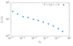
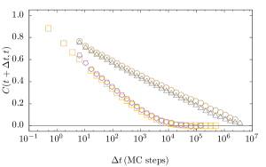
Figure 3: (Color online) Left: The ratio of flip chance on jumps to flip chance on all time steps, as a function of the latter, for $T_{F}=1$, and $\gamma=3$. Right: Two-time correlation $C(t+\Delta t,t)$ for $t=10^{6}$ MC steps. Diamonds correspond to $T_{F}=1.5$; triangles to $T_{F}=1.2$. Filled symbols show normal relaxation, while empty symbols show the constrained decay (jumping movements replaced by normal movements). Here, $\gamma=2$.

We have also checked that jumps contribute to relaxation more than normal movements, by constraining the dynamics in such way that jumps are avoided. We define a constrained dynamics as follows. If after an interval $\Delta t$, a jump is detected, the interval is repeated, i. e., time is reduced in $\Delta t$ and former configuration is loaded; otherwise the system evolves normally. In figure 3-right we plot $C(t=10^{6},t+\Delta t)$ as a function of $\Delta t$ for constrained (open symbols) and unconstrained (filled symbols) simulations, for $T_{F}=1.5$ and $T_{F}=1.2$. We define the relaxation time $\tau_{\alpha_{C}}$ for the constrained dynamics, in an analogous way to $\tau_{\alpha}$. It is worth mentioning that in the last curve we get that $\tau_{\alpha_{C}}$ is roughly twice the value of $\tau_{\alpha}$. Notice that while both simulations have run the same number of MC steps, the only difference is that jumps, which represent just $3\%$ of each boxes flips, are replaced by non-jumping movements in the constrained model. The ratio $\tau_{\alpha_{C}}/\tau_{\alpha}$ increases with $t$, and also grows on cooling; meaning that jumps become more relevant both with system age and at low temperatures.

4.2 Jump statistics

We analyze how the statistical properties of jump events evolve with time after a quench.

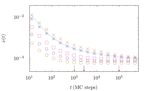
Figure 4: (Color online) Jump frequency as a function of time. Symbols correspond to $T_{0}=3$, from top to bottom, $T_{F}=0.9$, $1.0$, $1.2$, $1.35$ and $1.5$. Line with no symbols is for $T_{0}=\infty$, $T_{F}=1.0$. Arrows showing $\tau_{e}$ for $T_{F}=1.5,1.35,\mbox{and}\,1.2$ (from left to right) have been added at figure bottom. Errors are smaller than symbol size.

In figure 4, we show the jump frequency as a function of time in logarithmic scale. For $T_{F}=1.0$, we have added data for $T_{0}=\infty$, which looks qualitatively similar to the case $T_{0}=3$. This similarity holds for other values of $T_{F}$ (not shown). We see a steep decrease, consistent with the results of [22]; the slope is greater for lower temperatures. The time for which the decreasing of $\nu$ becomes negligible is compatible with macroscopic relaxation times for temperatures $T_{F}\geq 1.2$, where we are able to measure $\tau_{e}$. We have indicated these values with arrows at the bottom of figure 4, to facilitate comparison.

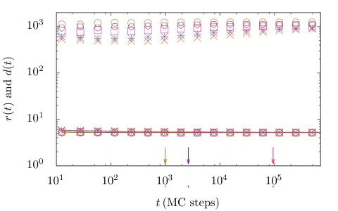
Figure 5: (Color online) Rest time (symbols) and jump duration (lines with symbols) as a function of time. For $t>10^{5}$ there is an artificial decrease of rest time, related to the finite simulation time. Symbols and colors are the same as in figure 4. Results for $T_{0}=\infty$ were avoided for the sake of clarity. Errors are smaller than symbol size.

In figure 5, we plot both jump duration $d$ and rest time $r$ against time. It is apparent that $d$ is of the order of $\delta t$, which means that most of the jump last one unit time. This is similar to the results in [22], where average jump duration is close to time step. Jump duration decreases very slowly with temperature and has no appreciable time dependence even before $\tau_{e}$. However, at odds with [22], rest time seems to evolve with $t$. This will be further discussed in next subsection.

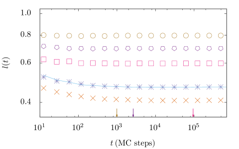
Figure 6: (Color online) Jump size as a function of time for several temperatures. Symbols and colors are the same as in figure 4. Errors are smaller than symbol size.

In figure 6, we show how the average value jump size $l$ evolves with time. Note that this quantity stabilizes well before equilibration time. Even for $T=0.9$, which is below $T_{g}$, it does for $t\sim 10^{4}$.

For the sake of completeness, in figure 7 we show the asymptotic values of $\nu$, $r$, $d$ and $l$ for all the temperatures at which we can equilibrate the system. Jump length grows with temperature and jump duration decreases, as might be expected. Jump frequency decreases with temperature and rest time grows, which may seem odd, but it can be readily understood if we notice, as shown in figure 1 that $\langle O\rangle$ decreases and $\sigma$ grows with temperature. Then, a jump at higher temperature implies the movement of a grater amount of spins.

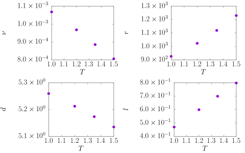
Figure 7: Asymptotic values of $\nu$, $r$, $d$ and $l$ for $T=1$, $T=1.2$, $T=1.35$ and $T=1.5$. Data was taken from results in the range $10^{5}<t<10^{6}$ for all temperatures but $T=1.0$, where data was calculated in the $10^{7}<t<10^{8}$ range. Error bars are smaller than symbol size.

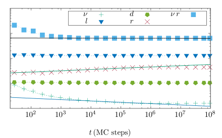
Figure 8: Symbols show results for all observables at $T=1.0$, shifted so that its comparison becomes more clear. Errors are smaller than symbol size. Dotted lines show the same results for a bigger system: $L=32$, $l_{b}=4$. Straight lines are the fit of $\nu$, $r$, and $r\nu$, as a function of $t$, using power-law forms in the range $10^{4}<t<5.10^{5}$ (for $L=16$ data). Fitted slopes for $\nu$ and $r$ are shown in table 1.

To summarize, at all temperatures, some variables change in a much more pronounced way than others. This can be better appreciated in figure 8, where we show all the previous data for $T_{F}=1.0$ in logarithmic scale. Results are shifted (multiplied by a constant) to facilitate comparison. Let us remark that while the number of jumps decreases by about one order of magnitude, other variables have negligible changes (as in [22]), with the only exception of rest time, which grows at intermediate times. Energy and magnetization jumps (not shown) also behave as jump duration or jump length, i.e. are roughly $t$ independent.

	$T_{F}$
	0.9	1.0	1.2
$s_{\nu}$	-0.082$\pm$ 0.005	-0.054$\pm$ 0.004	-0.013$\pm$ 0.002
$s_{r}$	0.080 $\pm$ 0.005	0.053 $\pm$ 0.004	0.013 $\pm$ 0.002

Table 1: Long-time effective exponents for jump frequency and rest time for $\gamma=3$ (for higher temperature, the average exponents are smaller than their errors). In all cases, data were fitted in the range $10^{4}<t<5.10^{5}$.

4.3 Issues with rest time

In Ref. [22], the authors study jumping particles, while in this work we study jumps of boxes. These quantities behave similarly, however we have found a discrepancy in the behavior of the rest time; which is roughly constant in [22]. Similarly, in [23], it is reported that the first-jump-time probability depends on time, while average persistence times does not. In contrast, in [35], it is shown that both quantities depend on the elapsed time since the quench. Since, according to our simulations (see, for example, figure 5), $r$ is time dependent, some words are in order.

We will divide our analysis into short, $t<\langle r\rangle$, intermediate, and long times, $t\gg\langle r\rangle$ (and $t>\tau_{e}$ if $T_{F}>T_{g}$). Notice that $\langle r\rangle$ depends on $T_{F}$ but also on $\gamma$.

For short enough times, i. e., for $t\ll\langle r\rangle$, most of boxes jump once or never. The results corresponding to $r(t)$ in figure 5 indicate that in this time interval ($\langle t\rangle\simeq 10^{3}$ MC steps) rest time is nearly constant. Nevertheless, the statistics is poor and biased in this case, because of the large number of boxes that cannot be considered (as they have not even done any jump). For longer times ($t\gg\langle r\rangle$), when most of jumping boxes do many jumps, it should exist some correlation between rest time and jump frequency. Since jump duration is much smaller than time between jumps, the average number of jumps per unit time, multiplied by the rest time, should be equal to the total time multiplied the number of boxes, i. e., $r\nu\simeq 1$. Thus, for long enough times, we expect that $r$ increases as $\nu$ decreases. Notice that this is what happens if figure 8, where $\nu$, $r$, $d$, $l$ but also $\nu r$ have been plotted as a function of $t$ for $T_{F}=1.0$. After a time of the order of few $\langle r\rangle$, $\nu r$ becomes constant.

To get more quantitative, we fit the data with a function $at^{s}$, for some constants $a$ and $s$ at $t$ about $10^{5}$ ($10^{4}<t<5.10^{5}$). This is an approximation for intermediate times (before equilibration, when all slopes become $0$) performed in a limited range of $t$ values. The intermediate-time ($10^{4}<t<5\,10^{5}$) effective exponents for jump frequency ($\nu(t)\sim t^{s_{\nu}}$) and rest time ($r(t)\sim t^{s_{r}}$) are opposite ($s_{\nu}\simeq-s_{r}$), within statistical error, for $T_{F}=1.0$. The same happens for other temperatures, see table 1.

For long times, we expect the relation $\nu r=1$ to hold. For $T_{F}>T_{g}$, $\nu$ and $r$ will have reached their asymptotic value. It would be interesting to study whether, for $T_{F}<T_{g}$, there is a time when $\nu$ and $r$ stop evolving. Our results for $T_{F}=0.9$, up to $10^{8}$ MC steps, suggest that this is not the case.

4.4 Sensitivity of results

In this subsection we present the results of several tests we carried out to analyze the robustness of the statistical properties of jump events.

We have checked that the outcomes for $T_{0}=3$ are similar to those for $T_{0}=\infty$. Thus, most interesting results do not depend much on $T_{0}$. Also, we found qualitatively the same results for different unit times $\delta t=2$, $5$ and $100$, though choosing smaller $\delta t$ makes the decreasing of $\nu$ more pronounced.

We have verified that doubling system size does not change the results within statistical error: see figure 8. We have measured the coherence length $\xi(t)$ as defined in [40]. The ratio of this length to system size is an important parameter in our study, since a change of regime, governed by finite size effects, is expected for $\xi(t)\simeq L$. In figure 9, we show $\xi(t)$ for $T_{F}=1.0$, $T_{F}=1.2$ and $T_{F}=1.5$. It is clear that, setting $L=16$, we are far from that regime.

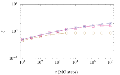
Figure 9: $\xi(t)$ for $T_{F}=1.0$, $T_{F}=1.2$ and $T_{F}=1.5$. Symbol codes are the same as in figure 4. Errors are smaller than symbol size.

Notice also that while $\xi$ is a slightly growing function of $t$, $\nu$ is strongly deceasing. The ratio $l^{3}/\xi^{3}$ is always greater than one, meaning that a jump is a pretty infrequent event in which a representative part of the spins in the box moves cooperatively.

Using an alternative definition of jumps, by changing the value of $\gamma$, also leads to the same qualitative behavior. For instance, a higher $\gamma$ (more restrictive definition, then fewer jumps) makes effective exponent of $\nu$ more negative. For example, we can compare the results for $\gamma=5$, shown in figure 10, with those for $\gamma=3$, in figure 8. Notice that, in first case, $\nu$ decreases by two orders of magnitude, while it decreases about one order of magnitude for the second. On the other hand, we can observe that the relation $\nu r=1$ does not hold about $t=10^{5}$. The reason for this behavior is that, for $\gamma=5$ the average of the rest time $\langle r\rangle$ is of the order of $10^{5}$ (while $\langle r\rangle\simeq 10^{3}$ for $\gamma=3$). Now, if we calculate the slope in the range $10^{5}<t<10^{6}$, or greater, we recover opposite slopes, see table 2.

	Time range
	$10^{4}-5\,10^{5}$	$10^{5}-10^{6}$
$s_{\nu}$	-0.097 $\pm$ 0.011	-0.081 $\pm$ 0.007
$s_{r}$	0.047 $\pm$ 0.014	0.082 $\pm$ 0.014

Table 2: Effective slopes for jump frequency and rest time for $T_{F}=1$, $\gamma=5$ and different time windows

We have also studied jump energy and jump magnetization, defined as the absolute value of the energy and magnetization differences of each box before and after the jump. These variables do not sensitively evolve with $t$. The energy and magnetization of every box also become stationary well before $\tau_{e}$. Varying $\gamma$, we found that less frequent jumps are related to greater changes in magnetization and energy.

We have explored the use of an alternative criteria of jump, with the same threshold for every box. That is, by considering that box $i$ is jumping at $t$ when $O_{i}(t)<B$, with the same constant $B$ for all boxes. We find that, since every box has a different quenched disorder, we get fast boxes jumping very frequently and slow boxes, jumping few times in the simulation time. Thus, this definition gives some unwanted results, related to the fact that rest time is severely underestimated at long $t$.

Finally, we have tried other jump criteria by defining a jump when magnetization differences overcome a certain threshold. We have found similar results to the ones presented here using this alternative criteria.

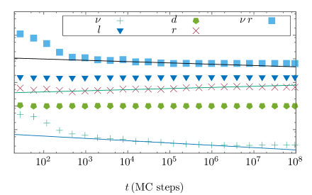
Figure 10: (Color online) Time evolution of jump properties for for $\gamma=5$. Sets of data points are shifted vertically to facilitate comparison. Let us remark that $\langle r\rangle\simeq 10^{5}$. Errors are smaller than symbol size.

The results of these tests give support to the idea that, in spite of the details of jump definition, we always get a jump frequency which depends strongly on time, but jump properties (with the exception of $r$, at intermediate times) reach stationarity much before the equilibration time.

4.5 Jumps for a trap model

Inspired by the observation that single-particle trajectories near a glass transition are characterized by long periods of localized motions followed by fast jumps, there are attempts to study glass-forming systems in terms of models of non-interacting random walkers. This is the case, for instance, of the continuous-time random walk (CTRW) model [25, 23], based on the assumption that jumps are time renewal events, i. e., that the dynamics following a jump does not depend on the history. In [46], it is argued that CTRW describes activated dynamics, but at high temperatures, or just after the quench, other relaxation mechanisms may be relevant. Interestingly, CTRW model allows for the description of an aging system, even when the movement rules do not depend on time. A key ingredient is the implicit synchronization of particles at $t=0$ [35].

Here we compare the results for the 3D-EA model with those for the fully-connected trap model defined in Sec. 2.1. Note the strong similarities between the latter and the CRTW model; both considering non-interacting particles, following each a history-independent jump dynamics (because of the infinite dimensionality, in the case of trap model).

In figure 11 we show the time evolution of the averages of jump frequency, jump size, jump duration, and rest time between jumps for the infinite dimensional trap model after a quench from $T=\infty$ to $T_{F}=1.1\;T_{g}$, and using a threshold $E_{t}=3T_{g}$ in the definition of jumps. The same qualitative behavior of these quantities and their analogs for the 3D-EA model, in figure 8, is apparent. In the case of the trap model, the average depth $l_{T}$ of a well leading to a jump, and the average time $d_{t}$ spent in it, are time independent, while rest time $r_{T}$ and jump frequency $\nu_{T}$ are inversely proportional to each other.

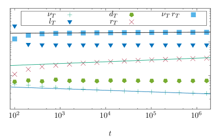
Figure 11: Time evolution of jump properties for the fully-connected trap model after a quench from $T=\infty$ to $T_{F}=1.1\;T_{g}$. The jumps are defined using a threshold $E_{t}=3T_{g}$

In order to test whether the analogy among 3D-AD and the model of traps can be extended, we have performed numerical simulations following a protocol to measure memory effects [47]. Initially, the system is quenched from equilibrium at $T_{0}=\infty$ to a temperature $T_{1}$, at which it evolves for a time $t_{1}$. Then the temperature is suddenly changed to $T_{2}$, at which the systems evolves for a time $t_{2}$. Finally, the temperature is changed back to $T_{1}$, at which the system evolves from there onward. The properties of the system following this protocol, at time $t=t_{1}+t_{2}+\Delta t$, are equivalent to that of the same system which, after the initially quench evolves always at $T_{1}$, for a time $t=t_{1}+t_{eq}+\Delta t$. This defines the equivalent time $t_{eq}$, a measure of the time at temperature $T_{1}$ for which the system evolves as much as it does for a time $t_{2}$ at temperature $T_{2}$. The equivalent time depends in principle on $T_{1},T_{2},t_{1},$ and $t_{2}$. We run simulations for several sets of these parameters, and found that regarding statistical properties of jumps, it happens that $t_{eq}\simeq t_{2}$ for both EA-3D and trap models. This is similar to the result in [48], where rejuvenation and memory numerical experiments were study for spin-glass models, and a cumulative ($t_{eq}>0$) response was found. As an example, in figure 12 we show the behavior of jump frequency following a memory-type protocol (triangles) and after simple quench (pluses), for both the 3D-EA (left) and the fully-connected trap model (right). Let us remark the similarity of the behaviors also in this case.

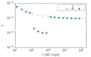
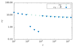
Figure 12: (Color online) Left: Jump frequency (blue triangles) for a 3D-EA model quenched from $T=\infty$ to $T_{1}=1.2$ at $t=0$ and evolving at this temperatures until $t=100$. In the interval of time $100<t<1000$ the temperature is lowered to $T_{2}=1.0$. Then, the temperature is set back to $T_{1}=1.2$ (for $1000<t<\infty$). The other data points (green pluses) correspond to jump frequency after a single initial quench at $T_{1}=1.2$. Right: Same as in left figure, for the fully-connected trap model, with $T_{1}=1.1\;T_{g}$, $T_{2}=0.5\;T_{g}$.

5 Discussion

Particle jumps in structural glasses have recently received lots of attention. They are useful in relating macroscopic observables with microscopic behavior and play an important role in system relaxation. In this work, we define jumps for spin-glass models, where the picture of escaping the cage does not apply in an obvious manner. Our definition, based on a temperature-dependent threshold for the overlap change between consecutive configurations, is inspired in the one presented in [22]. Since large overlap changes are related to large magnetization and energy changes, alternative definitions of jump using these latter quantities lead to similar results. At all studied temperatures, jumps involve a small fraction (less than $25\%$) of the spins in the box. During jumps, at $T_{F}=1.$, the average chance to move “slow” spins is about 10 times larger with respect to out-of-jumps events (figure 3-left) we observe factors of up to 100 for the slowest spins at lower temperatures (not shown). We also show that jumps contribute more than normal movements to overlap decay (figure 3-right); their relevance is greater, the lower the temperature and the longer the waiting time. Thus, as in the case of structural glasses, jump events are closely related to relaxation processes.

Simulations in the aging-to-equilibrium regime are a useful tool, because they provide glass-like dynamics in a limited time range, with well known asymptotic values. In the dynamics of relaxation towards equilibrium, we find that most one-time microscopic observables related to jumps become nearly stationary well before $\tau_{e}$. One exception is jump frequency, which is a clearly decreasing quantity for times much closer to the equilibration time. The other exception is rest time. After a few $\langle r\rangle$, $r$ evolves inversely to jump frequency, and in this sense, it is not an independent quantity. However for $t\ll\langle r\rangle$, $r$ is ill measured and we find a constant value. Then, our results are qualitatively more similar to those discussed in [35] than in [22]; the latter reporting a constant rest time for a kind of structural glass former. The strongly decreasing jump frequency, with almost $t$ insensitive jump lengths and duration, first reported in [22], is a interesting result. In that work, the authors use simulation times of the order of $\langle r\rangle$. It would be desirable to perform molecular-dynamics simulations for that system using longer simulation times, or smaller rest times (via less restrictive definition of jumps), and check whether an inverse relationship among $r$ and $\nu$ exists, after a transient of some $\langle r\rangle$’s. The asymptotic values of jump frequency, jump length, jump duration, and rest time, depend on temperature similarly as for structural glass models [25]

The strong similarity between results in figures 8 and 11, shows that even the simplest fully-connected trap model gives an aging-to-equilibrium dynamics in which the statistical properties of jumps are qualitatively the same as obtained with more detailed models. In this sense, our study gives support to the ideas underlying trap models in high dimensional spaces. By definition, the infinite dimensional trap model neglects correlations among consecutive occupied wells, and in this context, the statistical properties of jumps can be understood as follows. In equilibrium at temperature $T$ (long time average), the probability that a well of depth between $E$ and $E+\delta E$ is proportional to $\rho(E)e^{E/T}\delta E$. Then, at $t=0$, when the system is quenched to a temperature $T_{F}$ from the equilibrium state corresponding to $T=\infty$, the wells of depth between $E$ and $E+\delta E$ are occupied with a probability proportional to $\rho(E)\delta E$. This means that, initially, there will be an excess of occupied wells of low depth, in comparison with the equilibrium distribution at the working temperature. As time increases, the trap model relaxes towards equilibrium, and the high depth wells become more occupied at the expense of low depth wells; leading to a decreasing of the jump frequency. This is also the cause of the increasing of the rest time between jumps, which evolves as the inverse of $\nu_{T}$. The departure from this relation observed at short times in figure 11 appears, as mentioned above, because of the poor and biased statistics in this regime. On the other hand, since there is no correlation between consecutive jumps, the depth of the well chosen after a jump does not depend on time, neither do $d_{T}$ and $l_{T}$, which are determined by this depth.

Memory and rejuvenation numerical experiments also show that the behavior of the individual properties of jumps are qualitatively the same for the 3D-EA model as for de fully-connected trap model. Further research should be done to investigate the extent of this similarity, and the relevance of jump correlations to the dynamics of a real system.

6 Conclusion

In this work, we generalize the concept of jump, introduced in the context of glass formers [22], to the case of spin glasses. We divide the system into boxes, and define a jump as a cooperative spin flip, making the overlap function of a box to decay below a certain amount in a small time interval $\delta t$. Jumps studied this way collaborate to relaxation more than normal movements. We study the statistical properties of these jumps as a function of the waiting time $t$ after a quench, for a 3D Edwards-Anderson model of spin glass.

When this system is quenched to a temperature $T_{F}$ higher than the glass transition temperature $T_{g}\simeq 0.95$, it reaches equilibrium after a characteristic time $\tau_{e}$, which we determine numerically from the stabilization of the global two-time correlation function $C(t+\Delta t,t)$. We confirm that every statistical property of jumps becomes independent of time for $t>\tau_{e}$. At shorter times, some characteristics of jumps have a sensitive dependence on time while others do not. Jump frequency and rest time may vary on a factor of ten with negligible changes in jump length and jump duration, which reach stationarity well before $\tau_{e}$.

For $T_{F}<T_{g}$, when the equilibration time diverges, we observe that all the measured microscopic observables depend on time, in the time interval that corresponds to our simulations. However, while jump duration and jump size change very slowly, jump frequency decreases much faster. This suggests that in the glass phase the number of jumps always decreases but jumps themselves are not $t$ sensitive after a relatively short time.

These conclusions do not depend qualitatively on the chosen values of $\delta t$, system size, box size nor the details of the criteria to define a jump. In particular, if jumps are defined as a function of magnetization or energy changes instead of overlap changes, similar results are found.

The statistical properties of jumps for the 3D-EA model have qualitatively the same behavior as for the fully-connected trap model. This similarity holds also at the level of rejuvenation and memory experiments. It would be interesting to go further in this comparison by exploring correlations among jumps for the EA model, and their role in system relaxation.

Appendix: Macroscopic Relaxation Time

From $C(t+\Delta t,t)$ data, we need to estimate the value of $\tau_{a}(t)$, the value of $\Delta t$ for which $C=0.2$. Since data is subject to statistical error, it would be desirable to have an analytic expression to fit $C(t+\Delta t,t)$, such that, for a given $t$, all available information contributes to the fit. In [45], the shape of $C_{\infty}(\Delta t)\doteq\lim_{t\to\infty}C(t+\Delta t,t)$ was studied for the $\pm J$ Edwards-Anderson Model below $T_{g}$. Two alternative expressions where proposed: a power law, $C_{\infty}(\Delta t)=q_{EA}+At^{\beta}$ and a logarithmic $C_{\infty}(\Delta t)=q_{EA}+{A\over B+\log(t)}$, which performed similarly for their data. We have tried them setting $q_{EA}=0$. None of them seemed to work for our results in the whole range of times. So we have tried the simplest available approximation, $C=A+b\log(t)$. Clearly, the asymptotic form of this function is nonphysical, so we use it as a mere approximation of our data on a limited range. We have restricted our data to points where $0.1<C<0.4$ for large $t$, and smaller ranges for shorter times. This approximation gave better results (based on the comparison of goodness of fit divided by the degrees of freedom, $\chi^{2}/n$, where $n$ is the number of points used for the fit). We have also checked that $\tau_{e}(T)$ do not depend sensitively on the range of the value of $K$.

From $\tau_{a}(t)$, we have to extract $\tau_{e}(T)$. Looking at the form of the data, figure 2, we have proposed a simple way to describe it: $F(t)=(C_{1}+C_{2}\log(t))\,e^{-t/C_{3}}+C_{4}(1-e^{-t/C_{3}})$. For short times, $F(t)$ is described by the simplest growing function we could use, $C_{1}+C_{2}\log(t)$, at very long times, it goes to a constant $C_{4}$. The change of regime (from growing to constant) is given at $t=C_{3}$, so we estimate $\tau_{e}(T)=C_{3}$. This procedure also works for all investigated temperatures above $1.2$.

As mentioned in the text, $\tau_{e}(T)$ obtained this way is compatible with energy results, see figure 13.

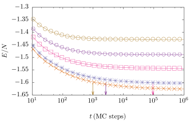
Figure 13: Points: Energy as a function of time. Line: data fit using $e+A(T)t^{b}(T)$. Errors are smaller than symbol size.

References

References

- [1] Ludovic Berthier and Giulio Biroli. Theoretical perspective on the glass transition and amorphous materials. Rev. Mod. Phys., 83:587–645, Jun 2011.
- [2] Tommaso Castellani and Andrea Cavagna. Spin-glass theory for pedestrians. Journal of Statistical Mechanics: Theory and Experiment, 2005(05):P05012, 2005.
- [3] J A Mydosh. Spin glasses: redux: an updated experimental/materials survey. Reports on Progress in Physics, 78(5):052501, 2015.
- [4] M. Tarzia and M. A. Moore. Glass phenomenology from the connection to spin glasses. Phys. Rev. E, 75:031502, Mar 2007.
- [5] Claudio Chamon, Leticia Cugliandolo, Gabriel Fabricius, José Luis Iguain, and Eric R. Weeks. From particles to spins : Eulerian formulation of supercooled liquids and glasses. PNAS, 105(40):15263–15268, 2008.
- [6] M. A. Moore and J. Yeo. Thermodynamic glass transition in finite dimensions. Phys. Rev. Lett., 96:095701, Mar 2006.
- [7] T. R. Kirkpatrick and P. G. Wolynes. Stable and metastable states in mean-field potts and structural glasses. Phys. Rev. B, 36:8552–8564, Dec 1987.
- [8] J.P. Bouchaud and M. Mézard. Self induced quenched disorder: a model for the glass transition. J. Phys. I France, 4(8):1109–1114, 1994.
- [9] E Marinari, G Parisi, and F Ritort. Replica field theory for deterministic models. ii. a non-random spin glass with glassy behaviour. Journal of Physics A: Mathematical and General, 27(23):7647, 1994.
- [10] Lectures notes in physics, complex behaviour of glassy systems, proceedings of the xiv sitges conference. In Miguel Rubí and Conrado Pérez-Vicente, editors, Lectures notes in Physics, volume 492. Springer, 1997.
- [11] Kob, W. and Barrat, J.-L. Fluctuations, response and aging dynamics in a simple glass-forming liquid out of equilibrium. Eur. Phys. J. B, 13(2):319–333, 2000.
- [12] Giorgio Parisi. Short-time aging in binary glasses. Journal of Physics A: Mathematical and General, 30(22):L765, 1997.
- [13] Enzio Andrejew and J rg Baschnagel. Aging effects in glassy polymers: a monte carlo study. Physica A: Statistical Mechanics and its Applications, 233(1):117 – 131, 1996.
- [14] Wenlong Wang, Jonathan Machta, and Helmut G. Katzgraber. Evidence against a mean-field description of short-range spin glasses revealed through thermal boundary conditions. Phys. Rev. B, 90:184412, Nov 2014.
- [15] Matteo Lulli, Giorgio Parisi, and Andrea Pelissetto. Out-of-equilibrium finite-size method for critical behavior analyses. Phys. Rev. E, 93:032126, Mar 2016.
- [16] Luis Antonio Fernández and Víctor Martín-Mayor. Testing statics-dynamics equivalence at the spin-glass transition in three dimensions. Phys. Rev. B, 91:174202, May 2015.
- [17] F. Belletti, M. Cotallo, A. Cruz, L. A. Fernandez, A. Gordillo-Guerrero, M. Guidetti, A. Maiorano, F. Mantovani, E. Marinari, V. Martin-Mayor, A. Mu oz-Sudupe, D. Navarro, G. Parisi, S. Perez-Gaviro, M. Rossi, J. J. Ruiz-Lorenzo, S. F. Schifano, D. Sciretti, A. Tarancon, R. Tripiccione, J. L. Velasco, D. Yllanes, and G. Zanier. Janus: An fpga-based system for high-performance scientific computing. Computing in Science Engineering, 11(1):48–58, Jan 2009.
- [18] M. Baity-Jesi, R.A. Ba os, A. Cruz, L.A. Fernandez, J.M. Gil-Narvion, A. Gordillo-Guerrero, D. I iguez, A. Maiorano, F. Mantovani, E. Marinari, V. Martin-Mayor, J. Monforte-Garcia, A. Mu oz Sudupe, D. Navarro, G. Parisi, S. Perez-Gaviro, M. Pivanti, F. Ricci-Tersenghi, J.J. Ruiz-Lorenzo, S.F. Schifano, B. Seoane, A. Tarancon, R. Tripiccione, and D. Yllanes. Janus ii: A new generation application-driven computer for spin-system simulations. Computer Physics Communications, 185(2):550 – 559, 2014.
- [19] F. Belletti, M. Cotallo, A. Cruz, L. A. Fernandez, A. Gordillo-Guerrero, M. Guidetti, A. Maiorano, F. Mantovani, E. Marinari, V. Martin-Mayor, A. Muñoz Sudupe, D. Navarro, G. Parisi, S. Perez-Gaviro, J. J. Ruiz-Lorenzo, S. F. Schifano, D. Sciretti, A. Tarancon, R. Tripiccione, J. L. Velasco, and D. Yllanes. Nonequilibrium spin-glass dynamics from picoseconds to a tenth of a second. Phys. Rev. Lett., 101:157201, Oct 2008.
- [20] K. Vollmayr-Lee, J. A. Roman, and J. Horbach. Aging to equilibrium dynamics of . Phys. Rev. E, 81:061203, Jun 2010.
- [21] Azita Parsaeian and Horacio E. Castillo. Equilibrium and nonequilibrium fluctuations in a glass-forming liquid. Phys. Rev. Lett., 102:055704, Feb 2009.
- [22] Katharina Vollmayr-Lee, Robin Bjorkquist, and Landon M. Chambers. Microscopic picture of aging in . Phys. Rev. Lett., 110:017801, Jan 2013.
- [23] M. Warren and J. Rottler. Atomistic mechanism of physical ageing in glassy materials. EPL (Europhysics Letters), 88(5):58005, 2009.
- [24] Mya Warren and Jörg Rottler. Microscopic view of accelerated dynamics in deformed polymer glasses. Phys. Rev. Lett., 104:205501, May 2010.
- [25] Helfferich, J., Vollmayr-Lee, K., Ziebert, F., Meyer, H., and Baschnagel, J. Glass formers display universal non-equilibrium dynamics on the level of single-particle jumps. EPL, 109(3):36004, 2015.
- [26] Anton Smessaert and Jörg Rottler. Distribution of local relaxation events in an aging three-dimensional glass: Spatiotemporal correlation and dynamical heterogeneity. Phys. Rev. E, 88:022314, Aug 2013.
- [27] Eric R Weeks and D.A Weitz. Subdiffusion and the cage effect studied near the colloidal glass transition. Chemical Physics, 284(1):361 – 367, 2002. Strange Kinetics.
- [28] Massimo Pica Ciamarra, Raffaele Pastore, and Antonio Coniglio. Particle jumps in structural glasses. Soft Matter, 12:358–366, 2016.
- [29] R. Candelier, A. Widmer-Cooper, J. K. Kummerfeld, O. Dauchot, G. Biroli, P. Harrowell, and D. R. Reichman. Spatiotemporal hierarchy of relaxation events, dynamical heterogeneities, and structural reorganization in a supercooled liquid. Phys. Rev. Lett., 105:135702, Sep 2010.
- [30] Raffaele Pastore, Antonio Coniglio, and Massimo Pica Ciamarra. From cage-jump motion to macroscopic diffusion in supercooled liquids. Soft Matter, 10:5724–5728, 2014.
- [31] Raffaele Pastore, Giuseppe Pesce, Antonio Sasso, and Massimo Pica Ciamarra. Cage size and jump precursors in glass-forming liquids: Experiment and simulations. The Journal of Physical Chemistry Letters, 8(7):1562–1568, 2017. PMID: 28301929.
- [32] R Pastore, A Coniglio, A de Candia, A Fierro, and M Pica Ciamarra. Cage-jump motion reveals universal dynamics and non-universal structural features in glass forming liquids. Journal of Statistical Mechanics: Theory and Experiment, 2016(5):054050, 2016.
- [33] Raffaele Pastore, Antonio Coniglio, and Massimo Pica Ciamarra. Spatial correlations of elementary relaxation events in glass-forming liquids. Soft Matter, 11:7214–7218, 2015.
- [34] P Sibani and H. Jeldtoft Jensen. Intermittency, aging and extremal fluctuations. Europhysics Letters (EPL), 69(4):563–569, 2005.
- [35] Nima H Siboni, Dierk Raabe, and Fathollah Varnik. Aging in amorphous solids : A study of the first passage time and persistence time distributions. Europhysics Letters (EPL), 111:48004, 2015.
- [36] S F Edwards and P W Anderson. Theory of spin glasses. Journal of Physics F: Metal Physics, 5(5):965, 1975.
- [37] W.Y Ching and D.L Huber. Monte carlo studies of the internal energy and specific heat of a classical heisenberg spin glass. Physics Letters A, 59(5):383 – 384, 1976.
- [38] K. Binder and D. Stauffer. Monte carlo simulation of a three-dimensional spin glass. Physics Letters A, 57(2):177 – 179, 1976.
- [39] Ludovic D C Jaubert, Claudio Chamon, Leticia F Cugliandolo, and Marco Picco. Growing dynamical length, scaling, and heterogeneities in the 3d edwards?anderson model. Journal of Statistical Mechanics: Theory and Experiment, 2007(05):P05001, 2007.
- [40] Markus Manssen, Alexander K. Hartmann, and A. P. Young. Nonequilibrium evolution of window overlaps in spin glasses. Phys. Rev. B, 91:104430, Mar 2015.
- [41] F. Romá and S. Risau-Gusman. Backbone structure of the edwards-anderson spin-glass model. Phys. Rev. E, 88:042105, Oct 2013.
- [42] J. P. Bouchaud. Weak ergodicity breaking and aging in disordered systems. J. Phys. I France, 2(9):1705–1713, 1992.
- [43] Helmut G. Katzgraber, Mathias Körner, and A. P. Young. Universality in three-dimensional ising spin glasses: A monte carlo study. Phys. Rev. B, 73:224432, Jun 2006.
- [44] Cécile Monthus and Jean-Philippe Bouchaud. Models of traps and glass phenomenology. Journal of Physics A: Mathematical and General, 29(14):3847, 1996.
- [45] F. Belletti, A. Cruz, L. A. Fernandez, A. Gordillo-Guerrero, M. Guidetti, A. Maiorano, F. Mantovani, E. Marinari, V. Martin-Mayor, J. Monforte, A. Mu oz Sudupe, D. Navarro, G. Parisi, S. Perez-Gaviro, J. J. Ruiz-Lorenzo, S. F. Schifano, D. Sciretti, A. Tarancon, R. Tripiccione, and D. Yllanes. An in-depth view of the microscopic dynamics of ising spin glasses at fixed temperature. Journal of Statistical Physics, 135(5):1121–1158, 2009.
- [46] Julian Helfferich. Renewal events in glass-forming liquids. The European Physical Journal E, 37(8):73, 2014.
- [47] V. Dupuis, F. Bert, J. P Bouchaud, J. Hammann, F. Ladieu, D. Parker, and E. Vincent. Aging, rejuvenation and memory phenomena in spin glasses. Pramana, 64(6):1109–1119, Jun 2005.
- [48] Andrea Maiorano, Enzo Marinari, and Federico Ricci-Tersenghi. Edwards-anderson spin glasses undergo simple cumulative aging. Phys. Rev. B, 72:104411, Sep 2005.
- [49] Tomás S. Grigera. glsim: A general library for numerical simulation. Computer Physics Communications, 182(10):2122 – 2131, 2011.