Solution of Cavity Resonance and Waveguide Scattering Problems Using the Eigenmode Projection Technique

Abstract

An eigenmode projection technique (EPT) is developed and employed to solve problems of electromagnetic resonance in closed cavities and scattering from discontinuities in guided-wave structures. The EPT invokes the eigenmodes of a canonical predefined cavity in the solution procedure and uses the expansion of these eigenmodes to solve Maxwell’s equations, in conjunction with a convenient choice of port boundary conditions. For closed cavities, resonance frequencies of arbitrary-shaped cavities are accurately determined with a robust and efficient separation method of spurious modes. For waveguide scattering problems, the EPT is combined with the generalized scattering matrix approach to solve problems involving waveguide discontinuities with arbitrary dielectric profiles. Convergence studies show stable solutions for a relatively small number of expansion modes, and the proposed method shows great robustness over conventional solvers in analyzing electromagnetic problems with inhomogeneous materials.

I Introduction

Waveguides and cavity resonators are among the oldest structures employed in the microwave regime due to the low losses of these structures at microwave frequencies. Bulky as they are, conducting waveguides and cavities remain the most robust and reliable structures in the realization of a broad spectrum of components and subsystems ranging from filters, isolators, circulators, duplexers, to particle accelerators, slotted waveguide arrays… etc. Modal solution to waveguide systems and scatterers was widely explored in the literature [1, 2, 3, 4]. Hybrid methods were also investigated, wherein modal analysis is invoked to evaluate the cutoff frequencies of dielectric-loaded waveguides [5, 6] or mode-matching-like approaches are invoked to evaluate the expansion coefficients, along with the use of a conventional numerical technique such as the finite-difference time-domain (FDTD) method [7], the finite element method (FEM) [8], and the method of moments (MoM) [9]. In this domain, several ideas were proposed to present a full wave solution to scattering problems. In [10] and [11], a Boundary Integral Method (BIM) was proposed to solve problems of cavity resonance and waveguide scattering based on the Green’s function of a spherical resonator approximated by a rational function of frequency to eliminate frequency dependence of the matrix solution. This was, however, limited to lossless, isotropic and homogeneous media, in addition to the difficulties imposed by the use of the Green’s function, the need of using suitable basis functions (such as the RWG bases) upon discretizing the surface, and the involved calculations necessary to determine the generated matrices.

In the fifties of the last century, electromagnetic field expansion inside cavities was introduced by Slater [12]. In his work, the solenoidal and irrotational cavity eigenmodes, which form a complete set, were used to represent vector fields inside microwave cavities targeting the equivalent network modeling of microwave cavities with output waveguide ports. Kurokawa [13] generalized the analysis after including irrotational modes in the magnetic field representation. Several contributions were made to fully understand the expansion and its properties [14, 15, 16]. Applications of such work were numerous in the field of microwave filters which involve cavities as high quality factor resonators, and especially in high power applications [17] and particle accelerators [18].

However, this strong theoretical framework has not been hitherto utilized to solve the sophisticated problems of scattering from arbitrary objects within the waveguide environment. Recently, the Eigenmode Projection Technique (EPT) was proposed to solve different scattering problems in guided (closed) and unguided (open) structures [19, 20, 21, 22, 23] due to its versatility, fast convergence, and straightforwardness implementation. It relies on the expansion of fields in terms of canonical (analytically known) complete set of modes to represent fields in arbitrarily shaped geometries, without the need of prior discretization of the solution domain [23]. In this paper, the proposed EPT benefits from the completeness of the eigenmodes of canonical cavities and the corresponding expansion to find a modal solution to Maxwell’s equations using mode projection, i.e., retrieve the values for the unknown fields expansion coefficients to construct the full wave solution for resonance and scattering problems in guided structures. The Generalized Scattering Matrix (GSM) approach facilitates the evaluation of the equivalent terminal voltages and currents, and the corresponding S-parameters [24] in the case of existing excitation ports. The strength of the presented technique lies in the fact that it (a) is fully capable of treating non-canonical problems using the same procedure of treating canonical cavities, (b) lends itself to integration with other techniques, such as the GSM, in a natural way, (c) is applied not only to closed problems (the scope of this work) but also to open/scattering problems, (d) lends itself inherently to problems involving bodies of revolution (BoRs), and (e) is easily extended to periodic structures [25], electrostatics [26], and even full-blown 3D geometries. For the sake of conciseness, the focus of this paper is on problems of scattering and resonance in guided-wave structures. In Section II, the formulation and the solution procedure for arbitrary electromagnetic problems using eigenmode projections is detailed. Section III covers the eigenmode solution of arbitrary shaped cavity, while Section IV explores the scattering problems inside waveguides.

II Formulation of the Eigenmode Projection Technique

Consider the arbitrarily shaped conducting cavity shown in Fig 1(a), which is generally filled with arbitrary material $\varepsilon_{r}(\mathbf{r})$ and $\mu_{r}(\mathbf{r})$, and could be excited through a number of waveguides with ports denoted by $S_{p}$. In order to solve such a problem (i.e., finding a unique full-wave solution everywhere), a canonical closed cavity that encapsulates the arbitrary-shaped cavity, with enclosing surfaces either perfect electric (PE) or perfect magnetic (PM) is chosen (as illustrated in Fig. 1(b) with dashed red color) within which the fields can be expanded in terms of known solenoidal and irrotational eigenmodes. The field expansions are used in Maxwell’s equations to solve inside the canonical cavity in presence of those materials. Subsequently, mode projections are performed. If external sources are present, parts of the fictitious cavity surface are regarded as waveguide ports (Fig. 1(c)), and appropriate boundary conditions are chosen and enforced to address the coupling to the external fields. Then, an equivalent microwave network is developed where the GSM approach is employed. Finally, the field coefficients are retrieved by solving a system of linear equations, conveniently cast in matrix form and subsequently solved using a suitable technique. A flow-chart representing the solution procedure is given in Fig. 1(d).

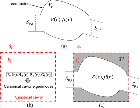
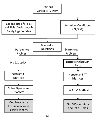
Fig. 1: (a) An arbitrary-shaped conducting cavity with arbitrary material loading and multiple waveguide ports. (b) Applying the EPT by utilizing canonical conducting cavity with known eigenmodes that are used in expanding arbitrary fields inside. (c) The wave solution of the problem in (a) is represented in terms of the canonical modes in (b). (d) Flow chart of the solution procedure of the problem.

II-A Canonical Cavity Eigenmode Expansion

Consider a canonical domain $V_{t}$ bounded by a connected surface $S_{t}$ as depicted in Fig. 1(b). The electric and magnetic fields may be cast in the form of an expansion of a known complete set of orthogonal solenoidal (divergence-free) and irrotational (curl-free) eigenmodes [12, 27] as

$$\mathbf{E}(\mathbf{r})=\sum_{n}a_{n}\mathbf{E}_{n}(\mathbf{r})+\sum_{\alpha}f_{\alpha}\mathbf{F}_{\alpha}(\mathbf{r}),$$ (1)

$$\mathbf{H}(\mathbf{r})=\sum_{n}b_{n}\mathbf{H}_{n}(\mathbf{r})+\sum_{\lambda}g_{\lambda}\mathbf{G}_{\lambda}(\mathbf{r}).$$ (2)

The solenoidal eigenmodes ($\mathbf{E}_{n}$, $\mathbf{H}_{n}$) are coupled through the curl equations

$$\nabla\times\mathbf{E}_{n}=k_{n}\mathbf{H}_{n},\,\nabla\times\mathbf{H}_{n}=k_{n}\mathbf{E}_{n},$$ (3)

and satisfy the homogeneous Helmholtz equation, viz.

$$\left(\nabla^{2}+k_{n}^{2}\right)\mathbf{E}_{n}=0,\,\left(\nabla^{2}+k_{n}^{2}\right)\mathbf{H}_{n}=0.$$ (4)

On the other hand, the irrotational eigenmodes ($\mathbf{F_{\alpha}},\,\mathbf{G_{\lambda}}$), are represented by the gradient of the scalar potentials ($\Phi_{\alpha}$, $\Psi_{\lambda}$) through

$$l_{\alpha}\mathbf{F_{\alpha}}=\nabla\Phi_{\alpha},\,w_{\lambda}\mathbf{G_{\lambda}}=\nabla\Psi_{\lambda},$$ (5)

with those scalar potentials satisfying, in turn, Helmholtz equation

$$\left(\nabla^{2}+l_{\alpha}^{2}\right)\Phi_{\alpha}=0,\,\left(\nabla^{2}+w_{\lambda}^{2}\right)\Psi_{\lambda}=0,$$ (6)

where $k_{n},\,l_{\alpha},\,w_{\lambda}$ are the wavenumbers (eigenvalues) for the solenoidal and irrotational electric and magnetic fields, respectively. Needless to say, the infinite number of modes is truncated to $N$ solenoidal modes and $M,\,K$ irrotational electric and magnetic ones, respectively. An example for the solution of the above equations is detailed in the Appendix for the encountered sample problems.

In order to use those expansions in Maxwell’s equations, expansions for $\nabla\times\mathbf{E}$, $\nabla\times\mathbf{H}$, $\nabla\cdot\mathbf{D}$ and $\nabla\cdot\mathbf{B}$ are required, but cannot be obtained by directly applying the curl and divergence operators to (1) and (2). Careful algebraic manipulations (with details in [28, 13, 27]) yield

$$\nabla\times\mathbf{E}=\sum_{n}\left(k_{n}a_{n}+\oint_{S_{t}}\mathbf{E}\times\mathbf{H}_{n}\cdot d\mathbf{s}\right)\mathbf{H}_{n}\\ +\sum_{\lambda}\left(\oint_{S_{t}}\mathbf{E}\times\mathbf{G}_{\lambda}\cdot d\mathbf{s}\right)\mathbf{G}_{\lambda}$$ (7)

$$\nabla\times\mathbf{H}=\sum_{n}\left(k_{n}b_{n}+\oint_{S_{t}}\mathbf{H}\times\mathbf{E}_{n}\cdot d\mathbf{s}\right)\mathbf{H}_{n}\\ +\sum_{\alpha}\left(\oint_{S_{t}}\mathbf{H}\times\mathbf{F}_{\alpha}\cdot d\mathbf{s}\right)\mathbf{F}_{\alpha}$$ (8)

Both the solenoidal and irrotation modes are orthogonal [28], and their amplitudes are chosen to satisfy the normalization condition, i.e.,

$$\langle\mathbf{E}_{n},\mathbf{E}_{n}\rangle_{V_{t}}=\langle\mathbf{F}_{\alpha},\mathbf{F}_{\alpha}\rangle_{V_{t}}=\langle\mathbf{H}_{n},\mathbf{H}_{n}\rangle_{V_{t}}=\langle\mathbf{G}_{\lambda},\mathbf{G}_{\lambda}\rangle_{V_{t}}=1,$$

where the term $\langle\mathbf{X},\mathbf{Y}\rangle_{V_{t}}$ denote the volumetric projection (inner product in real three-dimensional vector space) of the two vector functions $\mathbf{X}$ and $\mathbf{Y}$ and is given by,

$$\langle\mathbf{X},\mathbf{Y}\rangle_{V_{t}}=\int_{V_{t}}\mathbf{X}\cdot\mathbf{Y}dv,$$

It is worth mentioning that the expansions in (1), (2), (7), and (8) are strictly valid in the volume integral sense, i.e. the equalities are satisfied for projections (volume integrals) over arbitrary well-behaved vector functions.

II-B Problem Model and Boundary Conditions

Referring to the general problem of Fig. 1(a), the domain of volume $V_{t}$ with known eigenmodes (Fig. 1(b)) is regarded as a fictitious cavity enclosing the actual cavity $V_{c}$, which in turn may have a number of waveguide ports partially overlapping with the fictitious cavity surface $S_{t}$ as seen in Fig. 1(c). In general the treatment that will be proposed can handle cavity partially loaded with magnetic and dielectric materials. However, for the sake of simplicity, the model will be formulated only for dielectric material loading with relative permittivity $\varepsilon_{r}\left(\mathbf{r}\right)$. Beside the loading dielectric material $\varepsilon_{r}$ inside the volume $V_{c}$, the extra added space $\delta V$ (gray area in Fig. 1(c)) inside the canonical cavity is considered as a material with very high conductivity $\sigma$. Hence, the problem in Fig. 1(a) reduces to a canonical cavity loaded with a dielectric material, and the added highly conducting material that fills the space $\delta V$, in addition to the ports.

The canonical cavity walls are considered either as PE, PM, or a combination of both. In order to minimize the number of terms in the fields expansion, it is preferable to choose the fictitious cavity $V_{t}$ to conform as much as possible with the actual cavity $V_{c}$, hence minimizing the added conducting material in region $\delta V$. Therefore most of the boundaries are taken as PE, specially on boundaries coinciding with those of the actual cavity $V_{c}$. However, some boundaries may take as PM, specially those having waveguide ports through them. The ports are the excitation apertures with boundaries that are generally neither PE nor PM. But in forming the canonical cavity $V_{t}$, to make a convenient choice for the port boundaries (PE or PM) such that the cavity solenoidal and irrotational electric and magnetic eigenmodes can be analytically calculated easily. Boundary conditions for the different modes are given in the Appendix in (34) and (35), where they were used in calculating some of the modes for cylindrical and rectangular cavities employed in this paper. Either the tangential actual electric field or magnetic field vanishes on the canonical cavity surface $S_{t}$ except on surfaces of the ports $S_{p}$. Therefore, the integrals in (7) and (8) on the closed surface $S_{t}$ vanish except on the port surfaces $S_{p}$, i.e., $\oint_{S_{t}}\mathbf{E}\times\mathbf{H}_{n}\cdot d\mathbf{s}=\int_{S_{p}}\mathbf{E}\times\mathbf{H}_{n}\cdot d\mathbf{s}$.

Since these eigenmodes form a complete set, arbitrary field distributions within $V_{t}$ can be expressed by (1) and (2) under arbitrary excitation (incident fields on ports) and loading (inhomogeneous dielectric inclusions) conditions, as well as arbitrary cavity shapes $V_{c}$ as long as they are a subset of $V_{t}$.

II-C Maxwell’s Equations

Substituting the expansions (2) and (7) into Maxwell’s equation $\nabla\times\mathbf{E}=-j\omega\mu_{0}\mathbf{H}$ and performing eigenmode projection with $\mathbf{H}_{n}$ and $\mathbf{G}_{\lambda}$ and using the fact that the modes are orthonormal, yields [12, 13, 28],

$$k_{n}a_{n}+\int_{S_{p}}\left(\mathbf{E}\times\mathbf{H}_{n}\right)\cdot d\mathbf{s}=-j\omega\mu_{0}b_{n}$$ (9)

$$\int_{S_{p}}\left(\mathbf{E}\times\mathbf{G}_{\lambda}\right)\cdot d\mathbf{s}=-j\omega\mu_{0}g_{\lambda}.$$ (10)

Similarly using the expansions (1) and (8) into Maxwell’s equation $\nabla\times\mathbf{H}=j\omega\varepsilon_{0}\varepsilon_{r}(\mathbf{r})\mathbf{E}+\sigma(\mathbf{r})\mathbf{E}$ and performing eigenmode projection with $\mathbf{E}_{n}$ and $\mathbf{F}_{\alpha}$ yields,

$$k_{n}b_{n}+\int_{S_{p}}\left(\mathbf{H}\times\mathbf{E}_{n}\right)\cdot d\mathbf{s}=j\omega\varepsilon_{0}\times\\ \left[\sum_{n^{\prime}}a_{n^{\prime}}\left\langle\varepsilon_{rc}\mathbf{E}_{n},\mathbf{E}_{n^{\prime}}\right\rangle_{V}+\sum_{\alpha^{\prime}}f_{\alpha^{\prime}}\left\langle\varepsilon_{rc}\mathbf{E}_{n},\mathbf{F}_{\alpha^{\prime}}\right\rangle_{V}\right]$$ (11)

$$\int_{S_{p}}\left(\mathbf{H}\times\mathbf{F}_{\alpha}\right)\cdot d\mathbf{s}=j\omega\varepsilon_{0}\times\\ \left[\sum_{n^{\prime}}a_{n^{\prime}}\left\langle\varepsilon_{rc}\mathbf{F}_{\alpha},\mathbf{E}_{n^{\prime}}\right\rangle_{V}+\sum_{\alpha^{\prime}}f_{\alpha^{\prime}}\left\langle\varepsilon_{rc}\mathbf{F}_{\alpha},\mathbf{F}_{\alpha^{\prime}}\right\rangle_{V}\right]$$ (12)

where $\varepsilon_{rc}(\mathbf{r})=\varepsilon_{r}(\mathbf{r})-j\sigma(\mathbf{r})/\left(\omega\varepsilon_{0}\right)=\varepsilon_{r}(\mathbf{r})\left(1-j\tan\delta(\mathbf{r})\right)$ is the complex relative permitivity, which is a function of space $\mathbf{r}\in V_{t}$, written in terms of the material loss tangent. For low-loss dielectric material loading the cavity $\tan\delta\ll 1$, however for the added conducting medium in the added region $\delta V$, $\tan\delta\gg 1$, typically taken in the rest of the paper as $\tan\delta\sim 10^{4}$.

Notice that the the two Maxwell’s divergence equations $\nabla\cdot\mathbf{D}=\rho$ and $\nabla\cdot\mathbf{B}=0$ were not considered, as they can be derived from the curl equations, together with charge continuity. In fact, after some mathematical elaboration, (10) can be obtained from $\nabla\cdot\mathbf{B}=0$, whereas (12) can be derived from $\nabla\cdot\mathbf{D}=\rho$. Therefore equations (9) through (12) represent the solution of Maxwell’s equation in terms of the coefficients $a_{n}$, $b_{n}$, $f_{\alpha}$, and $g_{\lambda}$.

III Electromagnetic Cavity Resonance Analysis

A special case of the scenario depicted in Fig. 1(a) is that of a cavity resonance problem (Fig. 2(a)), viz., the cavity $V_{c}$ is not excited by external waveguides. This problem was tackled in [19], where the EPT was invoked in a procedure which involved replacing the perfectly conducting cavity surface by an equivalent surface current, expressed in terms of the fictitious canonical cavity eigenmodes. The solution resulted in a set of eigenvalues (resonance frequencies), some of which, however, were not valid resonance modes, and mostly correspond to non-zero fields in the added conducting region $\delta V$, hence named spurious modes. Identifying and separating these spurious modes required exhaustive post-processing, which was not successful in all cases in distinguishing them.

A more efficient approach is proposed here wherein a highly (but not perfectly) conducting material is used to fill in the residual part of the canonical cavity $\delta V$ (the difference between the actual cavity and canonical cavity volumes) as illustrated in Fig. 2(b), where it is simply considered as a material with very large loss tangent. It is expected that the eigenvalues (resonance frequencies) in this case will be complex and the spurious modes will be distinguished upon comparing the real and imaginary parts of the eigenvalue (or equivalently the quality factor $Q$) of the resulted modes.

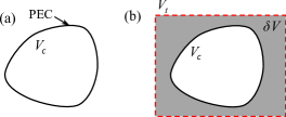
Fig. 2: (a) A conducting arbitrary-shaped cavity. (b) Employed model of the cavity as part of a conducting canonical cavity (dashed outline) partially filled with a highly conductive material (grey colored regions).

III-A Air-Filled Arbitrary-Shaped Cavity

Referring to Fig. 2(a), and assuming an air-filled cavity enclosed by a fictitious canonical cavity with the difference volume filled with a highly conductive material with a very high loss tangent $\tan\delta$ as in Fig. 2(b), the surface integrals representing coupling with port modes in (9) through (12) vanish. Hence, (10) results in $g_{\lambda}=0$, and after substituting with $b_{n}$ from (9) into (11), a set of equations in $a_{n}$ and $f_{\alpha}$ coefficients remains:

$$k_{n}^{2}a_{n}=k_{0}^{2}\left\{\sum_{n^{\prime}}a_{n^{\prime}}\left(\delta_{n^{\prime}n}-j\tan\delta\left\langle\mathbf{E}_{n},\mathbf{E}_{n^{\prime}}\right\rangle_{\delta V}\right)\right.\\ \left.-j\tan\delta\sum_{\alpha^{\prime}}f_{\alpha^{\prime}}\left\langle\mathbf{E}_{n},\mathbf{F}_{\alpha^{\prime}}\right\rangle_{\delta V}\right\}$$ (13)

$$\sum_{\alpha^{\prime}}f_{\alpha^{\prime}}\left(\delta_{\alpha^{\prime}\alpha}-j\tan\delta\left\langle\mathbf{F}_{\alpha},\mathbf{F}_{\alpha^{\prime}}\right\rangle_{\delta V}\right)=\\ -j\tan\delta\sum_{n^{\prime}}a_{n^{\prime}}\left\langle\mathbf{F}_{\alpha},\mathbf{E}_{n^{\prime}}\right\rangle_{\delta V}$$ (14)

where $\langle\cdot,\cdot\rangle_{\delta V}$ denote the volume inner product over the added conducting medium $\delta V$. Notice that (13) and (14) were simplified using the fact that modes are orthonormal, and there is no dielectric material inside the cavity, except for the added conducting one in the volume $\delta V$ which has $\varepsilon_{rc}=1-j\tan\delta$. Combining (13) and (14) and writing them in matrix form, the problem can be cast in the form of the eigenvalue problem

$$\frac{1}{k^{2}}\left[a\right]_{N\times 1}=\left[K\right]^{-1}\left(\left[U\right]_{N\times N}-j\tan\delta\left[Q^{EE}\right]_{N\times N}+\right.\\ \left.j\tan\delta\left[Q^{EF}\right]_{N\times M}\left[Z\right]_{M\times M}\left[Q^{EF}\right]_{M\times N}^{T}\right)\left[a\right]_{N\times 1},$$ (15)

$$\left[Z\right]_{M\times N}=\left[\left[Q^{FF}\right]_{M\times M}-\frac{1}{j\tan\delta}\left[U\right]_{M\times M}\right]^{-1}$$

where $\left[U\right]$ is the identity matrix, $k=2\pi f_{res}/c$ is the complex resonance wavenumber, $\left[a\right]_{N\times 1}$ is a vector of the cavity field coefficients $a_{n}$ , and the matrices $[Q^{EE}]$, $[Q^{EF}]$, and $[Q^{FF}]$ hold the values of the inner products $\langle\mathbf{E}_{n},\mathbf{E}_{n^{\prime}}\rangle_{\delta V}$, $\langle\mathbf{E}_{n},\mathbf{F}_{\alpha^{\prime}}\rangle_{\delta V}$, and $\langle\mathbf{F}_{\alpha},\mathbf{F}_{\alpha^{\prime}}\rangle_{\delta V}$, respectively, whereas $\left[K\right]^{-1}$ is inverse of a diagonal matrix $\left[K\right]$ with the diagonal elements $k_{n}^{2}$.

The eigenvalue problem in (15) is solved for the complex eigenvalues $1/k^{2}$. It is worth mentioning that although practical conductors loss tangent is frequency dependent, it is assumed that the added conductor in $\delta V$ has a constant very large loss tangent over the frequency range of interest, which would be almost identical with the practical case at microwave frequencies.

III-B Results and Convergence Study

The previous approach is first verified for the canonical case of a circular cylindrical cavity shown in inset of Fig. 3, i.e., the solution of the (actual) circular cavity of radius $b$ is obtained using the eigenmodes of another (fictitious) circular cavity of radius $a$, where $a>b$. The symmetry of the structure shown in the inset of Fig. 3 (a body-of-revolution) permits us to deal with axial symmetric modes, and implies that the axial dependence of the fields in the actual cavity will be the same that in the canonical one. Hence the axial dependence will be intentionally ignored, focusing only on transverse radial variation. Fig. 3 plots the complex eigenvalue $k$ of (15) for a case where $b=1.5$ cm and $a=2$ cm, using $30$ eigenmodes of the fictitious cavity.

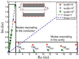
Fig. 3: Complex mode wavenumbers for circular cylinder case shown in the inset with $b$=1.5 cm, $a$=2 cm.

It is obvious from the results that the eigenvalues are directly separated into two sets: modes resonating in the conductor and modes resonating inside the cavity. The former set corresponds to spurious modes, while the latter set corresponds to the actual cavity modes. Thus, the mode separation follows in a straight-forward manner, simply by comparing the real and imaginary parts of the complex wavenumber. The actual modes are those with high real part compared to the imaginary part for high values of conductivity (i.e., high $Q$ factor). A rule-of-thumb would be that $k_{r}/k_{i}>10$ for a mode to be considered physical.

The effect of increasing the conductivity on the accuracy of the first resonance frequency is illustrated in Table I keeping the same number of eigenmodes ($N$=30) for the fictitious cavity. Also as expected, the relative error in the resonance frequency decreases as the number of eigenmodes is increased for the first resonance frequency, where for $N=$10, 20, and 30 the relative error is 4.5551%, 0.7104% and 0.0606% respectively. A final remark evident in Fig. 3 about the spurious resonance inside the added conductor is that their real and imaginary frequency parts are almost equal, a common criteria for resonances occurring inside highly conducting media.

Table I: The effect of conductivity on the accuracy of the obtained resonance frequencies

	Theoretical	$\tan\delta=10$	$\tan\delta=10^{2}$	$\tan\delta=10^{4}$
$f_{\textrm{res}}$ GHz	7.6548	6.936	7.4194	7.6502
Error %	-	9.3894 %	3.0749 %	0.0606 %

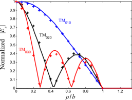
Fig. 4: Field plot versus radial distance for $\mathrm{TM_{010}}$, $\mathrm{TM_{020}}$, and $\mathrm{TM_{030}}$ modes of cavity of radius b=1.5 enclosed by canonical cavity of radius $a$ =2 cm. Crosses indicate the EPT results for $N=40$, whereas the solid line indicates the exact ones.

The solution of the eigenvalue problem results also in the eigenvectors, which represent the field coefficients of the eigenmode expansion in (1) and (2) for each resonance. Figure 4 illustrates the field plot inside the cavity using the eigenvectors (coefficients) of $\mathrm{TM_{010}}$, $\mathrm{TM_{020}}$, and $\mathrm{TM_{030}}$ modes exhibiting very good agreement with the analytical solution. It is obvious that the fields tend to zero in the conducting filling where $a<\rho<b$ smoothly, accurately, and without any oscillations. It should be emphasized, however, that the eigenmode expansion is understood in the volume-integral sense, not in a point-wise sense [23]. Thus the integrals of the field distributions are in general expected to be accurate, but this is not always the case for their point-wise evaluation. As the resonance frequencies, in the above formulation, depend on the field volume integrals, their values are also expected to be accurate as reported in the previous cases.

Second, the problem of a stepped cavity illustrated in Fig. 5 is considered, as an example of a homogeneous problem with sharp corners. The numerical solver is used to obtain reference results for TM^z resonating modes. The complex eigenvalues of stepped cavity, with dimensions $a$=2 cm, $b$=1.5 cm, $d_{in}$=3 cm, and $d$=10 cm, and $\tan\delta=10^{3}$ illustrated in Fig. 6, excellently converged to those obtained from full-wave simulations (CST Microwave Studio based on the finite element method [29]) after applying the separation of spurious using the proposed rule-of-thumb criteria, $k_{r}/k_{i}>10$, in a straightforward manner. Table II illustrates the small relative error between the resonance frequencies obtained using CST and the EPT with $N=400$ eigenmodes.

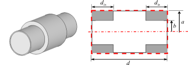
Fig. 5: Stepped cavity enclosed by cylindrical canonical cavity.

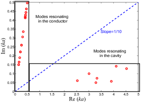
Fig. 6: Complex wavenumbers for stepped case with dimensions $a$=2 cm, $b$=1.5 cm, $d_{in}$=3 cm, and $d$=10 cm, $N=400$ with equal number of expansion modes for each direction.

Table II: The solution relative error of the first three modes for stepped cavity with loss tangent $\tan\delta=10^{3}$.

	1stRes	2ndRes	3rdRes
CST	6.058 GHz	7.2076 GHz	7.9353 GHz
EPT	6.0516 GHz	7.1805 GHz	7.8447 GHz
% Error	0.1056	0.376	1.1417

Figure 7 shows the two dimensional color map for the electric field distribution for the first two axially-symmetric $\mathrm{TM^{z}}$ modes resonating inside the cavity using the solution eigenvectors. The depicted modes exhibit very good confinement within the physical cavity with almost vanishing amplitude in the conducting residual parts of the fictitious canonical cavity.

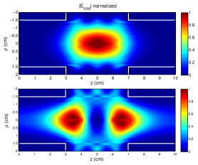
Fig. 7: Two dimensional color map for the electric field distribution for the first two axially-symmetric $\mathrm{TM^{z}}$ modes of cavity with dimensions $b$=1.5 cm, $d_{in}$=3 cm, and $d$=10 cm enclosed by canonical cavity of radius $a$=2 cm.

Third, a more practical problem is considered with cavity shape that is most common in standing wave linear accelerators (SW LINAC). In order to increase the acceleration efficiency and concentrate the electric field on the beam axis, a ‘nose cone’ is introduced on each side of the accelerating gap [30] with a geometry illustrated in Fig. 8.

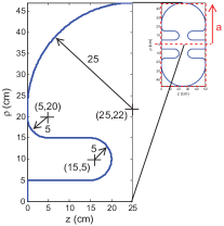
Fig. 8: Accelerating cavity with “nose cone” introduced on each side of the accelerating gap, enclosed by a cylindrical canonical cavity with radius of 47 cm and length of 50 cm.

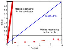
Fig. 9: Complex mode wavenumbers for the accelerator cavity described in Fig. 8.

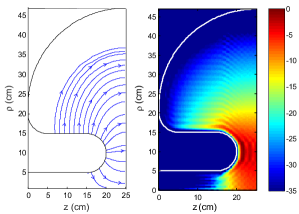
Fig. 10: Two dimensional field lines and color map distribution of the electric field of the first axially symmetric $\mathrm{TM^{z}}$ mode of cavity described in Fig. 8.

Figure 9 plots the complex eigenvalue solution $k$, using $100$ canonical eigenmodes in each of the radial and axial directions, and $\tan\delta=10^{4}$ for $\mathrm{TM^{z}}$ axially-symmetric modes. It can be observed that even with such a relatively complex structure, the physical modes are directly separable from spurious modes. The frequencies of the first two modes are 150 and 338 MHz which are only 5% and 2.5% off the results obtained using full-wave simulation (CST), respectively.

Figure 10 shows the two dimensional color map distribution of the field as well as the field lines plot for the first axially symmetric $\mathrm{TM^{z}}$ mode resonating inside the cavity using the solution eigenvectors. The results confirms the previously mentioned effect of the ‘nose cone’ in increasing the field concentration on the beam axis. Also, the mode exhibits very good confinement within the physical cavity with almost vanishing amplitude in the conducting residual parts of the fictitious canonical cavity as in previous cases.

III-C Extension to Dielectric-Loaded Cavities

The proposed EPT can be adapted in a straightforward manner to handle cavities arbitrarily loaded with dielectric materials. Consider the case shown in Fig. 11(a), where a rectangular cavity resonator loaded with a dielectric post is depicted. The resonant ${\rm TM}_{n_{1}0n_{2}}^{y}$ modes are analyzed for cavity dimensions of 20 cm $\times$ 20 cm and square dielectric post having $\varepsilon_{r}=3$ and side $h=0.5$ cm centered with respect to the cavity. Moreover, the cavity is assumed to have mixed PE/PM boundaries (the same example will be investigated later in Section IV for a waveguide scattering problem). Adaptation of the EPT to this problem is straightforward: the factor $1-j\tan\delta$ in the previous formulation will be replaced with the relative permittivity of the post. Accordingly, the resonance frequencies are obtained as discussed in Section III-A. In Table III, the resonance frequencies are calculated for the first three modes using the EPT, showing fast convergence, stability with excessive number of modes, and good agreement with results obtained using CST (error less than 0.1 % for $N=150$). Further investigation of the convergence of the field distribution is reported in the color map of the first three modes for different values of $N$ in Fig. 11(b) in the $z$ and $x$ directions. Good field convergence is achieved despite the presence of the sharp dielectric corners for 15$\times$15 eigenmodes, noting that more eigenmodes are needed for the higher order ${\rm TM}_{103}^{y}$.

The previous results have demonstrated the versatility of the EPT technique in solving any arbitrary cavity resonance problem efficiently and in a straight forward manner using a semi-analytical approach verified for canonical problems as well as other practical and general problems. Next, analysis of waveguides loaded with dielectrics is investigated.

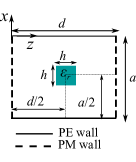
(a)

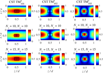
(b)

Fig. 11: (a) A rectangular cavity loaded with a dielectric square obstacle, with mixed PE/PM boundary conditions. (b) Normalized electric field $|E_{y}|$ map of the first three resonant modes obtained using CST (first row) and using the EPT for increasing $N=N_{x}\times N_{z}$ eigenmodes. The square black line denotes the location of the dielectric post.

IV Analysis of Waveguide Discontinuities

Beside the EPT capabilities of solving cavity resonance problems, the EPT lends itself to the solution of electromagnetic scattering problems from arbitrary dielectric discontinuities inside conducting waveguides [22]. In this section, scattering from dielectric objects in straight and bent waveguide sections are analyzed. For convenience, the inner product $\langle\cdot,\cdot\rangle_{S_{p}}$ will be used to denote integrals over the port surface $S_{p}$ in this section, and is not to be confused with the volume integrals in the previous section.

Table III: Resonance Frequencies for the first three ${\rm TM}_{10n}^{y}$ modes of the rectangular cavity shown in Fig. 11.

	${\rm TM}_{103}^{y}$	${\rm TM}_{103}^{y}$	${\rm TM}_{103}^{y}$
CST	6.6465	10.4599	14.5548
$N$=50	6.6595	10.4727	14.6023
$N$=150	6.6513	10.4673	14.5661
$N$=500	6.6511	10.4671	14.5648
$N$=1000	6.6511	10.4672	14.5646

IV-A Fields on Waveguide Port

The fields tangential to the ports surface $\mathbf{n}\times\mathbf{E}$ and $\mathbf{n}\times\mathbf{H}$ can be described in terms waveguide modal expansions:

$$\mathbf{n}\times\mathbf{E}=\sum_{p}V_{p}\mathbf{n}\times\mathbf{e}_{p},$$ (16)

$$\mathbf{n}\times\mathbf{H}=\sum_{p}I_{p}Z_{p}\mathbf{n}\times\mathbf{h}_{p}=\sum_{p}I_{p}\mathbf{e}_{p},$$ (17)

where $\mathbf{e}_{p}$ and $\mathbf{h}_{p}$ are the reference waveguide mode electric and magnetic fields, respectively, which are related through,

$$\mathbf{n}\times\mathbf{h_{p}}=Y_{p}\mathbf{e}_{p},$$ (18)

where $Y_{p}$ and $Z_{p}=1/Y_{p}$ are, respectively, the waveport mode admittance and impedance. In order to uniquely define the amplitudes $V_{p}$ and $I_{p}$, some normalization has to be adopted in terms of $\mathbf{e}_{p}$ and/or $\mathbf{h}_{p}$. The port transverse modal fields $\mathbf{e}_{p}$ and $\mathbf{h}_{p}$ (which correspond to the excited TE and TM waveguide modes) must be carefully normalized to take into consideration the evanescent modes, such that the GSM formulation can handle asymmetric impedance matrices properly, as in [24, 31, 32]. For simplicity, it is assumed that the field $\mathbf{e}_{p}$ is real and is normalized such that,

$$\langle\mathbf{e}_{p},\mathbf{e}_{p}\rangle_{S_{p}}=1.$$ (19)

The admittance $Y_{p}$ of the $p^{\text{th}}$ waveguide port mode is given by,

$$Y_{p}=\frac{1}{\eta_{0}}\begin{cases}{\displaystyle\frac{1}{\sqrt{1-k_{c}^{2}/k_{0}^{2}}}}&\textrm{TE}\text{ prop., }k_{0}>k_{c}\\ {\displaystyle\frac{j}{\sqrt{k_{c}^{2}/k_{0}^{2}-1}}}&\textrm{TE}\text{ Evan., }k_{0}<k_{c}\\ {\displaystyle\sqrt{1-k_{c}^{2}/k_{0}^{2}}}&\textrm{TM}\text{ prop., }k_{0}>k_{c}\\ {\displaystyle-j\sqrt{k_{c}^{2}/k_{0}^{2}-1}}&\textrm{TM}\text{ Evan., }k_{0}<k_{c}\end{cases}$$ (20)

where $k_{0}=\omega/c$ and $\eta_{0}$ are the free space wavenumber and intrinsic impedance, respectively, and $k_{c}$ is the cutoff wavenumber of the external TE/TM waveguide modes.

In contrast with cavity resonance problems, for problems with waveguide ports, not all surface port integrals that appear in (9) through (12) will vanish. To make use of the eigenmodes of some canonical cavity, however, suitable boundary conditions must be imposed on the ports. Here, PM boundaries will be assumed, i.e., $\mathbf{n}\times\mathbf{H}_{n}=\mathbf{n}\cdot\mathbf{E}_{n}=0$, and $\partial\Phi_{\alpha}/\partial n=\Psi_{\lambda}=0$. Thus, the vanishing of surface integrals in (9) gives $k_{n}a_{n}=-j\omega\mu_{0}b_{n}$ and that in (10) gives $g_{\lambda}=0$, similar to the corresponding results for closed cavity case. Using these results, the remaining port integrals are those containing the magnetic field $\mathbf{H}$ in (11) and (12) become,

$$k_{n}^{2}a_{n}-jk_{0}\eta_{0}\sum_{p}I_{p}\langle\mathbf{e}_{p},\mathbf{E}_{n}\rangle_{S_{p}}=\\ k_{0}^{2}\left[\sum_{n^{\prime}}a_{n^{\prime}}\left\langle\varepsilon_{rc}\mathbf{E}_{n},\mathbf{E}_{n^{\prime}}\right\rangle_{V_{t}}+\sum_{\alpha^{\prime}}f_{\alpha^{\prime}}\left\langle\varepsilon_{rc}\mathbf{E}_{n},\mathbf{F}_{\alpha^{\prime}}\right\rangle_{V_{t}}\right]$$ (21)

where $\langle\cdot,\cdot\rangle_{S_{p}}$ is projection on the port surface, i.e.,

$$\langle\mathbf{e}_{p},\mathbf{E}_{n}\rangle_{S_{p}}=\int_{S_{p}}\mathbf{e}_{p}\cdot\mathbf{E}_{n}ds.$$

Similarly the surface integral in (12) can be manipulated to give,

$$-j\eta_{0}\sum_{p}I_{p}\langle\mathbf{e}_{p},\mathbf{F}_{\alpha}\rangle_{S_{p}}=\\ k_{0}\left[\sum_{n^{\prime}}a_{n^{\prime}}\left\langle\varepsilon_{rc}\mathbf{F}_{\alpha},\mathbf{E}_{n^{\prime}}\right\rangle_{V_{t}}+\sum_{\alpha^{\prime}}f_{\alpha^{\prime}}\left\langle\varepsilon_{rc}\mathbf{F}_{\alpha},\mathbf{F}_{\alpha^{\prime}}\right\rangle_{V_{t}}\right]$$ (22)

Equations (21) and (22) can be cast in the following matrix form,

$$\left[\mathcal{G}\right]_{\left(M+N\right)\times\left(M+N\right)}\left[\begin{array}[]{c}\left[a\right]_{N\times 1}\\ \hdashline\left[f\right]_{M\times 1}\end{array}\right]=\\ \frac{-j\eta_{0}}{k_{0}}\left[\begin{array}[]{c}\left[Q^{Ee}\right]_{N\times P}\\ \hdashline\left[Q^{Fe}\right]_{M\times P}\end{array}\right]\left[I\right]_{P\times 1}$$ (23)

where the super-matrix $\left[\mathcal{G}\right]$ is given by,

$$\left[\mathcal{G}\right]_{\left(N+M\right)\times\left(N+M\right)}=\\ \left[\begin{array}[]{cc}\left[\varepsilon_{rc}Q^{EE}\right]_{N\times N}-\left[K\right]_{N\times N}/k_{0}^{2}&\left[\varepsilon_{rc}Q^{EF}\right]_{N\times M}\\ \hdashline\left[\varepsilon_{rc}Q^{EF}\right]_{M\times N}^{T}&\left[\varepsilon_{rc}Q^{FF}\right]_{M\times M}\end{array}\right]$$ (24)

where the sub-matrices shown in (23) and (24) are described as follows:

$\left[Q^{Ee}\right]_{N\times P}$

Matrix with entries $\langle\mathbf{E}_{n},\mathbf{e}_{p}\rangle_{S_{p}}$,

$\left[Q^{Fe}\right]_{M\times P}$

Matrix with entries $\langle\mathbf{F}_{\alpha},\mathbf{e}_{p}\rangle_{S_{p}}$,

$\left[\varepsilon_{rc}Q^{EE}\right]_{N\times N}$

Matrix with entries $\langle\varepsilon_{rc}\mathbf{E}_{n},\mathbf{E}_{n^{\prime}}\rangle_{V_{t}}$,

$\left[\varepsilon_{rc}Q^{EF}\right]_{N\times M}$

Matrix with entries $\langle\varepsilon_{rc}\mathbf{E}_{n},\mathbf{F}_{\alpha}\rangle_{V_{t}}$,

$\left[\varepsilon_{rc}Q^{FF}\right]_{M\times M}$

Matrix with entries $\langle\varepsilon_{rc}\mathbf{F}_{\alpha^{\prime}},\mathbf{F}_{\alpha}\rangle_{V_{t}}$.

Equation (23) can be solved by inverting the matrix $\mathcal{G}$ given by (24) to get the coefficients $a_{n}$ and $f_{\alpha}$ in term of the ports excitation "current" amplitudes $I_{p}$.

IV-B Matching the Port and Cavity Fields

To determine the scattered port fields, the next step would be to match the external (port) and internal (cavity) fields, such that

$$\sum_{p}V_{p}\mathbf{n}\times\mathbf{e}_{p}=\mathbf{n}\times\mathbf{E},\qquad\text{on }S_{p}$$ (25)

By projecting both sides of the equation on the port modal field $\mathbf{h}_{p^{\prime}}$, one gets,

$$\sum_{p}V_{p}\langle\mathbf{n}\times\mathbf{e}_{p},\mathbf{h}_{p^{\prime}}\rangle_{S_{p}}=\langle\mathbf{n}\times\mathbf{E},\mathbf{h}_{p^{\prime}}\rangle_{S_{p}}$$ (26)

Due to the nature of the eigenmode expansions, the total cavity field $\mathbf{E}$ may exhibit a discontinuity at the boundaries of the expansion domain, viz. the cavity, even though this field is expanded in terms of piecewise continuously differentiable eigenmodes within $V_{t}$. This mathematical artifact brings about an overshoot in the field at the boundary; a phenomenon that resembles Gibbs phenomenon in Fourier series expansions [33], for example. Consequently, the point-wise matching of fields cannot be rigorously enforced. Therefore the expansion (1) cannot be strictly used except in the volume integral forms, however after some manipulation [23], it can be shown to be valid substitution in the surface integral in Eq. (26) under the condition of considering the port boundaries as PM when calculating the canonical cavity solenoidal and irrotational modes. When the waveport modes orthogonality and normalization condition in (19) are applied on equation (26), it gives $V_{p}$ in terms of the coefficients $a_{n}$ and $f_{\alpha}$,

$$V_{p}=\sum_{n}a_{n}\langle\mathbf{e}_{p^{\prime}},\mathbf{E}_{n}\rangle_{S_{p}}+\sum_{\alpha}f_{\alpha}\langle\mathbf{e}_{p^{\prime}},\mathbf{F}_{\alpha}\rangle_{S_{p}}.$$ (27)

Solving equation (23) for the vector containing the coefficients $a_{n}$ and $f_{\alpha}$, and substituting in (27), we get the Z-matrix representation,

$$\left[V\right]_{P\times 1}=\left[Z\right]_{P\times P}\left[I\right]_{P\times 1},$$ (28)

where the impedance matrix $\left[Z\right]_{P\times P}$ is given by,

$$\left[Z\right]_{P\times P}=\frac{-j\eta_{0}}{k_{0}}\left[\begin{array}[]{cc}\left[Q^{Ee}\right]_{P\times N}^{T}&\left[Q^{Fe}\right]_{P\times M}^{T}\end{array}\right]\times\\ \left[\mathcal{G}\right]_{\left(N+M\right)\times\left(N+M\right)}^{-1}\left[\begin{array}[]{c}\left[Q^{Ee}\right]_{N\times P}\\ \hdashline\left[Q^{Fe}\right]_{M\times P}\end{array}\right]$$ (29)

purely imaginary for lossless case where $\varepsilon_{rc}$ is real.

Now in order to get the scattering parameters $\left[S\right]$, the following relation for the incident and scattered wave amplitudes will be used.

$$V_{p}=V_{p}^{+}+V_{p}^{-},\qquad I_{p}Z_{p}=V_{p}^{+}-V_{p}^{-}$$

$$\left[V_{p}^{-}\right]=\left[S\right]\left[V_{p}^{+}\right]$$

$$[S]=\left(\left[Z\right]\left[\Upsilon\right]-\left[U\right]\right)\left(\left[Z\right]\left[\Upsilon\right]+\left[U\right]\right)^{-1},$$ (30)

where $\left[\Upsilon\right]_{P\times P}$ is a diagonal matrix with diagonal elements $Y_{p}$. The generalized scattering matrix GSM can be obtained from the normalized impedance matrix $\left[\bar{Z}\right]$,

$$\left[\bar{Z}\right]=\left[\sqrt{\Upsilon}\right]\left[Z\right]\left[\sqrt{\Upsilon}\right],$$

$$\left[S^{g}\right]=\left(\left[\bar{Z}\right]-\left[U\right]\right)\left(\left[\bar{Z}\right]+\left[U\right]\right)^{-1}$$ (31)

where $\left[\sqrt{\Upsilon}\right]_{P\times P}$ is a diagonal matrix with diagonal elements $+\sqrt{Y_{p}}$ . It can be easily shown that the relation between $\left[S\right]$ (30) and $\left[S^{g}\right]$ (31) is,

$$\left[S^{g}\right]=\left[\sqrt{\Upsilon}\right]\left[S\right]\left[\sqrt{\Upsilon}\right]^{-1}$$ (32)

It should be mentioned that there will ambiguity in calculating $\left[\sqrt{\Upsilon}\right]$ in (31) and (32) due to the evanescent modes in the lossless waveguide.

IV-C Dielectric Loaded Waveguides 2D Examples

The previous procedure is used here to solve an example of a $90^{\circ}$ rectangular waveguide bend shown in Fig. 12 having dimensions $a=2$ cm and $d$$=2$ cm, partially loaded with four circular posts with $\varepsilon_{r}=3$, $\mu_{r}=1$, $\tan\delta=0.01$ and of radii $r=a/8$, and height of $b$ = 1 cm which is equal to that of the waveguide in the y-direction. The input port is excited with the $\textrm{TE}_{10}^{y}$ mode, and both ports are modeled as a PM surfaces. The problem becomes y-invariant according to these particular choices, i.e., a 2D problem (see Appendix for details of eigenmodes). Number of mode harmonic variations along the x and z directions in the expansion are taken equal, i.e. $N_{x}=N_{y}$. The scattering parameters for the dominant mode are shown in Fig. 13, exhibiting convergence for sufficient number of cavity eigenmodes and good agreement with results obtained from full wave simulation (CST). It is worth nothing that all the EPT matrices can be computed analytically for shapes conforming with the chosen coordinate system, therefore demonstrating robust performance for very complicated problems. In the inset of Fig. 13a, a plot of the relative error between the electric field in the center of the waveguide, i.e., at $x=a/2$, $z=d/2$ at 15 GHz calculated using the EPT technique and the one obtained via CST is given, in which good convergence for $N>200$ is observed. Note that the field inside the dielectric would converge slower, however it is noticed that for $N=400$ the maximum relative error between the field obtained using EPT and the CST counterpart is less than 3% indicating good overall convergence.

Another example of a dielectric post discontinuity in a rectangular waveguide is shown in Fig. 14(a), with a square post having a dielectric constant $\varepsilon_{r}=3$ and side $h=0.5$ cm (the post has also a height $b=1$ cm and located at the middle of the lateral dimension $a$ of the waveguide). In Section III-C, the same geometry was used to demonstrate the EPT solution to resonance problem. Here, it is required to obtain the excited fields inside the discontinuity due to the waveguide ports, and hence the scattering parameters. Good agreement between the EPT and full-wave simulation is achieved as seen in Fig. 14(b) for $N$ = 400. Again, the convergence of the field distribution in the dielectric loaded waveguide section is investigated at 15 GHz for dominant TE mode excitation. Fig. 15(a) provides the field distribution obtained using CST. The magnitude of the electric field $y$ component is plotted in Fig. 15(b) along the $z$-axis showing convergence to the CST result for $N_{x}=N_{z}=20$,i.e., $N$ = 400. Also the convergence of the field in the $xz$ plane is illustrated in Fig. 15(c) for increasing number of modes, approaching the plot of Fig. 15(a) for $N=400$. It is worth noting here that the field converges steadily even for structures having sharp corners. Indeed, in all numerical methods, convergence of certain field components around sharp corners is relatively slow due to the edge behavior. This, however, does not necessarily affect the accuracy of the method or its well-posedness since the quantity of interest is typically related to the integral of the field/current distribution.

The purpose of the last example provided here is to determine a rule-of-thumb for the number of eigenmodes necessary for convergence of the S-parameters subject to variations in only one dimension of the structure. For this aim, the number of modes required to reach a maximum relative error in the magnitude of $|S_{11}|$ and $|S_{21}|$ less than 1% in two consecutive iterations is computed, for two values for $\varepsilon_{r}$, and the results are shown in Fig. 16. The required number of modes (shown in Fig. 16 by faded symbols) to achieve such criteria is increasing by increasing frequency as well as increasing the dielectric constant of the filling material. We also show a linear fitting of the number of modes such that $N\sim\omega$. Not only the dielectric constant changes the requirement for convergence but also the relative volume of the dielectric with respect to the total cavity volume, or the dielectric filling factor of the dielectric object defined as $f=V_{d}/V_{t}$ where $V_{d}$ is the volume of the dielectric obstacle (in this example $V_{d}=h^{2}b$ and the filling factor is reduced to $f=h/d$). This can be studied by varying the value of the dimension $d$ of the cavity enclosure and keeping all other dimensions constant, thus maintaining the same magnitude of scattering parameters. For this case, the required value of $N$ to reach less than a 1% relative error in both $|S_{11}|$ and $|S_{21}|$) for two consecutive passes is calculated, and a linear fitting of such result is plotted against frequency as depicted in Fig. 17. The results suggests that for smaller filling factor the convergence is slower, i..e, $N$ increases as $f$ decreases. Based on these linear fitting results, a simple rule-of-thumb may be developed for the necessary number of modes, viz.

$$N>4k_{\textrm{eff}}D/f$$ (33)

where $k_{\textrm{eff}}$ is the effective wavenumber $k_{\textrm{eff}}=\sqrt{\varepsilon_{r}f+(1-f)}k_{0}$, $D$ is the largest dimension in the cavity enclosure, and here $f>0$. Note that (33) is valid for variation in only one-dimension, therefore for variations in three dimensions, analogous formula can be postulated, which is left for future investigation.

It is worth mentioning that in all simulations done using CST, mesh refinement is done such that the error is less than 0.5% in resonance frequency and the $S$ parameters in two consecutive passes. Also, the number of port TE modes is $P=5$ in all simulations.

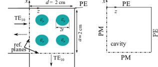
Fig. 12: A $90^{0}$ waveguide bend loaded with a cylindrical lossy dielectric post with constitutive parameters $\varepsilon_{r}=3,$ $\mu_{r}=1$, and $\tan\delta=0.01$ and the employed boundary conditions for the canonical modes used by the EPT are shown on the right.

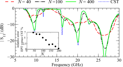
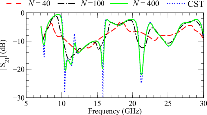
Fig. 13: (a) $|S_{11}|$ and (b) $|S_{21}|$ of the loaded waveguide bend shown in Fig. 12 computed using both EPT and full wave simulation (CST). The inset of (a) shows the relative error between EPT calcualted electric field in the cavity center compared to the one obtained using CST, for increasing $N$.

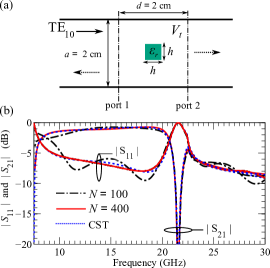
Fig. 14: (a) A dielectric obstacle (square post) inside a rectangular waveguide. (b) Scattering parameters of the loaded waveguide discontinuity shown in (a) computed using both EPT and CST.

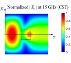
(a)

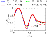
(b)

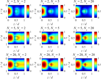
(c)

Fig. 15: (a) Electric field magnitude |$E_{y}$|, normalized ito its maximum inside the waveguide discontinuity in Fig. 14 (a) at 15 GHz obtained by CST. (b) Field along the z-direction for different N and showing a good convergence to that obtained by CST. (c) Field maps of the y-directed electric field at 15 GHz obtained using the EPT technique. Here the field is excited using the fundamental TE mode of the waveguide.

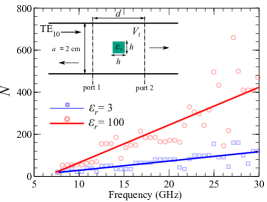
Fig. 16: The number of expansion modes required to achieve $\Delta S<1\%$ for $\varepsilon_{r}=$3 and 100 for the dielectric discontinuity in the inset. The symbols represent the calculations and the lines are the linear curve-fitting of $N$ with frequency based on (33).

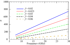
Fig. 17: Linear curve-fitting of the $N$ with frequency for different values of the volumetric filling factor $f$ for the case in the inset of Fig. 16.

V Conclusion

The eigenmode projection technique is demonstrated as a versatile technique for solving electromagnetic cavity resonance and guided-wave scattering problems. The solution procedure does not involve sub-wavelength segmentation of the structure under consideration as with other numerical techniques and can handle arbitrary-shaped structures with arbitrary loading in a straightforward manner. Convergence studies were conducted to estimate the number of modes required for the expansion to provide accurate results for both resonance and scattering problems relative to commercial solvers. Contrary to techniques like the Method of Moments, the EPT does not require dealing with structures with known Green’s functions as it is based on defining a canonical cavity enclosing the structure under study. Also, no singularity extraction process is needed (as in Green’s function based methods) nor divergence issues are encountered (as in finite-differences based methods) during the solution procedure. The EPT also gives the field distributions in the quasi-analytical form of a weighted sum of simple eigenmodes (sinusoids for rectangular cavities and Bessel functions for circular ones). A few examples were presented to verify the proposed technique in several scenarios. Other three-dimensional problems including radiation problems, printed circuits and others are yet to be investigated. For such problems, suitable choices of the canonical cavity, matrix filling, and port modeling are to be developed.

CAVITY EIGENMODES

The Helmholtz equations governing the solenoidal and irrotational eigenmodes can be solved upon enforcing the boundary conditions on the surface of the canonical cavity, which are

$$\text{For PM surface }\left\{\begin{array}[]{c}\mathbf{\hat{n}}\times\mathbf{H}_{n}=\mathbf{\hat{n}}\times\mathbf{G_{\lambda}}=\Psi_{\lambda}=\mathbf{0}\\ \mathbf{\hat{n}}\cdot\mathbf{E}_{n}=\mathbf{\hat{n}\cdot F_{\alpha}}=\partial\Phi_{\alpha}/\partial n=0\end{array}\right.$$ (34)

$$\text{For PE surface }\left\{\begin{array}[]{c}\mathbf{\hat{n}}\times\mathbf{E}_{n}=\mathbf{\hat{n}}\times\mathbf{F_{\alpha}}=\Phi_{\alpha}=\mathbf{0}\\ \mathbf{\hat{n}}\cdot\mathbf{H}_{n}=\mathbf{\hat{n}\cdot G_{\lambda}}=\partial\Psi_{\lambda}/\partial n=0\end{array}\right.$$ (35)

-A Circular Cylindrical Cavity

When solving problems illustrated in Figs. 3, 5 and 8, where the structure under investigation is a body of revolution around the $z$-axis, it is straight forward that the most appropriate choice of the canonical cavity in this problem is a finite-lenght circular cylinder with PEC walls. The cylinder radius $a$ and length $d$ are chosen such that it completely enclose the cavity. In this work, the solution is obtained for $\mathrm{TM^{z}}$ arbitrary cavity modes and the canonical cavity solenoidal and irrotational eigenmodes will be derived.

The cavity solenoidal modes are easily obtained by expanding the two curl equations in (3) with $\partial/\partial\phi=0$.

The group of solenoidal magnetic field modes inside the solenoidal cavity that will contribute to the ${\rm TM}{}_{z}$ mode excitation can be obtained by choosing $\mathbf{H}_{n}=\nabla\times\Pi_{z}\hat{\mathbf{a}}_{z}$ where $\Pi$ is the Hertz potential, and solving (5) subject to the boundary conditions (34) and (35), we get,

$$\mathbf{H}_{n}=H_{0n}J_{0}^{{}^{\prime}}(k_{n_{1}}\rho)\cos(k_{n_{2}}z)\hat{\mathbf{a}}_{\phi},$$ (36)

where $k_{n_{1}}=p_{0n_{1}}/a$, $k_{n_{2}}=n_{2}\pi/d$, and $k_{n}^{2}=k_{n_{1}}^{2}+k_{n_{2}}^{2}$; and $p_{0}{n_{1}}$ is the $n_{1}$th zero of $J_{0}\left(x\right)$. The constant $H_{0n}$ is determined such that the normalization condition $\int_{V_{t}}\mathbf{H}_{n}\cdot\mathbf{H}_{n}dv=1$ is satisfied.

The corresponding $\mathbf{E}_{n}$ modes family can be obtained from (3),

$$\mathbf{E}_{n}=\frac{k_{n_{2}}}{k_{n}}H_{n}J_{0}^{{}^{\prime}}\left(k_{n_{1}}\rho\right)\sin\left(k_{n_{2}}z\right)\hat{\mathbf{a}}_{\rho}\\ -\frac{k_{n_{1}}}{k_{n}}H_{n}J_{0}\left(k_{n_{1}}\rho\right)\cos\left(k_{n_{2}}z\right)\hat{\mathbf{a}}_{z}$$ (37)

Similarly, the irrotational modes,$\Phi_{\alpha}$ and the corresponding $\mathbf{F}_{\alpha}$, that couple to the azimothally symmetric $\textrm{TM}^{z}$ are obtained as,

$$\Phi_{\alpha}=U_{\alpha}J_{0}\left(l_{\rho}\rho\right)\sin\left(l_{z}z\right)$$

Hence, $\mathbf{F}_{\alpha}$ can be obtained from (5), and $l_{\alpha}^{2}=l_{z}^{2}+l_{\rho}^{2}$. The constant $U_{\alpha}$ is determined such that the normalization condition $\int_{V_{t}}\Phi_{\alpha}^{2}dv=\int_{V_{t}}\mathbf{F}_{\alpha}\cdot\mathbf{F}_{\alpha}dv=1$ is satisfied.

-B Rectangular Cavity

When solving for the structures in Figs. 12 and 16, the canonical cavity chosen would be a rectangular cavity resonator, where the waveguide ports will be treated as PM surfaces when calculating the cavity modes, while the rest of the walls is PE. As there is no variation in the structure geometry in the normal direction ($y$-direction), the excitation with $\textrm{TE}_{n0}^{z}$ would not couple to any other port modes. Moreover, the excited cavity modes would be of the type ${\rm TM_{n_{1}0n_{2}}^{y}}$.

The solenoidal electric field $\mathbf{E}_{n}$ modes for cavity in Fig. 12 will be given by,

$$\mathbf{E}_{n}=E_{n}\cos\left(k_{x}x\right)\cos\left(k_{z}z\right)\hat{\mathbf{a}}_{y},$$

and the corresponding magnetic field $\mathbf{H}_{n}$ can be obtained using Eq. (3), where $k_{x}=\left(2n_{1}-1\right)\pi/\left(2a\right)$, $k_{z}=\left(2n_{2}-1\right)\pi/\left(2d\right)$, and $k_{n}^{2}=k_{x}^{2}+k_{z}^{2}$.

The solenoidal electric field $\mathbf{E}_{n}$ modes for cavity in Fig. 16 will be given by,

$$\mathbf{E}_{n}=E_{n}\sin\left(k_{x}x\right)\cos\left(k_{z}z\right)\mathbf{a}_{y}$$

and the corresponding magnetic field $\mathbf{H}_{n}$ can be obtained using Eq. (3), where $k_{x}=n_{1}\pi/2a$, $k_{z}=n_{2}\pi/2d$, and $k_{n}^{2}=k_{x}^{2}+k_{z}^{2}$.

It is interesting to notice that irrotational modes will not couple to any of the port excitation $\textrm{TE}_{n0}^{z}$ nor to any of the previously mentioned ${\rm TM_{n_{1}0n_{2}}^{y}}$ solenoidal modes, for the special case of uniform posts along $y$-axis. Moreover, few port modes are considered to account for evanescent modes that are excited at the discontinuities.

References

- [1] A. Wexler, “Solution of waveguide discontinuities by modal analysis,” Microwave Theory and Techniques, IEEE Transactions on, vol. 15, pp. 508 –517, september 1967.
- [2] R. MacPhie and K.-L. Wu, “A full-wave modal analysis of arbitrarily shaped waveguide discontinuities using the finite plane-wave series expansion,” Microwave Theory and Techniques, IEEE Transactions on, vol. 47, pp. 232 –237, feb 1999.
- [3] D.-C. Liu, “On the theory of the modal expansion method for the em fields inside a closed volume,” Journal of Physics D: Applied Physics, vol. 36 no. 13, p. 1629, 2003.
- [4] R. MacPhie and K.-L. Wu, “A plane wave expansion of spherical wave functions for modal analysis of guided wave structures and scatterers,” Antennas and Propagation, IEEE Transactions on, vol. 51, pp. 2801 – 2805, oct. 2003.
- [5] K. Ogusu, “Numerical analysis of rectangular dielectric waveguide and its modifications,” Microwave Theory and Techniques, IEEE Transactions on, vol. vol. 25, no. 11, pp. 874–885, 1977.
- [6] C. Angulo, “Discontinuities in a rectangular waveguide partially filled with dielectric,” Microwave Theory and Techniques, IRE Transactions on, vol. 5, pp. 68 –74, january 1957.
- [7] F. Moglie, T. Rozzi, P. Marcozzi, and A. Schiavoni, “A new termination condition for the application of fdtd techniques to discontinuity problems in close homogeneous waveguide,” Microwave and Guided Wave Letters, IEEE, vol. 2, pp. 475 –477, dec. 1992.
- [8] Z. Lou and J.-M. Jin, “An accurate waveguide port boundary condition for the time-domain finite-element method,” Microwave Theory and Techniques, IEEE Transactions on, vol. 53, pp. 3014 – 3023, sept. 2005.
- [9] A. Belenguer, H. Esteban, V. Boria, C. Bachiller, and J. Morro, “Hybrid mode matching and method of moments method for the full-wave analysis of arbitrarily shaped structures fed through canonical waveguides using only electric currents,” Microwave Theory and Techniques, IEEE Transactions on, vol. 58, pp. 537 –544, march 2010.
- [10] P. Arcioni, M. Bressan, and L. Perregrini, “A new boundary integral approach to the determination of the resonant modes of arbitrarily shaped cavities,” Microwave Theory and Techniques, IEEE Transactions on, vol. 43, pp. 1848 – 1856, aug 1995.
- [11] P. Arcioni, M. Bozzi, M. Bressan, and L. Perregrini, “A novel cad tool for the wideband modeling of 3d waveguide components,” International Journal of RF and Microwave Computer-Aided Engineering, vol. 10, pp. 183 – 189, march 2000.
- [12] J. C. Slater, Microwave Electronics. Van Nostrand Company, 1950.
- [13] K. Kurokawa, “The expansions of electromagnetic fields in cavities,” Microwave Theory and Techniques, IRE Transactions on, vol. 6, pp. 178 –187, april 1958.
- [14] S. Schelkunoff, “Representation of impedance functions in terms of resonant frequencies,” Proceedings of the IRE, vol. 32, pp. 83 – 90, feb. 1944.
- [15] T. Teichmann and E. P. Wigner, “Electromagnetic field expansions in loss-free cavities excited through holes,” Journal of Applied Physics, vol. 24, pp. 262 –267, mar 1953.
- [16] S. A. Schelkunoff, “On representation of electromagnetic fields in cavities in terms of natural modes of oscillation,” Journal of Applied Physics, vol. 26, pp. 1231 –1234, oct 1955.
- [17] S. Cohn, “Design considerations for high-power microwave filters,” Microwave Theory and Techniques, IRE Transactions on, vol. 7, pp. 149 –153, january 1959.
- [18] J. Slater, “The design of linear accelerators,” Reviews of Modern Physics, vol. 20, no. 3, p. 473, 1948.
- [19] M. A. Othman, T. M. Abuelfadl, and I. A. Eshrah, “Analysis of microwave cavities using an eigenmode projection approach,” in Antennas and Propagation Society International Symposium (APSURSI), 2012 IEEE, pp. 1 –2, july 2012.
- [20] M. Nasr, I. Eshrah, and T. Abuelfadl, “Solution of electromagnetic scattering problems using an eigenmode projection technique,” in Antennas and Propagation Society International Symposium (APSURSI), 2013 IEEE, pp. 1312–1313, July 2013.
- [21] M. Nasr, I. Eshrah, and T. Abuelfadl, “Wideband analysis of scattering problems using an eigenmode projection technique,” in Microwave Conference (EuMC), 2013 European, pp. 1231–1234, Oct 2013.
- [22] M. A. Othman, I. A. Eshrah, and T. M. Abuelfadl, “Analysis of waveguide discontinuities using eigenmode expansion,” in IEEE International Microwave Symposium, 2013.
- [23] M. Nasr, I. Eshrah, and T. Abuelfadl, “Electromagnetic scattering from dielectric objects using the eigenmode projection technique,” Antennas and Propagation, IEEE Transactions on, vol. 62, pp. 3222–3231, June 2014.
- [24] H. Haskal, “Matrix description of waveguide discontinuities in the presence of evanescent modes,” Microwave Theory and Techniques, IEEE Transactions on, vol. 12, pp. 184 – 188, mar 1964.
- [25] T. K. Mealy, I. A. Eshrah, and T. M. Abuelfadl, “Solution of periodically loaded waveguides using the eigenmode projection technique,” in IEEE International Microwave Symposium, 2016.
- [26] I. A. Eshrah and T. M. Abuelfadl, “Electrostatic analysis of multiconductor transmission lines using an eigenmode projection technique,” in IEEE International Microwave Symposium, 2016.
- [27] J. G. V. Bladel, Electromagnetic Fields. IEEE Press Series on Electromagnetic Wave Theory, Wiely-Interscience, pp. 509-520, 2007.
- [28] R. E. Collin, Foundationws for Microwave Engineering. IEEE Press Series on Electromagnetic Wave Theory, Wiely-Interscience, pp. 525-540, 2001.
- [29] “CST©- Computer Simulation Technology.”
- [30] F. Gerigk, “Cavity types,” the CERN Accelerator School CAS 2010: RF for accelerators, 2011.
- [31] R. B. Marks and D. F. Williams, “A general waveguide circuit theory,” Journal of Research of the National Institute of Standards and Technology, vol. 97, p. no. 5, 1992.
- [32] R. Levy, “Determination of simple equivalent circuits of interacting discontinuities in waveguides or transmission lines,” Microwave Theory and Techniques, IEEE Transactions on, vol. 48, pp. 1712 –1716, oct 2000.
- [33] http://mathworld.wolfram.com/GibbsPhenomenon.html.