Depleted Depletion Drives Polymer Swelling in Poor Solvent Mixtures

Abstract

Macromolecular solubility in solvent mixtures often exhibit striking and paradoxical nature. For example, when two well miscible poor solvents for a given polymer are mixed together, the same polymer may swell within intermediate mixing ratios. We combine computer simulations and theoretical arguments to unveil the first microscopic, generic origin of this collapse-swelling-collapse scenario. We show that this phenomenon naturally emerges at constant pressure in mixtures of purely repulsive components, especially when a delicate balance of the entropically driven depletion interactions is achieved.

It has been commonly observed that a polymer can collapse in a mixture of two competing, well miscible good solvents, while the same polymer remains expanded in these two individual components. This phenomenon is commonly known as co-non-solvency [1, 2, 3, 4, 5, 6, 7, 8, 9, 10]. However, it has also been observed that a polymer can be collapsed in two different poor solvents, whereas it is “better” soluble in their mixtures [11, 12, 13, 14]. Thus far a multitude of specific, system dependent explanations hindered the emergence of a clear physical picture of these two intriguing phenomena. While the phenomenon of co-non-solvency has been recently brought onto a firmer ground of a generic explanation [8, 9], no equivalent understanding of the collapse-swelling-collapse behavior has yet been achieved. In this work we propose the microscopic, generic picture of this collapse-swelling-collapse behavior in poor solvent mixtures.

In a standard poor solvent, starting from a good solvent condition, an increase of the effective attraction between the monomers first brings the polymer into $\Theta-$conditions, where the radius of gyration scales as $R_{\rm g}\sim N_{l}^{1/2}$ with $N_{l}$ being the chain length [15, 16]. Upon further increase of the attraction, a polymer then collapses into a globular state. The resultant collapsed globule can be understood by balancing the negative second virial osmotic contributions and the three body repulsions. The effective attraction, between monomers of a polymer, originates when the solvent particles repel polymer beads more than the repulsion between two monomers [15, 16]. This attraction between monomer beads is referred to as depletion induced attraction, well known from colloidal stability [17]. In this case, the resulting isolated polymer conformation can be well described by the Porod scaling law of the static structure factor $S(q)\propto q^{-4}$, presenting a compact spherical globule. Interestingly, even if a polymer exhibits poor solvent conditions in two different solvents, it can possibly be somewhat swollen by intermediate mixing ratios of the two poor solvents. A system that shows this collapse-swelling-collapse scenario is poly(methyl methacrylate) (PMMA) in aqueous alcohol mixtures. More specifically, water and alcohol are almost perfectly miscible and individually poor solvents for PMMA. However, PMMA shows improved solubility within the intermediate mixing concentrations of aqueous alcohol and/or other solvent mixtures [11, 12, 13, 14].

In this work, we aim to (1) devise a thermodynamically consistent generic (chemically independent) model for a polymer in poor solvent mixtures, such that solubility of many polymers can be explained within a simplified (universal) physical concept, (2) develop a microscopic understanding of the collapse-swelling-collapse scenario, and (3) investigate if a polymer in mixed poor solvents can really reach a fully extended good solvent chain. To achieve the above goals, we combine generic molecular dynamics, all-atom simulations and theoretical arguments to study polymer solvation in poor solvent mixtures.

Our generic simulations are based on the well-known bead-spring model of polymers [18]. A bead-spring polymer $p$ is solvated in mixed solutions composed of two components, solvent $s$ and cosolvent $c$, respectively. The mole fraction of the cosolvent component $x_{c}$ is varied from 0 (pure $s$ component) to 1 (pure $c$ component). Simulations are performed using the ESPResSo++ molecular dynamics package [19]. We have also performed all-atom simulations using the GROMACS molecular dynamics package [20]. The details about generic simulations and all-atom force field parameters are given in the electronic supplementary material [21].

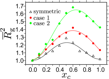
Figure 1: Normalized squared radius of gyration ${\overline{R}}_{\rm g}^{2}=\left<R_{\rm g}^{2}\right>/\left<R_{\rm g}(x_{c}=0)^{2}\right>$ as a function of cosolvent molar concentration $x_{c}$. Results are shown for the generic simulations and for three different cases. The parameters specific details of generic cases are listed in the electronic supplementary material [21]. The results are shown for a chain length of $N_{l}=30$. Lines are polynomial fits to the data that are drawn to guide the eye.

In Fig. 1 we summarize results for the normalized squared radius of gyration ${\overline{R}}_{\rm g}^{2}=\left<R_{\rm g}^{2}\right>/\left<R_{\rm g}(x_{c}=0)^{2}\right>$ as a function of $x_{c}$ from the generic model and for three different cases described in the supplementary material [21]. A closer look at the symmetric case of two almost perfectly miscible solvents (black $\triangle$) show that $-$ while the pure solvent ($x_{c}=0$) and the pure cosolvent ($x_{c}=1$) are equally poor solvents for the polymer, the same polymer swells within the intermediate cosolvent compositions reaching maximum swelling of ${\overline{R}}_{\rm g}^{2}$ by $\sim 20\%$ at around $x_{c}=0.5$. How could this be? In this context, given that this is a case of standard poor solvent collapse, the polymer conformations are given by depletion forces (or depletion induced attraction) [17]. Using simple depletion arguments, when both solvent and cosolvent are equally repulsive, polymer conformation should remain unaltered over the full range of $x_{c}$. Here, however, when cosolvents are added into polymer-solvent system (such as the addition of alcohol in PMMA-water system), the addition of cosolvents not only deplete monomers, but also deplete solvents. This leads to an effective double depletion effect that ultimately gives rise to a reduced depletion around $x_{c}=0.5$ and thus is consistent with the swelling of the polymers. Note that the depletion forces are intimately linked to the total density of system $\rho_{\rm total}$ and, therefore, reduced depletion forces should also be associated with the reduced $\rho_{\rm total}$. Interestingly, when looking into aqueous-alcohol mixtures, it becomes clear that $\rho_{\rm total}$ of the solution at constant pressure $P$ does not change linearly with changing composition (or $x_{c}$) [22]. Instead, they exhibit a minimum in $\rho_{\rm total}$ around $x_{c}=0.5$ (see Fig. 1 in electronic supplementary material [21]), indicating that the miscibility is only almost perfect. In our generic simulations, we have tuned solvent-cosolvent (repulsive) interaction strength $\epsilon_{sc}$ such that the generic system can reproduce the weak density dip observed in the aqueous alcohol mixtures at constant $P$, see Fig. 2(a). Furthermore, the system parameters are chosen such that the bulk solution remains deep into the miscible state far from the phase separation. The representative simulation snapshot is shown in Fig. 2(b) for a $50-50$ solvent-cosolvent mixture.

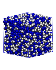
Figure 2: Simulation snapshots of the generic system presenting bulk solution for a $x_{c}=0.5$ mixture.

When the interaction asymmetry between polymer-cosolvent $\epsilon_{pc}$ and polymer-solvent $\epsilon_{ps}$ is increased (see electronic supplementary material [21]), where $\epsilon_{pc}$ for case 2 $<$ case 1 $<$ symmetric case, not only that the degree of swelling increases, but the swelling region also shifts between $0.5<x_{c}<0.9$. This range is found to be in excellent agreement with the experimental observation of PMMA conformation in aqueous alcohol mixtures [12, 13]. Furthermore, our case 2 is closely resembles PMMA in aqueous methanol mixture, where we tune parameters to mimic PMMA in aqueous methanol mixtures (see electronic supplementary material [21]). A closer look at Fig. 1 shows that the degree of swelling, within the range $0.5<x_{c}<0.9$, varies between 20-65% (or 10-30% in $\overline{R}_{\rm g}$) depending on the interaction assymetry. Considering that we are dealing with combinations of poor solvents, this is a very significant swelling. Moreover, analyzing the simulation it becomes apparent that the polymer does not neccesarily reach a fully expanded configuration. A quantity that perhaps best quantifies a polymer conformation is the static structure factor $S(q)$. In Fig. 3 we present $S(q)$ for two different values of $x_{c}$ for the system described by case 1. Part (a) shows $S(q)$ of a fully collapsed chain in pure solvent ($x_{c}=0$) and part (b) presents maximum polymer swelling ($x_{c}=0.7$).

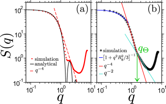
Figure 3: Static structure factor $S(q)$ for a chain of length $N_{l}=100$. Part (a) shows $S(q)$ at $x_{c}=0.0$ and part (b) for $x_{c}=0.7$. In part (a) we also include the analytical expression for the sphere scattering. In part (b) red and green lines are power law fits to the data at different length scales. Blue line represents Gruiner region for $q\to 0$ (for large length scales). Vertical arrow indicates the effective $\Theta-$blob size at $q=q_{\Theta}$, estimated using $\ell_{\Theta-{\rm blob}}=2\pi/q_{\Theta}$. Note to get better estimation of the cross-over scaling regime, $S(q)$ is calculated from a simulation of a chain length $N_{l}=100$.

For $x_{c}=0.0$, the polymer can be well described by a scaling law known for sphere scattering (Porod scattering), namely $S(q)\sim q^{-4}$, suggesting a fully collapsed poor solvent conformation. Furthermore, the data point corresponding to $x_{c}=0.7$ shows more interesting polymer conformations. Within the range $1.5{\sigma^{-1}}<q<3.0{\sigma^{-1}}$ an aparent scaling $S(q)\sim q^{-2}$ is observed, which crosses over to $S(q)\sim q^{-4}$ for $0.7{\sigma^{-1}}<q<1.5{\sigma^{-1}}$, suggesting that the polymer remains globally collapsed consisting of $\Theta-$blobs. The crossover point $q_{\Theta}$ gives the direct measure of the effective blob size $\ell_{\Theta-{\rm blob}}=2\pi/q_{\Theta}$. The largest blobs are observed when the polymer is maximally swollen.

Phase transition in polymer solutions, including the determination of changes in solvent quality leading to polymer collapse, are conveniently described at the mean-field level by the Flory-Huggins (FH) theory and its variants. For the case where a polymer with chain length $N_{l}$, at volume fraction $\phi_{p}$, is dissolved in a mixture of two components $s$ and $c$, respectively, FH theory predicts a monomer-monomer excluded volume of the form [15, 16],

$$\overline{\mathcal{V}} = 1-2\left(1-x_{c}\right)\chi_{ps}-2x_{c}\chi_{pc}+2x_{c}\left(1-x_{c}\right)\chi_{sc},$$ (1)

where $\chi_{ps}$ and $\chi_{pc}$ are the Flory-Huggins interaction parameters between $p-s$ and $p-c$, respectively. The factor $\chi_{sc}$ is the parameter of $s-c$ interaction. When both solvent and cosolvent are poor solvents, $\chi_{ps}>1/2$ and $\chi_{pc}>1/2$. In our simulations $\overline{\mathcal{V}}={\mathcal{V}}/\mathcal{V}_{\rm m}$ is calculated using the expression ${\mathcal{V}}=2\pi\int\left[1-e^{-v(r)/k_{\rm B}T}\right]r^{2}dr$. We use $v(r)=-k_{\rm B}T\ln\left[{\rm g}(r)\right]$ as a guess of the potential of mean force (PMF), which is calculated from the radial distribution function between non-bonded monomers ${\rm g}(r)$. $\mathcal{V}_{\rm m}=2.73~{}\sigma^{3}$ is the bare monomer excluded volume in the absence of any (co)solvent and corresponds to a monomer-monomer distance of $0.87\sigma$. Fitting Eq. 1 to the $\overline{\mathcal{V}}$ data in Fig. 4, we find $\chi_{ps}=1.57$, $\chi_{pc}=1.11$ and $\chi_{sc}=1.74$ for case 1 and $\chi_{ps}=1.62$, $\chi_{pc}=0.95$ and $\chi_{sc}=1.74$ for case 2. Consistently $\chi_{sc}$ values for both cases are similar, since this parameter is independent of polymer solvent interactions. Note also that standard FH predictions assume that solvent and cosolvent $-$ and also polymer $-$ are mixed at constant volume, whereas our simulations and experiments are performed at a constant pressure. In the following we derive a FH expression for the $\mathcal{V}$ values at constant $p$, which predicts reduced effective values for $\chi_{sc}$ dependent on $p$.

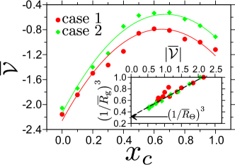
Figure 4: Normalized excluded volume $\overline{\mathcal{V}}={\mathcal{V}}/\mathcal{V}_{\rm m}$ as a function of cosolvent mole fraction $x_{c}$. Results are shown for two cases. Lines are fits to the data corresponding to Eq. 1. In the inset we present $\left(1/{\overline{R}}_{\rm g}\right)^{3}$ as a function of normalized $\mathcal{V}$. Here, ${\overline{R}}_{\rm g}=R_{\rm g}/R_{\rm g}(x_{c}=0)$ is the normalized gyration radius $R_{\rm g}$. The line is a fit based on Eq. 5.

In our simulations, we only consider polymer under infinite dilution $\phi_{p}\to 0$ and the large majority of the volume is occupied by solvent-cosolvent mixture. Therefore, we concentrate our analysis on the binary mixture. Additionally, we also consider that the pure reference solvent and cosolvent systems are identical, but that $s-c$ interactions are distinct from those for $s-s$ and $c-c$. For this case, the total free energy is written as

$$\frac{{\mathcal{F}}{v}}{\kappa_{\rm B}T} = \frac{{v}{\mathcal{F}}_{s}({v})}{\kappa_{\rm B}T}+x_{c}\ln(x_{c})+(1-x_{c})\ln(1-x_{c})$$ (2)

$$+ \chi_{sc}({v})x_{c}(1-x_{c}),$$

where ${\mathcal{F}}_{s}({v})$ is the volume-dependent free-energy of the pure solvent or cosolvent systems and where we consider the explicit dependence of $\chi_{sc}$ on system volume. Note that since experiments and simulations are performed at constant number of molecules ${\mathcal{N}}$, the total volume of the system $V$ is simply given by $V={\mathcal{N}}{v}$. For a given external pressure $P$, the molar volume ${v}$ is thus controlled by, $P=P_{s}({v})-{\kappa_{\rm B}T}x_{c}(1-x_{c}){\partial\chi_{sc}({v})}/{\partial{v}}$ with $P_{s}({v})=-\partial{v}{\mathcal{F}}_{s}/\partial{v}$ being the pressure of the reference system. If one assumes a small variation of the molar volume of the solvent-cosolvent mixture with respect to that of the reference system, one gets

$${v}={v_{\rm o}}\left[1+\zeta\ x_{c}(1-x_{c})\right],$$ (3)

where $\zeta={\kappa_{\rm B}T}/{v}\ \partial\chi_{sc}({v})/\partial{v}\left[\partial P_{s}({v})/\partial{v}\right]^{-1}$ measures the relative sensitivity of the interaction parameter and reference pressure to ${v}$. In supplementary material [21] we show $P_{s}$ as a function of $v$ that gives an estimate of $\partial P_{s}({v})/\partial{v}=20\epsilon/\sigma^{6}$. Eq. 3 describes well the observed density variation of the generic model in Fig. 2(a) with $\zeta=0.26$. Note that $\rho_{\rm total}$ and molar volume $v$ are simply related by $\rho_{\rm total}=1/{v}$. Also to first order in $({v}-{v_{\rm o}})/{v_{\rm o}}$, which for our generic model is of the order of 10%, one gets

$$\chi_{sc}({v}) = \chi_{sc}({v_{\rm o}})+{v}\frac{\partial\chi_{sc}({v})}{\partial{v}}{\bigg{|}_{x_{c}\to 0}}\zeta x_{c}(1-x_{c}),$$ (4)

thus showing that the interaction parameter is only perturbed to second order in beta. This will lead to an effective expression $\chi_{sc}({v})=\chi_{sc}({v_{\rm o}})-0.089x_{c}(1-x_{c})$. Incorporating Eq. 4 into Eq. 1 gives rise to the collapse-swelling-collapse scenario shown in Fig. 4. Furthermore, if we choose $x_{c}=0.5$, the above equation will lead to a $\sim 2\%$ variation in $\chi_{sc}$ values with respect to the standard values calculated in NVT ensemble. This suggests that $-$ while the phenomenon naturally emerges at constant $P$, the constant volume (lattice models), though not appropriate, could still reasonably work because of a small deviation of $\chi_{sc}$ between two ensembles. However, one should also note that on a lattice it is difficult to speak of constant $P$.

Our numerical predictions successfully account for polymer swelling in solutions of poor solvent mixtures. The simulations quantitatively confirm that $-$ while this fascinating polymer behavior is driven by purely repulsive interactions, they also reveal the subtle balance of local depletion forces and the bulk solution properties behind the paradoxical nature of such phenomena. Indeed, polymer collapse in repulsive solvents can be understood by depletion induced attractions [17]. The dominant contribution to the depletion attraction potentials originates from the direct monomer-solvent repulsions, and is thus proportional to solvent number density $\rho_{\rm totat}$ dictating number of depletants. When a few solvent molecules are replaced by cosolvents, for example a water by an alcohol, preserves, at first order in solvent density, a linear composition rule for the total strength of the attractions, especially for simulations under NVT ensemble. Under these conditions one should smoothly interpolate between two polymer collapsed states, without any swelling at intermediate compositions. Here, however, interactions between solvent components play a delicate role in dictating the depletion forces, bringing in contributions proportional to the square (or to even higher powers) of $\rho_{\rm total}$, see Fig. 2(a). The dominant effect of these solvent-cosolvent (depletant-depletant) interactions is to reduce the total depletion attractions. Such effects can be understood by noticing that any (co)solvent molecule present between two monomers already depletes a significant number of particles from its vicinity and thus reduces the number of depletants contributing to the total monomer-monomer attraction. In our case reduction of polymer collapse is obtained, enhanced and tuned by a solvent-cosolvent excluded volume that is slightly stronger than the corresponding values for solvent-solvent and cosolvent-cosolvent molecules. At intermediate compositions, where solvent-cosolvent interactions are dominant, there is a stronger reduction of the attractive depletion forces leading to polymer collapse, thus allowing for a significant polymer swelling. In practice, therefore, a broad variety of polymer/solvent systems are expected to display such behavior provided that both repulsive solvents have mutual interactions, leading to depletion of depletion forces.

A standard measure of the attractive forces leading to polymer collapse is provided by the monomer excluded volume $\mathcal{V}$. For poor solvents $\mathcal{V}$ is negative, and the dimensions of the chain can be understood by balancing the second (negative) virial osmotic contributions and the three body repulsion [15, 16], leading to

$$\frac{{\overline{R}_{\Theta}}^{3}}{{\overline{R}_{\rm g}}^{3}}-{1}=|\overline{\mathcal{V}}|.$$ (5)

In the inset of Fig. 4 we show $\left(1/{\overline{R}}_{\rm g}\right)^{3}$ as a function of $\overline{\mathcal{V}}$, where the $R_{\rm g}$ is taken from Fig. 1(a) and $\overline{\mathcal{V}}$ is given by the values in the main panel of Fig. 4. The data is well described by the theoretical prediction in Eq. 5. Extrapolating the data to $\mathcal{V}=0$, we estimate ${\overline{R}}_{\Theta}=1.46$ (or $R_{\Theta}=2.34\sigma$), further suggesting that the polymer remains below $\Theta-$conformation, even when it swells within intermediate mixing ratios.

This collapse-swelling-collapse scenario of PMMA in aqueous alcohol appears as the opposite effect to that of coil-globule-coil scenario of PNIPAm in aqueous alcohol, often referred to as co-non-solvency [2, 3, 8]. However, the coil-globule-coil transitions are dictated by effects of solvent and cosolvent preferential adsorption [8], while the collapse-swelling-collapse behavior, studied here, is due to a subtle balance of depletion forces. Furthermore, our analysis also suggests that, contrary to the co-non-solvency effect that cannot be described by a Flory-Huggins mean-field picture, the mean-field behavior drives the collapse-swelling-collapse sequence in poor solvent mixtures. Here, the solvent-cosolvent interaction parameter $\chi_{sc}$, though quite small, plays a key role. Our results clarify that although collapse-swelling-collapse and co-non-solvency appear as two symmetric manifestations of polymer solubility, they are in fact driven by markedly different physical mechanisms.

In conclusion, we have performed molecular dynamics simulations to unveil the microscopic origin of polymer swelling in poor solvent mixtures. We propose a unified generic picture of the polymer collapse-swelling-collapse transition. This conformational transition is due to a delicate balance between the depletion forces and the bulk solution density at constant pressure. Combining Flory-Huggins type mean field picture with molecular dynamics simulations, we show that the polymer swelling in poor solvents is dictated by reduced depletion forces that ordinate because the bulk solution properties. More interestingly, these results show striking quantitative agreement with the experimental data obtained from PMMA solvated in aqueous alcohol and all-atom simulations. While the polymer swell significantly, the mostly swollen polymer structure still remains below $\Theta-$conformation.

Acknowledgment: D.M. thanks Burkhard Dünweg and Vagelis Harmandaris for many stimulating discussions, Tiago Oliveira for the help to build the all-atom PMMA force field and Björn Baumeier for suggesting Ref. [4] in supplementary material [21]. C.M.M. acknowledges Max-Planck Institut für Polymerforschung for hospitality where this work was initiated and performed. We thank Nancy Carolina Forero-Martinez and Hsiao-Ping Hsu for critical reading of the manuscript.

References

- [1] B. A. Wolf and M. M. Willms, Makromol. Chem. 179, 2265 (1978).
- [2] H. G. Schild, M. Muthukumar, and D. A. Tirrell, Macromolecules 24, 948 (1991).
- [3] G. Zhang and C. Wu, Phys. Rev. Lett. 86, 822 (2001).
- [4] A. Hiroki, Y. Maekawa, M. Yoshida, K. Kubota, and R. Katakai, Polymer 42, 1863 (2001).
- [5] Y. Kiritoshi and K. Ishihara, Sci. Technol. Adv. Mater. 4, 93 (2003).
- [6] R. Lund, L. Willner, J. Stellbrink, A. Radulescu, and D. Richter, Macromolecules 37, 9984 (2004).
- [7] D. Mukherji and K. Kremer, Macromolecules 46, 9158 (2013).
- [8] D. Mukherji, C. M. Marques, and K. Kremer, Nat. Commun. 5 4882 (2014).
- [9] D. Mukherji, C. M. Marques, T. Stuehn, and K. Kremer, J. Chem. Phys. 142, 114903 (2015).
- [10] J. Dudowicz, K. F. Freed, and J. F. Douglas, J. Chem. Phys. 143, 131101 (2015).
- [11] R. M. Masegosa, M. G. Prolongo, I. Hernandez-Feures, and A. Horta, Macromolecules, 17, 1181 (1984).
- [12] R. Hoogenboom, C. Remzi Becer, C. Guerrero-Sanchez, S. Hoeppener, and U. S. Schubert, Aust. J. Chem. 63 1173 (2010).
- [13] S. M. Lee and Y. C. Bae, Polymer 55 4684 (2014).
- [14] Y. Yu, B. D. Kieviet, E. Kutnyanszky, G. J. Vancso, and S. de Beer, ACS Macro Letters 4 75 (2015).
- [15] P.-G. de Gennes, Scaling Concepts in Polymer Physics (Cornell University Press, London, 1979).
- [16] J. Des Cloizeaux and G. Jannink, Polymers in Solution: Their Modelling and Structure (Clarendon Press, Oxford, 1990).
- [17] H. N. W. Lekkerkerker and R. Tuinier, Colloids and the Depletion Interaction (Clarendon Press, Oxford, 1990).
- [18] K. Kremer and G. S. Grest, J. Chem. Phys. 92, 5057 (1990).
- [19] J. D. Halverson, T. Brandes, O. Lenz, A. Arnold, S. Bevc, V. Starchenko, K. Kremer, T. Stuehn, D. Reith, Comp. Phys. Comm. 184, 1129 (2013)
- [20] S. Pronk, S. Pall, R. Schulz, P. Larsson, P. Bjelkmar, R. Apostolov, M. R. Shirts, J. C. Smith, P. M. Kasson, D. van der Spoel, B. Hess, and E. Lindahl, Bioinformatics 29, 845 (2013).
- [21] Electronic auxilliary material. Number to be filled by the editor.
- [22] A. Perera, F. Sokolic, L. Almasy, and Y. Koga, J. Chem. Phys. 124, 124515 (2006).