Efficient simulation for dependent rare events

Abstract

We consider the general problem of estimating probabilities which arise as a union of dependent events. We propose a flexible series of estimators for such probabilities, and describe variance reduction schemes applied to the proposed estimators. We derive efficiency results of the estimators in rare-event settings, in particular those associated with extremes. Finally, we examine the performance of our estimators in a numerical example.

1 Introduction

The estimators in this paper apply to quite general problems, so we will first introduce them in the framework of our main example, namely, as estimators relating to rare maxima of dependent random vectors. For a random vector $\bm{X}=(X_{1},\dots,X_{d})$ with maximum $M=\max_{i}X_{i}$, the first problem we consider is estimating

$$\alpha(\gamma)=\operatorname{{\mathbb{P}}}(M>\gamma)\,.$$

This problem has many applications in many areas, for example in actuarial science (e.g. default probabilities RP2 ), finance (e.g. probability of ‘knock-out’ in a barrier option cont2010encyclopedia ), survival analysis, reliability rausand2004system and engineering (e.g. failure probability of a series circuit).

We construct estimators for this probability, which are in terms of

$$E(\gamma)=\sum_{i=1}^{d}\mathds{1}\{X_{i}>\gamma\}\,,$$

the random variable which counts the number of $X_{i}$ which exceed $\gamma$. Our two main estimators in this setting are

$$\widehat{\alpha}_{1} =\sum_{i=1}^{d}\operatorname{{\mathbb{P}}}(X_{i}>\gamma)+\frac{1}{R}\sum_{r=1}^{R}(1-E_{r}(\gamma))\mathds{1}\{E_{r}(\gamma)\geq 2\}\,,\text{ and}$$ (1)

$$\widehat{\alpha}_{2} =\sum_{i=1}^{d}\operatorname{{\mathbb{P}}}(X_{i}>\gamma)-\sum_{i=1}^{d-1}\sum_{j=i+1}^{d}\operatorname{{\mathbb{P}}}(X_{i}>\gamma,X_{j}>\gamma)$$ (2)

$$\quad+\frac{1}{R}\sum_{r=1}^{R}\Big{[}1-E_{r}(\gamma)+\frac{E_{r}(\gamma)(E_{r}(\gamma)-1)}{2}\Big{]}\mathds{1}\{E_{r}(\gamma)\geq 3\}\,.$$

where $R\in{\mathbb{N}}$ and the $E_{r}(\gamma)$s are derived from i.i.d. samples of $\bm{X}$. The fact that these are unbiased estimators of $\alpha(\gamma)$ follows from Proposition 1 below. Estimation of $\operatorname{{\mathbb{P}}}(M>\gamma)$ is a difficult problem and treatments in the literature make distributional assumptions on $\bm{X}$. One such example is Adler et al. adler2012efficient where $\bm{X}$ is assumed to be multivariate normal. In this case, our estimator $\widehat{\alpha}_{1}$, with appropriate importance sampling, is the same as one of the estimators from adler2012efficient .

The next problem we consider is estimating

$$\beta_{n}(\gamma):=\operatorname{\mathbb{E}}[Y\mathds{1}\{E(\gamma)\geq n\}]$$

for $n=1,\dots,d$ and some random variable $Y$. We do not make any assumptions of independence between the $\{X_{i}>\gamma\}$ events themselves or between the events and $Y$.

The subcase of $Y=1$ a.s. has some interesting examples:

$$\beta_{1}(\gamma)=\operatorname{{\mathbb{P}}}(M>\gamma)=\alpha(\gamma)\,,\quad\text{and}\quad\beta_{n}(\gamma)=\operatorname{{\mathbb{P}}}(X_{(n)}>\gamma)$$

where $X_{(1)}\geq X_{(2)}\geq\dots\geq X_{(d)}$ are the order statistics of $\bm{X}$. The probability of a parallel circuit failing is a simple application for $\operatorname{{\mathbb{P}}}(X_{(n)}>\gamma)$.

Our main $\beta_{1}$ estimator uses the fact that

$$\{M>\gamma\}:=\bigcup_{i=1}^{d}\{X_{i}>\gamma\}=\bigcup_{i=1}^{d}\{X_{1}\leq\gamma,\dots,X_{i-1}\leq\gamma,X_{i}>\gamma\}$$ (3)

where the events in the union on the right are disjoint. This supplies a form of $\beta_{1}$ which is amenable to efficient Monte Carlo estimation:

$$\beta_{1}=\sum_{i=1}^{d}\operatorname{\mathbb{E}}[Y\,\mathds{1}\{X_{1}\leq\gamma,\dots,X_{i-1}\leq\gamma\}\mid X_{i}>\gamma]\operatorname{{\mathbb{P}}}\left(X_{i}>\gamma\right)\,.$$ (4)

As previously mentioned, while they are main example and motivation, the extremes considered so far are a very specific instance of estimators. We now turn our attention to the general set-up treated in the paper.

Let $A(\gamma)=\cup_{i=1}^{d}A_{i}(\gamma)$ be the union of events $A_{1}(\gamma),\dots,A_{d}(\gamma)$ for an index parameter $\gamma\in\mathbb{R}$. We consider the problem of estimating $\operatorname{{\mathbb{P}}}(A(\gamma))$ when the events are rare, that is, $\operatorname{{\mathbb{P}}}(A(\gamma))\to 0$ as $\gamma\to\infty$. Define

$$\alpha(\gamma):=\operatorname{{\mathbb{P}}}(A(\gamma))\quad\text{and}\quad\quad E(\gamma):=\sum_{i=1}^{d}\mathds{1}\{A_{i}(\gamma)\}\,.$$

Note that we recover our introductory example by having $A_{i}(\gamma)=\{X_{i}>\gamma\}$. Aside from this example, $A(\gamma)$ is quite general (a union of arbitrary events) and many interesting events arising in applied probability and statistics can be formulated as a union. The quantity $\beta_{n}(\gamma)$ is reminiscent of expected shortfall from risk management mcneil2015quantitative .

Traditional Monte Carlo methods are unreliable in the rare-event setting. We will use standard techniques from the rare-event simulation methodology, such as importance sampling for variance reduction and applicable measures of efficiency: bounded relative error and logarithmic efficiency, cf. asmussen2007stochastic ; glasserman2003monte ; rubinstein2011simulation . The resulting estimators are among the most efficient possible under the most general assumptions.

The paper is structured as follows. In Sections 2 and 3 we formally introduce our estimators for $\alpha(\gamma)$ and $\beta_{n}(\gamma)$ respectively, we prove their validity, and show how to combine them with some existing variance reduction techniques; the efficiency properties for the general estimators are analysed in Section 4, in addition we further investigate the efficiency for certain important dependence structures. Finally, we evaluate the numerical performance of the estimators in Section 5.

2 Estimators of $\alpha$

In the following, we first explain the construction of our estimators of $\alpha$, then discuss possible variance reduction schemes. As the $\gamma$ notation can be cumbersome, we simply write $A=A(\gamma)$, $A_{i}=A_{i}(\gamma)$, $E=E(\gamma)$, $\alpha=\alpha(\gamma)$ and $\beta_{n}=\beta_{n}(\gamma)$. Similarly, we often write $\sum_{i}$, $\sum_{i<j}$, $\cup_{i}$, $\cap_{i}$ for $\sum_{i=1}^{d}$,$\sum_{1=i<j}^{d}$, $\cup_{i=1}^{d}$ and $\cap_{i=1}^{d}$.

2.1 Proposed estimators of $\alpha$

The inclusion–exclusion formula (IEF) provides a representation of $\alpha$ as a summation whose terms are decreasing in size. The formula is

$$\alpha=\operatorname{{\mathbb{P}}}(A)=\sum_{i=1}^{d}(-1)^{i+1}\sum_{|I|=i}\operatorname{{\mathbb{P}}}\Big{(}\bigcap_{i\in I}A_{i}\Big{)}\,.$$ (5)

The IEF can rarely be used as its summands are increasingly difficult to calculate numerically. The $\operatorname{{\mathbb{P}}}(A_{i})$ terms are typically known, and the $\operatorname{{\mathbb{P}}}(A_{i},A_{j})$ terms can frequently be calculated, however the remaining higher-dimensional terms are normally intractable for numerical integration algorithms (cf. the curse of dimensionality (asmussen2007stochastic, , Chapter IX)). Truncating the summation leads to bias, and indeed by the Bonferroni inequalities we have:

$$\alpha \leq\sum_{i=1}^{k}(-1)^{i-1}\sum_{|I|=i}\operatorname{{\mathbb{P}}}\Big{(}\bigcap_{i\in I}A_{i}\Big{)}\quad\text{ if }1\leq k<d\text{ and }k\text{ is odd},$$ (6)

$$\alpha \geq\sum_{i=1}^{k}(-1)^{i-1}\sum_{|I|=i}\operatorname{{\mathbb{P}}}\Big{(}\bigcap_{i\in I}A_{i}\Big{)}\quad\text{ if }1<k<d\text{ and }k\text{ is even}.$$ (7)

This higher-order intractability motivates our estimators which use the IEF rewritten in terms of $E=\sum_{i}\mathds{1}\{A_{i}\}$.

Proposition 1

For $i=1,\dots,d$,

$$\sum_{|I|=i}\mathds{1}\left\{\cap_{i\in I}A_{i}\right\}=\Bigl{(}{{E}\atop i}\Bigr{)}\mathds{1}\{E\geq i\}\,.$$ (8)

Proof

$$\sum_{|I|=i}\mathds{1}\{\cap_{i\in I}A_{i}\}=\sum_{k=i}^{d}\sum_{|I|=i}\mathds{1}\{\cap_{i\in I}A_{i},E=k\}=\sum_{k=i}^{d}\Bigl{(}{{k}\atop i}\Bigr{)}\mathds{1}\{E=k\}=\Bigl{(}{{E}\atop i}\Bigr{)}\mathds{1}\{E\geq i\}\,.$$

∎

Taking the expectation of (8) gives

$$\sum_{|I|=i}\operatorname{{\mathbb{P}}}\Big{(}\bigcap_{i\in I}A_{i}\Big{)}=\operatorname{\mathbb{E}}\Big{[}\Bigl{(}{{E}\atop i}\Bigr{)}\mathds{1}\{E\geq i\}\Big{]}\quad\text{ for }i=1,\dots,d\,.$$

So the following has mean $\alpha$, and forms the nucleus of our $\widehat{\alpha}_{i}$ estimators:

$$\sum_{i=1}^{d}(-1)^{i-1}\Bigl{(}{{E}\atop i}\Bigr{)}\mathds{1}\{E\geq i\}\,.$$ (9)

We present estimators which deterministically calculate the first larger terms of the IEF (5) and Monte Carlo (MC) estimate the remaining smaller terms using sample means of (8). We begin by constructing the single-replicate estimator $\widehat{\alpha}_{1}$ where the first summand is calculated and the remaining terms are estimated:

$$\widehat{\alpha}_{1}: =\sum_{i}\operatorname{{\mathbb{P}}}(A_{i})+\sum_{i=2}^{d}\Big{[}(-1)^{i-1}\Bigl{(}{{E}\atop i}\Bigr{)}\mathds{1}\{E\geq i\}\Big{]}$$

$$=\sum_{i}\operatorname{{\mathbb{P}}}(A_{i})+(1-E)\mathds{1}\{E\geq 2\}\,,\quad\text{using}\quad\sum_{k=0}^{n}(-1)^{k-1}\Bigl{(}{{n}\atop k}\Bigr{)}=0\,.$$

In identical fashion, the single-replicate estimator calculating the first two terms from the IEF is

$$\widehat{\alpha}_{2}:= \sum_{i}\operatorname{{\mathbb{P}}}(A_{i})-\sum_{i<j}\operatorname{{\mathbb{P}}}(A_{i},A_{j})+\sum_{i=3}^{d}\Big{[}(-1)^{i-1}\Bigl{(}{{E}\atop i}\Bigr{)}\mathds{1}\{E\geq i\}\Big{]}$$

$$= \sum_{i}\operatorname{{\mathbb{P}}}(A_{i})-\sum_{i<j}\operatorname{{\mathbb{P}}}(A_{i},A_{j})+\Big{[}1-E+\frac{E(E-1)}{2}\Big{]}\mathds{1}\{E\geq 3\}\,.$$

Thus, for $n\in\{1,\dots,d-1\}$,

$$\widehat{\alpha}_{n}:=\sum_{i=1}^{n}(-1)^{i-1}\sum_{|I|=i}\operatorname{{\mathbb{P}}}\Big{(}\bigcap_{i\in I}A_{i}\Big{)}+\Big{[}\sum_{i=0}^{n}(-1)^{i}\Bigl{(}{{E}\atop i}\Bigr{)}\Big{]}\mathds{1}\{E\geq n+1\}\,.$$ (10)

Thus, $\{\widehat{\alpha}_{1},\dots,\widehat{\alpha}_{d-1}\}$ is a collection of estimators which allows the user to control the computational division of labour between numerical integration and Monte Carlo estimation. We will furthermore let $\widehat{\alpha}_{0}$ be the crude Monte Carlo estimator $\mathds{1}\{E\geq 1\}$, and note that this falls under the definition in $\eqref{hat_alpha_n}$ if we interpret the empty sum as zero.

The $\widehat{\alpha}_{n}$ estimators are of decreasing variance in $n$, however each estimator carries the assumption that one can perform accurate numerical integration for $1$ up to $n$ dimensions. As numerical integration can be slow and unreliable in high dimensions we focus on $\widehat{\alpha}_{1}$, and also show the numerical performance of $\widehat{\alpha}_{2}$.

In practice, theses estimators will exhibit very modest improvements when compared against their truncated IEF counterparts (i.e., the right side of (6) and (7)). When combined with importance sampling, as in Section 2.4, the improvement is marked. Furthermore, we will show that these estimators possess desirable efficiency properties which are preserved after combining with importance sampling.

2.2 Discussion of $\widehat{\alpha}_{1}$ estimator

The estimator $\widehat{\alpha}_{1}$ has some nice interpretations. Recall the Boole–Fréchet inequalities

$$\max_{i}\,\operatorname{{\mathbb{P}}}(A_{i})\leq\alpha=\operatorname{{\mathbb{P}}}(A)\leq\sum_{i}\operatorname{{\mathbb{P}}}(A_{i})=:\overline{\alpha}\,.$$ (11)

The stochastic part of $\widehat{\alpha}_{1}$ is an unbiased estimate of $\overline{\alpha}-\alpha\leq 0$. That is to say, $\widehat{\alpha}_{1}$ MC estimates the difference between the target quantity $\alpha$ and its upper bound given by the Boole–Fréchet inequalities, $\overline{\alpha}$. Similarly, we often have

$$\alpha(\gamma)\sim\sum_{i}\operatorname{{\mathbb{P}}}(A_{i}(\gamma))\,,$$

for example when the $A_{i}$ exhibit a weak dependence structure. In this case, we can say that $\widehat{\alpha}_{1}$ MC estimates the difference between $\alpha$ and its (first-order) asymptotic expansion.

2.3 Relation of $\widehat{\alpha}_{n}$ estimators to control variates

An alternative construction of $\{\widehat{\alpha}_{1},\dots,\widehat{\alpha}_{d-1}\}$ is to add control variates to the crude Monte Carlo estimator $\widehat{\alpha}_{0}$. We begin by adding the control variate $E$ to $\widehat{\alpha}_{0}$ with weight $\tau\in{\mathbb{R}}$:

$$\widehat{\alpha}_{1}^{\tau}:=\mathds{1}\{E\geq 1\}-\tau\big{[}E-\sum_{i}\operatorname{{\mathbb{P}}}(A_{i})\big{]}\,.$$

Setting $\tau=1$ means this estimator simplifies to $\widehat{\alpha}_{1}$. Next, we add the control variates $E$ and ${-}\frac{1}{2}E(E-1)$ to $\widehat{\alpha}_{0}$, and setting the corresponding weights to 1 gives $\widehat{\alpha}_{2}$. This pattern goes on.

2.4 Combining $\widehat{\alpha}_{1}$ with importance sampling

The family of estimators $\widehat{\alpha}_{n}$ can be combined with the variance reduction technique called importance sampling (IS), cf. asmussen2007stochastic ; glasserman2003monte . Standard IS theory suggests that we should focus on IS distributions where the event of interest $A=\cup_{i}A_{i}=\{E\geq 1\}$ occurs almost surely. A convenient way of constructing such a distribution is as a mixture distribution. Say that we condition on $A_{i}$ with probability

$$p_{i}:=\frac{\operatorname{{\mathbb{P}}}(A_{i})}{\sum_{j}\operatorname{{\mathbb{P}}}(A_{j})}=\frac{\operatorname{{\mathbb{P}}}(A_{i})}{\overline{\alpha}}\,,\qquad\text{for }i=1,\dots,d\,.$$

A heuristic motivation for this selection comes from a rare-event setting where the asymptotic relationship $\operatorname{{\mathbb{P}}}(A_{i}(\gamma),A_{j}(\gamma))={\mathrm{o}}(\operatorname{{\mathbb{P}}}(A_{i}(\gamma)))$ often occurs for all $i\neq j$. In such a case

$$\operatorname{{\mathbb{P}}}\left(A_{i}(\gamma)\mid A(\gamma)\right)=\dfrac{\operatorname{{\mathbb{P}}}(A_{i}(\gamma))}{\sum_{j}\operatorname{{\mathbb{P}}}(A_{j}(\gamma))(1+{\mathrm{o}}(1))}\,\sim p_{i}(\gamma)\,,\quad\text{ as }\gamma\to\infty\,.$$

Now consider the measure

$$\operatorname{\mathbb{Q}}^{[1]}(\mathscr{A})=\sum_{i}p_{i}\operatorname{{\mathbb{P}}}(\mathscr{A}\mid A_{i})\qquad\forall\mathscr{A}\in\mathcal{F}\,,$$

which induces the likelihood ratio of $L^{[1]}:=\mathop{}\mathopen{}\mathrm{d}\operatorname{\mathbb{Q}}^{[1]}/\mathop{}\mathopen{}\mathrm{d}\operatorname{{\mathbb{P}}}=\overline{\alpha}/E$. As

$$\overline{\alpha}+(1-E)\mathds{1}\{E\geq 2\}L^{[1]}=\overline{\alpha}\Big{(}1+\frac{1-E}{E}\Big{)}\\ =\frac{\overline{\alpha}}{E}\quad\text{ under }\operatorname{\mathbb{Q}}^{[1]}\,,$$

we can see that $\widehat{\alpha}_{1}$ under this change of measure, with $R\in{\mathbb{N}}$ replicates, is

$$\widehat{\alpha}_{1}^{[1]}:=\frac{1}{R}\sum_{r=1}^{R}\frac{\overline{\alpha}}{E_{r}^{[1]}}\,,$$ (12)

where the superscript “$[1]$” indicates that the $E_{r}^{[1]}$ are (independently) sampled under $\operatorname{\mathbb{Q}}^{[1]}$. This estimator corresponds to one from the paper of Adler et al. adler1990introduction , though applied in a more general way (they consider rare maxima of normally distributed vectors).

Continuing in the same pattern, consider the second-order IS distributions where $\{E\geq 2\}$ occurs almost surely, to be applied to $\widehat{\alpha}_{2}$. Say that we choose to condition on $A_{i}\cap A_{j}$ with probability

$$p_{ij}:=\frac{\operatorname{{\mathbb{P}}}(A_{i},A_{j})}{\sum_{m<n}\operatorname{{\mathbb{P}}}(A_{m},A_{n})}=\frac{\operatorname{{\mathbb{P}}}(A_{i},A_{j})}{q}\,,\qquad\text{for }1\leq i<j\leq d\,,$$

defining ${q}:=\sum_{i<j}\operatorname{{\mathbb{P}}}(A_{i},A_{j})$. Now consider the measure

$$\operatorname{\mathbb{Q}}^{[2]}(\mathscr{A})=\sum_{i<j}p_{ij}\operatorname{{\mathbb{P}}}(\mathscr{A}\mid A_{i},A_{j})\qquad\forall\mathscr{A}\in\mathcal{F}\,,$$

which induces a likelihood ratio of

$$L^{[2]}:=\frac{\mathop{}\mathopen{}\mathrm{d}\operatorname{\mathbb{Q}}^{[2]}}{\mathop{}\mathopen{}\mathrm{d}\operatorname{{\mathbb{P}}}}=\frac{{q}}{\sum_{i<j}\mathds{1}\{A_{i}A_{j}\}}=\frac{{q}}{\binom{E}{2}}=\frac{2{q}}{E(E-1)}\,.$$

Thus, after simplifying, the estimator $\widehat{\alpha}_{2}$ under $\operatorname{\mathbb{Q}}^{[2]}$ is

$$\widehat{\alpha}_{2}^{[2]}:=\overline{\alpha}-\frac{2q}{R}\sum_{r=1}^{R}\frac{1}{E_{r}^{[2]}}.$$ (13)

Remark 1

As the $\operatorname{\mathbb{Q}}^{[2]}$-mean of $\frac{2}{E}$ is less than 1, this fraction can be seen as a correction term for the two-term truncation of (5). We know from (7) that $\alpha\geq\overline{\alpha}-q$.

$\Diamond$

Both of these IS algorithms have some extra requirements for their use. The first-order estimators require that we can simulate from $\operatorname{{\mathbb{P}}}(\,\cdot\mid A_{i})$ and can calculate the $\operatorname{{\mathbb{P}}}(A_{i})$. The second-order estimator requires that we can simulate from $\operatorname{{\mathbb{P}}}(\,\cdot~{}|~{}A_{i},A_{j})$ and that we can calculate the $\operatorname{{\mathbb{P}}}(A_{i})$ and $\operatorname{{\mathbb{P}}}(A_{i},A_{j})$. In the rare maxima case, integration routines in Mathematica or Matlab can usually calculate these probabilities; it is simulating from the conditional distributions which can be the prohibitive requirement, particularly for $\widehat{\alpha}_{2}^{[2]}$.

3 Estimators of $\beta_{n}$

Now, we turn our attention to the estimation of

$$\beta_{n}:=\operatorname{\mathbb{E}}[Y\mathds{1}\{E\geq n\}]\,.$$

We start with $\beta_{1}$, and rewrite the partition (3) in terms of the general $A_{i}$:

$$A:=\bigcup_{i=1}^{d}A_{i}=A_{1}\cup(A_{1}^{\mathsf{c}}A_{2})\cup\dots\cup(A_{1}^{\mathsf{c}}\dots A_{d-1}^{\mathsf{c}}A_{d})\,.$$ (14)

This gives us (the generalised version of (4))

$$\beta_{1} =\operatorname{\mathbb{E}}[Y\mid A_{1}]\operatorname{{\mathbb{P}}}(A_{1})+\operatorname{\mathbb{E}}[Y\mathds{1}\{A_{1}\}\mid A_{2}]\operatorname{{\mathbb{P}}}(A_{2})$$

$$\qquad+\dots+\operatorname{\mathbb{E}}[Y\mathds{1}\{A_{1}^{\mathsf{c}}\dots A_{d-1}^{\mathsf{c}}\}\mid A_{d}]\operatorname{{\mathbb{P}}}(A_{d})\,.$$

If we assume it is possible to sample from the $\operatorname{{\mathbb{P}}}(\,\cdot\mid A_{i})$ conditional distributions—the same assumption required to use the first-order IS estimator $\widehat{\alpha}_{1}^{[1]}$ from Section 2.4—then each of these conditional expectations can be estimated by sample means:

$$\widehat{\beta}_{1}:=\sum_{i=1}^{d}\frac{\operatorname{{\mathbb{P}}}(A_{i})}{\lceil R/d\rceil}\sum_{r=1}^{\lceil R/d\rceil}Y_{i,r}\mathds{1}\{A_{1}^{\mathsf{c}}\dots A_{i-1}^{\mathsf{c}}\}_{i,r}\,.$$ (15)

Here, the $Y_{i,r}$ and $\mathds{1}\{\cdot\}_{i,r}$ are sampled independently and conditional on $A_{i}$. The following proposition gives the partition of the event $\{E\geq i\}$:

Proposition 2

Consider a finite collection of events $\{A_{1},\dots,A_{d}\}$ and for each subset $I\subset\{1,2,\dots,d\}$ define 

$$B_{I}:=\bigcap_{j\in I}A_{j},\qquad C_{I}:=\bigcap_{\begin{subarray}{c}k\notin I,\\ k<\max I\end{subarray}}A_{k}^{c}.$$

Then

$$\{E\geq m\}=\bigcup_{|I|=m}B_{I}=\bigcup_{|I|=m}B_{I}C_{I}.$$ (16)

Moreover, the collection of sets $\{B_{I}C_{I}:|I|=m\}$ is disjoint.

Proof

The first equality in (16) is straightforward from the definition of the random variable $E$. For the second equality we note that the relation $\bm{\supseteq}$ follows trivially; to prove the opposite relation $\bm{\subseteq}$ it remains to show that if $\omega$ is such that $\omega\in B_{I}$ and $\omega\notin C_{I}$, then there exists $I^{\prime}$ such that $|I^{\prime}|=m$ and $\omega\in B_{I^{\prime}}C_{I^{\prime}}$. Notice that if $\omega\notin C_{I}$, then there exists a nonempty set $J$ satisfying $\max J<\max I$, with $j\in J$ if and only if $\omega\notin A_{j}^{c}$. Select $I^{\prime}$ as the set formed by the smaller $m$ elements of $I\cup J$. In consequence,

$$\omega\in\Big{(}\bigcap_{j\in I\cup J}A_{j}\Big{)}\Big{(}\bigcap_{\begin{subarray}{c}k\notin I\cup J,\\ k\leq\max I\end{subarray}}A_{k}^{c}\Big{)}\subseteq\Big{(}\bigcap_{j\in I^{\prime}}A_{j}\Big{)}\Big{(}\bigcap_{\begin{subarray}{c}k\notin I^{\prime},\\ k\leq\max I^{\prime}\end{subarray}}A_{k}^{c}\Big{)}=B_{I^{\prime}}C_{I^{\prime}}.$$

This completes the proof of the second equivalence in (16).

Next we show that the collection of sets $\{B_{I}C_{I}:|I|=m\}$ is disjoint. Consider two sets of indexes $I_{1}$ and $I_{2}$ such that $|I_{1}|=|I_{2}|=m$ and $I_{1}\neq I_{2}$. Take $i$ such that $i\in I_{1}$, $i\notin I_{2}$ and w.l.o.g. further assume that $i<\max I_{2}$. Then $B_{I_{1}}\subseteq A_{i}$ while $C_{I_{2}}\subseteq A_{i}^{c}$. ∎

This proposition implies that

$$\beta_{n} =\operatorname{\mathbb{E}}\Big{[}Y\mathds{1}\Big{\{}\bigcup_{|I|=n}B_{I}\Big{\}}\Big{]}=\operatorname{\mathbb{E}}\Big{[}Y\mathds{1}\Big{\{}\bigcup_{|I|=n}B_{I}C_{I}\Big{\}}\Big{]}=\sum_{|I|=n}\operatorname{\mathbb{E}}\left[Y\mathds{1}\left\{C_{I}\right\}\big{|}B_{I}\right]\operatorname{{\mathbb{P}}}\left(B_{I}\right).$$

Therefore, if (i) reliable estimates of $\operatorname{{\mathbb{P}}}\big{(}B_{I}\big{)}$ are available, and (ii) it is possible to simulate from the conditional measures $\operatorname{{\mathbb{P}}}\left(\,\cdot\mid B_{I}\right)$, then the following is an unbiased estimator of $\operatorname{\mathbb{E}}[Y\mathds{1}\{E\geq n\}]$:

$$\widehat{\beta}_{n}:=\sum_{|I|=n}\frac{\operatorname{{\mathbb{P}}}(B_{I})}{\lceil R/\binom{d}{n}\rceil}\sum_{r=1}^{\lceil R/\binom{d}{n}\rceil}Y_{I,r}\mathds{1}\{C_{I}\}_{I,r}\,.$$ (17)

Here, similar to before, $Y_{I,r}$ and $\mathds{1}\{\cdot\}_{I,r}$ denote independent sampling conditioned on $B_{I}$.

Notice that a permutation of the sets $A_{1},\dots,A_{d}$ will result in a different collection of events $C_{I}$, and also a slightly different estimator.

3.1 Applying $\widehat{\beta}_{i}$ to estimate $\alpha$

The $\widehat{\beta}_{i}$ estimators can be used in various ways to estimate the probability $\alpha=\operatorname{{\mathbb{P}}}(A)$. The simplest way is to set $Y=1$ a.s. in $\widehat{\beta}_{1}$ (17), leading to the estimator

$$\widehat{(\beta_{1}\ddagger\alpha)}:=\operatorname{{\mathbb{P}}}(A_{1})+\sum_{i=2}^{d}\frac{\operatorname{{\mathbb{P}}}(A_{i})}{\lceil R/(d{-}1)\rceil}\sum_{r=1}^{\lceil R/(d{-}1)\rceil}\mathds{1}\{A_{1}^{\mathsf{c}}\dots A_{i-1}^{\mathsf{c}}\}_{i,r}\,,$$ (18)

using the notation from (15). Note, we achieve minor improvement in (18) over (17) when $Y=1$ a.s. as $\operatorname{\mathbb{E}}[1\mid A_{1}]=1$ does not require estimation.

More effective estimators can be constructed if we use $\widehat{\beta}_{n}$ to estimate terms from $\widehat{\alpha}_{n-1}$ (10). We label the random terms in $\widehat{\alpha}_{n}$ as

$$R_{n}:=\Big{[}\sum_{i=0}^{n}(-1)^{i}\Bigl{(}{{E}\atop i}\Bigr{)}\Big{]}\mathds{1}\{E\geq n+1\},\quad\text{and say}\quad\mathcal{R}_{n}:=\operatorname{\mathbb{E}}[R_{n}]\,.$$ (19)

Now, if we choose $Y:=\sum_{i=0}^{n-1}(-1)^{i}\binom{E}{i}$ then it is obvious that

$$\beta_{n}:=\operatorname{\mathbb{E}}\Big{\{}\Big{[}\sum_{i=0}^{n-1}(-1)^{i}\Bigl{(}{{E}\atop i}\Bigr{)}\Big{]}\mathds{1}\{E\geq n\}\Big{\}}=\mathcal{R}_{n-1}.$$

This leads to the set of estimators

$$\widehat{(\beta_{n}\ddagger\alpha)} :=\sum_{i=1}^{n-1}(-1)^{i-1}\sum_{|I|=i}\operatorname{{\mathbb{P}}}\Big{(}\bigcap_{i\in I}A_{i}\Big{)}$$

$$\quad+\sum_{|I|=n}\frac{\operatorname{{\mathbb{P}}}(B_{I})}{\lceil R/\binom{d}{n}\rceil}\sum_{r=1}^{\lceil R/\binom{d}{n}\rceil}\Big{[}\sum_{i=0}^{n-1}(-1)^{i}\Bigl{(}{{E_{I,r}}\atop i}\Bigr{)}\Big{]}\mathds{1}\{E\geq n\}_{I,r}\,,$$

for $n=2,\dots d-1$. In particular, for $n=2$

$$\widehat{(\beta_{2}\ddagger\alpha)} :=\sum_{i}\operatorname{{\mathbb{P}}}(A_{i})+\sum_{i<j}\frac{\operatorname{{\mathbb{P}}}(A_{i},A_{j})}{\lceil R/\binom{d}{2}\rceil}\sum_{r=1}^{\lceil R/\binom{d}{2}\rceil}(1-E_{ij,r})\mathds{1}\{E\geq 2\}_{ij,r}\,,$$ (20)

where the $ij$ subscript indicates sampling conditional on $A_{i}A_{j}$, similar to before.

4 Efficiency results

In this section we analyse the performance of the estimators in a rare-event setting. Recall that in such a setting, $\{A_{1}(\gamma),\dots,A_{d}(\gamma)\}$ denotes an indexed collection of not necessarily independent rare events and our objective is to calculate $\alpha(\gamma)=\operatorname{{\mathbb{P}}}(\bigcup_{i}^{d}A_{i}(\gamma))$ as $\gamma\to\infty$. For such a rare-event estimation problem there are specialised concepts of efficiency. In Section 4.2 these definitions of efficiency are introduced. In addition, we provide efficiency criteria for the proposed estimators under very general assumptions.

In Sections 4.3 and 4.4 we specialise in rare events associated with extremes. In such a framework, we show when the estimator $\widehat{\alpha}_{1}$ is efficient for: i) a vast array of multivariate distributions with identical marginals in Section 4.3, and ii) the specific cases of normal and elliptical distributions in Section 4.4. For this section we take the number of replicates $R$ to be 1.

4.1 Variance Reduction

First we compare the efficiency of our proposed estimator $\widehat{\alpha}_{1}$ against that of the crude Monte Carlo (CMC) estimator $\widehat{\alpha}_{0}(\gamma)$ of $\alpha(\gamma):=\operatorname{{\mathbb{P}}}(A(\gamma))$. An upper bound for $\operatorname{\mathbb{V}\mathrm{ar}}\widehat{\alpha}_{0}(\gamma)$ is

$$\operatorname{\mathbb{V}\mathrm{ar}}\widehat{\alpha}_{0}(\gamma)=\operatorname{{\mathbb{P}}}(A(\gamma))[1-\operatorname{{\mathbb{P}}}(A(\gamma)]<\operatorname{{\mathbb{P}}}(A(\gamma))\leq\sum_{i}\operatorname{{\mathbb{P}}}(A_{i}(\gamma))\,.$$

This implies that the variance of the CMC estimator is of order ${\mathcal{O}}(\max_{i}\operatorname{{\mathbb{P}}}(A_{i}(\gamma)))$, which is the best possible without making any further assumptions. In contrast an upper bound of $\operatorname{\mathbb{V}\mathrm{ar}}\widehat{\alpha}_{1}(\gamma)=\operatorname{\mathbb{V}\mathrm{ar}}R_{1}$, where $R_{1}=(1-E)\mathds{1}\{E\geq 2\}$ from (19), is

$$\operatorname{\mathbb{V}\mathrm{ar}}\widehat{\alpha}_{1}(\gamma)\leq\operatorname{\mathbb{E}}[R_{1}^{2}]<2\operatorname{\mathbb{E}}\Big{[}\Bigl{(}{{E}\atop 2}\Bigr{)}\mathds{1}\{E\geq 2\}\Big{]}\underset{\eqref{summands}}{=}2\sum_{i<j}\operatorname{{\mathbb{P}}}(A_{i}(\gamma),A_{j}(\gamma))\,.$$ (21)

Thus the variance of our estimator $\widehat{\alpha}_{1}(\gamma)$ is of order ${\mathcal{O}}(\max_{i<j}\operatorname{{\mathbb{P}}}(A_{i}(\gamma),A_{j}(\gamma)))$, so we can conclude that $\widehat{\alpha}_{1}(\gamma)$ is asymptotically superior to CMC.

Next we turn our attention to the estimator $\widehat{\beta}_{n}$. The following proposition shows that the reduction of variance of the estimator $\widehat{\beta}_{n}$ is of at least of a factor $\max_{|I|=n}\operatorname{{\mathbb{P}}}(B_{I})$ with respect to the non-conditional (crude) version estimator $\widehat{\beta}_{n}^{[0]}$ defined as

$$\widehat{\beta}_{n}^{[0]}:=\sum_{|I|=n}\frac{1}{\lceil R/\binom{d}{n}\rceil}\sum_{r=1}^{\lceil R/\binom{d}{n}\rceil}Y_{Ir}\mathds{1}\{B_{I}C_{I}\}$$ (22)

Proposition 3

$$\operatorname{\mathbb{V}\mathrm{ar}}(\widehat{\beta}_{n})\leq\max_{|I|=n}\operatorname{{\mathbb{P}}}(B_{I})\operatorname{\mathbb{V}\mathrm{ar}}(\widehat{\beta}_{n}^{[0]})\,.$$

Proof

Let $W_{I}:=Y\mathds{1}\{C_{I}\}$. By independence of the $W_{I}$ we can write the variance of $\widehat{\beta}_{n}$ as

$$\operatorname{\mathbb{V}\mathrm{ar}}(\widehat{\beta}_{n})=\operatorname{\mathbb{V}\mathrm{ar}}\Big{(}\sum_{|I|=n}W_{I}\operatorname{{\mathbb{P}}}(B_{I})\,\Big{|}\,B_{I}\Big{)} =\sum_{|I|=n}\operatorname{{\mathbb{P}}}(B_{I})^{2}\operatorname{\mathbb{V}\mathrm{ar}}(W_{I}\mid B_{I})$$

$$\leq\max_{|I|=n}\operatorname{{\mathbb{P}}}(B_{I})\sum_{|I|=n}\operatorname{{\mathbb{P}}}(B_{I})\operatorname{\mathbb{V}\mathrm{ar}}(W_{I}\mid B_{I})\,.$$

Now, observe that

$$\operatorname{{\mathbb{P}}}(B_{I})\operatorname{\mathbb{V}\mathrm{ar}}(W_{I}\mid B_{I}) \leq\operatorname{{\mathbb{P}}}(B_{I})\operatorname{\mathbb{E}}[W_{I}^{2}\mid B_{I}]-{\operatorname{{\mathbb{P}}}(B_{I})^{2}\operatorname{\mathbb{E}}[W_{I}\mid B_{I}]^{2}}$$

$$=\operatorname{\mathbb{E}}[W_{I}^{2}\mathds{1}\{B_{I}\}]-\operatorname{\mathbb{E}}[W_{I}\mathds{1}\{B_{I}\}]^{2}=\operatorname{\mathbb{V}\mathrm{ar}}\left[W_{I}\mathds{1}\{B_{I}\}\right].$$

Thus we have proven that

$$\operatorname{\mathbb{V}\mathrm{ar}}(\widehat{\beta}_{n}) \leq\max_{|I|=n}\operatorname{{\mathbb{P}}}(B_{I})\sum_{|I|=n}\operatorname{\mathbb{V}\mathrm{ar}}(W_{I}\mathds{1}\{B_{I}\})=\max_{|I|=n}\operatorname{{\mathbb{P}}}(B_{I})\sum_{|I|=n}\operatorname{\mathbb{V}\mathrm{ar}}(\widehat{\beta}_{0})\,.$$

∎

4.2 Efficiency criteria

We now ask if and when $\widehat{\alpha}_{1}$ and $\widehat{\beta}_{n}$ are efficient in the rare-event sense. We must first define efficiency, as there are several common benchmarks for the efficiency of a rare-event estimator.

Definition 1

An estimator $\widehat{p}_{\gamma}$ of some rare probability $p_{\gamma}$ which satisfies $\forall\varepsilon>0$

$$\limsup\limits_{\gamma\to\infty}\,\frac{\operatorname{\mathbb{V}\mathrm{ar}}\widehat{p}_{\gamma}}{p_{\gamma}^{2-\varepsilon}}=0$$ (23a) (23b) (23c)

has logarithmic efficiency (LE) (23a), bounded relative error (BRE) (23b), or vanishing relative error (VRE) (23c) respectively.

The levels of efficiency in Definition 1 are given in increasing order of strength, that is, VRE $\Rightarrow$ BRE $\Rightarrow$ LE. As VRE is often too difficult a goal, we focus on BRE and LE. The following proposition gives an alternative form of the conditions in (23) for the specific case of our estimator $\widehat{\alpha}_{1}$.

Proposition 4

The estimator $\widehat{\alpha}_{1}$ has LE iff it holds that $\forall\varepsilon>0$

$$\limsup_{\gamma\to\infty}\dfrac{\max_{i<j}\,\operatorname{{\mathbb{P}}}(A_{i}(\gamma),A_{j}(\gamma))}{\max_{k}\,\operatorname{{\mathbb{P}}}(A_{k}(\gamma))^{2-\varepsilon}}=0\,,$$ (24)

and has BRE iff

$$\limsup_{\gamma\to\infty}\dfrac{\max_{i<j}\,\operatorname{{\mathbb{P}}}(A_{i}(\gamma),A_{j}(\gamma))}{\max_{k}\,\operatorname{{\mathbb{P}}}(A_{k}(\gamma))^{2}}<\infty\,.$$ (25)

Proof

We prove the LE claim (24). Proof of the BRE claim follows the same arguments.
($\Rightarrow$) We can see that

$$\operatorname{\mathbb{V}\mathrm{ar}}\widehat{\alpha}_{1}(\gamma) \geq\operatorname{\mathbb{V}\mathrm{ar}}\mathds{1}\{E\geq 2\}=\operatorname{{\mathbb{P}}}(E\geq 2)\,\operatorname{{\mathbb{P}}}(E\leq 1)\,,\quad\operatorname{{\mathbb{P}}}(E\leq 1)\to 1\,,$$ (26)

and

$$\operatorname{{\mathbb{P}}}(E\geq 2) \geq\Bigl{(}{{d}\atop 2}\Bigr{)}^{-1}\sum_{n=2}^{d}\Bigl{(}{{n}\atop 2}\Bigr{)}\operatorname{{\mathbb{P}}}(E=n)\underset{\eqref{summands}}{=}\Bigl{(}{{d}\atop 2}\Bigr{)}^{-1}\sum_{i<j}\operatorname{{\mathbb{P}}}(A_{i}(\gamma),A_{j}(\gamma))\,.$$ (27)

So, $\forall\varepsilon>0$,

$$0 \underset{\eqref{a}}{=}\limsup_{\gamma\to\infty}\,\frac{\operatorname{\mathbb{V}\mathrm{ar}}\widehat{\alpha}_{1}(\gamma)}{\operatorname{{\mathbb{P}}}(A)^{2-\varepsilon}}\underset{\eqref{boole-frechet}\,\&\,\eqref{first_bound}}{>}\limsup_{\gamma\to\infty}\,\frac{\operatorname{{\mathbb{P}}}(E\geq 2)}{\big{(}\sum_{k}\operatorname{{\mathbb{P}}}(A_{k}(\gamma))\big{)}^{2-\varepsilon}}$$

$$\underset{\eqref{second_bound}}{\geq}\Big{[}d^{2-\varepsilon}\Bigl{(}{{d}\atop 2}\Bigr{)}\Big{]}^{-1}\limsup_{\gamma\to\infty}\,\frac{\max_{i<j}\operatorname{{\mathbb{P}}}(A_{i}(\gamma),A_{j}(\gamma))}{\max_{k}\operatorname{{\mathbb{P}}}(A_{k}(\gamma))^{2-\varepsilon}}$$

which implies (24).
($\Leftarrow$) We can see that, $\forall\varepsilon>0$,

$$\limsup_{\gamma\to\infty}\,\frac{\operatorname{\mathbb{V}\mathrm{ar}}\widehat{\alpha}_{1}(\gamma)}{\operatorname{{\mathbb{P}}}(A)^{2-\varepsilon}} \underset{\eqref{boole-frechet}\,\&\,\eqref{Bound}}{<}\limsup_{\gamma\to\infty}\,\frac{2\sum_{i<j}\operatorname{{\mathbb{P}}}(A_{i}(\gamma),A_{j}(\gamma))}{(\max_{k}\,\operatorname{{\mathbb{P}}}(A_{k}(\gamma)))^{2-\varepsilon}}$$

$$\leq 2\Bigl{(}{{d}\atop 2}\Bigr{)}\limsup_{\gamma\to\infty}\,\frac{\max_{i<j}\operatorname{{\mathbb{P}}}(A_{i}(\gamma),A_{j}(\gamma))}{\max_{k}\operatorname{{\mathbb{P}}}(A_{k}(\gamma))^{2-\varepsilon}}\underset{\eqref{our_LE_criteria}}{=}0\,,$$

which implies (23a). ∎

Example 1

If the $A_{i}$ events are independent then the estimator $\widehat{\alpha}_{1}$ has BRE.

For the efficiency of our $\widehat{\beta}_{n}$ estimators, the following proposition provides a very simple yet non-trivial condition for BRE.

Proposition 5

The estimator $\widehat{\beta}_{n}(\gamma)$ has BRE if

$$\limsup_{\gamma\to\infty}\frac{\max_{|I|=n}\operatorname{{\mathbb{P}}}(B_{I})}{\beta_{n}(\gamma)}<\infty.$$

Proof

By Proposition 3 and the hypothesis we have

$$\limsup_{\gamma\to\infty}\frac{\operatorname{\mathbb{V}\mathrm{ar}}(\widehat{\beta}_{n}(\gamma))}{\beta_{n}^{2}(\gamma)} \leq\limsup_{\gamma\to\infty}\frac{\max_{|I|=n}\operatorname{{\mathbb{P}}}(B_{I})\operatorname{\mathbb{V}\mathrm{ar}}(\widehat{\beta}_{n}^{[0]}(\gamma))}{\beta_{n}^{2}(\gamma)}$$

$$\leq c\,\limsup_{\gamma\to\infty}\frac{\operatorname{\mathbb{V}\mathrm{ar}}(\widehat{\beta}_{n}^{[0]}(\gamma))}{\beta_{n}(\gamma)}\,.$$

Since $\widehat{\beta}_{n}^{[0]}$ is an estimator in crude form then $\operatorname{\mathbb{V}\mathrm{ar}}(\widehat{\beta}_{n}^{[0]}(\gamma))={\mathcal{O}}(\beta_{n}(\gamma))$ as $\gamma\to\infty$, so the proof is complete. ∎

Corollary 1

The estimator $\widehat{(\beta_{1}\ddagger\alpha)}$ from (18) has BRE.

4.3 Efficiency for identical marginals and dependence

In this and the following subsections, we concentrate on rare events associated to extremes. More precisely, we let $\bm{X}=(X_{1},\dots,X_{n})$ be an arbitrary random vector and define $M=\max_{i}X_{i}$. Therefore, we define $A_{i}(\gamma)=\{X_{i}>\gamma\}$ implying that the event of interest $A$ is equivalent to $\{M>\gamma\}$.

In this subsection, we assume the $X_{i}$ have identical marginal distributions. This simplifies the condition for BRE of $\widehat{\alpha}_{1}$, (25), so that it is now solely determined by the copula of $\bm{X}$. We investigate some common tail dependence measures of copulas (tail dependence parameter and residual tail index) and also some common families of copulas (Archimedean copulas) to see when the estimator $\widehat{\alpha}_{1}$ exhibits efficiency.

4.3.1 Asymptotic dependence

The most basic measurement of tail dependence between a pair $(X_{i},X_{j})$ with common marginal distribution $F$ and copula $C_{ij}$ (cf. joe1997multivariate ; nelsen2007introduction ) is

$$\lambda_{ij}=\lim_{\upsilon\to 1}\operatorname{{\mathbb{P}}}(X_{i}>\upsilon\mid X_{j}>\upsilon)=\lim_{\upsilon\to 1}\frac{1-C_{ij}(\upsilon,\upsilon)}{1-\upsilon}$$

where $\lambda_{ij}\in[0,1]$ is called the (upper) tail dependence parameter (or coefficient) joe1997multivariate ; mcneil2015quantitative . We say the $(X_{i},X_{j})$ pair exhibit asymptotic independence (AI) when $\lambda_{ij}=0$, or asymptotic dependence (AD) when $\lambda_{ij}>0$. The canonical examples given for each case are the (non-degenerate) bivariate normal distribution for AI, and the bivariate Student $t$ distribution for AD sibuya1960bivariate .

For $\widehat{\alpha}_{1}$ to have BRE, all pairs in $\bm{X}$ must exhibit AI. This is a necessary but not sufficient condition, therefore we will employ a more refined tail dependence measurement.

4.3.2 Residual tail index

We must first define two classes of functions:

• $L(x)$ is slowly-varying (at $\infty$) if $L(cx)/L(x)\to 1$ as $x\to\infty$ for all $c>0$,

• $f(x)$ is regularly-varying (at $\infty$) with index $\tau>0$ if it takes the form $f(x)=L(x)x^{-\tau}$ for some $L(x)$ which is slowly-varying (cf. bingham1989regular ; resnick1987extreme ).

We will assume, w.l.o.g., the marginals of $\bm{X}$ to be unit Fréchet distributed (i.e., $F_{1}(x)=\exp(-x^{-1})\sim 1-x^{-1}$). Ledford and Tawn ledford1996statistics ; ledford1997modelling ; ledford1998concomitant first noted that the joint survivor functions for a wide array of bivariate distributions satisfy

$$\operatorname{{\mathbb{P}}}(X_{i}>\gamma,X_{j}>\gamma)\sim L(\gamma)\gamma^{-1/\eta}\qquad\text{ as }\gamma\to\infty$$ (28)

for a slowly-varying $L(\gamma)$ and an $\eta\in(0,1]$. In other words, (28) says that $\operatorname{{\mathbb{P}}}(X_{i}>\gamma,X_{j}>\gamma)$ is regularly-varying with index $1/\eta$.

The index is called the residual tail index de2007extreme ; nolde2014geometric . When $(X_{i},X_{j})$ exhibit AD (AI) then we typically have $\eta=1$ ($\eta<1$). For independent components we have $\eta=1/2$, so Ledford and Tawn ledford1996statistics describe bivariate distributions with $\eta=1/2$ as having near independence. When $\eta<1/2$ the random pair take large values together less frequently than they would if independent.

Returning to our original problem of estimating $\alpha(\gamma)$, let us label the residual tail index for every $(X_{i},X_{j})$ pair of $\bm{X}$ as $\eta_{ij}$. Also, let $\eta=\max_{ij}\eta_{ij}$ and $L$ be the associated slowly varying function. The following proposition outlines how these values relate to efficiency of $\widehat{\alpha}_{1}$:

Proposition 6

If (28) is satisfied for the maximal pair of $\bm{X}$, that is,

$$\max_{i<j}\operatorname{{\mathbb{P}}}(X_{i}>\gamma,X_{j}>\gamma)\sim L(\gamma)\gamma^{-1/\eta}\qquad\text{ as }\gamma\to\infty\,,$$

then the estimator $\widehat{\alpha}_{1}$ has: i) BRE if $\eta<1/2$ or if $\eta=1/2$ and $L(\gamma)\not\to\infty$ as $\gamma\to\infty$, ii) LE if $\eta=1/2$.

Proof

Label the components of $\bm{X}$ such that

$$\max_{i<j}\,\operatorname{{\mathbb{P}}}(X_{i}>\gamma,X_{j}>\gamma)=\operatorname{{\mathbb{P}}}(X_{1}>\gamma,X_{2}>\gamma)$$

then the condition for LE becomes, $\forall\varepsilon>0$

$$\limsup_{\gamma\to\infty}\frac{\max_{i<j}\operatorname{{\mathbb{P}}}(X_{i}\geq\gamma,X_{j}\geq\gamma)}{\max_{k}\operatorname{{\mathbb{P}}}(X_{k}\geq\gamma)^{2-\varepsilon}}=\limsup_{\gamma\to\infty}\frac{L(\gamma)\gamma^{-1/\eta}}{(\gamma^{-1})^{2-\varepsilon}}=\limsup_{\gamma\to\infty}L(\gamma)\gamma^{2-\frac{1}{\eta}-\varepsilon}=0$$

which is equivalent to $\eta\in(0,1/2]$; the $\eta=1/2$ case has LE as $\gamma^{-\varepsilon}L(\gamma)\to 0$ for all $\varepsilon>0$ (see Proposition 1.3.6 part (v) of bingham1989regular ). Similarly we have BRE for $\eta\in(0,1/2)$, but for the $\eta=1/2$ case we also require that $L(\gamma)\not\to\infty$. ∎

Heffernan heffernan2000directory has conveniently compiled a directory of $\eta$ and $L(x)$ for many copulas which satisfy (28). A summary of these results is given in Table 1. In reading Heffernan’s directory, one can spot two trends: normally $\eta\in\{1/2,1\}$ and $L$ is a constant. The oft-cited Gaussian copula is the only exception for both of these trends in Heffernan’s directory, having $\eta=(1+\rho)/2$ and $L(x)\propto(\log x)^{-\rho/(1+\rho)}$; Section 4.4 deals with the Gaussian case in detail.

Table 1: Residual tail dependence index $\eta$ and $L(x)$ for various copulas. This is a subset of Table 1 of heffernan2000directory (their row numbers are preserved).

#	Name	$\eta$	$L(x)$
1	Ali-Mikhail-Haq	$0.5$	$1+\tau$
2	BB10 in Joe	$0.5$	$1+\theta/\tau$
3	Frank	$0.5$	$\delta/(1-{\mathrm{e}}^{-\delta})$
4	Morgenstern	$0.5$	$1+\tau$
5	Plackett	$0.5$	$\delta$
6	Crowder	$0.5$	$1+(\theta-1)/\tau$
7	BB2 in Joe	$0.5$	$\theta(\delta+1)+1$
8	Pareto	$0.5$	$1+\delta$
9	Raftery	$0.5$	$\delta/(1-\delta)$

(a) Copulas with BRE.

#	Name	$\eta$	$L(x)$
11	Joe	$1$	$2-2^{1/\delta}$
12	BB8 in Joe	$1$	$2-2(1-\delta)^{\theta-1}$
13	BB6 in Joe	$1$	$2-2^{1/(\delta\theta)}$
14	Extreme value	$1$	$2-V(1,1)$
15	B11 in Joe	$1$	$\delta$
16	BB1 in Joe	$1$	$2-2^{1/\delta}$
17	BB3 in Joe	$1$	$2-2^{1/\theta}$
18	BB4 in Joe	$1$	$2^{-1/\delta}$
19	BB7 in Joe	$1$	$2-2^{1/\theta}$

(b) Copulas without BRE.

4.3.3 Archimedean Copulas

Some of the most frequently used copulas are in the family of Archimedean copulas. These are very general models and are widely used in applications due to their flexibility. A copula is Archimedean if there exists a function $\psi$ such that the copula $C$ can be written as

$$C(u_{1},\dots,u_{n})=\psi^{\leftarrow}(\psi(u_{1})+\dots+\psi(u_{n})).$$

The function $\psi$, called the generator of the copula, defines a copula if its functional inverse is the Laplace transform of a non-negative random variable. For Archimedean copulas we can restate the BRE condition (25) in terms of the generator $\psi$.

Theorem 1 (Thm. 3.4 of charpentier2009tails )

Let $(U_{1},\dots,U_{n})\sim C$ where $C$ is an Archimedean copula with generator $\psi$. If $\psi^{\leftarrow}$ is twice continuously differentiable and its second derivative is bounded at 0 then $\forall\,i\not=j$

$$\lim_{u\to 0}\frac{\operatorname{{\mathbb{P}}}(U_{i}\geq 1-ux_{1},U_{j}\geq 1-ux_{2})}{u^{2}}<\infty$$

for any $0<x_{1},\,x_{2}<\infty$.

Corollary 2

Consider using $\widehat{\alpha}_{1}$ for a distribution with common marginal distributions and a copula $C$. If $C$ satisfies the conditions of Theorem 1 then $\widehat{\alpha}_{1}$ has BRE.

Charpentier and Segers charpentier2009tails have helpfully created a directory of Archimedean copulas from which we can see if the BRE conditions from Corollary 2 are satisfied. Using this information, we provide a summary of the efficiency status of many Archimedean copulas in Table 2.

Table 2: Examples of Archimedean copula families. Names (if they are named) and generator functions are listed, as are the ranges for which $\theta$ is valid and the subset of $\theta$ which ensures that $\widehat{\alpha}_{1}$ has BRE. A $\Theta$ in the final column means that all valid $\theta$ ensure BRE. The families listed appear in Table 4.1 of nelsen2007introduction and Table 1 of charpentier2009tails .

#	Name	Generator $\psi(t)$	Valid $\theta$	Efficient $\theta$
1	Clayton	$\frac{1}{\theta}(t^{-\theta}-1)$	$[-1,\infty)$	$\Theta$
2		$(1-t)^{\theta}$	$[1,\infty)$	$\{1\}$
3	Ali–Mikhail–Haq	$\log\frac{1-\theta(1-t)}{t}$	$[-1,1)$	$\Theta$
4	Gumbel–Hougaard	$({-}\log t)^{\theta}$	$[1,\infty)$	$\{1\}$
5	Frank	${-}\log\frac{{\mathrm{e}}^{-\theta t}-1}{{\mathrm{e}}^{-\theta}-1}$	${\mathbb{R}}$	$\Theta\setminus\{0\}$
6		${-}\log[1-(1-t)^{\theta}]$	$[1,\infty)$	$\{1\}$
7		${-}\log[\theta t+(1-\theta)]$	$(0,1]$	$\Theta$
8		$\frac{1-t}{1+(\theta-1)t}$	$[1,\infty)$	$\Theta$
9		$\log(1-\theta\log t)$	$(0,1]$	$\Theta$
10		$\log(2t^{-\theta}-1)$	$(0,1]$	$\Theta$
11		$\log(2-t^{\theta})$	$(0,1/2]$	$\Theta$
12		$(\frac{1}{t}-1)^{\theta}$	$[1,\infty)$	$\{1\}$
13		$(1-\log t)^{\theta}-1$	$(0,\infty)$	$\Theta$
14		$(t^{-1/\theta}-1)^{\theta}$	$[1,\infty)$	$\{1\}$
15		$(1-t^{1/\theta})^{\theta}$	$[1,\infty)$	$\{1\}$
16		$(\frac{\theta}{t}+1)(1-t)$	$[0,\infty)$	$\Theta$
17		$-\log\frac{(1+t)^{-\theta}-1}{2^{-\theta}-1}$	${\mathbb{R}}$	$\Theta\setminus\{0\}$
18		${\mathrm{e}}^{\theta/(t-1)}$	$[2,\infty)$	$\emptyset$
19		${\mathrm{e}}^{\theta/t}-{\mathrm{e}}^{\theta}$	$(0,\infty)$	$\Theta$
20		${\mathrm{e}}^{t^{-\theta}}-{\mathrm{e}}$	$(0,\infty)$	$\Theta$
21		$1-[1-(1-t)^{\theta}]^{1/\theta}$	$[1,\infty)$	$\{1\}$
22		$\arcsin(1-t^{\theta})$	$(0,1]$	$\Theta$

The efficiency of $\widehat{\alpha}_{1}$ can be proved without the assumption of identical marginal distributions, but the efficiency must be shown case-by-case for each family of distributions. The next section does this for the multivariate normal distribution and for some elliptical distributions.

4.4 Efficiency for the case of normal and elliptical distributions

The efficiency characteristics of normally and elliptically distributed random vectors are very similar. This section defines these distributions, outlines their asymptotic properties, then shows the conditions in which $\widehat{\alpha}_{1}$ exhibits levels of asymptotic efficiency.

4.4.1 Definitions and categories of elliptical distributions

Let $\mathcal{N}_{d}(\bm{\mu},\bm{\Sigma})$ denote the multivariate normal distribution with mean $\bm{\mu}\in{\mathbb{R}}^{d}$ and positive-definite covariance matrix $\bm{\Sigma}\in{\mathbb{R}}^{d\times d}$. Denote the corresponding density $\varphi_{\bm{\mu},\bm{\Sigma}}(\cdot,\cdot)$, and write $\sigma_{i}^{2}:=\bm{\Sigma}_{ii}$, $\rho_{ij}:=\bm{\Sigma}_{ij}/(\sigma_{i}\sigma_{j})$. The normal distribution belong to the class of elliptical distributions, which we denote $\mathcal{ELL}(\bm{\mu},\bm{\Sigma},F)$, where $F$ is the c.d.f. of a positive r.v. We define $\bm{X}\sim\mathcal{ELL}(\bm{\mu},\bm{\Sigma},F)$ as

$$\bm{X}\stackrel{{\scriptstyle{\scriptstyle\mathcal{D}}}}{{=}}\bm{\mu}+R\,\bm{C}\,U$$ (29)

where $R\sim F$ is called the radial component, $U$ is (independent of $R$ and) distributed uniformly on the $d$-dimensional unit hypersphere, and $\bm{C}\in{\mathbb{R}}^{d\times d}$ satisfies $\bm{C}\bm{C}^{\top}=\bm{\Sigma}$. For background on elliptical distributions, see MR1990662 . The efficiency of $\widehat{\alpha}_{1}$ turns out to be related with max-domain of attraction (MDA) of the radial component. The MDA is known from standard extreme value theory, see de2007extreme .

We consider some subclasses of elliptical distributions depending on the MDA of the radial distribution:

• $F\in$ MDA(Fréchet), then Theorem 4.3 of hult2002multivariate implies that $\bm{X}$ has asymptotic dependence and $\widehat{\alpha}_{1}$ is never efficient (see Section 4.3.1).

• $F\in$ MDA(Weibull), then components of $\bm{X}$ are light-tailed and uninteresting (in a rare-event context).

• $F\in$ MDA(Gumbel), this is the interesting case which includes the normal distribution. Hashorva hashorva2007asymptotic label these the type I elliptical random vectors.

4.4.2 Efficiency for type I elliptical distributions

Take $\bm{X}\sim\mathcal{ELL}(\bm{\mu},\bm{\Sigma},F)$ where the radial distribution $F\in$ MDA(Gumbel) has support $(0,x_{F})$, for some $x_{F}\in\overline{{\mathbb{R}}}$, and where $\{\sigma_{1},\dots,\sigma_{d}\}$ are in decreasing order. By definition of the Gumbel MDA, one can find a scaling function $w(x)$ satisfying

$$\lim_{x\to x_{F}}\frac{\mkern 1.0mu\overline{\mkern-1.0mu{F}\mkern 1.25mu}(x+t/w(x))}{\mkern 1.0mu\overline{\mkern-1.0mu{F}\mkern 1.25mu}(x)}={\mathrm{e}}^{-t}.$$

One frequently takes $w(x):=\mkern 1.0mu\overline{\mkern-1.0mu{F}\mkern 1.25mu}(x)/\int_{x}^{x_{F}}\mkern 1.0mu\overline{\mkern-1.0mu{F}\mkern 1.25mu}(s)\mathop{}\mathopen{}\mathrm{d}s$. Also, define $\upsilon_{i}(\gamma):=(\gamma-\mu_{i})/\sigma_{i}$ and $a_{ij}:=\sigma_{j}/\sigma_{i}$. If $\rho_{ij}\geq a_{ij}$ then set

$$\mu_{ij}:=\mu_{j}\quad\text{ and }\quad\kappa_{ij}:=\sigma_{j}$$

otherwise for $\rho_{ij}<a_{ij}$

$$\mu_{ij}:=\frac{\mu_{i}-a_{ij}\rho_{ij}(\mu_{1}+\mu_{2})+a^{2}\mu_{j}}{\alpha_{ij}(1-\rho^{2}_{ij})}\quad\text{ and }\quad\kappa_{ij}:=\frac{\sigma_{i}^{2}\sigma_{j}^{2}(1-\rho^{2}_{ij})}{{\sigma_{i}^{2}-2\rho_{ij}\sigma_{i}\sigma_{j}+\sigma_{j}^{2}}}\,.$$

We now apply the asymptotic properties outlined in the Appendix to assess the efficiency of $\widehat{\alpha}_{1}$ for type I elliptical distributions.

Theorem 2

Consider $\bm{X}\sim\mathcal{ELL}(\bm{\mu},\bm{\Sigma},F)$ where $F\in$ MDA(Gumbel), and let

$$\kappa:=\max_{i<j}\kappa_{ij}\,,\quad\mu:=\max_{i<j\,:\,\kappa=\kappa_{ij}}\mu_{ij}\,,\quad\text{and}\quad\upsilon(\gamma):=(\gamma-\mu)/\kappa+{\mathrm{o}}(1)\,.$$

If $\kappa>\sigma_{1}$, then $\widehat{\alpha}_{1}$ has LE if

$$\forall\varepsilon>0\quad\limsup_{\gamma\to x_{F}}\frac{w(\upsilon(\gamma))\mkern 1.0mu\overline{\mkern-1.0mu{F}\mkern 1.25mu}(\upsilon(\gamma))}{w(\upsilon_{1}(\gamma))\mkern 1.0mu\overline{\mkern-1.0mu{F}\mkern 1.25mu}(\upsilon_{1}(\gamma))^{2-\varepsilon}}<\infty\,.$$ (30)

Moreover, if (30) holds for $\varepsilon=0$ then $\widehat{\alpha}_{1}$ has BRE.

Proof

It follows from (33) and Theorem 3 in the Appendix. ∎

Example 2 (Kotz Type III)

One family of type I elliptical distributions, is the Kotz Type III distributions, defined by

$$\mkern 1.0mu\overline{\mkern-1.0mu{F}\mkern 1.25mu}(\gamma)=(K+{\mathrm{o}}(1))\gamma^{N}\exp(-ru^{\delta}),\quad w(\gamma)=r\delta\gamma^{\delta-1}\,,\quad\text{for }\gamma>0,$$

with $K,\delta,N>0$. In this case it is clear that

$$\lim_{\gamma\to\infty}\frac{w(\upsilon(\gamma))}{w(\upsilon_{1}(\gamma))}=\left(\frac{\sigma_{1}}{\kappa}\right)^{\delta-1}<\infty,$$

while

$$\limsup_{\gamma\to\infty}\frac{\mkern 1.0mu\overline{\mkern-1.0mu{F}\mkern 1.25mu}(\upsilon(\gamma))}{\mkern 1.0mu\overline{\mkern-1.0mu{F}\mkern 1.25mu}(\upsilon_{1}(\gamma))^{2}}$$

$$= \limsup_{\gamma\to\infty}\Big{(}\frac{\sigma_{1}^{2}}{\kappa\gamma}\Big{)}^{N}\exp\Big{\{}{-}r\Big{(}\Big{(}\frac{\gamma-\mu}{\kappa}\Big{)}^{\delta}-2\Big{(}\frac{\gamma-\mu_{1}}{\sigma_{1}}\Big{)}^{\delta}\Big{)}\Big{\}},$$

$$= \limsup_{\gamma\to\infty}\Big{(}\frac{\sigma_{1}^{2}}{\kappa\gamma}\Big{)}^{N}\exp\Big{\{}{-}r\Big{(}\frac{\gamma^{\delta}-\delta\mu\gamma^{\delta-1}+{\mathrm{o}}(\gamma^{\delta-1})}{\kappa^{\delta}}-\frac{\gamma^{\delta}-\delta\mu_{1}\gamma^{\delta-1}+{\mathrm{o}}(\gamma^{\delta-1})}{\sigma_{1}^{\delta}/2}\Big{)}\Big{\}}\,.$$

Hence, $\widehat{\alpha}_{1}$ has BRE in the following cases

• $\sigma_{1}^{\delta}>2\kappa^{\delta}$, or

• $\sigma_{1}^{\delta}=2\kappa^{\delta}$, $\delta>1$ and $\mu_{1}>\mu$.

The estimator $\widehat{\alpha}_{1}$ has LE if $\sigma_{1}^{\delta}=2\kappa^{\delta}$, and is inefficient when $\sigma_{1}^{\delta}<2\kappa^{\delta}$.

Example 3 (Normal distributions)

The normal distribution is a Kotz III type distribution with $\delta=2$. Hence, $\widehat{\alpha}_{1}$ has BRE if $\sigma_{1}^{2}>2\kappa^{2}$, or $\sigma_{1}^{2}=2\kappa^{2}$ and $\mu_{1}>\mu$. The estimator $\widehat{\alpha}_{1}$ has LE if $\sigma_{1}^{2}=2\kappa^{2}$, and is inefficient when $\sigma_{1}^{2}<2\kappa^{2}$.

Frequently, a set of random variables represents as a stochastic process $\{X_{n}\}_{n\geq 0}\,$. The value of $\operatorname{{\mathbb{P}}}(M>\gamma)$, with $M:=\max_{1\leq n\leq d}X_{n}$, in such cases usually valuable. The simplest case to take is when all $X_{n}$ have identical marginals such as in stationary processes; one such example is the autoregressive (AR) process.

Example 4 (AR(1) processes)

Say $X_{t}=\varphi X_{t-1}+\varepsilon_{t}$, where $|\varphi|<1$ and $\varepsilon_{t}$ are i.i.d. $\mathcal{N}_{1}(0,\sigma_{\varepsilon}^{2})$, and we start the process in stationarity. We have that each $X_{i}$ has the same marginal distribution, $X_{i}\sim\mathcal{N}_{1}(0,\sigma_{\varepsilon}^{2}/(1-\varphi^{2}))$, and

$$\max_{i<j}\,\operatorname{{\mathbb{P}}}(X_{i}>\gamma,X_{j}>\gamma)=\begin{cases}\operatorname{{\mathbb{P}}}(X_{\bullet}>\gamma,X_{\bullet+1}>\gamma)&\text{ if }\varphi>0\\ \operatorname{{\mathbb{P}}}(X_{\bullet}>\gamma,X_{\bullet+2}>\gamma)&\text{ if }\varphi<0\\ \operatorname{{\mathbb{P}}}(X_{\bullet}>\gamma)^{2}&\text{ if }\varphi=0\end{cases}\,.$$

For $\varphi\not=0$ we know that

$$(X_{\bullet+1}\mid X_{\bullet}=\gamma)\sim\mathcal{N}_{1}(\varphi\gamma,\sigma_{\varepsilon}^{2}),\text{ and }(X_{\bullet+2}\mid X_{\bullet}=\gamma)\sim\mathcal{N}_{1}(\varphi^{2}\gamma,\sigma_{\varepsilon}^{2}(1-\varphi^{4})/(1-\varphi^{2}))\,.$$

When $\varphi=0$ the $X_{i}$ are independent and $\widehat{\alpha}_{1}$ is trivially efficient, and when $\varphi\in(-1,1)\setminus\{0\}$ we have (noting that $\{X_{\bullet}>\gamma\}\to\{X_{\bullet}=\gamma\}$) that

$$\lim_{\gamma\to\infty}\frac{\max_{i<j}\operatorname{{\mathbb{P}}}(X_{i}>\gamma,X_{j}>\gamma)}{\max_{i}\operatorname{{\mathbb{P}}}(X_{i}>\gamma)^{2}} =\lim_{\gamma\to\infty}\frac{\operatorname{{\mathbb{P}}}(X_{\bullet}>\gamma,X_{\bullet\,+\,(1\,\mathrm{or}\,2)}>\gamma)}{\operatorname{{\mathbb{P}}}(X_{\bullet}>\gamma)^{2}}$$

$$=\lim_{\gamma\to\infty}\frac{\operatorname{{\mathbb{P}}}(X_{\bullet\,+\,(1\,\mathrm{or}\,2)}>\gamma\mid X_{\bullet}=\gamma)}{\operatorname{{\mathbb{P}}}(X_{\bullet}>\gamma)}$$

$$=0$$

as $\sigma_{\varepsilon}^{2}<\sigma_{\varepsilon}^{2}(1-\varphi^{4})/(1-\varphi^{2}))<\sigma_{\varepsilon}^{2}/(1-\varphi^{2})$. Therefore, we have BRE of $\widehat{\alpha}_{1}$ for all stationary AR(1) processes.

5 Numerical experiments

We explore the performance of the estimators for the problem of $\operatorname{{\mathbb{P}}}(M>\gamma)$ for $M=\max_{i}X_{i}$, where $\bm{X}$ is multivariate normal and multivariate Laplace distributed. The following notation is used: $\bm{X}_{-i}$ ($\bm{X}_{-i,-j}$) is the random vector $\bm{X}$ with $X_{i}$ ($X_{i}$ and $X_{j}$) removed, $\bm{0}$ is the vector of zeros, $\bm{I}$ is the identity matrix, $\bm{x}^{\top}$ is the transpose of $\bm{x}$, and $X\mathchoice{\mathrel{\hbox to0.0pt{$\displaystyle\perp$\hss}\mkern 2.0mu{\displaystyle\perp}}}{\mathrel{\hbox to0.0pt{$\textstyle\perp$\hss}\mkern 2.0mu{\textstyle\perp}}}{\mathrel{\hbox to0.0pt{$\scriptstyle\perp$\hss}\mkern 2.0mu{\scriptstyle\perp}}}{\mathrel{\hbox to0.0pt{$\scriptscriptstyle\perp$\hss}\mkern 2.0mu{\scriptscriptstyle\perp}}}Y$ means $X$ and $Y$ are independent. We use some standard distributions: $\mathcal{E}(\lambda)$ for exponential ($f(x)\propto{\mathrm{e}}^{-\lambda x}$), $\mathcal{IG}(\mu,\lambda)$ for inverse Gaussian ($f(x)\propto x^{-3/2}{\mathrm{e}}^{-\lambda(x-\mu)^{2}/(2\mu^{2}x)}$), $\mathcal{L}$ for Laplace (defined in Case 2 below). The Matlab and Mathematica code used to generate them are available online OnlineAccomp .

Case 1: Multivariate Normal distributions

Let $\bm{X}\sim\mathcal{N}_{d}(\bm{0},\bm{\Sigma})$ where $\bm{\Sigma}=(1-\rho)\bm{I}+\rho$; that is, each $X_{i}\sim\mathcal{N}_{1}(0,1)$ and ${\mathbb{C}\mathrm{orr}}\,(X_{i},X_{j})=\rho$. We implement the first- and second-order IS regimes. The necessary conditional distributions are well-known and simple; both $\bm{X}_{-i}\mid X_{i}$ and $\bm{X}_{-i,-j}\mid(X_{i},X_{j})$ are normally distributed anderson1962introduction . Sampling from $X_{i}\mid X_{i}>\gamma$ can be easily done by acceptance–rejection with shifted exponential proposals robert1995simulation (or by inverse transform sampling (asmussen2007stochastic, , Remark 2.4), though this can be problematic using only double precision arithmetic). To simulate $(X_{i},X_{j})\mid\min\{X_{i},X_{j}\}>\gamma$ we use Botev’s Matlab library botev2017normal , but also remark that a Gibb’s sampler is a commonly used alternative breslaw1994random ; robert1995simulation .

Case 2: Multivariate Laplace distributions

Let $\bm{X}\sim\mathcal{L}$. We can define this distribution by

$$\bm{X}\stackrel{{\scriptstyle{\scriptstyle\mathcal{D}}}}{{=}}\sqrt{R}\bm{Y}\,,\quad\text{where }\bm{Y}\sim\mathcal{N}_{d}(\bm{0},\bm{I}),R\sim\mathcal{E}(1),\bm{Y}\mathchoice{\mathrel{\hbox to0.0pt{$\displaystyle\perp$\hss}\mkern 2.0mu{\displaystyle\perp}}}{\mathrel{\hbox to0.0pt{$\textstyle\perp$\hss}\mkern 2.0mu{\textstyle\perp}}}{\mathrel{\hbox to0.0pt{$\scriptstyle\perp$\hss}\mkern 2.0mu{\scriptstyle\perp}}}{\mathrel{\hbox to0.0pt{$\scriptscriptstyle\perp$\hss}\mkern 2.0mu{\scriptscriptstyle\perp}}}R\,.$$

The distribution has been applied in a financial context huang2003rare , and is examined in eltoft2006multivariate ; kotz2001asymmetric . From the former we have that the density of $\mathcal{L}$ is

$$f_{\bm{X}}(\bm{x})=2(2\pi)^{-d/2}K_{(d/2)-1}\big{(}\sqrt{2\bm{x}^{\top}\bm{x}}\big{)}\,\big{(}\sqrt{\tfrac{1}{2}\bm{x}^{\top}\bm{x}}\big{)}^{1-(d/2)}$$

where $K_{n}(\cdot)$ denotes the modified Bessel function of the second kind of order $n$.

To implement the first-order IS algorithm we need the conditional distributions $X_{i}\mid X_{i}>\gamma$ and $\bm{X}_{-i}\mid\bm{X}_{i}$. Assuming $\gamma>0$ we can derive that $(X_{i}\mid X_{i}>\gamma)\sim\mathcal{E}(\sqrt{2})$. Further calculation gives

$$\bm{X}_{-1}\mid X_{1}\ \stackrel{{\scriptstyle{\scriptstyle\mathcal{D}}}}{{=}}\ \frac{X_{1}}{Y_{1}}\bm{Y}_{-1}\mid(\sqrt{R}Y_{1}=X_{1})\ \stackrel{{\scriptstyle{\scriptstyle\mathcal{D}}}}{{=}}\ \frac{X_{1}}{Y_{1,X_{1}}}\bm{Y}_{-1}\,,$$

where $Y_{1,X_{1}}\sim(Y_{1}\mid\sqrt{R}Y_{1}=X_{1})$, noting that $Y_{1,X_{1}}\mathchoice{\mathrel{\hbox to0.0pt{$\displaystyle\perp$\hss}\mkern 2.0mu{\displaystyle\perp}}}{\mathrel{\hbox to0.0pt{$\textstyle\perp$\hss}\mkern 2.0mu{\textstyle\perp}}}{\mathrel{\hbox to0.0pt{$\scriptstyle\perp$\hss}\mkern 2.0mu{\scriptstyle\perp}}}{\mathrel{\hbox to0.0pt{$\scriptscriptstyle\perp$\hss}\mkern 2.0mu{\scriptscriptstyle\perp}}}\bm{Y}_{-1}$ because of the independence between the entries of $\bm{Y}$. Direct calculation gives

$$f_{Y_{i}\mid\sqrt{R}Y_{i}}(y_{i}\mid x_{i})=2\left|y_{i}\right|\exp\left\{-x_{i}^{2}/y_{i}^{2}-x_{i}^{2}/2+\sqrt{2}\left|x_{i}\right|\right\}/(\sqrt{\pi}y_{i}^{2})$$

which is the density of $\sqrt{X}$ where $X\sim\mathcal{IG}(\sqrt{2}|x_{i}|,2x_{i}^{2})$. This is summarised in the following algorithm.

Algorithm 1 Sampling $\bm{X}_{-i}\mid X_{i}>\gamma$ for the Laplace distribution

1:$X_{i}\leftarrow\mathcal{E}(\sqrt{2})$

2:$Y_{i,X_{i}}\leftarrow\mathcal{IG}(\sqrt{2}|X_{i}|,2X_{i}^{2})$.

3:$\bm{Y}_{-i}\leftarrow\mathcal{N}_{d-1}(\mathbf{0},\bm{I}_{p-1})$.

4:return $X_{i}\bm{Y}_{-i}/Y_{i,X_{i}}$.

5.1 Test setup

The estimators tested are $\widehat{\alpha}_{0}$ (crude Monte Carlo) and $\widehat{\alpha}_{1}$, $\widehat{\alpha}_{2}$, $\widehat{\alpha}_{1}^{[1]}$, $\widehat{\alpha}_{2}^{[2]}$, $\widehat{(\beta_{1}\ddagger\alpha)}$, $\widehat{(\beta_{2}\ddagger\alpha)}$, defined in (1), (2), (12), (13), (18) and (20) respectively. As a reference, we show the true value $\alpha$ (calculated by numerical integration using Mathematica), and the first two truncations of the IEF: $\overline{\alpha}(\gamma):=\sum_{i}\operatorname{{\mathbb{P}}}(X_{i}>\gamma)$ and $\overline{\alpha}(\gamma){-}q(\gamma):=\sum_{i}\operatorname{{\mathbb{P}}}(X_{i}>\gamma)-\sum_{i<j}\operatorname{{\mathbb{P}}}(X_{i}>\gamma,X_{j}>\gamma)$. Each estimator is given $R=10^{6}$, and an asterisk is placed in table entries where the corresponding estimate had 0 variance (i.e., the estimator had degenerated).

5.2 Results

Estimators	$\gamma$
	2	4	6	8
$\alpha$	5.633e-02	1.095e-04	3.838e-09	2.481e-15
$\widehat{\alpha}_{0}$	5.651e-02	1.140e-04	0*	0*
$\overline{\alpha}$	9.100e-02	1.267e-04	3.946e-09	2.488e-15
$\overline{\alpha}{-}q$	4.000e-02	1.055e-04	3.827e-09	2.480e-15
$\widehat{\alpha}_{1}$	5.650e-02	1.047e-04	3.946e-09*	2.488e-15*
$\widehat{\alpha}_{2}$	5.605e-02	1.075e-04	3.827e-09*	2.480e-15*
$\widehat{\alpha}_{1}^{[1]}$	5.637e-02	1.096e-04	3.837e-09	2.481e-15
$\widehat{\alpha}_{2}^{[2]}$	5.633e-02	1.095e-04	3.838e-09	2.481e-15
$\widehat{(\beta_{1}\ddagger\alpha)}$	5.634e-02	1.095e-04	3.838e-09	2.480e-15
$\widehat{(\beta_{2}\ddagger\alpha)}$	5.631e-02	1.095e-04	3.838e-09	2.481e-15

Table 3: Estimates of $\operatorname{{\mathbb{P}}}(M>\gamma)$ where $M=\max_{i}X_{i}$ and $\bm{X}\sim\mathcal{N}_{4}(\bm{0}_{4},\bm{\Sigma})$, $\rho=0.75$.

Estimators	$\gamma$
	2	4	6	8
$\widehat{\alpha}_{0}$	3.109e-03	4.075e-02	1*	1*
$\overline{\alpha}$	6.154e-01	1.566e-01	2.822e-02	3.142e-03
$\overline{\alpha}{-}q$	2.899e-01	3.665e-02	2.827e-03	1.147e-04
$\widehat{\alpha}_{1}$	2.977e-03	4.429e-02	2.822e-02*	3.142e-03*
$\widehat{\alpha}_{2}$	5.077e-03	1.839e-02	2.827e-03*	1.147e-04*
$\widehat{\alpha}_{1}^{[1]}$	6.918e-04	4.639e-04	1.747e-04	2.192e-05
$\widehat{\alpha}_{2}^{[2]}$	7.838e-08	8.647e-05	1.237e-05	4.010e-08
$\widehat{(\beta_{1}\ddagger\alpha)}$	6.564e-05	7.046e-05	6.227e-05	4.362e-05
$\widehat{(\beta_{2}\ddagger\alpha)}$	3.493e-04	1.593e-05	6.883e-06	3.340e-07

Table 4: Absolute relative errors of the estimates in Table 3.

Estimators	$\gamma$
	2	4	6	8
$\widehat{\alpha}_{0}$	2.309e-01	1.068e-02	0	0
$\widehat{\alpha}_{1}$	2.557e-01	5.099e-03	0	0
$\widehat{\alpha}_{2}$	1.885e-01	1.414e-03	0	0
$\widehat{\alpha}_{1}^{[1]}$	2.817e-02	3.071e-05	4.650e-10	9.972e-17
$\widehat{\alpha}_{2}^{[2]}$	9.901e-03	4.244e-06	1.908e-11	8.575e-19
$\widehat{(\beta_{1}\ddagger\alpha)}$	1.929e-02	2.089e-05	3.197e-10	6.994e-17
$\widehat{(\beta_{2}\ddagger\alpha)}$	1.306e-02	5.265e-06	2.310e-11	1.035e-18

Table 5: Standard deviations of the estimates in Table 3.

Estimators	$\gamma$
	6	8	10	12
$\alpha$	4.093e-04	2.435e-05	1.442e-06	8.526e-08
$\widehat{\alpha}_{0}$	3.910e-04	2.000e-05	2.000e-06	0*
$\overline{\alpha}$	4.130e-04	2.441e-05	1.443e-06	8.527e-08
$\overline{\alpha}{-}q$	4.093e-04	2.435e-05	1.442e-06	8.526e-08
$\widehat{\alpha}_{1}$	4.120e-04	2.441e-05*	1.443e-06*	8.527e-08*
$\widehat{\alpha}_{2}$	4.093e-04*	2.435e-05*	1.442e-06*	8.526e-08*
$\widehat{\alpha}_{1}^{[1]}$	4.093e-04	2.435e-05	1.442e-06	8.526e-08
$\widehat{(\beta_{1}\ddagger\alpha)}$	4.093e-04	2.435e-05	1.442e-06	8.526e-08

Table 6: Estimates of $\operatorname{{\mathbb{P}}}(M>\gamma)$ where $M=\max_{i}X_{i}$ and $\bm{X}\sim\mathcal{L}$, $d=4$.

Estimators	$\gamma$
	6	8	10	12
$\widehat{\alpha}_{0}$	4.472e-02	1.786e-01	3.873e-01	1*
$\overline{\alpha}$	8.959e-03	2.473e-03	6.987e-04	2.003e-04
$\overline{\alpha}{-}q$	8.067e-05	8.266e-06	8.757e-07	9.506e-08
$\widehat{\alpha}_{1}$	6.516e-03	2.473e-03*	6.987e-04*	2.003e-04*
$\widehat{\alpha}_{2}$	8.067e-05*	8.266e-06*	8.757e-07*	9.506e-08*
$\widehat{\alpha}_{1}^{[1]}$	8.470e-06	1.023e-05	3.019e-05	1.577e-05
$\widehat{(\beta_{1}\ddagger\alpha)}$	4.515e-05	2.948e-05	2.151e-06	2.833e-06

Table 7: Absolute relative errors of the estimates in Table 6.

Estimators	$\gamma$
	6	8	10	12
$\widehat{\alpha}_{0}$	1.977e-02	4.472e-03	1.414e-03	0
$\widehat{\alpha}_{1}$	1.000e-03	0	0	0
$\widehat{\alpha}_{2}$	0	0	0	0
$\widehat{\alpha}_{1}^{[1]}$	2.735e-05	8.581e-07	2.752e-08	8.189e-10
$\widehat{(\beta_{1}\ddagger\alpha)}$	1.937e-05	6.086e-07	1.908e-08	5.990e-10

Table 8: Standard deviations of the estimates in Table 6.

5.3 Discussion

We begin with some trends which we expected to find in the results:

• all estimators outperform crude Monte Carlo $\widehat{\alpha}_{0}$,

• the estimators which calculate $\operatorname{{\mathbb{P}}}(X_{i}>\gamma)$ outperform those which do not,

• the estimators which calculate $\operatorname{{\mathbb{P}}}(X_{i}>\gamma,X_{j}>\gamma)$ outperform those which only use the univariate $\operatorname{{\mathbb{P}}}(X_{i}>\gamma)$,

• the importance sampling estimators improve upon their original counterparts,

• the second-order IS improves upon the first-order IS.

Also noticed in the performance of the $\widehat{\alpha}$ estimators:

• the $\widehat{\alpha}_{1}$ and $\widehat{\alpha}_{2}$ estimators often degenerated (i.e. had zero variance) to $\overline{\alpha}$ and $\overline{\alpha}{-}q$ respectively,

• the degeneration begin for smaller $\gamma$ when the $\bm{X}$ had a weaker dependence structure.

Table 9 shows the degeneration of the estimators in various examples involving multivariate normal distributions.

Test cases		$\gamma$
$d$	$\rho$	2	4	6	8
3	-0.25	0.00957	1*	1*	1*
	0	0.00255	1*	1*	1*
	0.5	0.00166	1*	1*	1*
	0.75	0.005	0.165	1*	1*
4	-0.25	0.00955	1*	1*	1*
	0	0.0185	1*	1*	1*
	0.5	0.00139	1*	1*	1*
	0.75	0.00484	0.283	1*	1*
Average		0.00663	0.806	1	1

(a) $\widehat{\alpha}_{1}$ to $\overline{\alpha}$

Test cases		$\gamma$
$d$	$\rho$	2	4	6	8
3	-0.25	1*	1*	1*	1*
	0	0.151*	1*	1*	1*
	0.5	0.0764	1*	1*	1*
	0.75	0.0172	0.754	1*	1*
4	-0.25	1*	1*	1*	1*
	0	0.189	1*	1*	1*
	0.5	0.0153	1*	1*	1*
	0.75	0.0175	0.502	1*	1*
Average		0.308	0.907	1	1

(b) $\widehat{\alpha}_{2}$ to $\overline{\alpha}{-}q$

Table 9: Ratios of absolute relative errors for pairs of estimators. Each row corresponds to a separate distribution for $\bm{X}$, each being $\mathcal{N}_{d}$ distributed with standard normal marginals and constant correlation $\rho$.

The fact that the estimators degenerate is not wholly undesirable, as they degenerate to the deterministic functions $\overline{\alpha}$ and $\overline{\alpha}{-}q$ which are highly accurate when degeneration occurs. Obviously, for very large $\gamma$ one would not resort to Monte Carlo methods as the asymptote $\overline{\alpha}$ would be accurate enough for most purposes; one could use the $\widehat{\alpha}$ estimators until the sample variance is below some threshold, then switch to the faster deterministic estimators $\overline{\alpha}$ and $\overline{\alpha}{-}q$.

Regarding the $\widehat{(\beta_{1}\ddagger\alpha)}$ and $\widehat{(\beta_{2}\ddagger\alpha)}$ estimators:

• their performance is roughly the same as than their $\widehat{\alpha}_{1}^{[1]}$ and $\widehat{\alpha}_{2}^{[2]}$ counterparts,

• they perform better when the dependence between the variables is weak.

One must remember that the $\widehat{\beta}_{i}$ estimators are valid for a much larger class of problems (estimating expectations, not just probabilities). Also, we would expect that the $\widehat{\beta}_{i}$-based estimators compare favorably to the $\widehat{\alpha}_{i}^{[i]}$ IS-based estimators when $d$ is large, as the method involves no likelihood term which can degenerate.

6 Conclusion

In this paper we presented new estimators for the tail probability of a union of dependent rare events. The key idea in both estimators is that the tail probability of the such a rare event can be well approximated by the Bonferroni approximations:

$$\alpha=\operatorname{{\mathbb{P}}}(A)\approx\sum_{i=1}^{k}(-1)^{i-1}\sum_{|I|=i}\operatorname{{\mathbb{P}}}\Big{(}\bigcap_{i\in I}A_{i}\Big{)}\text{ for }k=1,2\,.$$

We provided conditions which ensure $\widehat{\alpha}_{1}$ and $\widehat{\beta}_{i}$ have logarithmic efficiency and bounded relative error. The estimators were tested on the classical example of rare maxima of random vectors. Furthermore, we note the fact that our $\widehat{\beta}_{i}$ estimators can be applied to a more general setting which could make useful for a larger variety of estimation problems.

6.1 Future work

In this paper we did not discuss stratification strategies for $\widehat{\beta}_{i}$ that could result in further reductions in variance. Nor did we investigate which permutations of the $A_{i}$ minimise the variance of $\widehat{\beta}_{i}$. Further investigation into the use of $\widehat{\beta}_{i}$ to estimate tail probabilities of order statistics would be of value.

Appendix A Elliptical distribution asymptotics

A.1 Asymptotic properties of normal distributions

In general, for an $\bm{X}\sim\mathcal{N}_{d}(\bm{0},\bm{\Sigma})$, Theorem 2.6.1 of Bryc bryc2012normal states that for all measurable $A\subset{\mathbb{R}}^{d}$ the

$$\lim_{n\to\infty}\frac{1}{n^{2}}\log\operatorname{{\mathbb{P}}}(\bm{X}\geq nA)=-\inf_{\bm{x}\in A}\frac{1}{2}\bm{x}^{\top}\bm{\Sigma}^{-1}\bm{x}.$$ (31)

The asymptotic properties of elliptical distributions also relate to this quadratic programming problem, which Hashorva hashorva2005asymptotics ; hashorva2007asymptotic denotes as

$$\mathcal{P}(\bm{\Sigma}^{-1},\bm{t}):=\text{minimise }\bm{x}^{\top}\bm{\Sigma}^{-1}\bm{x}\text{ under the linear constraint }\bm{x}\geq\bm{t}.$$ (32)

The program $\mathcal{P}(\bm{\Sigma}^{-1},\bm{t})$ is usually minimised at the boundary $\bm{t}$, and hence the asymptotic form (31) is very simple. This occurs when $\bm{\Sigma}^{-1}\bm{t}>\bm{0}$ (componentwise), a condition often called the Savage condition after Richard Savage savage1962mills . For the cases when the Savage condition fails, the asymptotics change as some components of $\bm{X}$ become irrelevant in the limit. Figure 1 graphically shows some contours of $\bm{x}^{\top}\bm{\Sigma}^{-1}\bm{x}$ for some $\bm{\Sigma}$ which do and do not satisfy the Savage condition.

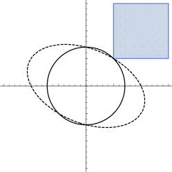
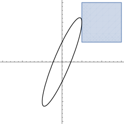
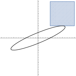
Figure 1: Contours of $\bm{x}^{\top}\bm{\Sigma}^{-1}\bm{x}$ for example $\bm{\Sigma}$ which: (a) satisfy the Savage condition (i.e., $\bm{\Sigma}^{-1}\bm{1}>\bm{0}$), and (b)–(c) do not satisfy the condition. The covariance matrices, in Matlab notation, are: (a) $\bm{\Sigma}=\bm{I}$ and $\bm{\Sigma}=[2,-1/2;-1/2,1]$, (b) $\bm{\Sigma}=[1,2;2,5]$, and (c) $\bm{\Sigma}=[5,2;2,1]$.

A.2 Asymptotic properties of type I elliptical distributions

Take $\bm{X}\sim\mathcal{ELL}(\bm{\mu},\bm{\Sigma},F)$ where the radial distribution $F\in$ MDA(Gumbel) has support $(0,x_{F})$, for some $x_{F}\in\overline{{\mathbb{R}}}$, and where $\{\sigma_{1},\dots,\sigma_{d}\}$ are in decreasing order. The univariate and bivariate asymptotics, $\operatorname{{\mathbb{P}}}(X_{i}>\gamma)$ and $\operatorname{{\mathbb{P}}}(X_{i}>\gamma,X_{j}>\gamma)$, can be written in terms of the scaling function $w(\gamma)$ and of $\mkern 1.0mu\overline{\mkern-1.0mu{F}\mkern 1.25mu}((\gamma-\mu)/\kappa)$ for some particular $\mu$ and $\kappa$. Theorem 12.3.1 of Berman berman1992sojourns gives the univariate case,

$$\operatorname{{\mathbb{P}}}(X_{i}>\gamma)=(1+{\mathrm{o}}(1))\frac{\mkern 1.0mu\overline{\mkern-1.0mu{F}\mkern 1.25mu}(\upsilon_{i}(\gamma))}{\sqrt{2\pi\upsilon_{i}(\gamma)w(\upsilon_{i}(\gamma))}}\quad\text{ as }\gamma\to x_{F}$$ (33)

where $\upsilon_{i}(\gamma)=(\gamma-\mu_{i})/\sigma_{i}$. The bivariate case, i.e. $\operatorname{{\mathbb{P}}}(X_{i}>\gamma,X_{j}>\gamma)$, relies on the following constants. Define $a_{ij}:=\sigma_{j}/\sigma_{i}$. If $\rho_{ij}\geq a_{ij}$ then define

$$\mu_{ij}:=\mu_{j}\quad\text{ and }\quad\kappa_{ij}:=\sigma_{j}$$

otherwise for $\rho_{ij}<a_{ij}$

$$\mu_{ij}:=\frac{\mu_{i}-a_{ij}\rho_{ij}(\mu_{1}+\mu_{2})+a^{2}\mu_{j}}{\alpha_{ij}(1-\rho^{2}_{ij})}\quad\text{ and }\quad\kappa_{ij}:=\frac{\sigma_{i}^{2}\sigma_{j}^{2}(1-\rho^{2}_{ij})}{{\sigma_{i}^{2}-2\rho_{ij}\sigma_{i}\sigma_{j}+\sigma_{j}^{2}}}.$$

Theorem 3

Let $(X_{i},X_{j})$ be a pair from a type I elliptical random vector $\bm{X}\sim E(\bm{\mu},\bm{\Sigma},F)$ and consider $\gamma\nearrow x_{F}$. Then with $\upsilon_{ij}(\gamma)=(\gamma-\mu_{ij})/\kappa_{ij}+c_{ij}(\gamma)$ for some $c_{ij}(\gamma)\in{\mathrm{o}}(1)$,

$$\operatorname{{\mathbb{P}}}(X_{i}>\gamma,X_{j}>\gamma) =\mkern 1.0mu\overline{\mkern-1.0mu{F}\mkern 1.25mu}(\upsilon_{ij}(\gamma))\times\begin{cases}\Big{(}2\pi\upsilon_{ij}(\gamma)w(\upsilon_{ij}(\gamma))\Big{)}^{-1/2}(1+{\mathrm{o}}(1)),&\text{ if }\rho_{ij}>a_{ij},\\ \Big{(}2\pi\upsilon_{ij}(\gamma)w(\upsilon_{ij}(\gamma))\Big{)}^{-1}(C_{a,\rho}+{\mathrm{o}}(1)),&\text{ if }\rho_{ij}<a_{ij},\end{cases}$$

for a $C_{a,\rho}\in{\mathbb{R}}_{+}$. Furthermore, if either $\mu_{i}\geq\mu_{j}$ or $\lim_{\gamma\to x_{F}}w(\gamma)/\gamma<\infty$, then there exists a $C_{\rho}\in{\mathbb{R}}_{+}$ such that

$$\operatorname{{\mathbb{P}}}(X_{i}>\gamma,X_{j}>\gamma) =\mkern 1.0mu\overline{\mkern-1.0mu{F}\mkern 1.25mu}(\upsilon_{ij}(\gamma))\Big{(}2\pi\upsilon_{ij}(\gamma)w(\upsilon_{ij}(\gamma))\Big{)}^{-1/2}(C_{\rho}+{\mathrm{o}}(1)), \text{ if }\rho_{ij}=a_{ij}.$$

Proof

Use Theorem 2 of Hashorva hashorva2007asymptotic . First we consider the case $a_{ij}<\rho_{ij}$. In such a case it holds that

$$\lim_{\gamma\to x_{F}}\sqrt{\frac{w(\upsilon_{j}(\gamma))}{\upsilon_{j}(\gamma)}}\left(\upsilon_{i}(\gamma)-\rho_{ij}\upsilon_{j}(\gamma)\right) =\lim_{\gamma\to x_{F}}\sqrt{{w(\upsilon_{j}(\gamma))\upsilon_{j}(\gamma)}}\left(\frac{\upsilon_{i}(\gamma)}{\upsilon_{j}(\gamma)}-\rho_{ij}\right)$$

$$=\lim_{\gamma\to x_{F}}\sqrt{{w(\upsilon_{j}(\gamma))\upsilon_{j}(\gamma)}}\left(a_{ij}-\rho_{ij}\right)=-\infty.$$

Hence, the hypotheses of Case i) of Theorem 2 of Hashorva hashorva2007asymptotic hold and the first result follows. In the case where $a_{ij}=\rho_{ij}$ then

$$\lim_{\gamma\to x_{F}}\sqrt{\frac{w(\upsilon_{j}(\gamma))}{\upsilon_{j}(\gamma)}}\left(\upsilon_{i}(\gamma)-\rho_{ij}\upsilon_{j}(\gamma)\right)=\lim_{\gamma\to x_{F}}\sqrt{\frac{w(\upsilon_{j}(\gamma))}{\upsilon_{j}(\gamma)}}\frac{(\mu_{j}-\mu_{i})}{\sigma_{i}}.$$

The last limit remains bounded from above if either $\mu_{i}>\mu_{j}$ or $\lim_{\gamma\to\infty}w(\gamma)/\gamma<\infty$. For the case $a_{ij}>\rho_{ij}$ we define $a_{ij}(\gamma):=\upsilon_{i}(\gamma)/\upsilon_{j}(\gamma)$ so $\lim_{\gamma\to\infty}a_{ij}(\gamma)=a_{ij}$.

We let

$$\tau_{ij}(\gamma)=\sqrt{\frac{1-2a_{ij}(\gamma)\rho_{ij}+a_{ij}^{2}(\gamma)}{1-\rho^{2}_{ij}}},\quad\tau_{ij}:=\lim_{\gamma\to\infty}\tau_{ij}(\gamma)=\sqrt{\frac{1-2a_{ij}\rho_{ij}+a_{ij}^{2}}{1-\rho^{2}_{ij}}}.$$

The results follows by noting that

$$\upsilon_{j}(\gamma)\tau_{ij}(\gamma)=\upsilon_{ij}(\gamma),\qquad\upsilon_{ij}(\gamma)=\frac{\gamma-\mu_{ij}}{\tau_{ij}}+{\mathrm{o}}(1).$$

∎

References

- (1) Adler, R.J.: An Introduction to Continuity, Extrema, and Related Topics for General Gaussian Processes. Lecture Notes-Monograph Series 12, i–155 (1990)
- (2) Adler, R.J., Blanchet, J.H., Liu, J., et al.: Efficient Monte Carlo for high excursions of Gaussian random fields. The Annals of Applied Probability 22(3), 1167–1214 (2012)
- (3) Andersen, L.N., Laub, P.J., Rojas-Nandayapa, L.: Online accompaniment for “Efficient simulation for dependent rare events with applications to extremes” (2016). Available at https://github.com/Pat-Laub/RareMaxima
- (4) Anderson, T.W.: An Introduction to Multivariate Statistical Analysis, second edn. Wiley Series in Probability and Mathematical Statistics: Probability and Mathematical Statistics. John Wiley & Sons, Inc., New York (1984)
- (5) Anderson, T.W.: An Introduction to Multivariate Statistical Analysis, third edn. Wiley Series in Probability and Statistics. Wiley-Interscience [John Wiley & Sons], Hoboken, NJ (2003)
- (6) Asmussen, S., Albrecher, H.: Ruin Probabilities, second edn. Advanced Series on Statistical Science & Applied Probability, 14. World Scientific Publishing Co. Pte. Ltd., Hackensack, NJ (2010). DOI 10.1142/9789814282536. URL http://dx.doi.org/10.1142/9789814282536
- (7) Asmussen, S., Glynn, P.W.: Stochastic Simulation: Algorithms and Analysis, Stochastic Modelling and Applied Probability series, vol. 57. Springer (2007)
- (8) Berman, S.: Sojourns and Extremes of Stochastic Processes. CRC Press (1992)
- (9) Bingham, N.H., Goldie, C.M., Teugels, J.L.: Regular Variation, vol. 27. Cambridge university press (1989)
- (10) Botev, Z.I.: The normal law under linear restrictions: Simulation and estimation via minimax tilting. Journal of the Royal Statistical Society, Series B 79, pp. 1–24
- (11) Breslaw, J.: Random sampling from a truncated multivariate normal distribution. Applied Mathematics Letters 7(1), 1–6 (1994)
- (12) Bryc, W.: The Normal Distribution: Characterizations with Applications, vol. 100. Springer Science & Business Media (2012)
- (13) Charpentier, A., Segers, J.: Tails of multivariate Archimedean copulas. Journal of Multivariate Analysis 100(7), 1521–1537 (2009)
- (14) Cont, R.: Encyclopedia of Quantitative Finance (2010)
- (15) De Haan, L., Ferreira, A.: Extreme Value Theory: An Introduction. Springer Science & Business Media (2007)
- (16) Eltoft, T., Kim, T., Lee, T.W.: On the multivariate Laplace distribution. IEEE Signal Processing Letters 13(5), 300–303 (2006)
- (17) Glasserman, P.: Monte Carlo Methods in Financial Engineering, Stochastic Modelling and Applied Probability series, vol. 53. Springer (2003)
- (18) Hashorva, E.: Asymptotics and bounds for multivariate Gaussian tails. Journal of Theoretical Probability 18(1), 79–97 (2005)
- (19) Hashorva, E.: Asymptotic properties of type I elliptical random vectors. Extremes 10(4), 175–206 (2007)
- (20) Hashorva, E.: On the residual dependence index of elliptical distributions. Statistics & Probability Letters 80(13), 1070–1078 (2010)
- (21) Heffernan, J.E.: A directory of coefficients of tail dependence. Extremes 3(3), 279–290 (2000)
- (22) Huang, Z., Shahabuddin, P.: Rare-event, heavy-tailed simulations using hazard function transformations, with applications to value-at-risk. In: Proceedings of the 2003 Winter Simulation Conference, 2003. (2003)
- (23) Hult, H., Lindskog, F., et al.: Multivariate extremes, aggregation and dependence in elliptical distributions. Advances in Applied Probability 34(3), 587–608 (2002)
- (24) Joe, H.: Multivariate Models and Multivariate Dependence Concepts. CRC Press (1997)
- (25) Kotz, S., Kozubowski, T.J., Podgórski, K.: Asymmetric multivariate Laplace distribution. In: The Laplace Distribution and Generalizations, pp. 239–272. Springer (2001)
- (26) Ledford, A.W., Tawn, J.A.: Statistics for near independence in multivariate extreme values. Biometrika 83(1), 169–187 (1996)
- (27) Ledford, A.W., Tawn, J.A.: Modelling dependence within joint tail regions. Journal of the Royal Statistical Society: Series B (Statistical Methodology) 59(2), 475–499 (1997)
- (28) Ledford, A.W., Tawn, J.A., et al.: Concomitant tail behaviour for extremes. Advances in Applied Probability 30(1), 197–215 (1998)
- (29) McNeil, A.J., Frey, R., Embrechts, P.: Quantitative Risk Management: Concepts, Techniques and Tools, 2nd edn. Princeton University Press (2015)
- (30) Nelsen, R.B.: An Introduction to Copulas, 2nd edn. Springer Science & Business Media (2007)
- (31) Nolde, N.: Geometric interpretation of the residual dependence coefficient. Journal of Multivariate Analysis 123, 85–95 (2014)
- (32) Rausand, M., Høyland, A.: System Reliability Theory: Models, Statistical Methods, and Applications, vol. 396. John Wiley & Sons (2004)
- (33) Resnick, S.: Hidden regular variation, second order regular variation and asymptotic independence. Extremes 5(4), 303–336 (2002)
- (34) Resnick, S.I.: Extreme Values, Regular Variation, and Point Processes. Springer (1987)
- (35) Robert, C.P.: Simulation of truncated normal variables. Statistics and computing 5(2), 121–125 (1995)
- (36) Rubinstein, R.Y., Kroese, D.P.: Simulation and the Monte Carlo method, vol. 707. John Wiley & Sons (2011)
- (37) Savage, I.R.: Mills’ ratio for multivariate normal distributions. J. Res. Nat. Bur. Standards Sect. B 66, 93–96 (1962)
- (38) Sibuya, M.: Bivariate extreme statistics. Annals of the Institute of Statistical Mathematics 11(2), 195–210 (1960)