Holographic superconductor with momentum relaxation and Weyl correction

Abstract

We construct a holographic model with Weyl corrections in five dimensional spacetime. In particular, we introduce a coupling term between the axion fields and the Maxwell field such that the momentum is relaxed even in the probe limit in this model. We investigate the Drude behavior of the optical conductivity in low frequency region. It is interesting to find that the incoherent part of the conductivity is suppressed with the increase of the axion parameter $k/T$, which is in contrast to other holographic axionic models at finite density. Furthermore, we study the superconductivity associated with the condensation of a complex scalar field and evaluate the critical temperature for condensation in both analytical and numerical manner. It turns out that the critical temperature decreases with $\tilde{k}$, indicating that the condensation becomes harder in the presence of the axions, while it increases with Weyl parameter $\gamma$. We also discuss the change of the gap in optical conductivity with coupling parameters. Finally, we evaluate the charge density of the superfluid in zero temperature limit, and find that it exhibits a linear relation with $\tilde{\sigma}_{DC}(\tilde{T_{c}})\tilde{T_{c}}$, such that a modified version of Homes’ law is testified.

I Introduction

The high $T_{c}$ superconductivity in some novel materials such as Cuprates and heavy Fermion compounds involves the strong couplings of electrons, thus beyond the traditional BCS theory which describes the electron-phonon interaction very well. Recent progress in the AdS/CMT duality has provided powerful tools for understanding novel phenomena in strongly coupled system Hartnoll:2008vx ; McGreevy:2009xe ; Herzog:2009xv ; Iqbal:2011ae ; Hartnoll:2008kx ; Gubser:2008px ; Horowitz:2010gk ; Hartnoll:2009sz . Especially, a holographic description of the condensation was originally proposed in Gubser:2008px by Gubser and a holographic model for the superconductor was firstly constructed in Hartnoll:2008vx ; Hartnoll:2008kx by Hartnoll, Herzog and Horowitz. One key ingredient in this holographic model is introducing the spontaneous breaking of $U(1)$ gauge symmetry in the bulk geometry, which is analogous to the mechanism of s-wave superconductors. We refer to Refs. Horowitz:2010gk ; Hartnoll:2009sz ; Cai:2015cya for a comprehensive review on holographic superconductors.

It is very interesting to enrich the holographic setup to investigate various novel phenomena observed in condensed matter experiments. For instance, a Weyl term composed of the couplings of the Weyl tensor and the Maxwell field was introduced in Ritz:2008kh ; Myers:2010pk and then has extensively been investigated in holographic literature Sachdev:2011wg ; Wu:2010vr ; Momeni:2011ca ; WitczakKrempa:2012gn ; WitczakKrempa:2013ht ; Witczak-Krempa:2013aea ; Witczak-Krempa:2013nua ; Katz:2014rla ; Ling:2016dck ; Wu:2016jjd . Since the self duality of the Maxwell field is violated due to the presence of the Weyl term, it provides a novel mechanism for understanding the condensed matter phenomena with the breakdown of the electromagnetic self-duality from a holographic perspective. Historically, this model also provides a way of turning on a nontrivial frequency dependence for the optical conductivity of the dual QFT, which has been studied with small parameter perturbation theory as well as the variational method in Myers:2010pk ; Sachdev:2011wg ; Wu:2010vr ; Momeni:2011ca ; WitczakKrempa:2012gn . However, to obtain a finite DC conductivity over a charged black bole background, one essential step is to break the translational invariance such that the momentum is not conserved. Until now there are many ways to introduce the momentum relaxation or momentum dissipation in holographic approach. It can be implemented by spatially periodic sources Horowitz:2012ky ; Horowitz:2012gs ; Horowitz:2013jaa ; Ling:2013aya ; Ling:2013nxa ; Ling:2014saa , helical and Q-lattices Donos:2012js ; Donos:2014oha ; Donos:2013eha ; Donos:2014uba ; Ling:2014laa , spatially linear dependent axions Andrade:2013gsa ; Gouteraux:2014hca ; Kim:2014bza ; Cheng:2014qia ; Ge:2014aza ; Mozaffara:2016iwm , or massive gravitonsdeRham:2010kj ; Hassan:2011hr ; Vegh:2013sk ; Blake:2013bqa ; Blake:2013owa ; Davison:2013jba (for a brief review we refer to Ref.Ling:2015ghh ). In the presence of slow momentum relaxation, it is found that the optical conductivity exhibits a Drude behavior in the low frequency region, which has become a widespread phenomenon in holographic models. However, when the momentum relaxation becomes strong, the discrepancy from the Drude formula can be observed even in the low frequency region, leading to the incoherence of the conductivity. Currently, it is still a crucial issue to understand the coherent/incohenrent behavior of metal in both condensed matter physics and holographic gravity Kim:2014bza ; Ge:2014aza ; Hartnoll:2014lpa ; Davison:2014lua ; Davison:2015bea ; Davison:2015taa ; Zhou:2015qui .

In this paper we intend to construct a holographic model with momentum relaxation in the presence of the Weyl term. Moreover, inspired by recent work in Gouteraux:2016wxj , we intend to provide a novel scheme to introduce the momentum relaxation by considering the coupling between the axions and the Maxwell field. In this way we could consider the coherence/incoherence of the metal even in the probe limit where the charge density is vanishing in the background. In contrast to usual holographic models with axions where the incoherence of the conductivity becomes manifest when the momentum relaxation becomes strong, we find in our model the portion of incoherent conductivity is suppressed with the increase of the axion parameter $k/T$.

In the second part of this paper we will construct a holographic model for s-wave superconductor by the spontaneous breaking of $U(1)$ gauge symmetry. We will investigate the condensation of the complex scalar field and evaluate the critical temperature as well as the energy gap which may vary with the strength of the momentum relaxation. Another motivation of our current work is to testify the Homes’ law in the holographic perspective. In condensed matter literature Homes2004 ; Homes2005 , it has been shown by experiments that for a large class of superconductivity materials there exists an elegant empirical law linking the charge density of superfluid at zero temperature to the $DC$ conductivity near the critical temperature, which now is dubbed as Homes’ law. This law discloses that regardless of the structure of materials, the superconductivity always exhibits a universal behavior as

$$\rho_{s}(T=0)=C\sigma_{DC}(T_{c})T_{c},$$ (1)

where the constant $C$ is found to be about $4.4$ for in-plane high-$T_{c}$ superconductors and clean BCS superconductors, while for $c$-axis high-$T_{c}$ materials and BCS superconductors in dirty limit $C=8.1$. For organic superconductors the $C=4\pm 2.1$ Homes2013 . On the theoretical side, a preliminary understanding on the Homes’ law of high-$T_{c}$ superconductors was proposed with the use of the notion of Planckian dissipator in Zaanen2004 . However, for the conventional superconductors which are subject to the Homes’ law as well, a corresponding interpretation in theory is still missing. An alternative mechanism with double timescales proposed to understand Homes’ law can also be found in Phillips2005 . Nevertheless, people believe that the present stage is still far from a complete understanding on the Homes’ law in theory. In particular, for high temperature superconductivity, it is believed that the BCS theory breaks down and some novel techniques should be developed to treat the many-body system which is strongly coupled. Holography has rendered us a powerful tool to address such an open problem. Therefore, recently it has been becoming very intriguing to testify if the Homes’ law would be observed in holographic approach. Earlier attempts in this route can be found in Erdmenger:2012ik ; Erdmenger:2015qqa ; Kim:2016hzi ; Kim:2016jjk . In this paper we intend to demonstrate that a modified Homes’ law can be observed in our model as well.

This paper is organized as follows. The holographic setup of our model is given in section II. Then we investigate the electric transport properties of the dual field theory in section III, focusing on the coherent-incoherent transition with the strength of axions. In section IV we turn to the superconductivity of this model. The critical temperature for condensation and the energy gap are evaluated. Particularly, we will focus on the test of Homes’ law based on the transport properties of the superconductivity. Some open questions and possible development are discussed in section V. As a byproduct, we present an efficient way to get rid of the effects due to the presence of nonanalytic terms in numerical simulation in the Appendix.

II Holographic Setup

The holographic superconductors with momentum relaxation and dissipation have been investigated in various models, such as Horowitz:2013jaa ; Ling:2014laa ; Andrade:2014xca ; Erdmenger:2015qqa ; Kim:2016hzi ; Kim:2016jjk ; Kim:2015dna ; Baggioli:2015zoa . Here we consider a holographic model in Einstein-Maxwell-Axion theory with a Weyl correction in five dimensional spacetime. The total Lagrangian is given by Gouteraux:2016wxj ; Baggioli:2016oqk

$$\mathcal{L}=R+\frac{12}{L^{2}}-\frac{1}{4}\left(1+\mathcal{K}Tr[X]\right)F^{2}-{\left|\nabla\psi-ieA\psi\right|}^{2}-m^{2}{\left|\psi\right|}^{2}+{\gamma}L^{2}C_{\mu\nu\rho\sigma}F^{\mu\nu}F^{\rho\sigma},$$ (2)

where $X^{\mu}_{\nu}=\frac{1}{3}g^{\mu\tau}\partial_{\tau}{X^{I}}\partial_{\nu}{X^{I}}$ with ${X^{I}}$ being axion fields, which constitute massive term of graviton. $C_{\mu\nu\rho\sigma}$ is the Weyl tensor which is coupled to the Maxwell field with a coupling parameter $\gamma$. In this action we have also introduced a coupling term between the axions and Maxwell fields as proposed in Gouteraux:2016wxj . Following the analysis in Gouteraux:2016wxj , we will set the coupling constant $\mathcal{K}=\frac{1}{7}$ throughout this paper. In addition, from Ritz:2008kh we know the value of $\gamma$ has to obey the following constraint for the sake of causality and stability of the system

$$-\frac{L^{2}}{16}<\gamma<\frac{L^{2}}{24}.$$ (3)

Furthermore, for simplicity we set $m^{2}=-\frac{3}{L^{2}}$ and $L=1$.

In the presence of the Weyl correction, usually it is very hard to obtain the analytical solutions with backreaction, although the approximate solution could be obtained when the Weyl parameter is very smallLing:2016dck . In current paper we will only consider the probe limit of the system. That is to say, the gravity is decoupled from the matter fields. We fix the background as an AdS-Schwarzschild black brane whose metric reads as

$$ds^{2}=\frac{{r_{H}}^{2}}{z^{2}}\left(-f(z)dt^{2}+dx^{2}+dy^{2}+dw^{2}\right)+\frac{dz^{2}}{z^{2}f(z)},$$ (4)

where $f(z)=1-z^{4}$ with $0<z<1$. $r_{H}$ is the position of the black hole horizon and we will set it as unit in numerics throughout this paper. The Hawking temperature of the black hole is given as $T=\frac{r_{H}}{\pi}$.

III Conductivity in normal phase

In this section we will investigate the electrical transport behavior of the dual field theory without condensation, namely $\psi=0$. Firstly, it is easy to see that $X^{I}=k\delta^{I}_{i}x^{i}$, with $i$ running over boundary space indices, is a solution to the equations of motion for axion fields. We will consider the conductivity of the gauge field in one spatial direction, say x-direction, over such a background with momentum relaxation. In the absence of the condensation, the $x$-component of the gauge field is decoupled from other fields except axions $X^{I}$ and thus we can only turn on the electric field in this direction. Consider a perturbation with a form $A_{x}(z)e^{i\omega t}$ in linear response theory, we have a single perturbation equation as

$$A_{x}^{\prime\prime}(z)+\left(\frac{3}{z}+\frac{g^{\prime}(z)}{g(z)}+\frac{2\left(\gamma z^{5}g^{(3)}(z)+6\gamma z^{4}g^{\prime\prime}(z)+6\gamma z^{3}g^{\prime}(z)+3\right)}{zh(z)}\right)A_{x}^{\prime}(z)$$ (5)

$$+\frac{\omega^{2}}{z^{4}g(z)^{2}}A_{x}(z)=0$$

where $h(z)=2\gamma z^{4}g^{\prime\prime}(z)+8\gamma z^{3}g^{\prime}(z)+4\gamma z^{2}g(z)-3\mathcal{K}k^{2}z^{2}-3$. Notice that in five dimensional space time, ${A_{x}}(z)$ has the following asymptotical behavior at spatial infinity $z=0$

$$A_{x}(z)=A_{x}^{0}+A_{x}^{2}{z^{2}}-\frac{\left(\omega^{2}A_{x}^{0}\right)\log\left(\frac{z}{\Lambda}\right){z^{2}}}{2},$$ (6)

where $\Lambda$ is an arbitrary constant. The logarithmic divergency can be removed by introducing a counterterm, which is Taylor:2000xw ; Horowitz:2012gs

$$S_{ct}=\frac{L\log(\nu z)}{4}\int\sqrt{-\gamma}F^{2}\,dx^{4}.$$ (7)

Then following the standard holographic dictionary, we may obtain the optical conductivity for the dual field theory as

$$\sigma(\omega)=\frac{1}{iL^{3}\omega}\left(\frac{2A_{x}^{2}}{A_{x}^{0}}+\omega^{2}\left(\log\left(\frac{\Lambda}{\nu}\right)-\frac{1}{2}\right)\right).$$ (8)

Usually, the non-analytic behavior caused by the logarithmic term brings some difficulties to guarantee the convergency in numerical calculation and it becomes harder for one to extract the data for the coefficients in the expansion (6) with enough accuracy. Alternatively, we find that it is more numerically efficient to replace $A_{x}(z)$ by $(1-z)^{\frac{-i\omega}{4}}\left(a_{x}(z)-\frac{1}{2}\omega^{2}A_{x}^{0}\frac{\log(z)z^{2}}{2}\right)$ in perturbation equation (5), then the equation for $a_{x}(z)$ is analytic everywhere and the conductivity can be reexpressed in terms of $a_{x}(z)$ as

$$\sigma(\omega)=\frac{1}{iL^{3}\omega}\left(\frac{a_{x}^{{}^{\prime\prime}}(z\to 0)}{a_{x}(z\to 0)}+\omega^{2}\left(\log\left(\frac{\Lambda}{\nu}\right)-\frac{1}{2}\right)+\frac{\omega^{2}}{16}+\frac{i\omega}{4}\right).$$ (9)

The derivation from (8) to (9) is presented in Appendix.

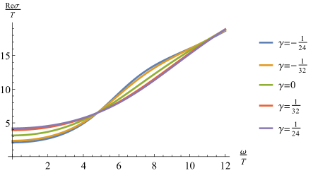
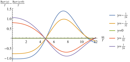
Figure 1: The real part of the conductivity for different values of $\gamma$ with $k=0$.

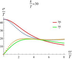
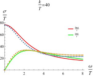
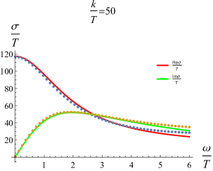
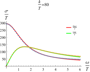
Figure 2: The frequency dependence of conductivity for $k/T=30,40,50,$ and $80$ respectively with $\gamma=0$. Dotted lines are numerical data, while solid lines are fit with the modified Drude formula $\sigma(\omega)=\frac{K\tau}{1-i\omega\tau}+\sigma_{Q}$.

Next we intend to demonstrate our numerical results for the optical conductivity based on Eq.(9) in the case of $\log\left(\frac{\Lambda}{\nu}\right)=0$.

• $k=0,\gamma\neq 0$. It is very interesting to notice that both the axion parameter $k$ and Weyl parameter $\gamma$ appear in the same term in the perturbation equation, as shown in (5), implying that the momentum relaxation and the Weyl correction play a similar role in influencing the optical conductivity. Firstly, we illustrate the frequency behavior of the real part of the conductivity for various values of $\gamma$ with $k=0$, as plotted in Figure.1. It is nothing but the extension of the results in four dimensions presented in Myers:2010pk to five dimensions. For zero frequency region, we observe the similar phenomena as disclosed in Myers:2010pk . Namely, the DC conductivity increases with $\gamma$. Quantitatively, our numerical result of $\sigma_{DC}$ agrees with the analytical result which is $\sigma_{DC}/T=(1+8\gamma)/T=\pi(1+8\gamma)$ Ritz:2008kh . While for large frequency region, the conductivity becomes independent of the value of $\gamma$, and always has a linear relation with the frequency rather than a constant as in four-dimensional case. This is a reflection of the different dimensions of the boundary geometryMyers:2010pk ; Wu:2016jjd ; WitczakKrempa:2012gn . Furthermore, if one subtracts the conductivity with $\gamma=0$, a peak (for $\gamma>0$) or a dip (for $\gamma<0$) can obviously be observed near the zero frequency region, as illustrated in the bottom plot of Fig.1, which is similar to the phenomenon in four dimensions. Interestingly, for small $\gamma$ region, it seems there exists a mirror symmetry around the horizontal axis if one changes $\gamma$ to $-\gamma$, which has previously been discussed in Myers:2010pk ; WitczakKrempa:2012gn ; WitczakKrempa:2013ht ; Witczak-Krempa:2013aea ; Witczak-Krempa:2013nua ; Ling:2016dck . Furthermore, since the value of $\gamma$ is subject to the constraint in (3), we find the Weyl term has limited impact on the conductivity. Specially, a Drude behavior in low frequency region can not be observed. However, if one ignores the restriction in (3), a Drude peak would emerge when $\gamma\gg 1$, as discussed in Wu:2016jjd . This is not surprising as we have pointed out that the axion parameter $k$ and Weyl parameter $\gamma$ do play similar roles in the perturbation equation. Finally, we remark that if one introduces some other Weyl terms with higher derivatives, then the additional coefficients involved may not be bounded as $\gamma$ such that a substantial Drude-like peak at small frequencies can be achieved as well by adjusting these coefficients, as discussed in Witczak-Krempa:2013aea .

• $k\neq 0,\gamma=0$. In this case the Weyl curvature term is vanished while the momentum is relaxed. Firstly, for $\omega=0$, the real part of numerical conductivity is increasing with $k/T$, which is consistent with the analytical result in Gouteraux:2016wxj . Secondly, we find a prominent Drude-like peak in low frequency region of the optical conductivity, as shown in FIG.2. Numerically, we also find that when $k/T$ becomes large, the $\sigma_{DC}$ is increasing and the numerical data can be fit well with a modified Drude formula, namely, $\sigma(\omega)=\frac{K\tau}{1-i\omega\tau}+\sigma_{Q}$, where $\sigma_{Q}$ is a real constant signalizing the incoherent contribution to the conductivity. To quantitatively measure the incoherent contribution to the total conductivity, we intend to define a quantity $\sigma_{Q}/(K\tau)$ and plot its variation with the momentum relaxation $k/T$, which is shown in the left plot of Fig.3. Interestingly enough, we find the portion of incoherent contribution is decreasing with the increase of $k/T$. It indicates that the metallic phase of the dual system looks more coherent in large $k/T$ region indeed. Such behavior is in contrast to the phenomenon observed in most previous holographic models with axions, where a Drude-like peak can be observed even with small $k/T$ and the incoherence of the metal becomes evident in large $k/T$ region Kim:2014bza ; Wu:2016jjd ; Ge:2014aza . First of all. In usual lattice models or axion models, the backreaction of lattice to the background is taken into account such that the translational invariance is broken already prior to the linear perturbations. Technically, the chemical potential $\mu$ contributes a term $\mu^{2}/k^{2}$ in the usual expression for the DC conductivity, leading to a prominent Drude peak even if the lattice effect is weak (with tiny $k/T$). However, in our paper, only the neutral background is taken into account under the probe limit such that the effect of this term is absent. More importantly, the difference results from the different coupling manner of axion and Maxwell field. In our model the axion fields do not contribute any independent terms such as the kinematic term or potential term in the Lagrangian (2). It only appears as a term coupled to Maxwell field such that it induces the momentum relaxation only at the linear response level. In hence, the Drude behavior would not become manifest until the momentum relaxation becomes strong with the axion parameter $k/T$. Moreover, the coupling term plays a double role in influencing the transport behavior. One is to control the generation of electron-hole pairs which roughly speaking is responsible for the incoherent part of conductivity, reflected by the quantity $\sigma_{Q}$. The other one is to induce the momentum relaxation, leading to coherent conductivity, reflected by the quantity $K\tau$ Gouteraux:2016wxj . With the increase of $k/T$ both quantities $\sigma_{Q}$ and $K\tau$ increase, while as a result of competition, the ratio $\sigma_{Q}/(K\tau)$ becomes smaller with larger $k/T$. As a matter of fact, the enhancement of the coherence can also be perceived if one evaluates the relaxation time for different $k/T$. Our results indicate that it increases with $k/T$, as shown in the left plot of FIG.4.

  

  

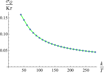
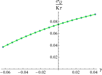
  Figure 3: The ratio of incoherent part to the coherent part in $DC$ conductivity. The left plot is for varying $k/T$ with $\gamma=0$, while the right plot is for varying $\gamma$ with $k/T=25$

  .

• $k\neq 0,\gamma\neq 0$. In this case the translational invariance is broken. The optical conductivity has a similar behavior as in above case when changing $k/T$ with $\gamma$ fixed, since the Weyl parameter is constrained to take values in a small region. On the other hand, if we change $\gamma$ with $k/T$ fixed, we find that the ratio of the incoherent conductivity to the coherent part increases with $\gamma$, as illustrated in the right plot of FIG.3. In addition, our data indicate that the relaxation time is linear with $\gamma$, and our fitted result is $\tau T=0.463\gamma+0.238$, which is shown in the right plot of FIG.4.

  

  

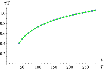
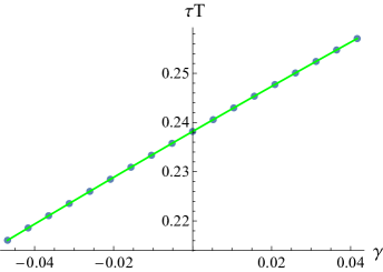
  Figure 4: The relation between the relaxation time $\tau T$ and the system parameters $k/T$ and $\gamma$. The left plot is for varying $k/T$ with $\gamma=0$, while the right plot is for varying $\gamma$ with $k/T=25$.

IV Conductivity in superconducting phase

In the remainder of this paper we turn to investigate the transport properties of the superconducting phase in this model. We will turn on the complex scalar field and introduce the spontaneous breaking of $U(1)$ gauge symmetry. In probe limit, the system becomes simple and we intend to firstly evaluate the critical temperature for the condensate in an analytical way, and then compute the frequency behavior of the conductivity with numerical analysis, focusing on the evaluation of the energy gap and the test of Homes’ law.

IV.1 Analytical part

In this subsection we will evaluate the critical temperature for condensation closely following the procedures of matching method as given in literature Gregory:2009fj ; Kuang:2010jc ; Roychowdhury:2012hp . The basic idea is to find an approximate solution to the equations of condensate by virtue of series expansion. We expand all the variables near the boundary $z=0$ and the horizon $z=1$ separately which are subject to the equations of motion, then require these series expansion of the same variable is matched at some intermediate location, for instance $z=\frac{1}{2}$.

IV.1.1 Expansion near the boundary and horizon

After turning on the complex scalar field, the Lagrangian of the matter part is given by

$${\mathcal{L}}_{2}=-\frac{1}{4}\left(1+\mathcal{K}Tr[X]\right)F^{2}-{\left|\nabla\psi-ieA\psi\right|}^{2}-m^{2}{\left|\psi\right|}^{2}+{\gamma}L^{2}C_{\mu\nu\rho\sigma}F^{\mu\nu}F^{\rho\sigma}.$$ (10)

With the ansatz $A_{\mu}=(a(z),0,0,0,0)$, we derive the equations of motion as follows

$$a^{\prime\prime}(z)+\left(\frac{2\left(\gamma z^{5}g^{(3)}(z)+6\gamma z^{4}g^{\prime\prime}(z)+6\gamma z^{3}g^{\prime}(z)-{r_{H}}^{2}\right)}{ze(z)}+\frac{1}{z}\right)a^{\prime}(z)-\frac{2{r_{H}}^{4}\psi(z)^{2}}{z^{4}e(z)g(z)}a(z)=0,$$ (11)

$$\psi^{\prime\prime}(z)+\frac{\psi^{\prime}(z)\left(z^{4}g(z)g^{\prime}(z)-z^{3}g(z)^{2}\right)}{z^{4}g(z)^{2}}+\frac{\psi(z)\left(a(z)^{2}+3g(z)\right)}{z^{4}g(z)^{2}}=0,$$ (12)

$$\nabla_{\mu}\left[\left(\nabla^{\mu}X^{I}\right)F^{2}\right]=0,$$ (13)

where $g(z)=\frac{{r_{H}}^{2}}{z^{2}}\left(1-z^{4}\right)$, $e(z)=2\gamma z^{4}g^{\prime\prime}(z)+8\gamma z^{3}g^{\prime}(z)+4\gamma z^{2}g(z)+\mathcal{K}k^{2}z^{2}+{r_{H}}^{2}$. It is easy to figure out that $X^{I}=k\delta^{I}_{i}x^{i}$ is a solution of the last equation of (13), where $i$ runs over boundary space indices. With the use of EOM, we find the asymptotical behavior of fields at $z=0$, which are

$$a(z)=\mu-qz^{2}+\cdots\qquad\qquad\psi(z)={\psi_{-}}z^{\lambda_{-}}+\cdots+{\psi_{+}}z^{\lambda_{+}}+\cdots,$$ (14)

where $\lambda_{+}=3$, $\lambda_{-}=1$. On the other hand, with the use of EOM we find $a(1)=0$ on the horizon. We require that the Maxwell field and scalar field are regular at horizon, such that we expand $a(z)$ and $\psi(z)$ near horizon as follows

$$a(z)\approx a^{\prime}(1)(z-1)+\frac{1}{2}a^{\prime\prime}(1)(z-1)^{2}+\cdots,$$ (15)

$$\psi(z)\approx\psi(1)+\psi^{\prime}(1)(z-1)+\frac{1}{2}\psi^{\prime\prime}(1)(z-1)^{2}+\cdots.$$ (16)

Next we intend to solve for $a^{\prime\prime}(1)$ and $\psi^{\prime\prime}(1)$ by series expansion of the equations of motion. Substituting $g(z)=\frac{{r_{H}}^{2}}{z^{2}}\left(1-z^{4}\right)$ into the EOM, we obtain

$$a^{\prime\prime}(1)=-\frac{-144{r_{H}}^{2}\gamma+2\mathcal{K}k^{2}+{r_{H}}^{2}\psi^{\prime}(1)^{2}-2{r_{H}}^{2}}{2\left(-24{r_{H}}^{2}\gamma+\mathcal{K}k^{2}+{r_{H}}^{2}\right)}a^{\prime}(1),$$ (17)

$$\psi^{\prime}(1)=\frac{3}{4}\psi(1),$$ (18)

and

$$\psi^{\prime\prime}(1)=-\frac{21}{16}\psi(1)-\frac{a^{\prime}(1)^{2}\psi(1)}{32{r_{H}}^{2}}+\frac{9}{8}\psi^{\prime}(1).$$ (19)

Combining (18) and (19), we have

$$\begin{aligned} \psi^{\prime\prime}(1)=-\frac{15}{32}\psi(1)-\frac{{a^{\prime}(1)^{2}}\psi(1)}{32{r_{H}}^{2}}\end{aligned}.$$ (20)

Finally, inserting (17), (18) and (20) into (15) and (16), we obtain the series expansion of the fields as

$$a(z)\approx a^{\prime}(1)(z-1)-\frac{-144{r_{H}}^{2}\gamma+2\mathcal{K}k^{2}+{r_{H}}^{2}\psi^{\prime}(1)^{2}-2{r_{H}}^{2}}{2\left(-24{r_{H}}^{2}\gamma+\mathcal{K}k^{2}+{r_{H}}^{2}\right)}a^{\prime}(1)(z-1)^{2}+\cdots,$$ (21)

and

$$\psi(z)\approx\psi(1)+\frac{3}{4}\psi(1)(z-1)-\frac{1}{2}\left(\frac{15}{32}\psi(1)+\frac{{a^{\prime}(1)^{2}}\psi(1)}{32{r_{H}}^{2}}\right)(z-1)^{2}+\cdots.$$ (22)

IV.1.2 Matching at $z=\frac{1}{2}$

Matching (14) with (21) and (22) at $z=\frac{1}{2}$, we obtain

$$\psi(1)^{2}=-\frac{2\left(a^{\prime}(1)\left(-120{r_{H}}^{2}\gamma+3\mathcal{K}k^{2}+{r_{H}}^{2}\right)+2q\left(-24{r_{H}}^{2}\gamma+\mathcal{K}k^{2}+{r_{H}}^{2}\right)\right)}{{r_{H}}^{2}a^{\prime}(1)},$$ (23)

and

$$\begin{aligned} a^{\prime}(1)=-\frac{r_{H}\sqrt{145\lambda_{+}-126}}{\sqrt{\lambda_{+}+2}}\end{aligned}.$$ (24)

Furthermore, inserting (24) into (23), we have

$$\psi(1)^{2}=240\gamma-\frac{6\mathcal{K}k^{2}}{{r_{H}}^{2}}-2+\frac{4\sqrt{\lambda+2}q\left(\mathcal{K}k^{2}+(1-24\gamma){r_{H}}^{2}\right)}{\sqrt{145\lambda_{+}-126}{r_{H}^{3}}}.$$ (25)

After replacing $q$ by $\frac{\rho}{{r_{H}}^{2}}$ and $r_{H}$ by $\pi{L^{2}}T$ respectively, we set $\psi(1)^{2}=0$, then the critical temperature for condensation can be estimated by finding the root of the following polynomial equation

$$T^{5}-\frac{3\mathcal{K}k^{2}T^{3}}{\pi^{2}b}+\frac{2(1-24\gamma)\sqrt{\lambda_{+}+2}\rho}{\pi^{3}bc}T^{2}+\frac{2\mathcal{K}k^{2}\sqrt{\lambda_{+}+2}\rho}{\pi^{5}bc}=0,$$ (26)

where $b=120\gamma-1$ and $c=\sqrt{145\lambda_{+}-126}$. For instance, if we set $\gamma=0,\mathcal{K}=\frac{1}{7}$ while change $k/\rho^{1/3}=0,1,2$, we obtain the values of the critical temperature $T/\rho^{1/3}$ as 0.20170, 0.17011, 0.14979, respectively, implying that the condensation becomes harder with the increase of momentum relaxation $k$. Moreover, if we fix for instance $\rho=1,\mathcal{K}=\frac{1}{7},k=1$ but change $\gamma=-\frac{1}{96},0,\frac{1}{124}$, the corresponding values for the critical temperature $T/\rho^{1/3}$ are 0.15534, 0.17011, 0.20854, implying that the increase of the Weyl parameter makes the condensation easier. In next part we will see soon that this trend can be justified by explicitly solving the equations of motion with numerical method.

IV.2 Numerical part

In this part we will explicitly solve the condensation equations with numerical method and demonstrate the parameter dependence of the critical temperature, then we will numerically solve the perturbation equations to compute the optical conductivity along x-direction below the critical temperature. In the remainder of this paper, we will take the charge density as the unit such that all the dimensionless quantities will be denoted with a tilde, namely as $\tilde{O}$. Thus $\tilde{T}$ is the dimensionless temperature $T/\rho^{1/3}$ while $\tilde{T_{c}}$ is $T/\rho_{c}^{1/3}$ and so forth.

• Condensation of the scalar field. First we numerically determine the critical temperature by solving EMO (11) and (12), at which the scalar hair starts to condensate, leading to nontrivial solutions. We solve these equations with the use of the spectral method. As a result, the parameter dependence of the critical temperature is shown in FIG.5. From the left plot we learn that the critical temperature becomes lower with the increase of $\tilde{k}$, but becomes higher with the increase of $\gamma$, which is consistent with FIG.6. These numerical results verify our analytical approximation through the matching method in previous subsection. In the presence of axions, as $\tilde{k}$ becomes larger, the momentum dissipation becomes stronger such that the condensation becomes harder, which is similar to the effects of the Q-lattices as demonstrated in Ling:2014laa but in contrast to the scalar lattices as found in Horowitz:2013jaa . Our result here is also different from the previous superconductor models with axions where the critical temperature may have non-monotonic relation with $\tilde{k}$, for instance in Andrade:2014xca ; Kim:2015dna ; Baggioli:2015zoa . This is simply because only the probe limit is taken into account in our paper. On the other hand, when the Weyl correction is taken into account, as $\gamma$ becomes larger, the generation of electron-like excitations exceeds that of vortex-like excitations such that the condensation of s-wave becomes easier. What we have found for changing $\gamma$ is consistent with the previous results as discussed in Wu:2010vr ; WitczakKrempa:2012gn . However, it is worthwhile to point out that in p-wave model the presence of Weyl term may make the phase transition harder Zhao:2012kp .

  

  

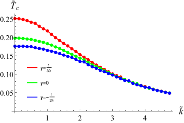
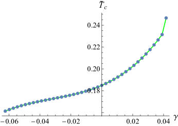
  Figure 5: The variation of the critical temperature with the system parameters. The left plot is $\tilde{T_{c}}$ versus $\tilde{k}$ for various $\gamma$, while the right plot is $\tilde{T_{c}}$ versus $\gamma$ for $\tilde{k}=1$.

  

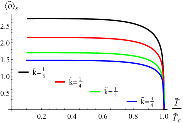
  Figure 6: The condensation of the scalar field below the critical temperature for various $\tilde{k}$ with $\gamma=0$

  .

• The frequency behavior of the optical conductivity and energy gap. Now we consider the transport behavior of the dual system by linear response theory. We first derive the linear perturbation equation for $A_{x}(z,t)=A_{x}(z)e^{i\omega t}$, which reads as

  $$A_{x}^{\prime\prime}(z)+\left(\frac{3}{z}+\frac{g^{\prime}(z)}{g(z)}+\frac{2\left(\gamma z^{5}g^{(3)}(z)+6\gamma z^{4}g^{\prime\prime}(z)+6\gamma z^{3}g^{\prime}(z)+3\right)}{zh(z)}\right)A_{x}^{\prime}(z)$$ (27)

  $$+\left(\frac{6\psi(z)^{2}}{z^{4}g(z)h(z)}+\frac{\omega^{2}}{z^{4}g(z)^{2}}\right)A_{x}(z)=0,$$

  where $h(z)=2\gamma z^{4}g^{\prime\prime}(z)+8\gamma z^{3}g^{\prime}(z)+4\gamma z^{2}g(z)-3\mathcal{K}k^{2}z^{2}-3$. Next we turn on the external electric field along x-direction by imposing appropriate boundary condition at $z=0$. As usual, the ingoing boundary condition is imposed on the horizon. We demonstrate the frequency behavior of the conductivity in Fig.7 and FIG.8 for different values of parameters. First of all, we notice that the imaginary part of the conductivity is divergent in zero frequency limit, indicating a superconducting phase for the dual system. Secondly, we observe that the energy gap shifts with the change of the parameters in our model. Specifically, the energy gap becomes small with the increase of $\tilde{k}$, as illustrated in FIG.7. By locating the minimal value of the imaginary part of the conductivity,

  we find that the energy gap $\tilde{\omega}/\tilde{T}_{c}$ is 8.26, 8.13, 7.88, 7.63 corresponding to $\tilde{k}=\frac{1}{8},\frac{1}{4},\frac{1}{2},\frac{3}{4}$, respectively. On the other hand, the energy gap decreases with $\gamma$, as illustrated in FIG.8, where the value of energy gap runs from $7.51,7.26,7.00$ to $6.26$, corresponding to $\gamma=-\frac{1}{96},0,\frac{1}{96},\frac{1}{32}$, respectively.

  What we have observed above are consistent with the results in Wu:2010vr , but have an opposite tendency in comparison with the results in Gauss-Bonnet gravity and quasi-topological gravity in which the energy gap becomes larger than $8$ with the increase of system parametersPan:2009xa ; Kuang:2010jc .

• A modified Homes’ law. In the presence of the axions , the dual system is a two-fluid system below the critical temperature, composed of the normal fluid and the superfluid. The density of superfluid can be evaluated by $Im(\tilde{\sigma})\sim 2\pi\tilde{\rho}_{s}/\tilde{\omega}$ with extremely low temperature. As a consequence, we may investigate the relation between this quantity and $\tilde{\sigma}_{DC}(\tilde{T_{c}})\tilde{T_{c}}$ by changing system parameters. Some examples have been illustrated by changing $\tilde{k}$ in FIG.9, with $\gamma=-\frac{1}{24},0,\frac{1}{30}$, respectively. From right to left, $\tilde{k}$ runs from 0 to 5 for each value of $\gamma$. We remark that here both $\tilde{\rho}_{s}$ and $\tilde{\sigma}_{DC}(\tilde{T_{c}})\tilde{T_{c}}$ are scaleless quantities. Interestingly enough, a manifest linear relation has been observed for these two quantities, signalizing a Homes’ law for this model. However, our data fitting tells us that the intercept at the vertical axis might not be zero if extending the straight line to $\tilde{\sigma}_{DC}(\tilde{T_{c}})\tilde{T_{c}}=0$. Instead, a modified version of Homes’ law is the best fitting, which is $\tilde{\rho}_{s}=C\tilde{\sigma}_{DC}(\tilde{T_{c}})\tilde{T_{c}}+a$. In this figure for different $\gamma$, we have $\tilde{\rho}_{s}=0.90\tilde{\sigma}_{DC}(\tilde{T_{c}})\tilde{T_{c}}+1.26$, $\tilde{\rho}_{s}=0.94\tilde{\sigma}_{DC}(\tilde{T_{c}})\tilde{T_{c}}+1.23$, $\tilde{\rho}_{s}=0.96\tilde{\sigma}_{DC}(\tilde{T_{c}})\tilde{T_{c}}+1.20$, respectively. It is worthwhile to point out that we are not able to evaluate $\tilde{\rho}_{s}$ at absolute zero temperature numerically. Instead we obtain its value at $\tilde{T}=0.1\tilde{T_{c}}$. This identification should be fine since $\tilde{\rho}_{s}\thicksim\tilde{\langle\mathcal{O}\rangle}$ Hartnoll:2008vx ; Horowitz:2009ij and from Fig.6 we know $\tilde{\rho}_{s}$ is almost saturated to a constant below the critical temperature. In comparison with the results presented in Erdmenger:2015qqa , we find the dimensionless constant $C$ in our model is about one and much smaller than those observed in laboratory. We propose that different values for $C$ could be obtained by introducing more general coupling terms or potentials of axions into this simple model. Numerically we are not able to touch lower temperature region for more data. But from this figure we also notice that the data have tendency to go down quickly and then would deviate from a linear relation in low temperature region, in particular, for those dots in red. We also conjecture that perhaps a more cautious consideration, for instance with full backreactions to the background, is needed in this low temperature limit.

  Finally, we present our preliminary understanding on the non-vanishing constant $a$ as follows. Assume that the density of superfluid is a function of temperature as well as $\tilde{k}$, i.e., $\tilde{\rho_{s}}(\tilde{T},\tilde{k})$. $a\neq 0$ implies that $\tilde{\rho_{s}}$ would be $\tilde{\rho_{s}}=a$ for some $\tilde{k}$ at $\tilde{T}=0$ when $\tilde{T_{c}}\rightarrow 0$ such that $\tilde{\rho_{s}}$ as a function of $\tilde{T}$ would be discontinuous at $\tilde{T}=0$, i.e.,

  Interestingly enough, this implies that $\tilde{\rho}_{s}\thicksim\tilde{\langle\mathcal{O}\rangle}$ Hartnoll:2008vx ; Horowitz:2009ij would be discontinuous at $\tilde{T}=0$, which signalize the derivative of free energy $\tilde{\langle\mathcal{O}\rangle}\thicksim\frac{\delta S}{\delta\phi_{0}}\mid_{\phi_{0}=0}$ is discontinuous at $\tilde{T}=\tilde{T_{c}}=0$. It implies that superconducting transition would be the first order phase transition at $\tilde{T_{c}}=0$ rather than the second order one (But it is the second order phase transition whenever $\tilde{T_{c}}\neq 0$). Furthermore, the non-vanishing signature of the density of superfluid for $a\neq 0$ might reflect the property of quantum critical phenomenon. In fact, one can fix $\tilde{T}=0$, then $\tilde{\rho}_{s}$ would simply be a function of $\tilde{k}$ ranging from $\tilde{k}=-\infty$ to $\tilde{k}=\infty$. Then $\tilde{\rho}_{s}(\tilde{T}=0,\tilde{k})$ would be discontinuous at some point $\tilde{k_{c}}$ corresponding to $\tilde{T_{c}}=0$. Anyway, we intend to stress that the non-vanishing $a$ would be an artifact of the probe limit. Since the backreaction is very complicated in particular in the presence of the Weyl term, we would like to leave this issue for future investigation.

  

  

  

  

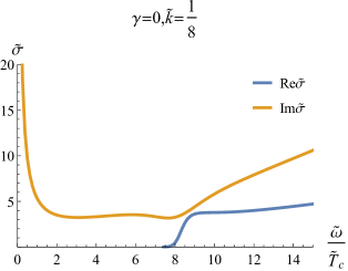
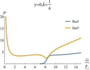
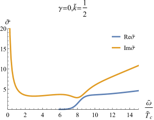
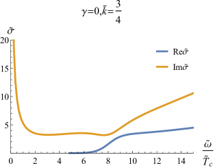
  Figure 7: The frequency behavior of the optical conductivity for various values of $\tilde{k}$, with $\gamma=0$ and $\tilde{T}/\tilde{T_{c}}=0.1$ fixed.

  

  

  

  

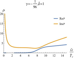
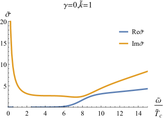
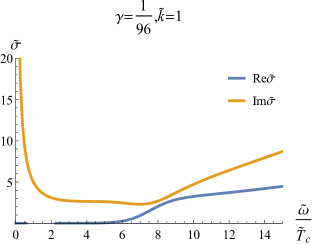
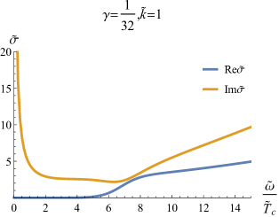
  Figure 8: The frequency behavior of the optical conductivity for various values of $\gamma$, with $\tilde{k}=1$ and $\tilde{T}/\tilde{T_{c}}=0.1$ fixed.

  

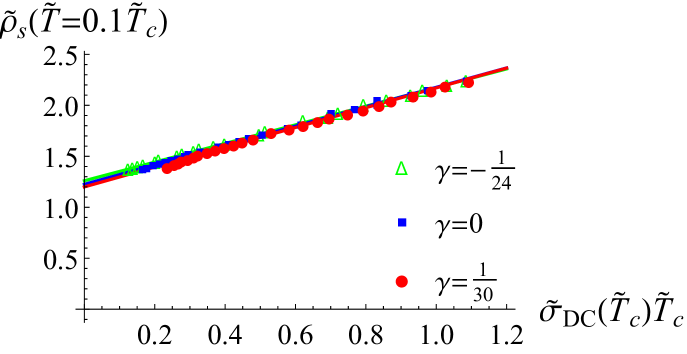
  Figure 9: The plot is for $\tilde{\rho}_{s}(\tilde{T}=0.1\tilde{T_{c}})$ versus $\tilde{\sigma}_{DC}(\tilde{T_{c}})\tilde{T_{c}}$. A linear relation is observed with a fixed $\gamma$ and our fitting gives rise to a modified Home’s law $\tilde{\rho}_{s}=C\tilde{\sigma}_{DC}(\tilde{T_{c}})\tilde{T_{c}}+a$.

  V Discussion

  In this paper we have constructed a holographic model with Weyl corrections in five dimensional spacetime. Momentum relaxation is introduced by the coupling term between the axions and the Maxwell field. For the normal state of the conductivity we find the portion of incoherence is suppressed with the increase of the strength of axions, which is in contrast to the previous holographic models with momentum relaxation induced by axions. For the superconducting phase we have found that the critical temperature decreases with $\tilde{k}$, indicating that the condensation becomes harder in the presence of the axions, while it increases with Weyl parameter. More importantly we find the density of superfluid at zero temperature has a linear relation with the quantity $\tilde{\sigma}_{DC}(\tilde{T_{c}})\tilde{T_{c}}$ which can be described by a modified formula of Homes’ law. Moreover, constant $a\neq 0$ implies superconducting transition would be the first order phase transition at $\tilde{T_{c}}=0$ rather than the second order one and would reflect the property of quantum critical phenomenon.

  Some crucial issues are worth for further investigation. First of all, due to the presence of the Weyl correction, we have only investigated the conductivity of the dual system in the probe limit. It is very interesting to take the backreactions of matter fields to the background into account, which leads to higher order differential equations of motionMyers:2010pk ; Ling:2016dck . In this situation we expect that more abundant phenomena could be observed for the transport behavior of the dual system. In particular, some quantum critical phenomenon such as metal-insulator transition can be implemented and its relation with the holographic entanglement entropy could be investigated as explored in Ling:2016dck . Secondly, we have only considered a special coupling term between the axion fields and Maxwell field, it is quite intriguing to construct more realistic models which could be described by the Homes’ law with a constant compatible with the experimental data. Finally, the incoherent part of the conductivity can approximately be described by a constant $\tilde{\sigma}_{Q}$ only in low frequency region under the condition that the coherent contribution is dominant. It is very worthy of investigating its frequency dependent behavior in a generic situation.

  Acknowledgements

  We are very grateful to Wei-jia Li, Peng Liu, Zhuoyu Xian, Jianpin Wu and Zhenhua Zhou for helpful discussion. We also thank W. Witczak-Krempa for his very valuable comments on the previous version of the manuscript. This work is supported by the Natural Science Foundation of China under Grant Nos.11275208 and 11575195, and by the grant (No. 14DZ2260700) from the Opening Project of Shanghai Key Laboratory of High Temperature Superconductors. Y.L. also acknowledges the support from Jiangxi young scientists (JingGang Star) program and 555 talent project of Jiangxi Province.

  Appendix

  In this appendix we present the detailed derivation from (8) to (9). Without loss of generality, we may start from the perturbation equation (27) with $\gamma=k=0$, then we have

  $$A_{x}^{\prime\prime}(z)+\frac{A_{x}^{\prime}(z)\left(z^{4}g(z)g^{\prime}(z)+z^{3}g(z)^{2}\right)}{z^{4}g(z)^{2}}+\frac{A_{x}(z)\left(\omega^{2}-2g(z)\psi(z)^{2}\right)}{z^{4}g(z)^{2}}=0.$$ (31)

  Since the bulk geometry is asymptotically AdS, the field $A_{x}(z)$ has the following expansion near the boundary $z=0$.

  $$A_{x}(z)=A_{x}^{0}+A_{x}^{2}z^{2}-\frac{1}{2}A_{x}^{0}\omega^{2}z^{2}\log(\Lambda z)+\cdots,$$ (32)

  For convenience, we set $A_{x}^{0}=1$, then obtain

  $$A_{x}(z)=1+A_{x}^{2}z^{2}-\frac{1}{2}\omega^{2}z^{2}\log(\Lambda z)+\cdots,$$ (33)

  Taking the ingoing boundary condition at $z=1$ into account, one usually defines ${A_{x}}(z)=(1-z)^{\frac{-i\omega}{4}}{b_{x}}(z)$. Then inserting it into (31), we have the equation for ${b_{x}}(z)$ as following

  $${b_{x}}^{\prime\prime}(z)+c(z){b_{x}}^{\prime}(z)+d(z){b_{x}}(z)=0,$$ (34)

  where

  $$c(z)=\frac{2(z-1)zg^{\prime}(z)+g(z)(2(z-1)-i\omega z)}{2(z-1)zg(z)}$$ (35)

  and

  $$d(z)= \frac{16\omega^{2}(z-1)^{2}+\omega z^{3}g(z)^{2}(-\omega z+4i)}{16(z-1)^{2}z^{4}g(z)^{2}}$$ (36)

  $$-\frac{4(z-1)g(z)\left(8(z-1)\psi(z)^{2}+i\omega z^{4}g^{\prime}(z)\right)}{16(z-1)^{2}z^{4}g(z)^{2}}.$$

  Correspondingly, we find the asymptotic expansion of ${b_{x}}(z)$ near the boundary to be

  $${b_{x}}(z)=1-\frac{i\omega z}{4}+z^{2}\left(A_{x}^{2}-\frac{\omega^{2}}{32}-\frac{i\omega}{8}\right)-\frac{1}{2}\omega^{2}z^{2}\log(\Lambda z)+\cdots.$$ (37)

  Due to the presence of the logarithmic term which is non-analytical, it is not quite efficient to numerically solve the ODE with Chebyshev polynomials. In particular, it is not quite convenient to extract the coefficients in (33) to calculate the Green’s function for conductivity. Thus, to improve the efficiency in numerics, we find it is convenient to introduce a new variable $a_{x}(z)$ by setting $b_{x}(z)=-\frac{1}{2}\omega^{2}z^{2}\log(\Lambda z)+a_{x}(z)$, then we find the asymptotic behavior of $a_{x}(z)$ is

  $${a_{x}}(z)=1-\frac{i\omega z}{4}+z^{2}\left(A_{x}^{2}-\frac{\omega^{2}}{32}-\frac{i\omega}{8}\right)+\cdots,$$ (38)

  then we get

  $$\frac{2A_{x}^{2}}{A_{x}^{0}}=a_{x}^{\prime\prime}(0)+\frac{\omega^{2}}{16}+\frac{i\omega}{4}.$$ (39)

  Substituting (39) into (8), the formula of conductivity can be expressed in terms of the derivatives of the new variable $a_{x}(z)$ as

  $$\sigma(\omega)=-\frac{i\left(16a_{x}^{\prime\prime}(0)+16\omega^{2}\log\left(\frac{\Lambda}{\nu}\right)-7\omega^{2}+4i\omega\right)}{16\omega}.$$ (40)

  We would like to remark that $a_{x}(0)=1$, otherwise $a_{x}(z)$ would also have nonanalytic terms between the source term and the response term. Similarly, if the expansion of fields have other nonanalytic terms such as $z^{k}$ with non-integer $k$ between source and response, we can get rid of these nonanalytic terms in a parallel way. Finally, this method can be straightforwardly generalized to solve equation group with multiple variables.

References

- (1) S. S. Gubser, Phys. Rev. D 78, 065034 (2008) [arXiv:0801.2977 [hep-th]].
- (2) S. A. Hartnoll, C. P. Herzog and G. T. Horowitz, Phys. Rev. Lett. 101, 031601 (2008) [arXiv:0803.3295 [hep-th]].
- (3) S. A. Hartnoll, C. P. Herzog and G. T. Horowitz, JHEP 0812, 015 (2008) [arXiv:0810.1563 [hep-th]].
- (4) S. A. Hartnoll, Class. Quant. Grav. 26, 224002 (2009) [arXiv:0903.3246 [hep-th]].
- (5) C. P. Herzog, J. Phys. A 42, 343001 (2009) [arXiv:0904.1975 [hep-th]].
- (6) J. McGreevy, Adv. High Energy Phys. 2010, 723105 (2010) [arXiv:0909.0518 [hep-th]].
- (7) G. T. Horowitz, Lect. Notes Phys. 828, 313 (2011) [arXiv:1002.1722 [hep-th]].
- (8) N. Iqbal, H. Liu and M. Mezei, “Lectures on holographic non-Fermi liquids and quantum phase transitions,” arXiv:1110.3814 [hep-th].
- (9) R. G. Cai, L. Li, L. F. Li and R. Q. Yang, Sci. China Phys. Mech. Astron. 58, no. 6, 060401 (2015) [arXiv:1502.00437 [hep-th]].
- (10) A. Ritz and J. Ward, Phys. Rev. D 79, 066003 (2009) [arXiv:0811.4195 [hep-th]].
- (11) R. C. Myers, S. Sachdev and A. Singh, Phys. Rev. D 83, 066017 (2011) [arXiv:1010.0443 [hep-th]].
- (12) S. Sachdev, Ann. Rev. Condensed Matter Phys. 3, 9 (2012) [arXiv:1108.1197 [cond-mat.str-el]].
- (13) W. Witczak-Krempa and S. Sachdev, Phys. Rev. B 86, 235115 (2012) [arXiv:1210.4166 [cond-mat.str-el]].
- (14) J. P. Wu, Y. Cao, X. M. Kuang and W. J. Li, Phys. Lett. B 697, 153 (2011) [arXiv:1010.1929 [hep-th]].
- (15) D. Momeni and M. R. Setare, Mod. Phys. Lett. A 26, 2889 (2011) [arXiv:1106.0431 [physics.gen-ph]].
- (16) W. Witczak-Krempa and S. Sachdev, Phys. Rev. B 87, 155149 (2013) [arXiv:1302.0847 [cond-mat.str-el]].
- (17) W. Witczak-Krempa, E. Sorensen and S. Sachdev, Nature Phys. 10, 361 (2014) [arXiv:1309.2941 [cond-mat.str-el]].
- (18) W. Witczak-Krempa, Phys. Rev. B 89, no. 16, 161114 (2014) [arXiv:1312.3334 [cond-mat.str-el]].
- (19) E. Katz, S. Sachdev, E. S. Sorensen and W. Witczak-Krempa, Phys. Rev. B 90, no. 24, 245109 (2014) [arXiv:1409.3841 [cond-mat.str-el]].
- (20) Y. Ling, P. Liu, J. P. Wu and Z. Zhou, “Holographic Metal-Insulator Transition in Higher Derivative Gravity,” arXiv:1606.07866 [hep-th].
- (21) J. P. Wu, “Momentum dissipation and holographic transport without self-duality,” arXiv:1609.04729 [hep-th].
- (22) G. T. Horowitz, J. E. Santos and D. Tong, JHEP 1207, 168 (2012) [arXiv:1204.0519 [hep-th]].
- (23) G. T. Horowitz, J. E. Santos and D. Tong, JHEP 1211, 102 (2012) [arXiv:1209.1098 [hep-th]].
- (24) G. T. Horowitz and J. E. Santos, JHEP 1306, 087 (2013) [arXiv:1302.6586 [hep-th]].
- (25) Y. Ling, C. Niu, J. P. Wu, Z. Y. Xian and H. b. Zhang, JHEP 1307, 045 (2013) [arXiv:1304.2128 [hep-th]].
- (26) Y. Ling, C. Niu, J. P. Wu and Z. Y. Xian, JHEP 1311, 006 (2013) [arXiv:1309.4580 [hep-th]].
- (27) Y. Ling, C. Niu, J. Wu, Z. Xian and H. b. Zhang, Phys. Rev. Lett. 113, 091602 (2014) [arXiv:1404.0777 [hep-th]].
- (28) A. Donos and S. A. Hartnoll, Nature Phys. 9, 649 (2013) [arXiv:1212.2998].
- (29) A. Donos, B. Goutéraux and E. Kiritsis, JHEP 1409, 038 (2014) [arXiv:1406.6351 [hep-th]].
- (30) A. Donos and J. P. Gauntlett, JHEP 1404, 040 (2014) [arXiv:1311.3292 [hep-th]].
- (31) A. Donos and J. P. Gauntlett, JHEP 1406, 007 (2014) [arXiv:1401.5077 [hep-th]].
- (32) Y. Ling, P. Liu, C. Niu, J. P. Wu and Z. Y. Xian, JHEP 1502, 059 (2015) [arXiv:1410.6761 [hep-th]].
- (33) T. Andrade and B. Withers, JHEP 1405, 101 (2014) [arXiv:1311.5157 [hep-th]].
- (34) B. Goutéraux, JHEP 1404, 181 (2014) [arXiv:1401.5436 [hep-th]].
- (35) K. Y. Kim, K. K. Kim, Y. Seo and S. J. Sin, JHEP 1412, 170 (2014) [arXiv:1409.8346 [hep-th]].
- (36) L. Cheng, X. H. Ge and S. J. Sin, JHEP 1407, 083 (2014) [arXiv:1404.5027 [hep-th]].
- (37) X. H. Ge, Y. Ling, C. Niu and S. J. Sin, Phys. Rev. D 92, no. 10, 106005 (2015) [arXiv:1412.8346 [hep-th]].
- (38) M. Reza Mohammadi Mozaffar, A. Mollabashi and F. Omidi, arXiv:1608.08781 [hep-th].
- (39) C. de Rham, G. Gabadadze and A. J. Tolley, Phys. Rev. Lett. 106, 231101 (2011) [arXiv:1011.1232 [hep-th]].
- (40) S. F. Hassan and R. A. Rosen, Phys. Rev. Lett. 108, 041101 (2012) [arXiv:1106.3344 [hep-th]].
- (41) D. Vegh, “Holography without translational symmetry,” arXiv:1301.0537 [hep-th].
- (42) R. A. Davison, Phys. Rev. D 88, 086003 (2013) [arXiv:1306.5792 [hep-th]].
- (43) M. Blake and D. Tong, Phys. Rev. D 88, no. 10, 106004 (2013) [arXiv:1308.4970 [hep-th]].
- (44) M. Blake, D. Tong and D. Vegh, Phys. Rev. Lett. 112, no. 7, 071602 (2014) [arXiv:1310.3832 [hep-th]].
- (45) Y. Ling, Int. J. Mod. Phys. A 30, no. 28&29, 1545013 (2015).
- (46) S. A. Hartnoll, Nature Phys. 11, 54 (2015) [arXiv:1405.3651 [cond-mat.str-el]].
- (47) R. A. Davison and B. Goutéraux, JHEP 1501, 039 (2015) [arXiv:1411.1062 [hep-th]].
- (48) R. A. Davison and B. Goutéraux, JHEP 1509, 090 (2015) [arXiv:1505.05092 [hep-th]].
- (49) R. A. Davison, B. Goutéraux and S. A. Hartnoll, JHEP 1510, 112 (2015) [arXiv:1507.07137 [hep-th]].
- (50) Z. Zhou, Y. Ling and J. P. Wu, arXiv:1512.01434 [hep-th].
- (51) B. Goutéraux, E. Kiritsis and W. J. Li, JHEP 1604, 122 (2016) [arXiv:1602.01067 [hep-th]].
- (52) C. C. Homes, S. V. Dordevic, M. Strongin, D. A. Bonn, R. Liang, W. N. Hardy, S. Komiya, Y. Ando, G. Yu, N. Kaneko and et al., A universal scaling relation in high-temperature superconductors, Nature 430 (Jul, 2004) 539-541.
- (53) C. C. Homes, S. V. Dordevic, T. Valla and M. Strongin, Scaling of the superfluid density in high-temperature superconductors, Physical Review B 72 (Oct, 2005).
- (54) S. V. Dordevic, D. N. Basov and C. C. Homes, Do Organic and Other Exotic Superconductors Fail Universal Scaling Relations?, Sci. Rep. 3 (Apr, 2013). Article.
- (55) J. Zaanen, Superconductivity: Why the Temperature is High, Nature 430 (Jul, 2004) 512 C513.
- (56) P. Phillips and C. Chamon, Breakdown of One-Parameter Scaling in Quantum Critical Scenarios for High-Temperature Copper-Oxide Superconductors, Physical Review Letters 95 (aug, 2005) 107002 [cond-mat/0412179].
- (57) J. Erdmenger, P. Kerner and S. Muller, JHEP 1210, 021 (2012) [arXiv:1206.5305 [hep-th]].
- (58) J. Erdmenger, B. Herwerth, S. Klug, R. Meyer and K. Schalm, JHEP 1505, 094 (2015) [arXiv:1501.07615 [hep-th]].
- (59) K. Y. Kim, K. K. Kim and M. Park, arXiv:1604.06205 [hep-th].
- (60) K. Y. Kim and C. Niu, “Homes’ law in Holographic Superconductor with Q-lattices,” arXiv:1608.04653 [hep-th].
- (61) T. Andrade and S. A. Gentle, JHEP 1506, 140 (2015) [arXiv:1412.6521 [hep-th]].
- (62) K. Y. Kim, K. K. Kim and M. Park, JHEP 1504, 152 (2015) [arXiv:1501.00446 [hep-th]].
- (63) M. Baggioli and M. Goykhman, JHEP 1507, 035 (2015) [arXiv:1504.05561 [hep-th]].
- (64) M. Baggioli and O. Pujolas, “On holographic disorder-driven metal-insulator transitions,” arXiv:1601.07897 [hep-th].
- (65) M. Taylor, “More on counterterms in the gravitational action and anomalies,” hep-th/0002125.
- (66) R. Gregory, S. Kanno and J. Soda, JHEP 0910, 010 (2009) [arXiv:0907.3203 [hep-th]].
- (67) X. M. Kuang, W. J. Li and Y. Ling, JHEP 1012, 069 (2010) [arXiv:1008.4066 [hep-th]].
- (68) D. Roychowdhury, Phys. Rev. D 86, 106009 (2012) [arXiv:1211.0904 [hep-th]].
- (69) Z. Zhao, Q. Pan and J. Jing, Phys. Lett. B 719, 440 (2013) [arXiv:1212.3062].
- (70) Q. Pan, B. Wang, E. Papantonopoulos, J. Oliveira and A. B. Pavan, Phys. Rev. D 81, 106007 (2010) [arXiv:0912.2475 [hep-th]].
- (71) G. T. Horowitz and M. M. Roberts, JHEP 0911, 015 (2009) [arXiv:0908.3677 [hep-th]].