Anomalous diffusion in time-fluctuating non-stationary diffusivity landscapes

Abstract

We investigate the ensemble and time averaged mean squared displacements for particle diffusion in a simple model for disordered media by assuming that the local diffusivity is both fluctuating in time and has a deterministic average growth or decay in time. In this study we compare computer simulations of the stochastic Langevin equation for this random diffusion process with analytical results. We explore the regimes of normal Brownian motion as well as anomalous diffusion in the sub- and superdiffusive regimes. We also consider effects of the inertial term on the particle motion. The investigation of the resulting diffusion is performed for unconfined and confined motion.

I Introduction

The diffusion of a tracer particle is typically characterised in terms of the mean squared displacement (MSD)

$$\left<x^{2}(t)\right>=\int x^{2}P(x,t)dx=2K_{\gamma}t^{\gamma}$$ (1)

corresponding to the second moment of the probability density function $P(x,t)$ to find the particle at position $x$ at time $t$. When the exponent $\gamma=1$ the law (1) describes normal Brownian diffusion, otherwise we speak of anomalous diffusion. In the latter case, the generalised diffusion coefficient $K_{\gamma}$ has the physical dimensions $\mathrm{cm}^{2}/\mathrm{sec}^{\gamma}$, and we distinguish subdiffusion ($0<\gamma<1$) and superdiffusion ($\gamma>1$) depending on the value of the anomalous diffusion exponent $\gamma$ metz00 .

Following a surge in microscopic techniques, diffusive phenomena of passive tracer particles can now be monitored at unprecedented resolution brauchle . Thus, for instance, the hydrodynamic backflow effects of a Brownian particle could be directly probed jeney . Even more remarkable is the rapidly growing number of experimental evidence for anomalous diffusion in dense fluids dense as well as in living biological cells metz11 ; metz12 ; fran13 ; metz14 ; soko15 ; para15 . The motion of various endogenous and artificial tracers in live cells was shown to be subdiffusive cell ; weis04 ; metz11b . However, when active dynamics such as driving by molecular motors or cytoplasmic streaming are involved, superdiffusion may also be observed cellsuper . Massive computer simulations of pure and protein-crowded lipid bilayer membranes demonstrate transient anomalous diffusion of both lipids and proteins, the crossover to normal diffusion being delayed with increasing disorder lipids ; prx . In the membranes of living cells anomalous diffusion is observed on macroscopic time scales membranes ; lape15 ; metz16 . As a general physical principle for anomalous diffusion various form of crowding of the environment are considered crowd ; ghos15 ; ghos16 . We note that anomalous diffusion also occurs on the level of entire organisms, such as the subdiffusion of bacteria cells in biofilms rogers or the superdiffusion of hydra or protozoa hydra .

Several additional studies of crowded in vitro systems demonstrate the existence of non-Fickian and/or non-Gaussian motion, for instance the glassy dynamics in membrane domains mung16 , confined diffusion of water molecules in soft environments moss16 , polymer diffusion on nanopillar-structured surfaces schw15 , intermittent molecular hopping on solid-liquid interfaces schw13 , colloidal spheres in dense crowded suspensions yeth14 and glasses week00 ; zamp14 , particle diffusion in porous media with heterogeneous and position-dependent mobilities schw15b , and the transport of contaminants in porous and fractured geological formations berk06 . Concurrently the existence of anomalous yet Brownian diffusion—a linear time dependence of the MSD (1) accompanied by significantly non-Gaussian (exponential or stretched exponential) probability density $P(x,t)$—was demonstrated for the motion of colloidal beads along linear phospholipid bilayer tubes gran09 ; gran12 , particle dynamics in hard sphere colloidal suspensions gran14 , and diffusion of nanoparticles in nanopost arrays kris13 .

Brownian motion is bound to the Gaussian shape of the probability density function by the spell of the central limit theorem and thus fully characterised by the second moment (1). In contrast, anomalous diffusion dynamics is inherently non-universal, and therefore a large variety of anomalous diffusion models exists (also with non-Gaussian probability densities), depending on the exact physical circumstances defining the dynamics metz00 ; metz11 ; fran13 ; metz14 ; soko15 ; para15 . To name but a few of these anomalous diffusion processes we recall continuous time random walks with scale free trapping time distributions mont65 and a potential additional noise source noisy , general trapping models traps , correlated diffusion processes corr ; corr1 , fractional Brownian motion fbm and generalised Langevin equation motion fbm ; fle ; pagn16 ; bark09 , as well as diffusion in disordered media and on fractal structures kehr87 ; bray13 ; mard15 .

Here we focus on models based on randomly and/or deterministically varying diffusion coefficients which have recently been under intense study. We show that when the diffusion coefficient varies randomly such that its distribution has a finite width, normal diffusion emerges in the long time limit. We analyse these random diffusion processes (RDPs) in terms of the MSD and time averaged MSD typically evaluated in single particle tracking and simulations studies, for both situations of unconfined and confined diffusion. In addition, we quantify the degree of randomness between different individual trajectories.

In section II we provide a concise overview of heterogeneous diffusion processes, followed by a definition of the various observables for (anomalous) diffusion processes in section III. In section IV we present the details of the specific model investigated here and the numerical scheme used to simulate the RDPs. We then present the main results of our calculations for the ensemble averaged MSD, time averaged MSD, probability distribution function $P(x,t)$, and the ergodic behaviour of RDPs in sections V and VI, respectively, for massless and massive particles. We consider the situation both in the absence and in the presence of an external confinement. Section VII summaries our findings and discusses their possible applications and generalisations.

II Heterogeneous mobility: models and examples

II.1 Random diffusivity models

For massless particles the study of normal and anomalous diffusion in the presence of random diffusivity fields recently attracted considerable attention slat14 ; lape14 ; lape15 ; akim15 ; seba16 . Several models assume that the instantaneous diffusion coefficient $D$ is governed by a steady state distribution $p(D)$ in an annealed fashion, that is, the instantaneous of $D$ is independent of the actual particle position $x$. Particular attention received the idea of a diffusing diffusivity introduced by Chubynsky and Slater slat14 . In their model they assume an exponential distribution

$$p(D)=D_{0}^{-1}\exp[-D/D_{0}]$$ (2)

and weight the standard Gaussian $P(x,D,t)=(4\pi Dt)^{-1/2}\exp(-x^{2}/[4Dt])$ with this function, $\mathfrak{P}(x,t)=\int_{0}^{\infty}p(D)P(x,D,t)dD,$ to obtain the exponential probability distribution function (PDF)

$$\mathfrak{P}(x,t)=\frac{1}{\sqrt{4D_{0}t}}\exp\left[-\frac{|x|}{\sqrt{D_{0}t}}\right].$$ (3)

The characteristic decay length of this PDF grows with the diffusion time as $\simeq t^{1/2}$ slat14 , but the MSD grows linearly with time, that is, follows Eq. (1) with $\gamma=1$ and $K_{\gamma}=D_{0}$ slat14 . Other than exponential diffusivity distributions—for instance, power-law forms of $p(D)$—were shown to lead to subdiffusive and non-ergodic MSD behaviour lape14 . After the current manuscript was submitted, the authors became aware of the simulation-based study egel16 of particle diffusion in rough energy landscapes with both Gaussian and Gamma distributed local energy values.

Dynamical heterogeneities—as reflected in the above assumption of a random diffusivity—are considered a characteristic property of systems such as supercooled or glassy liquids akim15 ; yama98 ; rich02 ; gotz92 ; biro11 . Quite broad distributions of particle diffusivities were detected in a number of living systems, for instance, for the motion of pathogen receptors on two dimensional cell membranes lape15 (see also Ref. saxt97 ), motion of Cajal bodies in eukaryotic nuclei platani , one dimensional diffusion of repressor proteins on the DNA aust06 , and for the motion of proteins along the corrugated landscape created by the DNA sequence goyc14 ; baue15 . In these systems, the inherent stochasticity of the diffusive properties of a tracer particle as well as the heterogeneities of its environment contribute to the observed distribution of diffusivities subsumed in the distribution $p(D)$.

The reader is particularly referred to the characterisation of the dynamical spreading of a population of nematode worms, both in homogeneous and heterogeneous environments hapc09 . Other examples of living systems with diffusing individuals obeying non-Gaussian distribution of diffusivities, speeds of motion $v$, or turning angles are also mentioned in this study. Hapca et al. hapc09 state that the anomalous diffusion monitored in the heterogeneous populations of worms can be solely due to fat-tailed, e.g., gamma distributed yama02 forms of diffusivities, while the motion of each individual remains Brownian. This study served as a strong biological motivation for us in trying to unveil the properties of particle diffusion with a given time dependent form of $p(D,t)$.

Also note that fat-tailed leptokurtic distribution of particle mobilities often occurring in population of individuals of a species can ensure a facilitation of their colonial invasion hapc09 , as compared to the standard Brownian diffusion law of spreading. Such skewed distributions $p(D)$ or $p(v)$ (of the particle speeds) can originate from medium heterogeneities when the organisms explore different regions of space with different mobilities. The notion of fat-tailed distributions and faster than standard front propagation emerges also in long-distance dispersal of plants clar98 ; nath06 and pollen yama04 , in patterns of fish movements skal00 , as well as in rare event driven spreading of plant pathogens hovm02 .

II.2 Deterministic variation of the diffusivity with position or time

Following experimental observations of deterministic gradients of the local diffusivity in both pro- and eukaryotic cells lang11 ; elf11 and the existence of thermal gradient conditions brau13 , the model of heterogeneous diffusion processes (HDPs) with a power-law, exponential, and logarithmic form for $D(x)$ was recently introduced by the authors cher13 ; cher14a ; cher14b ; see also Refs. lenz03 ; fa05 ; zimm11 ; heid14 . These Markovian processes based on a Langevin description with multiplicative noise exhibit anomalous diffusion and weak ergodicity breaking cher13 ; cher14a ; cher14b . The latter emerges due to the fact that even in the limit of long trajectories time and ensemble averages of physical observables do not coincide metz12 ; metz14 , see below. Models with a power-law time dependence

$$D(t)\simeq t^{\alpha-1}$$ (4)

of the diffusivity exist, the so-called scaled Brownian motion (SBM) muni02 ; pein11 ; soko14 ; jeon14 ; safd15 ; grig16 ; metz14 ; bodr15gg . SBM was originally introduced by Batchelor in the description of Richardson turbulence batc52 . Note that in the context of such highly non-stationary processes the degree of ergodicity breaking is controlled via introducing a time- or length-dependent scale into the problem pagn16 ; cher15c . A combined space-time diffusivity dependence of the form $D(x,t)\simeq|x|^{\beta}t^{\alpha-1}$ was also investigated fuli13 ; fuli11 ; cher15b . Aged and confined versions of these processes were recently considered as well cher14b ; jeon15 . Here ageing refers to the explicit dependence of the process on the overall time span of its evolution, as expected for non-stationary processes. The limiting cases with scaling exponent $\beta\to 2$ for HDPs and $\alpha\to 0$ for SBM were shown to lead, respectively, to an ultrafast (exponential) and ultraslow (logarithmic) MSD growth with time cher14c ; lube07 ; bodr15 .

II.3 Massless versus Massive Particles

For massive particles, the situation in anomalous diffusion field is often less clear. While the underdamped limit of standard Brownian motion uhle30 and of fractional Langevin equation motion bark09 are well understood, for other anomalous diffusion processes these limits and general solutions are just emerging. In particular, for SBM it was recently shown that the long time limit of underdamped motion (including the inertia term) does not always correspond to the overdamped limit of the same motion bodr16 . Also, the recent study soko16 addresses a giant particle diffusion in the underdamped limit with a temperature dependent diffusion coefficient and in the presence of a bias. One purpose of the current study is to investigate RDPs for massive and massless particles. A growing interest in the diffusive behaviour of tracked particles combined with the unprecedented precision of experimental observations, in particular, at short times for the diffusion of small particles in living cells rien14 , pose a need for the development of new and more flexible models of stochastic processes. Thus, a larger pool of theoretical models is necessary for quantitative descriptions of these systems, with possibly fewer number of model parameters.

Some implications of a finite particle mass for diffusion processes with position dependent diffusivity of the form $D(x)\simeq|x|^{\beta}$ were recently examined fara17 . The reader is also referred to the studies fara14 ; fara14b regarding the inertial Langevin dynamics in media with space inhomogeneous friction, and conventions of how to interpret the associated multiplicative stochastic equation as well as the existence of fluctuation-dissipation relations for such systems. In what follows, we refer to the diffusion coefficient $D$ as to local variable in space and time, rather as to a long time asymptote of the Einstein relation, see the discussion in Ref. fara14b .

III Observables of diffusion processes

Anomalous diffusion processes can be classified by the MSD diffusion exponent $\gamma$. In single particle tracking and simulations studies garnering few but long individual time series $x(t)$ of the particle position the time averaged MSD metz12 ; metz14

$$\overline{\delta^{2}(\Delta)}=\frac{1}{T-\Delta}\int_{0}^{T-\Delta}\Big{[}x(t+\Delta)-x(t)\Big{]}^{2}dt$$ (5)

is however typically employed. Here $T$ is the total length of the trajectory (observation time) and $\Delta$ is the lag time. Note that while the ensemble averaged MSD (1) is a spatial average at a particular time instant $t$, the time averaged MSD (5) for any given lag time $\Delta$ is taken over the entire history of the trajectory $x(t)$. As usual, ensemble averaging is denoted hereafter by angular brackets, while time averaging is indicated by the overline. To obtain smoother curves for the time averaged MSD an additional average is taken over $N$ trajectories, defining the mean time averaged MSD metz12 ; metz14

$$\left<\overline{\delta^{2}(\Delta)}\right>=\frac{1}{N}\sum_{i=1}^{N}\overline{\delta^{2}_{i}(\Delta)}.$$ (6)

Ergodicity in the Boltzmann-Khinchin sense typically assumed in equilibrium statistical mechanics would imply the equivalence of ensemble and time averaged MSD in the limit of long measurement times, $\lim_{T\to\infty}\overline{\delta^{2}(\Delta)}=\langle x^{2}(\Delta)$. Following Bouchaud bouchaud_web the breakdown of this relation is referred to as weak ergodicity breaking metz08 ; soko08 ; buro10 ; metz11 ; metz14 ; weak ,

$$\lim_{T\to\infty}\overline{\delta^{2}(\Delta)}\neq\left<x^{2}(\Delta)\right>.$$ (7)

Continuous time random walks and HDPs are known to be weakly non-ergodic metz14 , while diffusion on fractals is ergodic on the infinite cluster but not on the entirety of all clusters mard15 . In contrast, other diffusive processes such as fractional Brownian motion and SBM are only marginally non-ergodic jeon10 ; metz14 ; soko14 ; jeon13 ; safd15 ; gode16 ; kurs13 ; greb12 ; jeon14 .

A distinctive measure of non-reproducibility of individual time averaged MSD traces is the ergodicity breaking parameter metz08

$$\mathrm{EB}(\Delta)=\left<\xi^{2}(\Delta)\right>-1$$ (8)

based on the dimensionless ratio $\xi(\Delta)=\overline{\delta^{2}(\Delta)}/\left<\overline{\delta^{2}(\Delta)}\right>$ quantifying the spread of individual time averaged MSDs about their mean (6). Typically EB of a weakly non-ergodic process decays to zero with increasing trace length slower than for the standard Brownian motion bark09 ; greb12 ,

$$\lim_{T\to\infty}\mathrm{EB}_{\mathrm{BM}}(\Delta)=\frac{4\Delta}{3T}.$$ (9)

Or, EB may even attain a finite value as $\Delta/T\to 0$, for instance, for HDPs and continuous times random walks metz08 ; soko08 ; cher13 ; metz14 . Often, also the ratio of the time and ensemble averaged MSDs gode13

$$\mathcal{EB}(\Delta)={\left<\overline{\delta^{2}(\Delta)}\right>}/{\left<x^{2}(\Delta)\right>}$$ (10)

provides additional information about the ergodic properties of the diffusion process.

IV The random diffusivity model

In this section we describe the details of RDPs. As a generalisation of Eq. (2), the instantaneous value of the diffusion coefficient on each simulation step is independently chosen from the Rayleigh distribution

$$p(D)=\frac{D}{D_{\sigma}^{2}}\exp\left[-\frac{D^{2}}{2D_{\sigma}^{2}}\right].$$ (11)

The mean particle diffusivity is then given by

$$\left<D\right>=\sqrt{\pi/2}\times D_{\sigma}$$ (12)

and the diffusivity variance is $\left<(D-\left<D\right>)^{2}\right>=(2-\pi/2)D_{\sigma}^{2}$. Independence of successive values of the diffusion coefficient indicates no temporal correlations in its fluctuations. Our system is thus out of equilibrium (the temperature is not fixed) and the fluctuation dissipation theorem does not hold. The PDF (11) is a smooth function in the range from $D=0$ to $D=\infty$ and it vanishes on the boundaries of this interval. This $p(D)$ distribution is used instead of a Gaussian distributed diffusion coefficient to avoid non-physical negative $D$ values. The distribution (11) is thus physically different from the exponential $p(D)$ form utilised of Chubynsky and Slater in Ref. slat14 . When the mean diffusivity stays constant over time, in the long time limit the particle diffuses normally. However, when the mean diffusivity varies as a power-law,

$$\left<D(t)\right>\simeq t^{\omega},$$ (13)

the resulting process is reminiscent of SBM. Physically, such an increase of the mean diffusivity could be due to a diffusing diffusivity of the form $\langle D(t_{i})\rangle=|\langle D(t_{i-1})\rangle+\zeta_{D}(t_{i-1})|$, where $\zeta_{D}(t_{i})$ is an incremental change. This is analogous to the power-law growth of the waiting times in the correlated continuous time random walk corr1 .

We consider below both massless and massive particles diffusing in both unconfined and a confined environments. We implement the same algorithms for the iterative computation of the particle displacement $x(t)$ as developed for HDPs cher13 and combined HDP-SBM motion cher15b . First, we simulate the one dimensional overdamped Langevin equation

$$\frac{dx(t)}{dt}=\sqrt{2D(t)}\times\zeta(t)$$ (14)

driven by zero-mean and unit-variance Gaussian noise $\zeta(t)$. At step $i+1$ the particle displacement is given by

$$x_{i+1}-x_{i}=\sqrt{2[D(t_{i})+D_{0}]}\times(y_{i+1}-y_{i}),$$ (15)

where $(y_{i+1}-y_{i})$ are the increments of the Wiener process. Unit time intervals separate consecutive steps. To avoid possible particle stalling we regularise $D$ by adding a small constant $D_{0}=10^{-3}$ cher14a ; cher14b . This does not affect the intermediate- and long-time diffusive behaviour. The particle’s initial position is $x_{0}=x(t=0)=0.1.$ In the second part of the paper, we simulate the underdamped Langevin equation for a particle of mass $m$,

$$m\frac{d^{2}x(t)}{dt^{2}}+\eta\frac{dx(t)}{dt}=\sqrt{2D(t)}\times\zeta(t),$$ (16)

with the unit damping coefficient set below to $\eta=1$. At a step $i+1$ the particle displacement is found from the iteration scheme

$$m(x_{i+1}-2x_{i}+x_{i-1})+\eta(x_{i+1}-x_{i})$$

$$=\sqrt{2[D(t_{i})]}\times(y_{i+1}-y_{i}),$$ (17)

where the instantaneous diffusivity is taken from Eq. (11) with the mean (13).

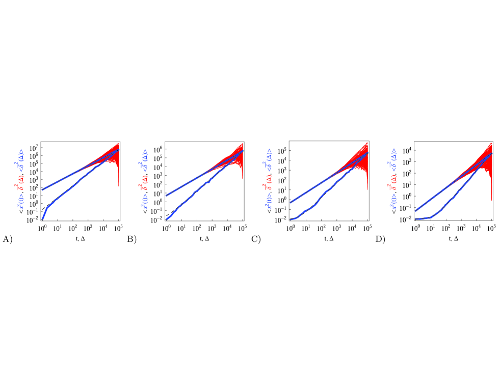
Figure 1: MSD $\left<x^{2}(t)\right>$ and time averaged MSD $\left<\overline{\delta^{2}(\Delta)}\right>$ (thick blue curves) as well as individual time traces $\overline{\delta^{2}(\Delta)}$ (red curves) for overdamped RDPs. The asymptotes (20) and (22) for the MSD and the time averaged MSD are shown by the dashed curves. The asymptotes often superimpose with the results of simulations. Parameters: scaling exponent is $\omega=1/2$, trace length is $T=10^{5}$, and number of traces used for the averaging is $N=150$. The starting position is $x_{0}=0.1$ and the parameter $2\gamma\mathscr{D}/\sqrt{2\pi}$ takes the values $10^{-1}$, $10^{-2}$, $10^{-3}$, and $10^{-4}$ for the panels from left to right. The variable of the $x$ axis is the time $t$ or the lag time $\Delta$.

V Results: Overdamped Motion

V.1 Free Diffusion

We start with the diffusion of massless particles with a fluctuating diffusivity and time invariant mean. As naively expected, we find that due to friction the MSD in the long time limit is Brownian,

$$\left<(x^{2}(t)\right>\sim x_{0}^{2}+2\left<D(t)\right>t.$$ (18)

The MSD and the time averaged MSD are nearly identical after a fast relaxation of the starting position $x_{0}$ of the particle and the ergodicity is approximately fulfilled at all times (results not shown here).

Now we address the more interesting case of RDPs with instantaneous diffusivity chosen from the distribution (11) with a time dependent width (13). Namely, the most likely diffusivity $D_{\sigma}(t)$ at simulation step $i$ is chosen as

$$(D_{\sigma})_{i}=\frac{2\gamma\mathscr{D}}{\sqrt{2\pi}}i^{\omega},$$ (19)

where the prefactor is chosen for convenience and the coefficient $\mathscr{D}$ tunes the magnitude of the diffusivity. From Eq. (14) we straightforwardly compute

$$\left<x^{2}(t)\right>=x_{0}^{2}+2\mathscr{D}t^{\gamma},$$ (20)

with

$$\gamma=1+\omega.$$ (21)

Fig. 1 depicts the case of $\omega=1/2$ or the MSD diffusion exponent $\gamma=3/2$. As can be seen from the simulations the time averaged MSD grows linearly with the lag time $\Delta$, as in the Brownian case. This process also reveals a quite moderate amplitude spread of individual traces $\overline{\delta^{2}(\Delta)}$, see the thin red curves in Fig. 1. Obviously when the lag time approaches the observation time, $\Delta\sim T$, the amplitude scatter increases due to the deteriorating statistic of $\overline{\delta^{2}(\Delta)}$ metz14 . Varying $\mathscr{D}$ in Fig. 1 we demonstrate that, as expected, larger initial diffusivities give rise to a faster approach of the MSD to the theoretical asymptote. In contrast, for rather small diffusivities (smaller $\mathscr{D}$ values) the system needs more time to approach the long time asymptote, Fig. 1. A diminished magnitude of the MSD at smaller $\mathscr{D}$ values inevitably leads to a decrease in the magnitude of the time averaged MSD, see below. At intermediate to long times the superdiffusive MSD regime with $\gamma=3/2$ emerges. Finally, towards the very end of the trace the MSD and the time averaged MSD coincide, as they should metz14 .

Analytically, we obtain for the time averaged MSD from Eq. (14) for $x(t)$ and after averaging over the noise $\zeta(t)$ and diffusion coefficient realisations $p(D)$ the result

$$\left<\overline{\delta^{2}(\Delta)}\right>=\frac{2\mathscr{D}\left[T^{\gamma+1}-(T-\Delta)^{\gamma+1}-\Delta^{\gamma+1}\right]}{(\gamma+1)(T-\Delta)}.$$ (22)

This expression nicely agrees with the results of computer simulations for all $\omega$ and $\mathscr{D}$ values investigated, see Figs. 1 and A1. It is not surprising that both MSD and time averaged MSD are proportional to $\mathscr{D}$ determining the basal value of the particle diffusivity, Eq. (19). In the limit of short lag times, $\Delta\ll T$, from Eq. (22) we recover the scaling behaviour

$$\left<\overline{\delta^{2}(\Delta)}\right>\simeq\frac{2\mathscr{D}\Delta}{T^{1-\gamma}}.$$ (23)

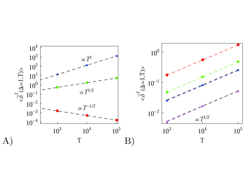
Figure A2: Time averaged MSD versus the trace length $T$ for (A) non-confined overdamped RDPs for $\omega=-1/2,1/2,1$ (for data points from bottom to top) and for (B) non-confined underdamped RDPs for $m=1,5,10,50$ (for data points from top to bottom) and $\omega=1/2$. Other parameters are the same as in Fig. 1 and $2\gamma\mathscr{D}/\sqrt{2\pi}=0.01$. Dashed lines indicate the scaling relation (23) in panel A and Eq. (34) in panel B.

Thus, for superdiffusive RDPs with $\gamma>1$ the magnitude of the time averaged MSD is a growing function of the trace length $T$, while for subdiffusive RDPs $\left<\overline{\delta^{2}}\right>$ magnitude decreases with $T$, in agreement with Fig. A2. In the limit $\Delta\to T$ the ensemble and time averaged MSDs coincide metz14 , as it is easy to check from Eqs. (20) and (22) and corroborated in Fig. 1. The non-equivalence of the time averaged MSD (22) and the time averaged MSD (20) demonstrates that the system is weakly non-ergodic. The scaling behaviour (23) regarding the magnitude of the time averaged MSD in terms of the power law of the trace length $T$ and the linearity in the lag time is analogous to that obtained for subdiffusive continuous time random walks metz10 ; metz11b ; metz08 ; soko08 and their correlated version corr1 as well as for HDPs cher13 ; cher14a ; cher15b and SBM jeon14 ; jeon15 ; see also Ref. metz14 for overview.

For RDPs the ergodicity breaking parameter EB computed from simulations tends to follow the asymptote (9) for Brownian motion at intermediate and long times, Fig. 2. We observe that the initial relaxation of EB to this asymptote is relatively fast. As we show in Fig. 2, after this relaxation time the parameter $\mathcal{EB}$ (10) becomes a power-law function of the lag time $\Delta$,

$$\mathcal{EB}(\Delta)\simeq\Delta^{1-\gamma}.$$ (24)

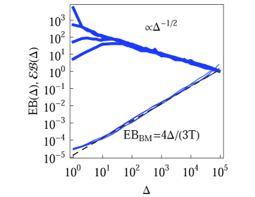
Figure 2: Ergodicity breaking parameter EB and the parameter $\mathcal{EB}$ versus lag time $\Delta$ for overdamped RDPs. The curves are computed for the parameters of Fig. 1 with $\omega=1/2$. The curves for $\mathcal{EB}$ from top to bottom correspond to $2\gamma\mathscr{D}/\sqrt{2\pi}=10^{-1}$, $10^{-2}$, $10^{-3}$, and $10^{-4}$, respectively. The asymptote (9) of Brownian motion and the relation (24) are the dashed lines.

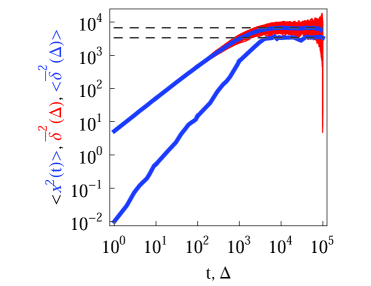
Figure 3: Same as in Fig. 1 but for confined overdamped RDPs. The box size is $L=10^{2}$, $\omega=1/2$, and $2\gamma\mathscr{D}/\sqrt{2\pi}=0.01$. The asymptote (26) and twice this value are the dashed lines.

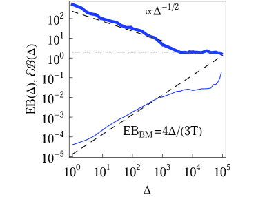
Figure 4: Parameters EB and $\mathcal{EB}$ for confined overdamped RDPs for the parameters of Fig. 3. The Brownian asymptote (9) and the plateau $\mathcal{EB}=2$ are shown as the dashed lines.

Diffusivity distributions $p(D)$ whose mean diffusivity grows with time may be viewed to correspond to an effectively increasing temperature in the system. The opposite case of a temporally shrinking width may stem from a cooling of the system in the course of time. In this respect the current process is reminiscent of SBM jeon14 ; safd15 ; jeon15 . An important example for the latter are granular gases with a relative velocity dependent restitution coefficient bodr15gg .

The particle spreading for very subdiffusive RDPs can be compared to the PDF of SBM, identical to that of fractional Brownian motion for $x_{0}=0$ jeon14 ; muni02 . Namely, after the substitution of the corresponding MSD (20) this produces

$$P(x,t)\sim\frac{1}{\sqrt{4\pi\mathscr{D}t^{\gamma}}}\exp\left(-\frac{x^{2}}{4\mathscr{D}t^{\gamma}}\right).$$ (25)

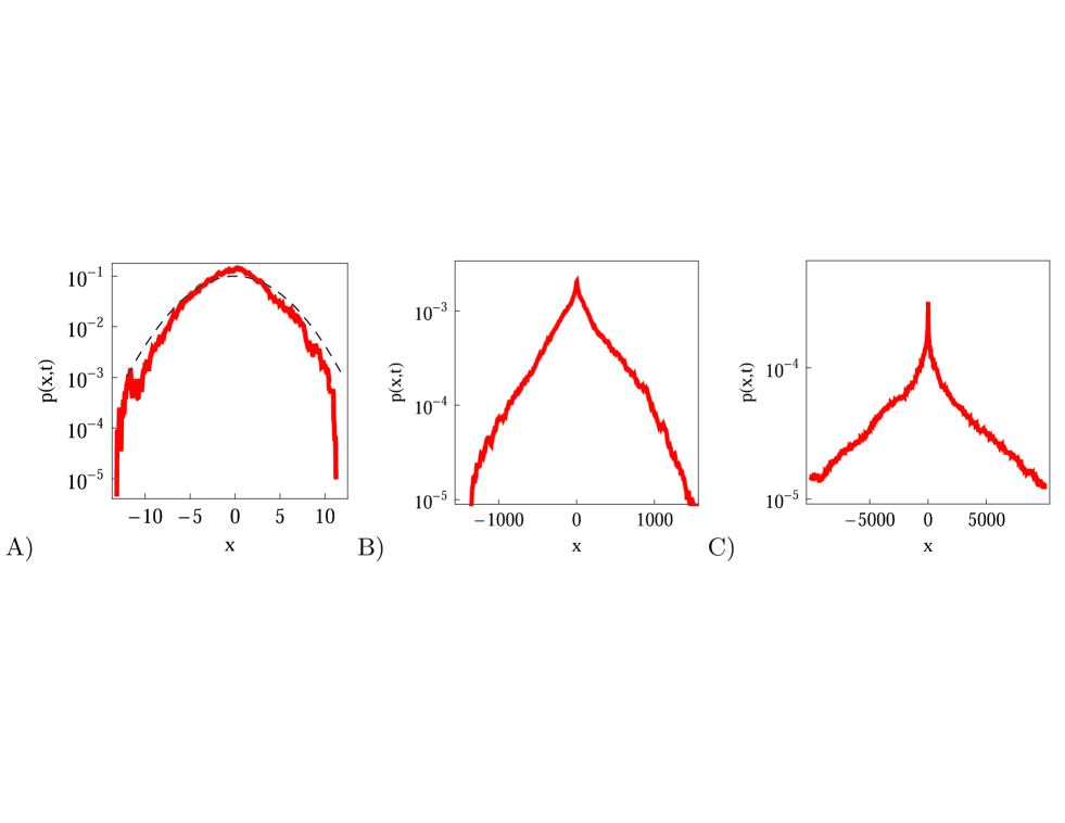
Figure A3: PDF of the overdamped RDPs for $\omega=-1/2$, $1/2$, and $1$ (from left to right). Other parameters are the same as in Fig. 1 with $2\gamma\mathscr{D}/\sqrt{2\pi}=0.01$ and $N=300$. The PDF asymptote for subdiffusive SBM (25) is shown as the dashed curve.

Fig. A3 compares the conjecture (25) with the result from simulations of RDPs. We see, however, that as the MSD scaling exponent increases a distinct cusp of the PDF starts to develop at the origin. The PDF of superdiffusive RDPs becomes pronouncedly non-Gaussian. This spike cannot be described by a convolution of the diffusivity distribution (11) with the kernels of Brownian motion and SBM motion. A more detailed investigation is required to understand this spike at short times and possibly exponential forms of the PDF tails at long times. This generally non-Gaussian and $\alpha$-dependent PDF shape is one important distinction of RDPs with time dependent and in addition fluctuating diffusivities, as compared to the SBM process with the same diffusion coefficient value at each step, $D(t)=\left<D(t)\right>$.

V.2 Confined Diffusion

We now turn to confined RDPs on an interval $-L<x<L$. Such confined motion is important especially for the understanding of diffusion processes in biological cells. In cells, due to their external confinement by the plasma membrane and internal compartmentalisation a diffusing tracer frequently collides with boundaries. As expected, after an initial free diffusion the MSD converges to the stationary plateau metz14

$$\left<x_{\text{st}}^{2}\right>=\frac{1}{2}\left<\overline{\delta^{2}_{\text{st}}}\right>=\frac{1}{3}L^{2},$$ (26)

as demonstrated in Fig. 3. The time averaged MSD, by virtue of its definition (5), approaches twice the value of the MSD in the long time limit. The existence of a plateau is similar to that of standard Brownian motion, and interval-confined SBM and HDPs cher14b ; cher15b . Note that SBM confined by an external potential has a time dependent thermal value of the MSD jeon14 ; jeon15 . The behaviour of confined continuous time random walks is strikingly different, there confinement leads to a crossover to a second power-law regime in the time averaged MSD metz10 ; metz11b . The PDF of confined RDPs approaches a uniform distribution of particles on the interval.

At more severe confinement the ergodicity breaking EB parameter at large lag times $\Delta$ values starts to deviate form the Brownian asymptote (9), see Fig. 4. In addition, we find that for a fixed width of the confining interval and varying trace length $T$ the EB parameter follows the scaling relation

$$\textrm{EB}(T)\simeq 1/T,$$ (27)

as illustrated in Figs. A4A,B. This is a standard decrease of the EB parameter for longer trajectories, a property ubiquitous among a number of both ergodic and non-ergodic stochastic processes metz14 . The decrease of $\mathrm{EB}$ with $T$ indicates a progressively more ergodic diffusion for longer particle traces.

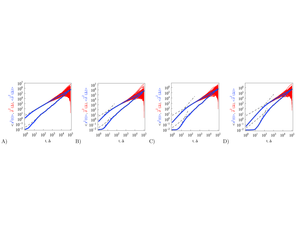
Figure 5: Ensemble averaged MSD, individual time averaged MSDs, and mean time averaged MSD, with the same notation as in Fig. 1, evaluated for underdamped RDPs with particle mass $m=1$, $5$, $10$, and $50$, for panels from left to right. $N\sim 10^{2}$ traces are shown. The long time asymptotes (20) and (22) are the dashed lines. The dot-dashed lines are the asymptotes for the short time regimes, Eqs. (30) and (34). Parameters: $2\gamma\mathscr{D}/\sqrt{2\pi}=0.01$, $\omega=1/2$, and $T=10^{5}$.

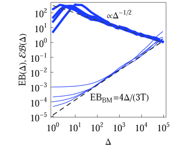
Figure 6: Parameters EB and $\mathcal{EB}$ versus lag time $\Delta$ for underdamped RDPs. The Brownian asymptote (9) and Eq. (24) are the dashed lines. The curves correspond to varying particle mass, $m=1$, $5$, $10$, $50$; the other parameters are the same as in Fig. 5.

VI Results: Underdamped Motion

VI.1 Free Diffusion

In this section, we study the diffusion of massive particles in the same time dependent random diffusivity scenario (19) based on the underdamped Langevin equation. In particular, we explore to what extent inertia effects modify the long time behaviour of the MSD and the time averaged MSD, as compared to the overdamped RDPs considered above. The general solution for the particle MSD follows from the standard procedure for the Brownian motion of massive particles uhle30 . Namely, we obtain

$$x(t)-x(0) = \frac{v_{0}}{\theta}\left(1-e^{-\theta t}\right)$$ (28)

$$-\frac{A}{\theta}e^{-\theta t}\int_{0}^{t}(t^{\prime})^{\omega/2}\zeta(t^{\prime})e^{\theta t^{\prime}}dt^{\prime}$$

$$+\frac{A}{\theta}\int_{0}^{t}(t^{\prime})^{\omega/2}\zeta(t^{\prime})dt^{\prime},$$

where we defined $\theta=\eta/m$ and $A^{2}=2\gamma\mathscr{D}/m^{2}$. Moreover, $v_{0}$ is the initial particle velocity. Then the MSD of the particles after averaging over the noise $\zeta$ can formally be written as

$$\left<x^{2}(t)\right> = x_{0}^{2}+\frac{v_{0}^{2}}{\theta^{2}}\left(1-e^{-\theta t}\right)^{2}$$ (29)

$$-2\gamma\mathscr{D}e^{-2\theta t}\Big{[}t^{\gamma}\mathrm{Ei}(1-\gamma,-2\theta t)\Big{]}_{0}^{t}+2\mathscr{D}t^{\gamma}$$

$$+4\gamma\mathscr{D}e^{-\theta t}\Big{[}t^{\gamma}\mathrm{Ei}(1-\gamma,-\theta t)\Big{]}_{0}^{t}.$$

Here $\mathrm{Ei}(n,z)=\int_{1}^{\infty}e^{-zt}t^{-n}dt$ denotes the generalised exponential integral.

For zero initial velocity of the particles $v_{0}=0$, as in the computer simulations performed here, the inertial term in the Langevin equation gives rise to the initial MSD scaling of the form $\left<x^{2}(t)\right>\sim t^{\gamma+2}$. It is due to progressively accelerating (heating) particles. Explicitly, for the MSD at short times we get

$$\left<x^{2}(t)\right>\sim x_{0}^{2}+\frac{4\mathscr{D}\eta^{2}t^{\gamma+2}}{m^{2}(\gamma+1)(\gamma+2)}.$$ (30)

This faster than ballistic MSD regime often called hyperdiffusion is known to emerge, for instance, for a power-law like transient heating of particles with temperature variation of the form $\mathcal{T}(t)\simeq t^{\omega}$ goyc10 . This superballistic behaviour emerges for RDPs with fluctuating diffusivities and time dependent mean, in analogy with a faster than linear short time ballistic regime in Brownian motion uhle30 .

Note that this short time MSD regime—with the scaling exponent by one larger than the long time exponent—is absent in the model of underdamped scaled Brownian motion elucidated by us recently in Ref. bodr15gg . The reason is that the damping coefficient is set to be temperature independent in the current model, whereas in the model of underdamped SBM the parameter $\eta(t)$ is coupled to law of diffusivity variations via the generalised time-local Einstein relation

$$D(t)=k_{B}T(t)/(m\eta(t))$$ (31)

bodr15gg . So, the fluctuation-dissipation theorem is valid, contrary to the current approach. For the underdamped SBM process, the relation $\eta(t)\sim T^{1/2}(t)$ is consistent with the physical picture of elastically colliding and relaxing particles in a bath with a deterministically varying temperature bodr16 . The reader is also referred to lind07 for studying different relationships between the friction coefficient and velocity for passive and active roma12 particles, including the nonlinear forms.

Note that the diffusive and ergodic properties of underdamped SBM were recently considered too bodr16 . It was demonstrated that the inertial effects relax rather quickly in the course of particle diffusion for $\alpha>1$ situations. This follows from comparing the magnitudes of the acceleration and frictional terms in the Langevin equation. On the other hand, for small positive values of $\alpha$ a finite particle mass yields an extensive intermediate regime, both for the MSD and the time averaged MSD growth behaviour with time. Interestingly, in the case of ultraslow logarithmic SBM motion realised at the boundary value $\alpha=0$ the overdamped limit of particle diffusion bodr15 is not reached at long times, independent on the total measurement time bodr16 .

The time averaged MSD of underdamped RDPs follows from Eqs. (28) and (5),

$$\left<\overline{\delta^{2}(\Delta)}\right> = \frac{A^{2}\eta^{2}}{\theta^{2}(T-\Delta)}\int_{0}^{T-\Delta}dt\left\{\frac{(t+\Delta)^{\gamma}}{\gamma}-\frac{(t)^{\gamma}}{\gamma}\right.$$ (32)

$$-e^{-2\theta(t+\Delta)}\left[t^{\gamma}\mathrm{Ei}(1-\gamma,-2\theta t)\right]_{0}^{t+\Delta}$$

$$-\left(e^{-2\theta t}-2e^{-\theta t}e^{-\theta(t+\Delta)}\right)\left[t^{\gamma}\mathrm{Ei}(1-\gamma,-2\theta t)\right]_{0}^{t}$$

$$+2e^{-\theta(t+\Delta)}\left[t^{\gamma}\mathrm{Ei}(1-\gamma,-\theta t)\right]_{0}^{t+\Delta}$$

$$-\left.2e^{-\theta(t+\Delta)}\left[t^{\gamma}\mathrm{Ei}(1-\gamma,-\theta t)\right]_{0}^{t}\right\}.$$

This integral expression can be evaluated numerically. In the limit of short lag times $\Delta\ll T$ we can evaluate the integral and find

$$\left<\overline{\delta^{2}(\Delta)}\right> \sim \gamma\mathscr{D}\frac{e^{-2\theta T}(-1)^{1-\gamma}}{2(2\theta)^{\gamma-1}}$$ (33)

$$\times\left[\Gamma(\gamma+1)-\Gamma(\gamma+1,-2\theta T)\right]\frac{\Delta^{2}}{T}.$$

Here $\Gamma(a,x)=\int_{x}^{\infty}t^{a-1}e^{-t}dt$ is the generalised incomplete Gamma function and $\Gamma(a,0)=\Gamma(a)$ is the Gamma function. The short time asymptotes of both the MSD and the time averaged MSD are plotted as the dot-dashed curves in Fig. 5 showing nice agreement with the results of computer simulations of Eq. (15).

Expanding the Gamma functions in the corresponding limit we find from expression (33) for light particles or high friction in the system—that is for $\theta T\gg 1$—that

$$\left<\overline{\delta^{2}(\Delta)}\right>\sim\frac{\mathscr{D}\eta T^{\gamma-1}\Delta^{2}}{m}\sim\frac{D(T)\eta\Delta^{2}}{m\gamma}.$$ (34)

This has the form of the short time MSD behaviour of standard Brownian motion uhle30 . All particle masses in this study guarantee the validity of Eq. (34) as the short time expansion for the time averaged MSD in this underdamped limit. Comparing the $\overline{\delta^{2}(T)}$-variation with Eq. (34) in Fig. A2B further supports this validity regarding the dependence on the length of particle trajectory $T$. In the opposite limit of $\theta T\ll 1$—very massive particles or low friction for the particle motion—we find

$$\left<\overline{\delta^{2}(\Delta)}\right>\sim\frac{2\mathscr{D}\eta^{2}T^{\gamma}\Delta^{2}}{m^{2}(\gamma+1)}\sim\frac{\Delta^{2}}{m^{2}}.$$ (35)

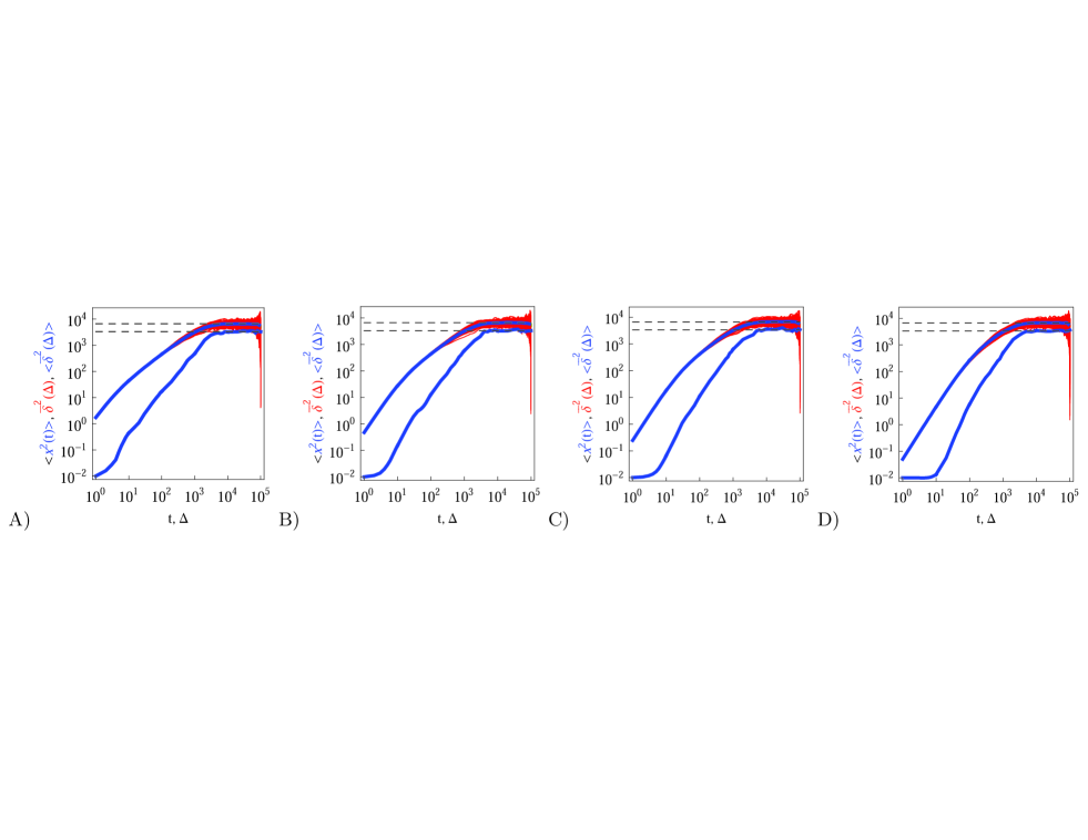
Figure 7: Analogue of Fig. 5 for confined underdamped RDPs with particle mass $m=1$, $5$, $10$, and $50$, from left to right. We show $N=150$ traces for each set of parameters and the interval width is $L=10^{2}$. The asymptotes for the confined motion (26) are the dashed lines.

Let us now describe the results of our computer simulations and compare them with these analytical predictions. We observe that in the particle displacement the initial condition of zero particle velocity ($v_{0}=0$) relaxes within several initial diffusion steps. Naturally, it takes for the system longer to accelerate heavier particles, as shown in Fig. 5 in agreement with Eq. (30). The initial slow acceleration of heavy particles yields slowly growing MSD that gets in turn reflected in small amplitudes of the time averaged MSD at short lag times $\Delta$. The MSD follows Eq. (30) for short times and then crosses over to the long time scaling (20). Note that the same initial quadratic regime was observed in Ref. bodr16 for the short time behaviour of the time averaged MSD of the standard underdamped SBM process. For the time averaged MSD the heavier particles feature a longer ballistic regime, see Fig. 5. The magnitude of $\left<\overline{\delta^{2}}\right>$ decreases with the particle mass, in agreement with Eq. (34). At longer times the MSD and time averaged MSD approach the results expected for the overdamped RDP motion, shown as the long time asymptotes in Fig. 5. As expected, apart from the initial ballistic regime of the time averaged MSD described by Eq. (34), the analytical solution for the overdamped limit (22) describes the long time behavior of the results of our computer simulations.

Similar to the overdamped situation, at short lag times the magnitudes of $\left<\overline{\delta^{2}}\right>$ follow the relation (23), see Fig. A2B. We also observe that for underdamped RDPs the spread of individual $\overline{\delta^{2}}$ traces is similar to that of standard Brownian motion. This small spread is consistent with the observation that the EB parameter for this underdamped RDP motion does not deviate strongly from the Brownian asymptote (9) at intermediate and long times, see Fig. 6. In the region of short $\Delta$ the deviations are quite substantial, particularly for massive particles exhibiting a ballistic initial growth of $\left<\overline{\delta^{2}}\right>$ and a nonlinear growth of the MSD, see Fig. 5. The auxiliary parameter $\mathcal{EB}$—again after the initial particle acceleration—follows the asymptote (24), see the thick curves in Fig. 6. The deviations of EB and $\mathcal{EB}$ at short lag times from the Brownian asymptote is more evident for massive particles.

VI.2 Confined Diffusion

We complete our analysis of RDPs with the study of the underdamped motion in a confining box. We observe that at short time the MSD develops similar to the unconfined scenario. Once the boundary of the confined region is reached, the plateaus start to develop at the same levels as for the overdamped RDP case both for the MSD and time averaged MSD, see Eq. (26) and Fig. 7. Towards the very end of the trajectory at $\Delta=T$, the MSD and the time averaged MSD coincide, as they should metz14 . The longer the entire trajectory, however, the narrower the range of lag times where this convergence takes place, and thus the more precise should be the $\Delta$-sampling in this region that is often computationally costly. This effect was studied in detail for the pure SBM motion confined in harmonic potentials jeon14 and for HDPs confined between the hard walls cher14b ; cher15b .

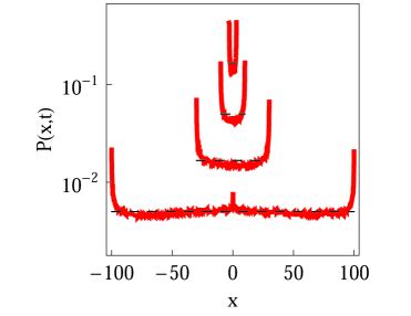
Figure A5: PDF of underdamped confined RDPs for $L=3$, $10$, $30$, and $100$ (from top to bottom), computed for $\omega=1/2$, $2\gamma\mathscr{D}/\sqrt{2\pi}=0.01$, $T=10^{5}$, $m=50$. Dashed lines designate the uniform distribution of particles on the interval.

The PDFs of confined underdamped RDPs at varying box width $L$ is presented in Fig. A5. We observe that for wide intervals the particles are nearly uniformly distributed on the interval (see the dashed lines in Fig. A5), with only insignificant increase in the particle occupancies near the box boundaries due to reflections. Note that the particle starting position at $x=x_{0}$ is still slightly visible in the PDF for a weak confinement. As the confinement becomes more severe, the particle accumulation bear the interval boundaries occupies a larger fraction of space available for diffusion.

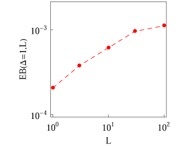
Figure A6: EB parameter at $\Delta=1$ for underdamped RDPs with varying degree of confinement $L$. Parameters are the same as in Fig. A5: $\omega=1/2$, $2\gamma\mathscr{D}/\sqrt{2\pi}=0.01$, $T=10^{5}$, $m=50$.

The EB parameter for massive particles deviates progressively from the Brownian law (9) at both short and long lag times $\Delta$ (not shown). This is due to slow particle acceleration at short times (MSD plateau) and particle confinement at long times, respectively. For free and confined underdamped RDPs—similarly to the overdamped situation—the EB parameter follows the asymptote (27) with the trajectory length $T$, see Figs. A4C,D. As the confinement becomes less severe, the EB parameter approaches the value for the free underdamped RDP motion. Fig. A6 illustrates this EB evolution with the width of the confining interval.

VII Conclusions

We examined the ensemble and time averaged characteristics of random diffusion processes. The randomness of the diffusion coefficient $D$ was implemented in the model via a non-stationary distribution $p(D)$ of diffusivities. RDPs are not thermalised, that is, the motion of the particles is inherently out of equilibrium. The distribution of the diffusion coefficient reflects individual variability of particles diffusivities and heterogeneities of the environment. For typical out-of-equilibrium systems such as biological cells this does not pose any restrictions to our model. RDPs represent a quite flexible model to study asymptotically Brownian and anomalous diffusive systems with a locally fluctuating diffusion coefficient to model physical situations in many complex systems.

We computed both by computer simulations and analytically the MSD, the time averaged MSD, and the ergodicity breaking parameter of RDPs. The unconfined and interval-confined motion were examined. We found that in terms of these standard characteristics subdiffusive RDPs appear similar to subdiffusive SBM with a deterministic diffusivity variation in time. For superdiffusive RDPs the fluctuations grow with time. Concurrently, the average diffusion coefficient $\left<D(t)\right>$ grows with time together with the spread of its values. These features reflect an increasing temperature and more pronounced fluctuations of the medium in the course of particle diffusion. The properties of ageing overdamped and underdamped RDPs will be considered elsewhere.

Living cells feature heterogeneous and densely crowded environments established by a melange of various macromolecules and (importantly) a rather viscoelastic solution between them. This often leads to a broadening in the distribution of diffusion coefficients and subdiffusive exponents, as observed for obstructed diffusion of various tracers saxt97 ; saxt01 ; webb96 ; weis04 . In particular, some extensions of the standard diffusion models to account for these effects—similar to our $p(D)$ distribution for the SBM like diffusion model presented above—appear necessary e.g. for a quantitative fit of fluorescence recovery after photobleaching curves saxt01 . The models of SBM type—with the diffusivity formally decaying in time according to the power law (13)—are often implemented to describe the subdiffusive MSD behavior (1) of the tracer particles in cells. This anomalous MSD scaling was observed e.g. via fitting the shape of the autocorrelation curves of fluorescence correlation spectroscopy measurements webb99 ; weis04 ; weis03 . In single particle tracking measurements in biological cells some time dependent scatter of the diffusion coefficients was also detected saxt97 ; kusu93 . It is necessary in theoretical models i.a. to distinguish between the normal, restricted, and fully trapped populations of the tracers. In fact, a Gamma distribution similar to the Rayleigh distribution (11) used above was proposed in Ref. saxt97 to characterise the scatter of the MSD’s distribution of diffusing particles. On the level of diffusing simple organisms, Gamma like diffusivity distributions were documented for the motion of nematode worms hapc09 . The latter also exhibit non-Gaussian PDFs of the particle displacements with a ”spike” at the origin hapc09 ; hapc07 , similar to some of our findings. Also, the recent study para16 of anomalous and non-ergodic dynamics of particles within a predator-prey model with a broad distribution of diffusion coefficients of interacting partners needs to be mentioned here.

The current study with its preset functional form of the diffusivity distribution and a deterministic law (13) represents a first step into the terrain of stochastic processes with fluctuating and time varying diffusivities. A more general consideration would correspond to a system of coupled stochastic differential equations for the particle position and its diffusivity. The first equation is the standard Langevin equation, while the second equation involves an additional, generally decoupled noise source governing $D(t)$ variation. The correlation function and other noise properties—not necessarily Gaussian—determine then both the ensemble and the time averaged MSDs of diffusing particles cher17 .

Appendix A

In this Appendix we present several additional figures supporting the claims in the main text of the manuscript.

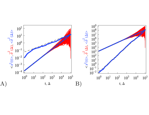
Figure A1: Same as in Fig. 1 but at $\omega=-1/2$ (A) and $\omega=1$ (B) computed for $2\gamma\mathscr{D}/\sqrt{2\pi}=0.01$ and $N=150$. The asymptotes for the MSD and time averaged MSD are shown as the dashed lines.

Figure A4: EB parameter at $\Delta=1$ computed for free and confined overdamped RDPs (panels A, B) and for free and confined underdamped RDPs (panels C, D). Parameters: for all the panels $\omega=1/2$, $2\gamma\mathscr{D}/\sqrt{2\pi}=0.01$ and (panel A: free overdamped process) $m=0$, $L=\infty$; (panel B: confined overdamped process) $m=0$, $L=10^{2}$; (panel C: free underdamped process) $m=50$, $L=\infty$; (panel D: confined underdamped process) $m=50$, $L=10^{2}$.

References

- (1) J.-P. Bouchaud and A. Georges, Phys. Rep. 195, 127 (1990); R. Metzler and J. Klafter, Phys. Rep. 339, 1 (2000); J. Phys. A 37, R161 (2004).
- (2) C. Bräuchle, D. C. Lamb, and J. Michaelis, Single Particle Tracking and Single Molecule Energy Transfer (Wiley-VCH, Weinheim, Germany, 2012); X. S. Xie, P. J. Choi, G.-W. Li, N. K. Lee, and G. Lia, Annu. Rev. Biophys. 37, 417 (2008).
- (3) T. Franosch, M. Grimm, M. Belushkin, F. M. Mor, G. Foffi, L. Forro, and S. Jeney, Nature 478, 7367 (2011).
- (4) D. S. Banks and C. Fradin, Biophys. J. 89, 2960 (2005); G. Guigas, C. Kalla and M. Weiss, Biophys. J. 93, 316 (2007); J. Szymanski and M. Weiss, Phys. Rev. Lett. 103, 038102 (2009); W. Pan, L. Filobelo, N. D. Q. Pham, O. Galkin, V. V. Uzunova, and P. G. Vekilov, Phys. Rev. Lett. 102, 058101 (2009); J.-H. Jeon, N. Leijnse, L. B. Oddershede, and R. Metzler, New J. Phys. 15, 045011 (2013).
- (5) S. Burov, J.-H. Jeon, R. Metzler, and E. Barkai, Phys. Chem. Chem. Phys. 13, 1800 (2011).
- (6) E. Barkai, Y. Garini, and R. Metzler, Phys. Today 65(8), 29 (2012).
- (7) F. Höfling and T. Franosch, Rep. Prog. Phys. 76, 046602 (2013).
- (8) R. Metzler, J.-H. Jeon, A. G. Cherstvy, and E. Barkai, Phys. Chem. Chem. Phys. 16, 24128 (2014).
- (9) Y. Meroz and I. M. Sokolov, Phys. Rep. 573, 1 (2015).
- (10) C. Manzo and M. F. Garcia-Parajo, Rep. Prog. Phys. 78, 124601 (2015).
- (11) A. Caspi, R. Granek, and M. Elbaum, Phys. Rev. E 66, 011916 (2002); G. Seisenberger et al., Science 294, 1929 (2001); I. Golding and E. C. Cox, Phys. Rev. Lett. 96, 098102 (2006); I. Bronstein, Y. Israel, E. Kepten, S. Mai, Y. Shav-Tal, E. Barkai, and Y. Garini, Phys. Rev. Lett. 103, 018102 (2009); S. M. A. Tabei, S. Burov, H. Y. Kim, A. Kuznetsov, T. Huynh, J. Jureller, L. H. Philipson, A. R. Dinner, and N. F. Scherer, Proc. Natl. Acad. Sci. U. S. A. 110, 4911 (2013).
- (12) M. Weiss, M. Elsner, F. Kartberg, and T. Nilsson, Biophys. J. 87, 3518 (2004).
- (13) J.-H. Jeon, V. Tejedor, S. Burov, E. Barkai, C. Selhuber-Unkel, K. Berg-Sorensen, L. Oddershede, and R. Metzler, Phys. Rev. Lett. 106, 048103 (2011).
- (14) A. Caspi, R. Granek, and M. Elbaum, Phys. Rev. Lett. 85, 5655 (2000); N. Gal and D. Weihs, Phys. Rev. E 81, 020903(R) (2010); D. Robert, T. H. Nguyen, F. Gallet, and C. Wilhelm, PLoS ONE 4, e10046 (2010); J. F. Reverey, J.-H. Jeon, H. Bao, M. Leippe, R. Metzler, and C. Selhuber-Unkel, Sci. Rep. 5, 11690 (2015).
- (15) G. R. Kneller, K. Baczynski, and M. Pasienkewicz-Gierula, J. Chem. Phys. 135, 141105 (2011); T. Akimoto, E. Yamamoto, K. Yasuoka, Y. Hirano, and M. Yasui, Phys. Rev. Lett. 107, 178103 (2011); J.-H. Jeon, H. Martinez-Seara Monne, M. Javanainen, and R. Metzler, Phys. Rev. Lett. 109, 188103 (2012); M. Javanainen, H. Hammaren, L. Monticelli, J.-H. Jeon, R. Metzler, and I. Vattulainen, Faraday Discussions 161, 397 (2013); S. Stachura and G. R. Kneller, J. Chem. Phys. 40, 245 (2014); E. Yamamoto, A. C. Kalli, T. Akimoto, K. Yasuoka, and M. S. P. Sansom, Sci. Rep. 5, 18245 (2015).
- (16) J.-H. Jeon, M. Javanainen, H. Martinez-Seara, R. Metzler, and I. Vattulainen, Phys. Rev. X 6, 021006 (2016).
- (17) A. V. Weigel, B. Simon, M. M. Tamkun and D. Krapf, Proc. Natl. Acad. Sci. U. S. A. 108, 6438 (2011); D. Krapf, Curr. Topics Membr. 75, 167 (2015); D. Krapf, G. Campagnola, K. Nepal, and O. B. Peersen, Phys. Chem. Chem. Phys. 18, 12633 (2016).
- (18) R. Metzler, J.-H. Jeon, and A. G. Cherstvy, Biochem. Biophys. (2016). Acta doi:10.1016/j.bbamem.2016.01.022.
- (19) C. Manzo, J. A. Torreno-Pina, P. Massignan, G. J. Lapeyre, Jr., M. Lewenstein, and M. F. Garcia Parajo, Phys. Rev X 5, 011021 (2015).
- (20) H. Berry and H. A. Soula, Front. Physiol. 5, 437 (2014); H. Berry and H. Chate, Phys. Rev. E 89, 022708 (2014); F. Trovato and V. Tozzini, Biophys. J. 107, 2579 (2014); M. Weiss, Intl. Rev. Cell & Molec. Biol. 307, 383 (2014); M. J. Saxton, J. Phys. Chem. B 118, 12805 (2014); D. S. Banks, C. Tressler, R. D. Peters, F. Höfling, and C. Fradin, Soft Matter 12, 4190 (2016); T. Sentjabrskaja, E. Zaccarelli, C. De Michele, F. Sciortino, P. Tartaglia, F. Höfling and T. Franosch, Phys. Rev. Lett. 98, 140601 (2007); S. Leitmann and T. Franosch, Phys. Rev. Lett. 111, 190603 (2013); T. Voigtmann, S. U. Egelhaaf, and M. Laurati, Nature Comm. 7, 11133 (2016).
- (21) S. K. Ghosh, A. G. Cherstvy, and R. Metzler, Phys. Chem. Chem. Phys. 17, 472 (2015).
- (22) S. Ghosh, A. G. Cherstvy, D. S. Grebenkov, and R. Metzler, New. J. Phys. 16, 013027 (2016).
- (23) S. S. Rogers, C. van der Walle, and T. A. Weigh, Langmuir 24, 13549 (2008).
- (24) A. Upadhyaya, J.-P. Rieu, J. A. Glazier, and Y. Sawada, Physica A 293, 549 (2001); L. G. A. Alves, D. B. Scariot, R. R. Guimaraes, C. V. Nakamura, R. S. Mendes, and H. V. Ribeiro, PLoS One 11, e0152092 (2016).
- (25) I. Munguira, I. Casuso, H. Takahashi, F. Rico, A. Miyagi, M. Chami, and S. Scheuring, ACS Nano 10, 2584 (2016).
- (26) S. Hanot, S. Lyonnard, and S. Mossa, Nanoscale 8, 3314 (2016).
- (27) D. Wang, C. He, M. P. Stoykovich, and D. K. Schwartz, ACS Nano 9, 1656 (2015).
- (28) M. J. Skaug, J. Mabry, and D. K. Schwartz, Phys. Rev. Lett. 110, 256101 (2013).
- (29) G. Kwon, B. J. Sung, and A. Yethiraj, J. Phys. Chem. B 118, 8128 (2014).
- (30) E. R. Weeks, J. C. Crocker, A. C. Levitt, A. Schofield, and D. A. Weitz, Science 287, 627 (2000).
- (31) P. Charbonneau, Y. Jin, G. Parisi, and F. Zamponi, Proc. Natl. Acad. Sci. U. S. A. 111, 15025 (2014).
- (32) M. J. Skaug, L. Wang, Y. Ding, and D. K. Schwartz, ACS Nano 9, 2148 (2015); M. J. Skaug and D. K. Schwartz, Ind. Eng. Chem. Res. 54, 4414 (2015).
- (33) B. Berkowitz, A. Cortis, M. Dentz, and H. Scher, Rev. Geophys. 44, RG2003 (2006).
- (34) B. Wang, S. M. Anthony, S. C. Bae, and S. Granick, Proc. Natl. Acad. Sci. U.S.A. 106, 15160 (2009).
- (35) B. Wang, J. Kuo, S. C. Bae, and S. Granick, Nature Mater. 11, 481 (2012).
- (36) J. Guan, B. Wang, and S. Granick, ACS Nano 8, 3331 (2014).
- (37) K. He, F. B. Khorasani, S. T. Retterer, D. K. Thomas, J. C. Conrad, and R. Krishnamoorti, ACS Nano 7, 5122 (2013).
- (38) E. W. Montroll and G. H. Weiss, J. Math. Phys. 6, 167 (1965); H. Scher and E. W. Montroll, Phys. Rev. B 12, 2455 (1975).
- (39) J.-H. Jeon, E. Barkai, and R. Metzler, J. Chem. Phys. 139, 121916 (2013).
- (40) T. Akimoto and E. Barkai, Phys. Rev. E 87, 032915 (2013); T. Akimoto, Phys. Rev. Lett. 108, 164101 (2012); T. Geisel and S. Thomae, Phys. Rev. Lett. 52, 1936 (1984); T. Geisel, J. Nierwetberg and A. Zacherl, Phys. Rev. Lett. 54, 616 (1985); M. W. Deem and D. Chandler, J. Stat. Phys. 76, 911 (1994); C. Monthus and J.-P. Bouchaud, J. Phys. A: Math. Gen. 29, 3847 (1996); E. Bertin and J.-P. Bouchaud, Phys. Rev. E 67, 026128 (2003); S. Burov and E. Barkai, Phys. Rev. Lett. 98, 250601 (2007); M. Dentz et. al., Adv. Water Res. 49, 13 (2012); T. Akimoto, E. Barkai, and K. Saito, arXiv:1604.06175.
- (41) M. M. Meerschaert, E. Nane, and Y. Xiao, Stat. Probab. Lett. 79, 1194 (2009); A. V. Chechkin, M. Hofmann, and I. M. Sokolov, Phys. Rev. E 80, 031112 (2009); J. H. P. Schulz, A. V. Chechkin and R. Metzler, J. Phys. A. 46, 475001 (2013).
- (42) V. Tejedor and R. Metzler, J. Phys. A 43, 082002 (2010); M. Magdziarz, R. Metzler, W. Szczotka, and P. Zebrowski, Phys. Rev. E 85, 051103 (2012);
- (43) B. B. Mandelbrot and J. W. van Ness, SIAM Rev. 10, 422 (1968).
- (44) R. Kubo, Rep. Prog. Phys. 29, 255 (1966); P. Hänggi, Zeit. Physik B 31, 407 (1978); P. Hänggi and F. Mojtabai, Phys. Rev. E 26, 1168 (1982); S. C. Kou, Ann. Appl. Stat. 2, 501 (2008); I. Goychuk, Phys. Rev. E 80, 046125 (2009); I. Goychuk, Adv. Chem. Phys. 150, 187 (2012).
- (45) G. Pagnini, D. Molina-Garcia, T. M. Pham, C. Manzo, and P. Paradisi, E-print arXiv:1508.01361.
- (46) W. Deng and E. Barkai, Phys. Rev. E 79, 011112 (2009).
- (47) J.W. Haus and K. W. Kehr, Phys. Rep. 150, 263 (1987); S. Havlin and D. Ben–Avraham, Adv. Phys. 36, 695 (1987); G. C. Papanicolaou, ”Diffusion in random media”, Surveys in applied mathematics, pp. 205-253 (New York, Plenum Press, 1995); G. M. Zaslavsky, Phys. Rep. 371, 461 (2002); J. P. Bouchaud, A. Comtet, A. Georges, and P. le Doussal, Annal. Phys. 201, 285 (1990).
- (48) A. J. Bray, S. N. Majumdar, G. Schehr, Adv. Phys. 62, 225 (2013).
- (49) Y. Mardoukhi, J.-H. Jeon, and R. Metzler, Phys Chem Chem Phys. 17, 30134 (2015).
- (50) P. Massignan et al., Phys. Rev. Lett. 112, 150603 (2014).
- (51) M. V. Chubynsky and G. W. Slater, Phys. Rev. Lett. 113, 098302 (2014).
- (52) T. Uneyama, T. Miyaguchi, and T. Akimoto, Phys. Rev. E 92, 032140 (2015).
- (53) R. Jain and K. L. Sebastian, J. Phys. Chem. B 120, 3988 (2016).
- (54) J. Bewerunge, I. Ladadwa, F. Platten, C. Zunke, A. Heuer, and S. Egelhaaf, Phys. Chem. Chem. Phys. 18, 18887 (2016).
- (55) W. Gotze and L. Sjogren, Rep. Prog. Phys. 55, 241 (1992).
- (56) R. Yamamoto and A. Onuki, Phys. Rev. Lett. 81, 4915 (1998).
- (57) R. Richert, J. Phys.: Condens. Matter 14, R703 (2002).
- (58) L. Berthier and G. Biroli, Rev. Mod. Phys. 83, 587 (2011).
- (59) M. J. Saxton, Biophys. J. 72, 1744 (1997).
- (60) M. Platani, I. Goldberg, A. I. Lamond, and J. R. Swedlow, Nat. Cell Biol. 4, 502 (2002).
- (61) Y. M. Wang, R. H. Austin, and E. C. Cox, Phys. Rev. Lett. 97, 048302 (2006).
- (62) I. Goychuk and V. O. Kharchenko, Phys. Rev. Lett. 113, 100601 (2014).
- (63) M. Bauer, E. S. Rasmussen, M. A. Lomholt, and R. Metzler, Sci. Rep. 5, 10072 (2015).
- (64) S. Hapca, J. W. Crawford, and L. M. Young, J. R. Soc. Interface 6, 111 (2009).
- (65) K. Yamamura, Popul. Ecol. 44, 93 (2002).
- (66) J. S. Clark, Amer. Naturalist 152, 204 (1998).
- (67) R. Nathan, Science 313, 786 (2006).
- (68) K. Yamamura, Popul. Ecol. 46, 87 (2004);
- (69) G. T. Skalski and J. F. Gilliam, Ecology 81, 1685 (2000).
- (70) J. K. M. Brown and M. S. Hovmoller, Science Translat. Medic. 297, 537 (2002).
- (71) T. Kühn, T. O. Ihalainen, J. Hyvaluoma, N. Dross, S. F. Willman, J. Langowski, M. Vihinen-Ranta, and J. Timonen, PLoS One 6, e22962 (2011).
- (72) B. P. English, V. Hauryliuk, A. Sanamrad, S. Tankov, N. H. Dekker, and J. Elf, Proc. Natl. Acad. Sci. U. S. A. 108, E365 (2011).
- (73) C. B. Mast, S. Schink, U. Gerland, and D. Braun, Proc. Natl. Acad. Sci. U. S. A. 110, 8030 (2013).
- (74) A. G. Cherstvy, A. V. Chechkin, and R. Metzler, New J. Phys. 15, 083039 (2013); A. G. Cherstvy and R. Metzler, Phys. Chem. Chem. Phys. 15, 20220 (2013).
- (75) A. G. Cherstvy, A. V. Chechkin, and R. Metzler, Soft Matter 10, 1591 (2014).
- (76) A. G. Cherstvy, A. V. Chechkin, and R. Metzler, J. Phys. A 47, 485002 (2014).
- (77) K. S. Fa and E. K. Lenzi, Phys. Rev. E 67, 061105 (2003).
- (78) K. S. Fa, Phys. Rev. E 72, 020101(R) (2005).
- (79) M. Burgis et al., New J. Phys. 13, 043031 (2011).
- (80) M. Heidernätsch, PhD Thesis, ”On the diffusion in inhomogeneous systems”, TU Chemnitz (2015).
- (81) H. Safdari, A. G. Cherstvy, A. V. Chechkin, F. Thiel, I. M. Sokolov, and R. Metzler, J. Phys. A 48, 375002 (2015).
- (82) E. Geneston, R. Tuladhar, M. T. Beig, M. Bologna, and P. Grigolini, arXiv:1601.02879.
- (83) S. C. Lim and S. V. Muniandy, Phys. Rev. E 66, 021114 (2002).
- (84) R. Friedrich, J. Peinke, M. Sahimi, and M. R. R. Tabar, Phys. Rep. 506, 87 (2011).
- (85) A. Bodrova, A. V. Chechkin, A. G. Cherstvy, and R. Metzler, Phys. Chem. Chem. Phys. 17, 21791 (2015).
- (86) F. Thiel and I. M. Sokolov, Phys. Rev. E 89, 012115 (2014).
- (87) J.-H. Jeon, A. V. Chechkin, and R. Metzler, Phys. Chem. Chem. Phys. 16, 15811 (2014).
- (88) G. K. Batchelor, Math. Proc. Cambridge Philos. Soc. 48, 345 (1952).
- (89) A. G. Cherstvy and R. Metzler, J. Chem. Phys. 142, 144105 (2015).
- (90) A. Fulinski, J. Chem. Phys. 138, 021101 (2013); Acta Phys. Polon. 44, 1137 (2013).
- (91) A. Fulinski, Phys. Rev. E 83, 061140 (2011).
- (92) A. G. Cherstvy and R. Metzler, J. Stat. Mech. P05010 (2015).
- (93) H. Safdari, A. V. Chechkin, G. R. Jafari, and R. Metzler, Phys. Rev. E 91, 042107 (2015).
- (94) A. G. Cherstvy and R. Metzler, Phys. Rev. E 90, 012134 (2014).
- (95) A. W. C. Lau and T. C. Lubensky, Phys. Rev. E 76, 011123 (2007).
- (96) A. Bodrova, A. V. Chechkin, A. G. Cherstvy, and R. Metzler, New J. Phys. 17, 063038 (2015).
- (97) G. E. Uhlenbeck and L. S. Ornstein, Phys. Rev. 36, 823 (1930).
- (98) A. Bodrova, A. V. Chechkin, A. G. Cherstvy, H. Safdari, I. M. Sokolov, and R. Metzler, Sci. Rep. ???, ??? (2016).
- (99) B. Lindner and I. M. Sokolov, Phys. Rev. E 93, 042106 (2016).
- (100) C. Di Rienzo, V. Piazza, E. Gratton, F. Beltram, and F. Cardarelli, Nature Comm. 5, 5891 (2014).
- (101) S. Regev, N. Gronbech-Jensen, and O. Farago, arXiv:1606.08632.
- (102) O. Farago and N. Gronbech-Jensen, Phys. Rev. E 89, 013301 (2014).
- (103) O. Farago and N. Gronbech-Jensen, J. Stat. Phys. 156, 1093 (2014).
- (104) J.-P. Bouchaud, J. Phys. (Paris) I 2, 1705 (1992).
- (105) G. Bel and E. Barkai, Phys. Rev. Lett. 94, 240602 (2005); A. Rebenshtok, and E. Barkai, Phys. Rev. Lett. 99, 210601 (2007).
- (106) A. Lubelski, I. M. Sokolov, and J. Klafter, Phys. Rev. Lett. 100, 250602 (2008).
- (107) S. Burov, R. Metzler, and E. Barkai, Proc. Natl. Acad. Sci. U. S. A. 107, 13228 (2010).
- (108) Y. He, S. Burov, R. Metzler, and E. Barkai, Phys. Rev. Lett. 101, 058101 (2008).
- (109) J.-H. Jeon and R. Metzler, Phys. Rev. E 81, 021103 (2010).
- (110) J.-H. Jeon, N. Leijnse, L. B. Oddershede, and R. Metzler, New J. Phys. 15, 045011 (2013).
- (111) M. Schwarzl, A. Godec, E. Barkai, and R. Metzler (unpublished).
- (112) A. Andreanov and D. S. Grebenkov, J. Stat. Mech. P07001 (2012).
- (113) J. Kursawe, J. Schulz, and R. Metzler, Phys. Rev. E 88, 062124 (2013).
- (114) A. Godec and R. Metzler, Phys. Rev. Lett. 110, 020603 (2013).
- (115) J.-H. Jeon and R. Metzler, J. Phys. A 43, 252001 (2010).
- (116) P. Siegle, I. Goychuk, and P. Hänggi, Phys. Rev. Lett. 105, 100602 (2010).
- (117) B. Lindner, New J. Phys. 9, 136 (2007); J. Stat. Phys. 130, 523 (2008); New J. Phys. 12, 063026 (2010).
- (118) P. Romanczuk, M. Bär, W. Ebeling, B. Lindner, and L. Schimansky-Geier, Eur. Phys. J. Special Topics 202, 1 (2012).
- (119) M. J. Saxton, Biophys. J. 81, 2226 (2001).
- (120) T. J. Feder, I. Brust-Mascher, J. P. Slattery, B. Baird, and W. W. Webb, Biophys. J. 70, 2767 (1996).
- (121) P. Schwille, J. Korlach, and W. W. Webb, Cytometry 36, 176 (1999).
- (122) M. Weiss, H. Hashimoto, and T. Nilsson, Biophys. J. 84, 4043 (2003).
- (123) A. Kusumi, Y. Sako, and M. Yamamoto, Biophys. J. 65, 2021 (1993).
- (124) S. Hapca, J. W. Crawford, K. MacMillan, M. J. Wilson, and I. M. Young, J. Theor. Biol. 248, 212 (2007).
- (125) C. Charalambous, G. Munoz-Gil, A. Celi, M. F. Garcia-Parajo, M. Lewenstein, C. Manzo, and M. A. Garcıa-March, arXiv:1607.00189.
- (126) A. G. Cherstvy, A. V. Chechkin, and R. Metzler, unpublished.