Chiral magnetism of magnetic adatoms generated by Rashba electrons

Abstract

We investigate long-range chiral magnetic interactions among adatoms mediated by surface states spin-splitted by spin-orbit coupling. Using the Rashba model, the tensor of exchange interactions is extracted wherein a the pseudo-dipolar interaction is found besides the usual isotropic exchange interaction and the Dzyaloshinskii-Moriya interaction. We find that, despite the latter interaction, collinear magnetic states can still be stabilized by the pseudo-dipolar interaction. The inter-adatom distance controls the strength of these terms, which we exploit to design chiral magnetism in Fe nanostructures deposited on Au(111) surface. We demonstrate that these magnetic interactions are related to superpositions of the out-of-plane and in-plane components of the skyrmionic magnetic waves induced by the adatoms in the surrounding electron gas. We show that, even if the inter-atomic distance is large, the size and shape of the nanostructures dramatically impacts on the strength of the magnetic interactions, thereby affecting the magnetic ground state. We also derive an appealing connection between the isotropic exchange interaction and the Dzyaloshinskii-Moriya interaction, which relates the latter to the first order change of the former with respect to the spin-orbit coupling. This implies that the chirality defined by the direction of the Dzyaloshinskii-Moriya vector is driven by the variation of the isotropic exchange interaction due to the spin-orbit interaction.

I Introduction

The lack of inversion symmetry paired with strong spin-orbit (SO) coupling generate the Dzyaloshinskii-Moriya (DM) interaction Dzyaloshinskii (1957); Moriya (1960), a key ingredient for non-collinear magnetism, which is at the heart of chiral magnetism. The DM interaction defines the rotation sense of the magnetization, rotating clockwise or counterclockwise along a given axis of a magnetic material. This is the case of spin-spirals in two-dimensional Bode et al. (2007); Ferriani et al. (2008); Santos et al. (2008) or one-dimensional systems Schweflinghaus et al. (2016); Menzel et al. (2012) down to zero-dimensional non-collinear metallic magnets Khajetoorians et al. (2016); Mankovsky et al. (2009); Antal et al. (2008). This type of interactions is decisive in the formation of the recently discovered magnetic skyrmions (see e.g. Refs. Mühlbauer et al., 2009; Yu et al., 2010; Romming et al., 2013; Heinze et al., 2011), a particular class of chiral spin-texture, which existence was predicted three decades ago Bogdanov and Yablonskii (1989); Roessler et al. (2006). These structures are believed to be interesting candidates for future information technologyBaibich et al. (1988); Crum et al. (2015); Hanneken et al. (2015); Hamamoto et al. (2016) since lower currents are required for their manipulation, in comparison to conventional domain walls Jonietz et al. (2010); Parkin et al. (2008).

The ever-increasing interest in understanding the properties of the DM interaction and the corresponding vector is, thus, not surprising. Although the symmetry aspects of these interactions were discussed in the seminal work of Moriya Moriya (1960), the ingredients affecting the magnitude and the particular orientation of a DM vector are not that explored but are certainly related to the details of the electronic structure. In the context of long-range interactions mediated by conduction electrons, the DM interaction was addressed by SmithSmith (1976) and Fert and LevyFert and Levy (1980). They found a strong analogy with the Ruderman-Kittel-Kasuya-Yosida (RKKY) interactionsRuderman and Kittel (1954); Kasuya (1956); Yosida (1957). Indeed, the long-range DM vector oscillates in magnitude and changes its orientation as function of distance, which was recently confirmed experimentally with scanning tunneling microscopy (STM) and theoretically with ab-initio simulations based on density functional theory Khajetoorians et al. (2016). We note that today, besides theory, state-of-the-art STM experiments can be used to learn about the magnitude, oscillatory behavior and decay of the RKKY interactions as demonstrated in Refs. Zhou et al., 2010; Khajetoorians et al., 2012; Prüser et al., 2014.

Our goal is to address the DM interaction in an analytically tractable model and investigate its magnitude, sign and direction following a bottom-up approach assembling nanostructures of different sizes and shapes, atom-by-atom. We are particularly interested in the long-range magnetic interactions that have been already investigated several times theoretically. For example, Imamura et al.Imamura et al. (2004) considered pairs of localized spins interacting via the so-called two-dimensional Rashba gas of electrons Rashba (1960); Bychkov and I. (1984) while Zhu et al.Zhu et al. (2011) replaced the Rashba gas by the surface of a topological insulator. We revisit the case of Rashba electrons and consider particularly the surface state of Au(111), where the Rashba spin splitting was observed experimentallyLaShell et al. (1996). We report on selected nanostructures: dimers, wires, trimers, and two hexagonal structures deposited on the Au(111), where the interactions are mediated solely by the surface state. For the dimer case, we extract the analytical form of the magnetic exchange interactions tensor using the approximation of Imamura et al.Imamura et al. (2004), labeled in the following RKKY-approximation, without renormalizing the electronic structure of the Rashba electrons because of the presence of the nanostructures. We found an inconsistency in the forms derived in Ref. Imamura et al., 2004, a neglected integrable singularity observed at the minima of the energy dispersion curve, that we correct in the present article. Interestingly, we demonstrate that the magnetic interactions are intimately linked with the magnetization induced by the adatoms forming the dimers. We know, for instance, that a single magnetic adatom generates non-collinear magnetic Friedel oscillations, which can be decomposed into a linear combination of skyrmion-like magnetic waves Lounis et al. (2012). The in-plane components of the induced magnetization define the DM interaction, while the out-of-plane component is related to the usual RKKY-interaction. Also, we go beyond the RKKY-approximation by taking into account the impact of the deposited adatoms, which renormalize the electronic properties and can dramatically modify the long-range magnetic interactions. Moreover, we find an pseudo-dipolar term, or a two-ion anisotropy term generated by the presence of SO coupling, which plays a crucial role in the magnetism of the nanostructures. Although not carefully studied in the literature, these interactions can reach a large magnitude and counter-act the effect of the DM interaction by favoring collinear magnetism. After obtaining all magnetic interactions of interest, we use an extended Heisenberg model to investigate the magnetic states of the selected nanostructures.

II Description of the model

The investigation of the magnetic behavior of the nanostructures is based on an embedding technique, where magnetic impurities are embedded on a surface characterized by the Rashba spin-splitted surface states. Once the electronic structure is obtained, we extract the tensor of magnetic exchange interactions as given in an extended Heisenberg model utilizing a mapping procedure described below.

II.1 Rashba model and embedding technique

The twofold degenerate eigenstates of a two-dimensional electron gas confined in a surface or an interface, i.e. a structure-asymmetric environment, experiences a spin-splitting induced by the spin-orbit interaction. Within the model of Bychkov and RashbaRashba (1960); Bychkov and I. (1984), this splitting effect is grasped by the so-called Rashba Hamiltonian

$$\mathbf{H}=\frac{p^{2}_{x}+p^{2}_{y}}{2m^{*}}~{}{\mathds{1}}_{2}-\frac{\alpha_{\mathrm{so}}}{\hbar}(\boldsymbol{\sigma}_{x}{p_{y}}-\boldsymbol{\sigma}_{y}{p_{x}})\quad,$$ (1)

where ${p_{\gamma}}$, $\gamma\in\{x,y\}$, are the components of the momentum operator $\vec{p}$ in a Cartesian coordinate system with $x,y$ coordinates in the surface plane whose surface normal points along $\hat{e}_{z}$. $m^{*}$ is the effective mass of the electron. $\boldsymbol{\sigma}_{\gamma}$ are the Pauli matrices and $\mathds{1}_{2}$ is the unit matrix in spin-space, with the z-axis of the global spin frame of reference is parallel to $\hat{e}_{z}$. $\alpha_{\mathrm{so}}$ is the Rashba parameter, a measure of the strength of the SO interaction and the parameter that controls the degree of Rashba spin splitting.

The energy dispersion of the Rashba electrons is characterized by the $k$-linear splitting of the free-electron parabolic band dispersion:

$$E_{\mathrm{1(2)}}=\frac{\hbar^{2}}{2m^{*}}(k^{2}_{\mathrm{1(2)}}-k^{2}_{\mathrm{so}})\quad,$$ (2)

with $k_{\mathrm{1(2)}}=\sqrt{k_{\mathrm{so}}^{2}+\frac{2m^{*}E}{\hbar^{2}}}+(-)k_{\mathrm{so}}$ and $k_{\mathrm{so}}=\frac{m^{*}\alpha}{\hbar^{2}}$. For the case of the surface state of the Au(111) surface, $\alpha=-0.4$ eV Å  and $m^{*}=0.26\ m_{\mathrm{e}}$Walls and Heller (2007). We want to calculate the magnetic interactions between magnetic adatoms deposited on a the Rashba electron gas. Therefore, we use an embedding technique, where we connect the Rashba Green function $\boldsymbol{G}^{0}$ to the Green function $\boldsymbol{G}$ of the system Rashba electron gas and magnetic adatoms via a Dyson equation. $\boldsymbol{G}^{0}$, connecting two points separated by $\vec{R}$, is given by:

$$\boldsymbol{G}^{0}(\vec{R},E+i\epsilon)=\left(\begin{array}[]{cc}G_{\text{D}}&-G_{\text{ND}}\,e^{-i\beta}\\ G_{\text{ND}}\,e^{i\beta}&G_{\text{D}}\\ \end{array}\right),$$ (3)

where $G_{D}$ and $G_{ND}$, as defined in the appendix A, depend on the position $\vec{R}$ and energy $E$, while $\beta$ is the angle between $\vec{R}$ and the $x$-axis. When magnetic adatoms are present, the Green function connecting the adatoms sites $i$ and $j$ can be obtained from the Dyson equation:

$$\boldsymbol{G}_{ij}(E)=\boldsymbol{G}_{ij}^{0}(E)+\sum_{km}\boldsymbol{G}_{ik}^{0}(E)\,\boldsymbol{T}_{km}(E)\,\boldsymbol{G}_{mj}^{0}(E)\quad,$$ (4)

Here $\boldsymbol{G}_{ij}^{0}(E)$ is the Rashba Green function connecting sites $i$ and $j$. The full scattering matrix $\boldsymbol{T}(E)$ is given by a Dyson equation:

$$\boldsymbol{{T}}^{-1}_{ij}(E)=\boldsymbol{{t}}_{i}^{-1}(E)\,\delta_{ij}-\boldsymbol{G}^{0}_{ij}(E)\quad,$$ (5)

Where $\boldsymbol{{t}}_{i}(E)$ is the single-site scattering matrix connected to the potential of a single adatom $\boldsymbol{v}_{i}$ via:

$$\boldsymbol{{t}}_{i}(E)=\boldsymbol{{v}}_{i}+\boldsymbol{v}_{i}\,\boldsymbol{G}^{0}_{ii}(E)\,\boldsymbol{{t}}_{i}(E)\quad,$$ (6)

In practice, we proceed to the s-wave approximation Fiete and Heller (2003); Lounis et al. (2012) since the wavelength of Au(111) surface states at the Fermi energy and below are much larger than the size of a single adatom. In this approach, one can work with a single phase shift, $\delta_{j}(E)$, describing the scattering of the surface state at a single impurity: $\mathbf{t}_{j}=\frac{i\hbar^{2}}{m^{*}}\,(e^{2i\delta_{j}(E)}-1)$ at site $j$.

II.2 Extended Heisenberg model

In the extended Heisenberg Hamiltonian $H$ given in , the elements of the magnetic exchange tensor, $\underline{\underline{{\mathbf{J}}}}_{ij}$, can be extracted by differentiating $H$ according to $\vec{e}_{i}$ and $\vec{e}_{j}$:

$$H=\sum_{i,j}\vec{e}_{i}\,\underline{\underline{{\mathbf{J}}}}_{ij}\,\vec{e}_{j}\quad,J_{ij}^{\alpha\beta}=\frac{\partial^{2}{H}}{\partial e_{i}^{\alpha}\partial e_{j}^{\beta}}\quad,$$ (7)

with $\{\alpha,\beta\}=\{x,y,z\}$ and $\vec{e}_{i}$ being the unit vector of the magnetic moment at site $i$. The exchange tensor is decomposed into three contributions:

$$\underline{\underline{{\mathbf{J}}}}_{ij}=\frac{1}{3}\,\mathrm{Tr}\,\{{\underline{\underline{\mathbf{J}}}}_{ij}\}\,{\mathds{1}}_{3}+{\underline{\underline{\mathbf{J}}}}_{ij}^{\text{A}}+\underline{\underline{{\mathbf{J}}}}_{ij}^{\text{S}}\quad.$$ (8)

In the right-hand side of the previous equation, the first term is the isotropic exchange, while $\underline{\underline{{\mathbf{J}}}}_{ij}^{\text{A}}$ is the anti-symmetric part:

$$\underline{\underline{{\mathbf{J}}}}_{ij}^{\text{A}}=\frac{\underline{\underline{{\mathbf{J}}}}_{ij}-\underline{\underline{{\mathbf{J}}}}_{ij}^{\text{T}}}{2}\quad,$$ (9)

it is connected to the Dzyaloshinskii-Moriya vector components via:

$$\underline{\underline{{\mathbf{J}}}}_{ij}^{\text{A}}=\left(\begin{array}[]{rcl}\ 0&\ D_{ij}^{z}&\ -D_{ij}^{y}\\ \--D_{ij}^{z}&\ 0&\ D_{ij}^{x}\\ \ D_{ij}^{y}&\ -D_{ij}^{x}&\ 0\end{array}\right)\quad.$$ (10)

The last term of Eq. 8, $\underline{\underline{{\mathbf{J}}}}_{ij}^{\text{S}}$, is the symmetric part which contains pseudo-dipolar interactions:

$$\underline{\underline{{\mathbf{J}}}}_{ij}^{\text{S}}=\frac{\underline{\underline{{\mathbf{J}}}}_{ij}+\underline{\underline{{\mathbf{J}}}}_{ij}^{\text{T}}}{2}-\frac{1}{3}\,\mathrm{Tr}\,\{{\underline{\underline{\mathbf{J}}}}_{ij}\}\,{\mathds{1}}_{3}\quad.$$ (11)

II.3 Mapping procedure

The strategy is to consider the Hamiltonian describing the electronic structure of the nanostructures and perform the same type of differentiation as in Eq. 7 in order to identify the tensor of magnetic exchange interactions. We use Lloyd’s formula. Lloyd and Smith (1972), which permits the evaluation of the energy variation due to an infinitesimal rotation of the magnetic moments, starting from a collinear configuration Liechtenstein et al. (1987); Udvardi et al. (2003); Ebert and Mankovsky (2009). In general, the contribution to the single-particle energy (band energy) after embedding the nanostructure is given by:

$$E_{sp}=\frac{1}{\pi}\,\mathrm{Im}\int_{E_{R}}^{E_{F}}\mathrm{d}E\,\mathrm{Tr}\,\{\mathrm{ln}\,\boldsymbol{T}(E)^{-1}\}\quad,$$ (12)

where $E_{F}$ is the Fermi energy, $E_{R}=-\frac{\hbar^{2}k^{2}_{\mathrm{so}}}{2m^{*}}$ is the bottom of the Rashba electrons energy dispersion curve and Tr is the trace over impurity position- and spin-indices. The elements of the tensor of exchange interaction are then given by

$$J_{ij}^{\alpha\beta}=\frac{\partial^{2}}{\partial e_{i}^{\alpha}\partial e_{j}^{\beta}}E_{sp}=-\frac{1}{\pi}\,\mathrm{Im}\,\int_{E_{R}}^{E_{F}}\mathrm{d}E\,\mathrm{Tr}\ \{\frac{\,\partial^{2}}{\partial e_{i}^{\alpha}\partial e_{j}^{\beta}}\,\mathrm{ln}\,\boldsymbol{T}(E)\}\quad.$$ (13)

Using Eq. 5, we evaluate the required second derivative and find for the elements of the tensor of exchange interactions:

$$J_{ij}^{\alpha\beta}=-\frac{1}{\pi}\,\mathrm{Im}\,\int_{E_{R}}^{E_{F}}\mathrm{d}E\,\mathrm{Tr}\,\{\mathbf{t}_{i}^{\alpha}\,\mathbf{G}_{ij}\,\mathbf{t}_{j}^{\beta}\,\mathbf{G}_{ji}\}\quad,$$ (14)

the trace is taken over the spin-index, and $\mathbf{t}_{i}^{\alpha}$ is simply the derivative of $\mathbf{t}$ with respect to $e_{i}^{\alpha}$. Since the $\mathbf{t}$-matrix can be written as:

$$\mathbf{t}=\frac{t_{\uparrow}+t_{\downarrow}}{2}\,\mathds{1}_{2}+\frac{t_{\uparrow}-t_{\downarrow}}{2}\,\vec{\boldsymbol{\sigma}}\cdot\vec{e}\quad,$$ (15)

we find that $\mathbf{t}_{i}^{\alpha}=\frac{\partial\mathbf{t}}{\partial e_{i}^{\alpha}}=\Delta_{i}\ {\boldsymbol{\sigma}}^{\alpha}$, with $\Delta=\frac{t_{\uparrow}-t_{\downarrow}}{2}$. The final form of the tensor of magnetic exchange interactions is then finally given by:

$$J_{ij}^{\alpha\beta}=-\frac{1}{\pi}\,\mathrm{Im}\,\int_{E_{R}}^{E_{F}}\mathrm{d}E\,\Delta_{i}\,\Delta_{j}\,\mathrm{Tr}\,\{\boldsymbol{\sigma}^{\alpha}\,\mathbf{G}_{ij}\ \boldsymbol{\sigma}^{\beta}\,\mathbf{G}_{ji}\}\quad.$$ (16)

III Magnetic properties of dimers

III.1 RKKY-approximation

Before the numerical evaluation of the exchange tensor in nanostructures from Eq. 16, it would be interesting to have an approximated analytic form. This is achievable by considering in Eq. 16 the unrenormalized Green functions, $G_{0}$, instead of $G$. Here we recover the RKKY-approximation, expected from second order perturbation theory and used for example by Ref. Imamura et al., 2004. In the particular case of a two-dimensional Rashba electron gas, the Rashba Green function can be expressed using Pauli matrices:

$${\boldsymbol{G}}_{ij}^{0}=G_{D}\,\boldsymbol{\sigma}_{0}-i\,G_{ND}\,(\cos\beta\,\boldsymbol{\sigma}_{y}-\sin\beta\,\boldsymbol{\sigma}_{x})\quad.$$ (17)

Surprisingly, we found anisotropies in the diagonal part of the exchange tensor that are generally neglected in the literature. The physical meaning of these anisotropies can be traced back to the extended Heisenberg model defined by the tensor of magnetic exchange interactions. In fact, by defining the $x$-axis as the line connecting the two sites $i$ and $j$, we show in appendix B that the extended Heisenberg Hamiltonian describing the corresponding magnetic coupling can be written as:

$$\vec{e}_{i}\,\underline{\underline{{\mathbf{J}}}}_{ij}\,\vec{e}_{j}=J\,\vec{e}_{i}\cdot\vec{e}_{j}+D\,(\vec{e}_{i}\times\vec{e}_{j})_{y}+I\,{e}_{i}^{y}\,{e}_{j}^{y}\quad,$$ (18)

where the exchange constants $\{J,D$ and $I\}$ are related to the Rashba Green function by:

$$J=-\frac{2}{\pi}\,\mathrm{Im}\,\int_{E_{R}}^{E_{F}}\mathrm{d}E\,\Delta_{i}\,\Delta_{j}\,(G_{D}^{2}-G_{ND}^{2})\quad,$$ (19)

$$D=\frac{4}{\pi}\,\mathrm{Im}\,\int_{E_{R}}^{E_{F}}\mathrm{d}E\,\Delta_{i}\,\Delta_{j}\,G_{D}\,G_{ND}\quad,$$ (20)

$$I=-\frac{4}{\pi}\,\mathrm{Im}\,\int_{E_{R}}^{E_{F}}\mathrm{d}E\,\Delta_{i}\,\Delta_{j}\,G_{ND}^{2}\quad.$$ (21)

$J$ is the isotropic exchange interaction, which if positive favors an anti-ferromagnetic coupling in our convention, otherwise it favors a ferromagnetic coupling. $D$ is the $y$ component of the D vector, which is by symmetry the only nonzero component (Third rule of Moriya Moriya (1960)). This favors chiral magnetic textures lying in the $xz$ plane. $I$ is the pseudo-dipolar term, a two-ion anisotropy term, coming from the symmetric part of the exchange tensor. It leads to an anisotropy in the diagonal-part of the tensor of exchange interaction, for instance ${J}_{ij}^{xx}={J}_{ij}^{zz}\neq{J}_{ij}^{yy}$. Considering the impurities along the $x$-axis, $I$ is given by ${J}_{ij}^{yy}-{J}_{ij}^{zz}$. This anisotropy is finite because of the two-dimensional nature of the Rashba electrons, so the $x$- and $y$-directions are nonequivalent to the $z$-direction. Here, $I$ favors a collinear magnetic structure along the $y$-axis and counteracts the DM interaction. The analytical forms of the magnetic exchange interactions allow us to understand their origin in terms of the magnetic Friedel oscillations generated by single atoms.Lounis et al. (2012) These oscillations carry a complex magnetic texture that can be interpreted in terms of skyrmionic-like waves. Within the RKKY-approximation and neglecting the energy dependence of $\Delta_{i}$, the isotropic interaction, $J$, connecting two impurities at site $i$ and $j$, is proportional to the $z$-component of magnetization generated at site $j$ by a single impurity at site $i$. In other words, the impurity at site $j$ feels the effective magnetic field generated by the magnetization at that site but induced by the adatom at site $i$. $D$, however, is defined by the in-plane component of the induced magnetization. This is a central result of our work. Here, the corresponding magnetic field felt by the second impurity has an in-plane component and naturally leads to a non-collinear magnetic behavior, i.e. the natural impact of the DM vector. $I$ does not have a simple interpretation, but it can be related to the anisotropy (difference) of the induced magnetization parallel to the impurity moment upon its rotation from out of plane to in plane. In the following we proceed to the analytical evaluation of {$J,D,I$} from the equations above. The details of the integration are given in appendix C.

Evaluation of J. In order to derive analytically the exchange interactions, we use an approximation for the $\mathbf{t}$-matrices. We assume that they are energy independent (Resonant scattering for the minority-spin channel, i.e. $\delta_{\downarrow}=\frac{\pi}{2}$, and no scattering for the majority-spin channel, i.e. $\delta_{\uparrow}={\pi}$), which allows us to write $\Delta_{i}\,=-\frac{2i\hbar^{2}}{m^{*}}$ . This approximation used in Ref. Lounis et al., 2012 is reasonable for an adatom like Fe deposited on Au(111) surface. Then, we find the asymptotic behavior of $G_{D}$ and $G_{ND}$ for large distances $R$ (see appendix C). The isotropic exchange constant can be expressed as:

$$\begin{split}J&=\frac{2}{\pi^{2}R}\,\mathrm{Im}\int_{E_{R}}^{E_{F}}\mathrm{d}E\,\frac{i}{(k_{1}+k_{2})^{2}}\,(k_{1}\,e^{2ik_{1}R}+k_{2}\,e^{2ik_{2}R})\\ &=\frac{\hbar^{2}}{m^{*}\pi^{2}R}\Bigg{[}\,\frac{1}{2R}\sin(2k_{F}R)\cos(2k_{\mathrm{so}}R)-k_{\mathrm{so}}\sin(2k_{\mathrm{so}}R)\ \mathrm{SI}(2k_{F}R)\,\Bigg{]}\quad,\end{split}$$ (22)

where $\mathrm{SI}(x)$ is the sine-integrated function of $x$. $J$ is found to be the sum of two functions. The first one evolves as a function of $\frac{1}{R^{2}}$, as expected for regular two-dimensional systems but the second function decays like $\frac{1}{R}$, which has been neglected in the work of Ref. Imamura et al., 2004. The $\frac{1}{R}$ decay leads to a slower decay of $J$ than what is known for a regular two-dimensional electron gas. It comes from the Van Hove singularity at the bottom of the conduction band at energies below the crossing of the two $k$-splitted bands of the energy dispersion. At very larges distances, $\mathrm{SI}(x)$ converges to a constant ($\frac{\pi}{2}$) and $J$ is behaving like $\frac{1}{R}\sin(2k_{\mathrm{so}}R)$. Naturally, when $k_{\mathrm{so}}$ is set to zero we recover the classical form of the RKKY interaction without spin-orbit coupling for a free electron gas in two-dimensions, i.e. $J$ evolves like $\frac{1}{R^{2}}\sin(2k_{F}R)$.

Evaluation of D. We consider the same approximations used above to calculate the $y$-component of the DM vector ($D$) and find:

$$\begin{split}D&=-\frac{4}{\pi^{2}R}\,\mathrm{Im}\int_{E_{R}}^{E_{F}}\mathrm{d}E\,\frac{1}{2(k_{1}+k_{2})^{2}}\,[\,k_{1}\,e^{2ik_{1}R}-k_{2}\,e^{2ik_{2}R}\,]\quad,\\ &=-\frac{\hbar^{2}}{m^{*}\pi^{2}R}\,\Bigg{[}\,\frac{1}{2R}\sin(2k_{F}R)\sin(2k_{\mathrm{so}}R)+k_{\mathrm{so}}\,\cos(2k_{\mathrm{so}}R)\,\mathrm{SI}(2k_{F}R)\,\Bigg{]}\quad.\end{split}$$ (23)

Like the isotropic exchange constant, $D$ is a sum of two terms. The first term decays as $\frac{1}{R^{2}}$ while the second as $\frac{1}{R}$. A perturbative development of $D$ in terms of $k_{so}$ shows that $D$ is first order in spin-orbit coupling. At very large distances $D$ evolves like $\frac{1}{R}\cos(2k_{\mathrm{so}}R)$.

Evaluation of I. In appendix C, we show that $I$ is a sum of two integrals over the energy because of a branch cut in the Hankel functions. The first integral, denoted $I_{1}$, goes from $E_{R}$ to zero and the second, $I_{2}$, goes from zero to $E_{F}$.

$$\begin{split}I_{1}&=-\frac{4}{\pi^{2}R}\,\mathrm{Im}\int_{E_{R}}^{0}\mathrm{d}E\,\frac{1}{2(k_{1}+k_{2})^{2}}\,\\ &[\,i\,(k_{1}\,e^{2ik_{1}R}+k_{2}\,e^{2ik_{2}R})+2\sqrt{|k_{1}|k_{2}}\,e^{i(k_{2}-|k_{1}|)R}\,\quad,\\ I_{2}&=-\frac{4}{\pi^{2}R}\,\mathrm{Im}\int_{0}^{E_{F}}\mathrm{d}E\,\frac{i}{2(k_{1}+k_{2})^{2}}\\ &[\,k_{1}\,e^{2ik_{1}R}+k_{2}\,e^{2ik_{2}R}\,-2\sqrt{k_{1}k_{2}}\,e^{i(k_{1}+k_{2})R}\,]\quad,\end{split}$$ (24)

and if we sum up the two terms:

$$I=-J+\frac{\hbar^{2}}{m^{*}\pi^{2}R}\Bigg{[}\int_{|k_{\mathrm{so}}|}^{k_{F}}\mathrm{d}q\,\sqrt{1-\frac{k_{\mathrm{so}}^{2}}{q^{2}}}\,\cos(2qR)-\int_{0}^{|k_{\mathrm{so}}|}\mathrm{d}q\,\sqrt{\frac{k_{\mathrm{so}}^{2}}{q^{2}}-1}\,\sin(2qR)\,\Bigg{]}\quad.$$ (25)

The integral involving $\cos(2qR)$ is important at short distances since it competes with one of the terms defining $-J$. In fact, it has the opposite sign of $-\frac{1}{2R}\sin(2k_{F}R)\cos(2k_{\mathrm{so}}R)$ (see Eq. 22). This reduces considerably the value of $I$ comparing to $J$. The second integral involves $\sin(2qR)$ and therefore it leads to a small contribution for low values of $k_{\mathrm{so}}$. A perturbative development of $I$ in terms of $k_{\mathrm{so}}$ shows that $I$ is second order in spin-orbit coupling $(\propto k_{\mathrm{so}}^{2})$.

In Fig. 1(a), we plot the magnetic exchange interactions $J,D$ and $I$ as function of the distance between two magnetic adatoms. The black curve depicts $J$, which at short distances is characterized by a wavelength of $\frac{2\pi}{k_{F}}\sim 37\,$Å. Indeed, from Eq. 22 we expect a beating of the oscillations when $\cos(2k_{\mathrm{so}}R)=0$, in other words at $R=\frac{\pi}{4k_{\mathrm{so}}}\sim 60\,$Å. The latter results from the SO interaction and it is connected to the SO wavelength, $\frac{2\pi}{k_{\mathrm{so}}}\sim 480\,$Å. One notices that for a large range of distances ($R>25$ Å) the magnetic interactions do not oscillate around the $y=0$ axis. This is an artifact of the RKKY-approximation. Similarly to $J$, $D$ is negative for distances larger than $25$ Å, which means within the RKKY-approximation, the chirality defined by the sign of the DM interaction changes only for dimers separated by rather small distances. We notice also that $D$ and $I$ are oscillating functions that can be of the same magnitude as $J$. Thus, we believe that such systems provide the perfect playground to investigate large regions of the magnetic phase diagram inaccessible with usual magnetic materials.

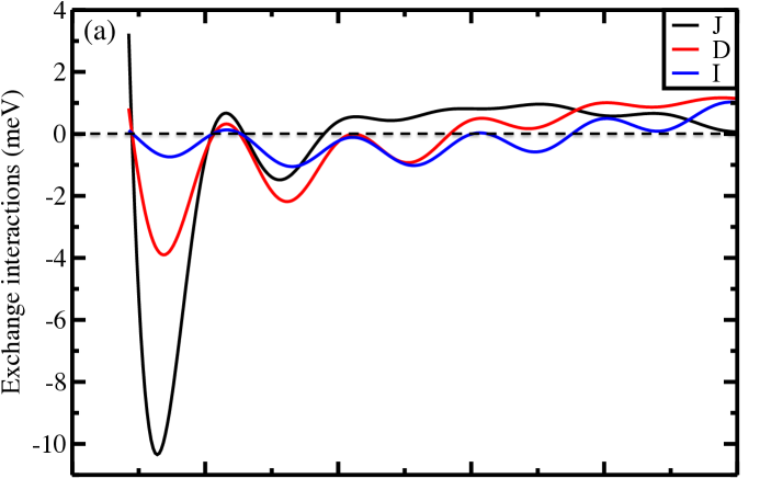
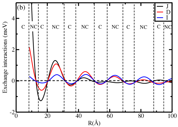
Figure 1: Evolution of the magnetic interactions $J$, $D$, $I$ as a function of the distance by using the RKKY approximation, for $\alpha=-0.4$ eV Å and $m^{*}=0.26\hskip 2.84526ptm_{\mathrm{e}}$ (parameters for Au(111) surface Walls and Heller (2007) used in Eq. 1). (a) We use the RKKY-approximation (see Eqs. 19, 20, 21) and assume a maximal scattering cross section for the minority spin channel ($\delta_{\downarrow}=\frac{\pi}{2}$) and no contribution for the majority spin channel ($\delta_{\uparrow}=\pi$). (b) We go beyond the RKKY-approximation and use the renormalized electronic structure (Eqs. 4 and 16) induced by the presence of two impurities. The vertical lines define a magnetic phase diagram indicating the nature of the orientation of the two magnetic moments as function of their mutual distance. C indicates the collinear phase of the magnetic moments and NC the non-collinear phase.

III.2 Beyond the RKKY-approximation

The deposited magnetic impurities naturally renormalize the electronic properties of the Rashba electrons. To evaluate their impact on the electronic states mediating the magnetic exchange interaction, we numerically compute $\boldsymbol{G}$, by considering consistently the multiple scattering effects. This is done first via considering an energy dependence in the $\mathbf{t}$-matrix assuming that they correspond to a Lorentzian in the electronic structure of the impurities and thus the phase shift is given by $\delta_{\sigma}(E)=\frac{\pi}{2}+\mathrm{atan}\bigg{(}{\frac{E-E_{\sigma}}{\Gamma}}\bigg{)}$. The parameters are extracted from ab-initio Bouaziz et al. (2016), with a band width $\Gamma$ = $0.3\,$eV, and $E_{\downarrow}=0.54\,$eV for the minority-spin channel, slightly on top of the Fermi level $E_{F}=0.41\,$eV, the exchange splitting is $2.8\,$eV with respect to the majority spin-resonance ($E_{\uparrow}=E_{\downarrow}-2.8\,$eV). Then we use (Eq. 5) for computing $\boldsymbol{T}(E)$. Afterwards we solve the Dyson equation (Eq. 4) giving $\boldsymbol{G}$. The evolution of the three exchange interactions after renormalizing the Green function is given in Fig. 1(b). Also we note the disappearance of the RKKY-approximation artifact leading to a non-change of sign of the exchange interaction at very large distances. Indeed, contrary to the curves obtained with the RKKY-approximation, the magnetic interactions oscillate around zero. We traced back this effect to the strong reduction of the quasi one-dimensional behavior of the Rashba electron gas at $E_{R}$ because of the presence of the adatoms. This washes out the sine integrals seen for example in Eqs. 22 and 23.

The beating effect in $J$ occurs at the same distance as in the RKKY-approximation because it is an intrinsic property of the Rashba electron gas. At large distances the intensities of $J$ and $D$ are decreasing quickly, but $I$ keeps oscillating up to a distance of $\sim 200$ Å where it decreases quickly to zero.

III.3 Magnetic configurations of dimers

Having established the behavior of the tensor of magnetic exchange interactions as a function of distance, we investigate now the magnetic ground state of different nanostructures characterized by different geometries and different sizes. After getting the magnetic interactions with the mapping procedure described above, we minimize the extended Heisenberg Hamiltonian with respect to the spherical angles, $(\theta_{i},\phi_{i})$, defining the orientation of every magnetic moment $\vec{e}_{i}=(\cos\phi_{i}\sin\theta_{i},\sin\phi_{i}\sin\theta_{i},\cos\theta_{i})$. In order to check the stability of the magnetic ground state, we often add to the extended Heisenberg Hamiltonian the term $K\sum_{i}{e^{z}_{i}}^{\,2}$, where $K$ is a single-ion magnetic anisotropy energy favoring an out-of-plane orientation of the magnetic moment as it is the case for an Fe adatom on Au(111). We choose as a typical value $K=-6$ meV for all the investigated nanostructures Šipr et al. (2016).

For the particular case of the dimer, an analytical solution is achievable by noticing that two magnetic states are possible: collinear (C) and non-collinear (NC). This is counter-intuitive, since the presence of the DM interaction leads usually to a non-collinear ground state. The presence of the pseudo-dipolar term $I$ makes the physics richer and stabilizes collinear magnetic states. Once more, because of the particular symmetry provided by the Rashba electron gas, within the non-collinear phase, the only finite component of the DM vector, $D_{y}$, enforces the two magnetic moments to lie in $xz$ plane perpendicular to the DM vector. Within the collinear phase, $I$ enforces the moments to point along the $y$-axis.

Non-collinear phase. Here the magnetic moments lie in the $xz$ plane and the pseudo-dipolar term does not contribute to the ground state energy. The ground state is then defined by the angle, $\theta_{0}=\mathrm{atan}\frac{D}{J}$, between the two magnetic moments at sites $i$ and $j$. The energy corresponding to this state is $-|J|\sqrt{1+\frac{D^{2}}{J^{2}}}$. With the single-ion anisotropy, $K$, the ground state angle becomes $\theta_{0}=\hskip 2.84526pt\mathrm{atan}\hskip 2.84526pt(\frac{D}{J+K})$. As an example, we consider two adatoms separated by $d=10.42$ Å which corresponds to the seventh nearest neighbors distance on Au(111). In this case $J=3.45$ meV and $D=0.96$ meV and the ground state angle ($\theta_{0}$) is $164^{\circ}$ $(K=0\,\mathrm{meV})$ or $171^{\circ}$ $(K=-6\,\mathrm{meV})$.

Collinear phase. Here $D$ does not contribute to the ground state configuration. When $J$ and $I$ are both negative the magnetic moments are parallel and point along the axis $y$-axis with the energy $J+I$, while for positive $J$ and $I$ the magnetic moments are anti-parallel and point along the $y$ axis too, with the energy $-(J+I)$. If $J$ and $I$ have opposite signs, for $J>0$ the magnetic moments are anti-parallel in the $(xz)$–plane with the energy $-J$, while for $J<0$ the magnetic moments are parallel in the $(xz)$–plane with the energy $J$. However, these last two solutions will not occur, since the NC phase is lower in energy.

There is competition between the collinear phase C and the non-collinear phase NC, which depends on the involved magnetic interactions. Without $I$, Fig. 1(b) will consist of one single phase, the NC phase. Thanks to $I$, there is an alternation of the two phases depending on the inter-adatom distance. The magnetic anisotropy $K$ favors an out-of-plane orientation of the moments and tends to decrease the spatial range of the collinear phase where the moments point along the $y$-axis.

Phase diagram. In Fig. 2, we plot the phase diagram of the dimers $(K=0\,\mathrm{meV})$. The color scale shows the energy difference ${\Delta E}$ between the ground states found in the NC phase and C phase normalized by $|J|$. A negative (positive) energy difference corresponds to a NC (C) ground state. Thus the blue region corresponds to a C phase and the red region to a NC phase:

$$\begin{cases}&\Delta E=\frac{E_{NC}-E_{C}}{|J|}=-\sqrt{1+\frac{D^{2}}{J^{2}}}+1\quad\text{for}\ J\ \text{and}\ I\ \text{with an opposite sign,}\\ &\Delta E=\frac{E_{NC}-E_{C}}{|J|}=-\sqrt{1+\frac{D^{2}}{J^{2}}}+(1+\frac{I}{J})\quad\text{for}\ J\ \text{and}\ I\ \text{with the same sign.}\\ \end{cases}$$ (26)

For small ratios $\frac{D}{J}$, if $\frac{I}{J}<0$ then $\frac{\Delta E}{|J|}$ simplifies to $-\frac{D^{2}}{2J^{2}}$ and if $\frac{I}{J}>0$ it simplifies to $-\frac{D^{2}}{2J^{2}}+\frac{I}{J}$, which define the magnetic phases plotted in Fig. 2. We notice that when $I$ and $J$ are of the same sign, the dimers are mostly characterized by a C ground state. The corresponding C phase is separated from the NC phase by a parabola as expected from the term $-\frac{D^{2}}{2J^{2}}$. Moreover we note that even within the NC phase, a transition occurs when the sign of $\frac{I}{J}$ changes. This is related to the nature of the NC phase that changes by switching the sign of $\frac{I}{J}$, which leads to an additional, $\frac{I}{J}$, term in the energy difference. As mentioned earlier, if $\frac{I}{J}$ is positive the moments are in plane and align (parallel or anti-parallel) along the $y$ direction, while a negative $\frac{I}{J}$ leads to an alignment in the $(xz)$ plane. For negative $\frac{I}{J}$, one notices that when $\frac{D}{J}$ goes to zero, the plotted energy difference goes to zero, which does not mean that the C and NC phases are degenerate but it is the signature that the rotation angle of the moments goes to zero. Thus at $\frac{D}{J}=0$ we have only a C phase.

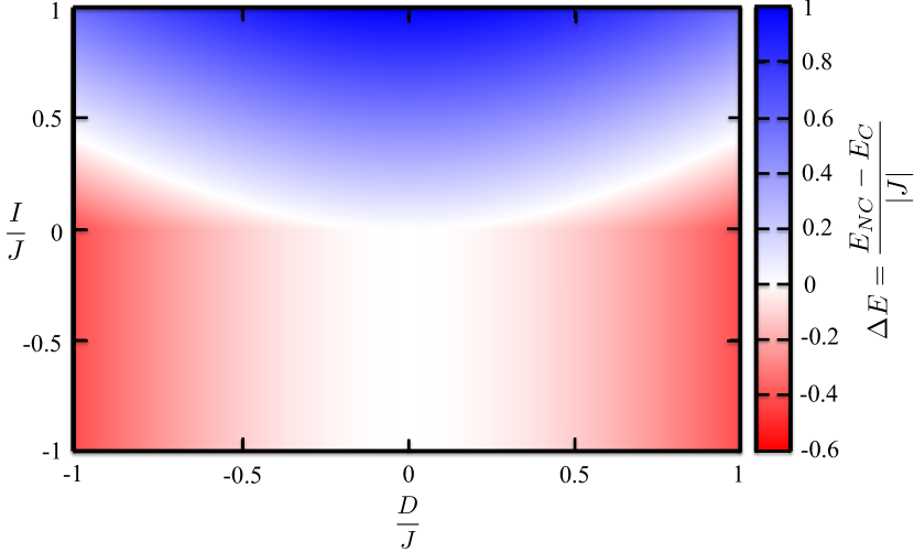
Figure 2: Phase diagram for the magnetic ground states of dimers. The color scale represents the energy difference normalized by $|J|$ between the non-collinear (red color) and collinear states (blue color) as function of the parameters {$\frac{D}{J},\frac{I}{J}$} (see Eq. 26).

Connecting $J$ to $D$. Before investigating nanostructures containing more than two adatoms, it is interesting to analyze the possibility of connecting $J$ to $D$. Recently, it was demonstrated that in the context of a micromagnetic model, the spin stiffness $A\sim\sum_{j}R_{j}^{2}J(R_{j})$, the micromagnetic counterpart of $J$, and $L=\sum_{j}R_{j}D(R_{j})$, the counterpart of $D$ called the Lifshitz invariant can be related to each other for low SO interaction Kim et al. (2013):

$$L\sim-2k_{\mathrm{so}}A\quad.$$ (27)

The sum over sites $j$ is limited by the size of the nanostructure but it can be infinite, e.g. if dealing with a monolayer or an infinite wire.

We checked the validity of the previous relation utilizing the analytical forms of $J$ and $D$ obtained in the RKKY-approximation, i.e. Eqs. 22 and  23, and found that Eq. 27 can be recovered for $k_{so}R<<1$ but the error is proportional to the term involving the sine integral $\mathrm{SI}(2k_{F}R)$. So if one neglects the quasi one-dimensional behavior of the Rashba gas, one gets the formula of Kim et al.Kim et al. (2013).

Instead of the micromagnetic model, we explore in the following the possibility of relating directly $J$ and $D$. We noticed that the derivative of $J$ with respect to $k_{so}$ is proportional to $D$ in the RKKY-approximation:

$$D=\frac{1}{2R}\,\frac{\partial J}{\partial k_{\mathrm{so}}}+\sin(2k_{\mathrm{so}}R)\,\mathrm{SI}(2k_{F}R)\quad.$$ (28)

Once more, if there was no sine integral we would have found a nice way of relating $D$ to $J$. Indeed, the first-order change of $J$ with respect to spin-orbit interaction would lead to the DM interaction $D$:

$$D=\frac{1}{2R}\,\frac{\partial J}{\partial k_{\mathrm{so}}}\quad.$$ (29)

As for the relation of Kim et al. Kim et al. (2013), the error is expected to be large at small distances since $\mathrm{SI}(x)\sim x$. The second term in Eq. 28 cannot be neglected as shown in Fig. 3(a). While the oscillatory behavior of $D$ calculated with Eq. 29 is similar to what is found from Eq. 23, the magnitude of the oscillations and the sign of the interaction is very different. Interestingly, using the renormalized Green functions instead of the RKKY-approximation seems to ameliorate the sine integral issue, similarly to what was found for the magnetic interactions. We recall that in the RKKY-approximation the asymptotic behavior for $J$ and $D$ was peculiar since the sine integral led to a constant shift of the oscillations. This shift was removed when properly renormalizing the Green functions. In the latter case the impact of the quasi one dimensional behavior of the Rashba gas is reduced and the typical van-Hove singularity in the electronic density of states is decreased washing out the contribution of the sine integral. As shown in Fig. 3(b), utilizing Eq. 29 leads then to a more satisfactory description of the exact result.

The intriguing implication of Eq. 29 is that is gives an interpretation for the origin of the chirality being left– or right–handed according to the sign of $D$. For a given distance $R$, $D$ can be of the same (opposite) sign of J if the laters’s magnitude increases (decreases) with the spin-orbit interaction.

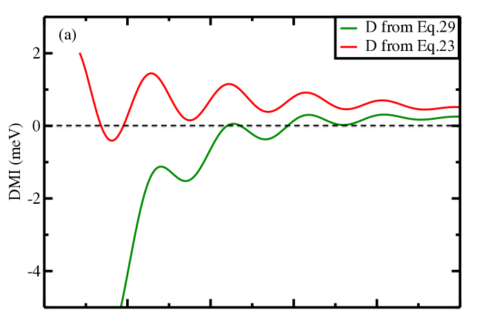
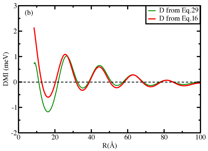
Figure 3: (a) Comparison between $D$ computed from the RKKY-approximation, Eq. 23, and from Eq. 29. (b) The comparison involves $D$ computed from the renormalized Green functions Eq. 16, i.e. beyond the RKKY-approximation, and from Eq. 29.

IV Magnetic properties of other structures

In this section we build magnetic nanostructrures of differents sizes and shapes made of Fe adatoms deposited on Au(111). We compute the magnetic interactions for the considered nanostructrures. A summary of the obtained average magnetic interactions between nearest neighbors is provided in Table. 1.

IV.1 Magnetism of linear chains

Besides dimers, we investigated several linear chains of different sizes. All of them presented the same characteristics. Here we discuss the example of a wire made of 14 adatoms. The distance between the first nearest neighbors is chosen to be $d=10.42$ Å which corresponds to the seventh nearest neighbors distance on Au(111), where the lattice parameter $a=2.87$ Å. This is very close to what is accessible experimentallyKhajetoorians et al. (2012). In this case, the isotropic exchange interaction between the nearest-neighbors is antiferromagnetic. In average it is equal to $6.90$ meV, i.e. the double of the isotropic interaction obtained for the dimer, which highlights the impact of the nanostructure in renormalizing the electronic structure of the system. Within the RKKY-approximation, the magnetic interactions would be independent from the nature, shape, size of the deposited nanostructures. Due to the Moriya rules, the DM vector lies along the $y$-direction within the surface plane similar to the dimer case. It is thus perpendicular to the $x$-axis defined by the chain axis. The DM interaction is around $1.99$ meV between nearest neighbors, i.e. once more the double of the value obtained for the dimer. The magnetic exchange interactions are not limited to the nearest neighbors and follow an oscillatory behavior as function of distance. We compute the ground state starting from differents initial configurations and compute the magnetic states where the torque acting on each magnetic moment is zero, then compare the energy of the obtained magnetic states and select the most stable state. It consists of a spiral contained in the $(xz)$ plane with an average rotation angle of $110^{\circ}$ between two nearest neighboring magnetic moments (see Fig. 4). Interestingly, this angle is much smaller than the one found for the dimer ($164^{\circ}$) but similar to that found for intermediate chains sizes. The pseudo-dipolar term is around $I=0.26$ meV, it has no impact on the ground state since the magnetic moments are contained in the $(xz)$ plane as aformentionned. This situation is equivalent to the $NC$ phase of the dimer, $I$ does not play a role determining the ground state. Of course, choosing an inter-atomic distance with a large pseudo-dipolar term for the dimers, leads generally to stable collinear magnetic wires (not shown here). We noticed that the effect of the magnetic anisotropy energy ($K=-6$ meV ) is mainly on the edge atoms. Indeed, the rotation angles between adjacent inner-moments remain around $110^{\circ}$ while at the edges, the magnetic moments are pointing more along the $z$-direction. The rotation angle between the magnetic moment at the edge and the $z$-axis is reduced to $25^{\circ}$.

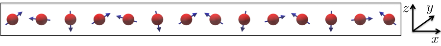
Figure 4: Magnetic ground state of a wire made of 14 adatoms. The spiral is characterized by an average rotation angle of $110^{\circ}$ between nearest neighboring magnetic moments.

IV.2 Magnetism of compact structures

After the one-dimensional case, we address in this section compact structures with the same interatomic distance as the one considered for the wire.

Trimer. We studied a trimer forming an equilateral triangle. The isotropic exchange constant $J$ is equal to $3.51$ meV favoring antiferromagnetic coupling, a value close to the one found for the dimer. The frustration is large in this case leading to a non-collinear ground state even without SO couplingAntal et al. (2008); Lounis (2014). The magnetic moments lie in the same plane, e.g. the surface plane, with an angle of $120^{\circ}$ between two magnetic moments. This state has continuous degeneracy, since rotating each magnetic moment in the same way leaves the energy invariant. If we now consider the DM interaction, we find that $\vec{D}$, with a magnitude of $1.0$ meV (similar to the dimer’s value), lies in the $xy$ plane and perpendicular to the axis connecting two adatoms (see Fig. 5(c)). This interaction lifts the degeneracy present without $D$. As depicted in Fig. 5(a) and (b). The pseudo-dipolar term $I$ is equal to $0.13$ meV and is small compared to $J$ and $D$ therefore the non-collinear phase is more stable. The isotropic interaction keeps the angle between the in-plane projections of the moment at $120^{\circ}$, while the DM interaction generates a slight upward tilting ($81^{\circ}$ instead of $90^{\circ}$). In fact, every DM vector connecting two sites favors the non-collinearity of the related magnetic moments by keeping them in the plane perpendicular to the surface and containing the two sites. This is however impossible to satisfy at the same time for the three pairs of atoms forming the trimer, which leads to the compromise shown in Fig. 5(a) and (b). The magnetic anisotropy reduces ($K=-6$ meV) considerably the non-collinearity and the three moments are enforced to point almost-parallel to the $z$-axis. Two of the magnetic moments are characterized by an angle of $10^{\circ}$ instead of $81^{\circ}$ with respect to the $z$-axis, while the angle of the third moment is $173^{\circ}$ as shown in Fig. 5(d). This is an interesting outcome compared to the behavior of the wire, which is characterized by a large averaged DM interaction in comparison to the trimer. Obviously the shape of the nanostructure is important in stabilizing non-collinear magnetism.

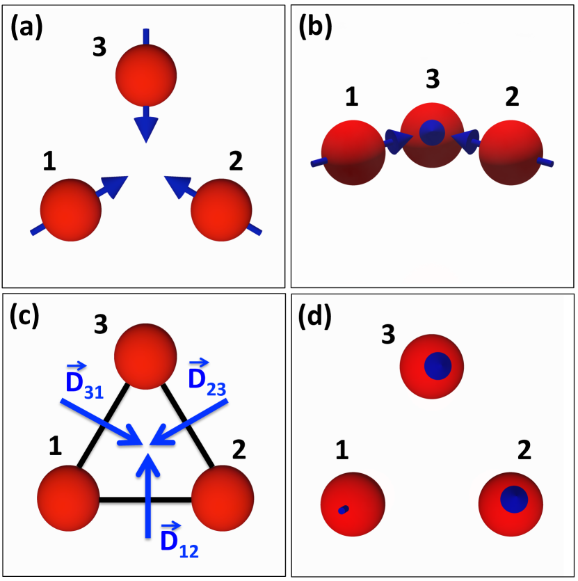
Figure 5: Top view (a) and side view (b) of the non-collinear magnetic configuration for a trimer with an equilateral triangle ($K=0$ meV). While the antiferromagnetic $J$ leads to the $120^{\circ}$ configuration, the DM interaction induces a slight upward tilting of the magnetic moments. The corresponding DM vectors are plotted in (c). (d) Top view for the magnetic ground state of the trimer with $K=-6$ meV.

Structures	J (meV)	D (meV)	I (meV)	$\theta$(∘)
Chain	6.90	1.99	0.26	110
Trimer	3.51	1.00	0.13	117
Hexagone	5.64	1.67	0.23	164
Heptamer	4.69 (4.62)	1.37 (1.36)	0.18 (0.12)	120 (142)

Table 1: Summary of the average magnetic interactions between nearest neighbors for the calculated magnetic nanostructures. The values between parenthesis for the heptamer are for the nearest neighbors on the outer ring.

Hexagonal. We consider now a system of six atoms forming a hexagonal shape with the same interatomic distance as the one considered earlier. The magnetic ground state configuration is non-collinear as shown in Figs. 6(a) and (b). The isotropic magnetic exchange interaction, $J$, between nearest neighbors is of antiferromagnetic type similarly to the value obtained for the other nanostructures studied so far. $J$ reaches a value of 5.64 meV, which is rather close to the interaction found for the wire. In fact one could consider this hexagonal structure as a closed wire. The magnitude of the DM vector connecting two nearest neighbors is large, $1.67$ meV, but not as large as the one of the wire. The non-collinear state is better appreciated when plotting the projection of the moments unit vectors on the surface plane in Fig. 6(c) and along the $z$-axis in Fig. 6(d). The sequence of the polar angles for every pair of nearest neighboring magnetic moments is given by $(16^{\circ},164^{\circ})$ and the azimuthal angle follows the symmetry of the hexagon, leading to an angle difference of $120^{\circ}$ between adjacent moments. The magnetic texture is a compromise involving the antiferromagnetic $J$ and the DM vectors (plotted in Fig.6(e)). While $J$ tries to make the moments anti-parallel to each other, the DM vector tends to make them lie in the plane perpendicular to the surface and containing at the same time the two pairs of atoms (similar to the dimer configuration). However, the magnetic moment has to satisfy the DM vectors arising from its nearest neighbors and therefore, the moment compromises and lies in the plane perpendicular to the surface and containing the atom of interest and the center of the hexagon. This is similar to what was found for the compact trimer. To test the stability of the non-collinear structure, we add the magnetic anisotropy energy and the sequence of polar angles changes from $(16^{\circ},164^{\circ})$ to $(9^{\circ},171^{\circ})$, i.e. a change of $\approx 5^{\circ}$, which is not that large. The interaction with the second and third nearest neighbors are respectively $0.40$ meV and $0.16$ meV, which are small compared to the first nearest neighbors. Thus, they will not affect the ground state considerably.

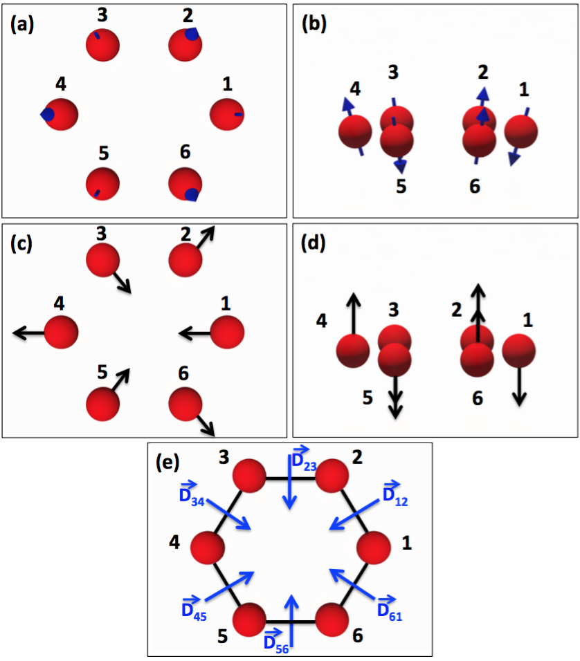
Figure 6: Top (a) and side (b) view of the magnetic ground state configuration for a hexagon made of six atoms. The projection of the unit vectors of the magnetic moments on the surface plane is given in (c) and the projection along the $z$-axis in (d). The corresponding DM vectors between the nearest neighbors are plotted in (e).

Heptamer. We add to the previous structure an atom in the center of the hexagon. Contrary to the other atoms this central atom has six neighbors and the magnetic ground state is profoundly affected by this addition as shown in Fig. 7(a-b). The nearest neighbor isotropic exchange constant $J$, 4.69 meV, decreases slightly in comparison to the value found for the open structure. The obtained magnetic texture can be explained from the nearest neighboring DM interaction (1.37 meV) with the corresponding vectors plotted in Fig. 7(e). The addition of the central atom creates frustration similar to the trimer case. Ideally, every pair of nearest neighboring moments have to lie in the same plane. Thus, the central magnetic moment has to lie within one of the three planes orthogonal to the surface and passing by two of the outer atoms and the central one. In this configuration, the three atoms are satisfied and the 4 atoms left have the direction of their moments adjusted, which leads to the final spin-texture. Fig. 7 (c) and (d) show respectively the projection of the magnetic moment along the $z$-axis and in the surface plane. Interestingly, when the single-ion magnetic anisotropy is added only the central moment is affected. It experiences a switch from the in-plane configuration to a quasi out-of-plane orientation. A side view is shown in Fig. 7(f). This is another nice example showing how the stability of the non-collinear behavior is intimately related to the nature, shape, and size of the nanostructure.

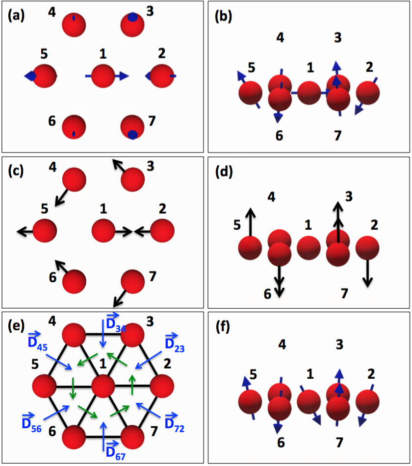
Figure 7: Top (a) and side (b) view of the magnetic ground state configuration for a hexagon made of seven atoms. The projection of the unit vectors of the magnetic moments on the surface plane is given in (c) and along the $z$-axis in (d). The corresponding DM vectors between the nearest neighbors are plotted in (e). In (f) the side view of the ground state after adding a single-ion magnetic anisotropy, $K$, of -6 meV.

V Conclusions

We investigated the complex chiral magnetic behavior of nanostructures of different shapes and sizes wherein the atoms interact via long-range interactions mediated by Rashba electrons. We use an embedding technique based on the Rashba Hamiltonian and the s-wave approximation followed by a mapping procedure to an extended Heisenberg model. The analytical forms of the elements of the tensor of the magnetic exchange interactions is presented within the RKKY-approximation, i.e. without renormalizing the electronic structure because of the presence of the nanostructure. We corrected the forms given by Imamura et al.Imamura et al. (2004), and demonstrate the deep link between the magnetic interaction and the components of the magnetic Friedel oscillations generated by the single adatoms. The isotropic interaction and the DM interactions correspond respectively to the induced out-of-plane and in-plane magnetization. Besides these two interactions, the pseudo-dipolar term, already found in Ref. Imamura et al., 2004, is shown to be large, generating a collinear phase competing with non-collinear structures induced by the DM interaction. We go beyond the RKKY-approximation by considering energy dependent scattering matrices and multiple scattering effects to demonstrate that the size and shape of the nanostructures have a strong impact on the magnitude and sign of the magnetic interactions. We proposed an interesting connection between the DM interaction and the isotropic magnetic exchange interaction, $J$. The DM interaction can be related to the first order change of $J$ with respect to the spin-orbit interaction and even more important, the origin of the sign of the DM interaction, i.e. defining the chirality, can be interpreted by the increase or decrease of $J$ upon application of the spin-orbit interaction. We considered nano-objects that can be built experimentally (see e.g. Refs.Zhu et al. (2011); Khajetoorians et al. (2012, 2016)) and show that each of the objects behave differently and the stability of their non-collinear chiral spin texture is closely connected with the type of structure built on the substrate.

Appendix A

The Green function for the Rashba electron gas can be calculated using the spectral representation:

$$\boldsymbol{G}^{0}(\vec{r},\vec{r}^{\,\prime},E+i\epsilon)=\sum_{\vec{k}n}\frac{\psi_{\vec{k}n}(\vec{r})\,\psi^{*}_{\vec{k}n}(\vec{r}^{\,\prime})}{E-E_{n}+i\epsilon}$$ (30)

Where $E_{n}$ and $\psi_{\vec{k}}(\vec{r})$ are respectively the eigenvalues and eigenstates of the Rashba Hamiltonian. The Rashba Green function is translationally invariant therefore $\boldsymbol{G}^{0}(\vec{r},\vec{r}^{\,\prime},E+i\epsilon)=\boldsymbol{G}^{0}(\vec{R},E+i\epsilon)$, with $\vec{R}=\vec{r}-\vec{r}^{\,\prime}$. After performing the sums over $\vec{k}$ and $n$, the diagonal and off diagonal spin elements of the Green function $\boldsymbol{G}^{0}$ of the Rashba electrons are given as:

$$G_{D}(R,E+i\epsilon)=-\frac{im^{*}}{2\hbar^{2}(k_{1}+k_{2})}\Bigg{[}k_{1}\,H_{0}(k_{1}R+i\epsilon)+k_{2}\,H_{0}(k_{2}R+i\epsilon)\Bigg{]}\quad,$$ (31)

$$G_{ND}(R,E+i\epsilon)=-\frac{im^{*}}{2\hbar^{2}(k_{1}+k_{2})}\Bigg{[}k_{1}\,H_{1}(k_{1}R+i\epsilon)-k_{2}\,H_{1}(k_{2}R+i\epsilon)\Bigg{]}\quad.$$ (32)

As mentioned in the main text, the vectors $k_{1}$ and $k_{2}$ are given by $k_{1}=k_{\mathrm{so}}+\sqrt{k_{\mathrm{so}}^{2}+\frac{2m^{*}E}{\hbar^{2}}}$ and $k_{2}=-k_{\mathrm{so}}+\sqrt{k_{\mathrm{so}}^{2}+\frac{2m^{*}E}{\hbar^{2}}}$ with $k_{\mathrm{so}}=\frac{m^{*}\alpha}{\hbar^{2}}$.

Appendix B

In this appendix we derive the generalized Heisenberg Hamiltonian $H_{ij}=\vec{e}_{i}\,\underline{\underline{{\mathbf{J}}}}_{ij}\,\vec{e}_{j}$, which was simplified to the form given by Eq. 18. For this purpose, we need to calculate the elements of the tensor of exchange interactions showing up in Eq. 16, i.e. $\mathrm{Tr}\,\{\boldsymbol{\sigma}^{\alpha}\,\mathbf{G}_{ij}\,\boldsymbol{\sigma}^{\beta}\,\mathbf{G}_{ji}\}$, considering that $\mathbf{G}$ can be expressed in terms of $G_{D}$ and $G_{ND}$ (see Eq. 17). This can be evaluated via the following trace (omitting the energy integration):

$$\begin{split}H_{ij}&=\mathrm{Tr}\,[(\vec{e}_{i}\cdot\vec{\boldsymbol{\sigma}})(G_{D}\,\boldsymbol{\sigma}_{0}-i\,G_{ND}(\cos\beta\,\boldsymbol{\sigma}_{y}-\sin\beta\,\boldsymbol{\sigma}_{x}))\\ &\hskip 28.45274pt\times(\vec{e}_{j}\cdot\vec{\boldsymbol{\sigma}})(G_{D}\,\boldsymbol{\sigma}_{0}+i\,G_{ND}(\cos\beta\ \boldsymbol{\sigma}_{y}-\sin\beta\hskip 2.84526pt\boldsymbol{\sigma}_{x}))]\quad.\end{split}$$ (33)

Using the properties of the Pauli matrices, we know that for two vectors $\vec{A}$ and $\vec{B}$, the following relation holds: $(\vec{A}\cdot\vec{\boldsymbol{\sigma}})\,(\vec{B}\cdot\vec{\boldsymbol{\sigma}})=(\vec{A}\cdot\vec{B})\ \boldsymbol{\sigma}_{0}+i\,(\vec{A}\times\vec{B})\cdot\vec{\boldsymbol{\sigma}}$. Thus :

$$\begin{split}H_{ij}&=2\,\vec{e}_{i}\cdot\vec{e}_{j}\,(G_{D}^{2}-G_{ND}^{2})-4\,(\vec{e}_{i}\times\vec{e}_{j})_{x}\,i\,G_{D}\,G_{ND}\,\sin\beta\\ &\quad-4\,(\vec{e}_{i}\times\vec{e}_{j})_{y}\,G_{D}\,G_{ND}\,\cos\beta+4\,e_{i}^{y}\,e_{j}^{y}\,G_{ND}^{2}\,\cos^{2}\beta\\ &\quad+4\,e_{i}^{x}\,e_{j}^{x}\,G_{ND}^{2}\,\sin^{2}\beta-2\,(e_{i}^{x}\,e_{j}^{y}+e_{i}^{y}\,e_{j}^{x})\,G_{ND}^{2}\,\sin\beta\,\cos\beta\quad.\end{split}$$ (34)

The terms proportional to $e_{i}^{x}\,e_{j}^{x}$ and $e_{i}^{y}\,e_{j}^{y}$ will lead to the pseudo-dipolar like terms after performing the energy integration given in Eq. 16. The terms proportional to $(e_{i}^{x}\,e_{j}^{y}+e_{i}^{y}\,e_{j}^{x})$ are called interface terms. We can combine both terms in a pseudo-dipolar Hamiltonian for the two-dimensional case;

$$H_{psd}=I\,\sum_{i,j}[(\vec{e}_{i}\cdot\vec{e}_{j})-(\vec{e}_{i}\cdot\vec{R}_{ij})(\vec{e}_{j}\cdot\vec{R}_{ij})-e_{i}^{z}\,e_{j}^{z}]\quad.$$ (35)

$\vec{R}_{ij}$ is the vector connecting the impurities {i, j}.

If we consider that the two magnetic impurities are along the $x$-axis then $\beta=0$ and we get the expression below for the trace:

$$H_{ij}=2\,(G_{D}^{2}-G_{ND}^{2})\,\vec{e}_{i}\cdot\vec{e}_{j}-4\,G_{D}\,G_{ND}\,(\vec{e}_{i}\times\vec{e}_{j})_{y}+4\,G_{ND}^{2}e_{i}^{y}\,e_{j}^{y}\quad,$$ (36)

which leads to the final form of the Hamiltonian given in Eq. 18, and to the identification of the different magnetic interaction terms as presented in Eqs. 22, 23, 25.

Appendix C

In order to obtain the analytical forms of $J$, $D$ and $I$ in the RKKY-approximation (Eqs. 22, 23, 25), we evaluate the integrands needed in Eqs. 19, 20, 21 considering two regimes, positive or negative $k_{1}$. For $k_{1}<0$:

$$G_{D}^{2}=-\frac{(m^{*})^{2}}{4\hbar^{2}(k_{1}+k_{2})^{2}}\hskip 2.84526pt[\hskip 2.84526ptk_{1}^{2}\hskip 2.84526ptH_{0}^{*2}(|k_{1}|R)+k_{2}^{2}\hskip 2.84526ptH_{0}^{2}(k_{2}R)-2\ k_{1}k_{2}\hskip 2.84526ptH^{*}_{0}(|k_{1}|R)H_{0}(k_{2}R)\hskip 2.84526pt]\quad,$$ (37)

$$G_{ND}^{2}=-\frac{(m^{*})^{2}}{4\hbar^{2}(k_{1}+k_{2})^{2}}\hskip 2.84526pt[\hskip 2.84526ptk_{1}^{2}\hskip 2.84526ptH_{1}^{*2}(|k_{1}|R)+k_{2}^{2}\hskip 2.84526ptH_{1}^{2}(k_{2}R)-2\ k_{1}k_{2}\hskip 2.84526ptH^{*}_{1}(|k_{1}|R)H_{1}(k_{2}R)\hskip 2.84526pt]\quad,$$ (38)

and

$$\begin{split}G_{D}G_{ND}&=-\frac{(m^{*})^{2}}{4\hbar^{2}(k_{1}+k_{2})^{2}}\hskip 2.84526pt[\hskip 2.84526pt-k^{2}_{1}\hskip 2.84526ptH^{*}_{0}(|k_{1}|R)H^{*}_{1}(|k_{1}|R)+k_{1}k_{2}\ H_{0}^{*}(|k_{1}|R)H_{1}(k_{2}R)\\ &\hskip 71.13188pt\quad+k_{1}k_{2}\ H_{1}^{*}(|k_{1}|R)H_{0}(k_{2}R)-k_{2}^{2}\hskip 2.84526ptH_{1}(k_{2}R)H_{0}(k_{2}R)\hskip 2.84526pt]\quad.\end{split}$$ (39)

In case $k_{1}>0$:

$$G_{D}^{2}=-\frac{(m^{*})^{2}}{4\hbar^{2}(k_{1}+k_{2})^{2}}\hskip 2.84526pt[\hskip 2.84526ptk_{1}^{2}\hskip 2.84526ptH_{0}^{2}(k_{1}R)+k_{2}^{2}\hskip 2.84526ptH_{0}^{2}(k_{2}R)+2k_{1}k_{2}\hskip 2.84526ptH_{0}(k_{1}R)H_{0}(k_{2}R)\hskip 2.84526pt]\quad,$$ (40)

$$G_{ND}^{2}=-\frac{(m^{*})^{2}}{4\hbar^{2}(k_{1}+k_{2})^{2}}\hskip 2.84526pt[\hskip 2.84526ptk_{1}^{2}\hskip 2.84526ptH_{1}^{2}(k_{1}R)+k_{2}^{2}\hskip 2.84526ptH_{1}^{2}(k_{2}R)-2k_{1}k_{2}\hskip 2.84526ptH_{1}(k_{1}R)H_{1}(k_{2}R)\hskip 2.84526pt]\quad,$$ (41)

and

$$\begin{split}G_{D}\ G_{ND}&=-\frac{(m^{*})^{2}}{4\hbar^{2}(k_{1}+k_{2})^{2}}\hskip 2.84526pt[\hskip 2.84526ptk_{1}^{2}\hskip 2.84526ptH_{0}(k_{1}R)H_{1}(k_{1}R)-k_{1}k_{2}\hskip 2.84526ptH_{0}(k_{1}R)H_{1}(k_{2}R)\\ &\hskip 71.13188pt\quad+k_{1}k_{2}\hskip 2.84526ptH_{1}(k_{1}R)H_{0}(k_{2}R)-k_{2}^{2}\hskip 2.84526ptH_{0}(k_{2}R)H_{1}(k_{2}R)\hskip 2.84526pt]\quad.\end{split}$$ (42)

We use the asymptotic expansion for the Hankel functions for large R: $H_{0}(x)\simeq\sqrt{\frac{2}{\pi x}}\hskip 2.84526pte^{i(x-\frac{\pi}{4})}$ and $H_{1}(x)\simeq\sqrt{\frac{2}{\pi x}}\hskip 2.84526pte^{i(x-\frac{3\pi}{4})}$ which simplify the previous forms for negative $k_{1}<0$ to:

$$G_{D}^{2}=\frac{i(m^{*})^{2}}{2\hbar^{2}(k_{1}+k_{2})^{2}\pi R}\,[-|k_{1}|\,e^{-2i|k_{1}|R}+k_{2}\,e^{2ik_{2}R}+2i\,\sqrt{|k_{1}|k_{2}}\,e^{(k_{2}-|k_{1}|)R}\,]\quad,$$ (43)

$$G_{ND}^{2}=-\frac{i(m^{*})^{2}}{2\hbar^{2}(k_{1}+k_{2})^{2}\pi R}\,[-|k_{1}|\,e^{-2i|k_{1}|R}+k_{2}\,e^{2ik_{2}R}-2i\,\sqrt{|k_{1}|k_{2}}\,e^{(k_{2}-|k_{1}|)R}\,]\quad,$$ (44)

and

$$G_{D}\,G_{ND}=\frac{(m^{*})^{2}}{2\hbar^{2}(k_{1}+k_{2})^{2}\pi R}\,[\,-|k_{1}|\ e^{-2i|k_{1}|R}-k_{2}\,e^{2ik_{2}R}\,]\quad.$$ (45)

While a positive $k_{1}$ leads to:

$$G_{D}^{2}=\frac{i(m^{*})^{2}}{2\hbar^{2}(k_{1}+k_{2})^{2}\pi R}\,[\,k_{1}\,e^{2ik_{1}R}+k_{2}\,e^{2ik_{2}R}+2\sqrt{k_{1}k_{2}}\,e^{i(k_{1}+k_{2})R}\,]\quad,$$ (46)

$$G_{ND}^{2}=-\frac{i(m^{*})^{2}}{2\hbar^{2}(k_{1}+k_{2})^{2}\pi R}\,[\,k_{1}\,e^{2ik_{1}R}+k_{2}\,e^{2ik_{2}R}-2\sqrt{k_{1}k_{2}}\,e^{i(k_{1}+k_{2})R}\,]\quad,$$ (47)

and

$$G_{D}\,G_{ND}=\frac{(m^{*})^{2}}{2\hbar^{2}(k_{1}+k_{2})^{2}\pi R}\,[\,k_{1}\,e^{2ik_{1}R}-k_{2}\,e^{2ik_{2}R}\,]\quad.$$ (48)

From the expressions above we notice that contrary to the terms $(G_{D}^{2}-G_{ND}^{2})$ and $G_{D}\ G_{ND}$, $G_{D}$ and $G_{ND}$ behave differently in the first and second regime.

References

- Dzyaloshinskii (1957) I. E. Dzyaloshinskii, “Thermodynamic theory of weak ferromagnetism in antiferromagnetic substances,” Sov. Phys. JETP 5, 1259 (1957).
- Moriya (1960) T. Moriya, “Anisotropic superexchange interaction and weak ferromagnetism,” Phys. Rev. 120, 91 (1960).
- Bode et al. (2007) M. Bode, M. Heide, K. von Bergmann, P. Ferriani, S. Heinze, G. Bilhmayer, A. Kubetzka, O. Pietzsch, S. Blügel, and R. Wiesendanger, “Chiral magnetic order at surfaces driven by inversion asymmetry,” Nature 447, 190–193 (2007).
- Ferriani et al. (2008) P. Ferriani, K. von Bergmann, E. Y. Vedmedenko, S. Heinze, M. Bode, M. Heide, G. Bihlmayer, S. Blügel, and R. Wiesendanger, “Atomic-scale spin spiral with a unique rotational sense: Mn monolayer on W(001),” Phys. Rev. Lett. 101, 027201 (2008).
- Santos et al. (2008) B Santos, J M Puerta, J I Cerda, R Stumpf, K von Bergmann, R Wiesendanger, M Bode, K F McCarty, and J de la Figuera, “Structure and magnetism of ultra-thin chromium layers on W(110),” New Journal of Physics 10, 013005 (2008).
- Schweflinghaus et al. (2016) B. Schweflinghaus, B. Zimmermann, G. Heide, G. Bihlmayer, and S. Blügel, “Role of Dzyaloshinskii-Moriya interaction for magnetism in transition-metal chains at Pt step-edges,” arXiv: , 1511.02469 (2016).
- Menzel et al. (2012) Matthias Menzel, Yuriy Mokrousov, Robert Wieser, Jessica E. Bickel, Elena Vedmedenko, Stefan Blügel, Stefan Heinze, Kirsten von Bergmann, André Kubetzka, and Roland Wiesendanger, “Information transfer by vector spin chirality in finite magnetic chains,” Phys. Rev. Lett. 108, 197204 (2012).
- Khajetoorians et al. (2016) A. A. Khajetoorians, M. Steinbrecher, M. Ternes, M. Bouhassoune, M. dos Santos Dias, S. Lounis, J. Wiebe, and R. Wiesendanger, “Tailoring the chiral magnetic interaction between two individual atoms,” Nature Communications 7, 10620 (2016).
- Mankovsky et al. (2009) S. Mankovsky, S. Bornemann, J. Minár, S. Polesya, H. Ebert, J. B. Staunton, and A. I. Lichtenstein, “Effects of spin-orbit coupling on the spin structure of deposited transition-metal clusters,” Phys. Rev. B 80, 014422 (2009).
- Antal et al. (2008) A. Antal, B. Lazarovits, L. Udvardi, L. Szunyogh, B. Újfalussy, and P. Weinberger, “First-principles calculations of spin interactions and the magnetic ground states of Cr trimers on Au(111),” Phys. Rev. B 77, 174429 (2008).
- Mühlbauer et al. (2009) S. Mühlbauer, B. Binz, F. Jonietz, C. Pfleiderer, A. Rosch, A. Neubauer, R. Georgii, and P. Böni, “Skyrmion lattice in a chiral magnet,” Science 323, 915–919 (2009).
- Yu et al. (2010) X. Z. Yu, Y. Onose, N. Kanazawa, J. H. Park, J. H. Han, Y. Matsui, N. Nagaosa, and Y. Tokura, “Real-space observation of a two-dimensional skyrmion crystal,” Nature 465, 901–904 (2010).
- Romming et al. (2013) Niklas Romming, Christian Hanneken, Matthias Menzel, Jessica E. Bickel, Boris Wolter, Kirsten von Bergmann, André Kubetzka, and Roland Wiesendanger, “Writing and deleting single magnetic skyrmions,” Science 341, 636–639 (2013).
- Heinze et al. (2011) S. Heinze, K. von Bergmann, M. Menzel, J. Brede, A. Kubetzka, Wiesendanger R., G. Bihlmayer, and S. Blügel, “Spontaneous atomic-scale magnetic skyrmion lattice in two dimensions,” Nat. Phys. 7, 713–718 (2011).
- Bogdanov and Yablonskii (1989) A. N. Bogdanov and D. A. Yablonskii, “Thermodynamically stable ‘vortices’ in magnetically ordered crystals. the mixed state of magnets,” Sov. Phys. JETP 68, 101–103 (1989).
- Roessler et al. (2006) U. K. Roessler, A. N. Bogdanov, and C. Pfleiderer, “Spontaneous skyrmion ground states in magnetic metals,” Nature 442, 797–801 (2006).
- Baibich et al. (1988) M. N. Baibich, J. M. Broto, A. Fert, F. Nguyen Van Dau, F. Petroff, P. Etienne, G. Creuzet, A. Friederich, and J. Chazelas, “Giant magnetoresistance of (001)Fe/(001)Cr magnetic superlattices,” Phys. Rev. Lett. 61, 2472–2475 (1988).
- Crum et al. (2015) D. M. Crum, M. Bouhassoune, J. Bouaziz, B. Schweflinghaus, S. Blügel, and S. Lounis, “Perpendicular reading of single confined magnetic skyrmions,” Nature Communications 6, 8541 (2015).
- Hanneken et al. (2015) C. Hanneken, F. Otte, A. Kubetzka, B. Dupé, N. Romming, K. von Bergmann, R. Wiesendanger, and S. Heinze, “Electrical detection of magnetic skyrmions by tunnelling non-collinear magnetoresistance,” Nat. Nanotech. 10, 1039–1042 (2015).
- Hamamoto et al. (2016) K. Hamamoto, M. Ezawa, and N. Nagaosa, “Purely electrical detection of a skyrmion in constricted geometry,” Appl. Phys. Lett. 108, 112401 (2016).
- Jonietz et al. (2010) F. Jonietz, S. Mühlbauer, C. Pfleiderer, A. Neubauer, W. Münzer, A. Bauer, T. Adams, R. Georgii, P. Böni, R. A. Duine, K. Everschor, M. Garst, and A. Rosch, “Spin transfer torques in MnSi at ultralow current densities,” Science 330, 1648–1651 (2010).
- Parkin et al. (2008) Stuart S. P. Parkin, Masamitsu Hayashi, and Luc Thomas, “Magnetic domain-wall racetrack memory,” Science 320, 190–194 (2008).
- Smith (1976) D. A. Smith, “New mechanisms for magnetic anisotropy in localised s-state moment materials,” J. Magn. Magn. Mater. 1, 214–225 (1976).
- Fert and Levy (1980) A. Fert and P. M. Levy, “Role of anisotropic exchange interactions in determining the properties of spin-glasses,” Phys. Rev. Lett. 44, 1538–1541 (1980).
- Ruderman and Kittel (1954) M. A. Ruderman and C. Kittel, “Indirect exchange coupling of nuclear magnetic moments by conduction electrons,” Phys. Rev. 96, 99–102 (1954).
- Kasuya (1956) T. Kasuya, “A theory of metallic ferro- and antiferromagnetism on zener’s model,” Prog. Theor. Phys. 16, 45–57 (1956).
- Yosida (1957) K. Yosida, “Magnetic properties of Cu–Mn alloys,” 106, 893–898 (1957).
- Zhou et al. (2010) L. Zhou, J. Wiebe, S. Lounis, E. Vedmedenko, F. Meier, S. Blügel, P. H. Dederichs, and R. Wiesendanger, “Strength and directionality of surface Ruderman–Kittel–Kasuya–Yosida interaction mapped on the atomic scale,” Nat. Phys. 6, 187–191 (2010).
- Khajetoorians et al. (2012) A. A. Khajetoorians, J. Wiebe, B. Chilian, S. Lounis, S. Blügel, and R. Wiesendanger, “Atom-by-atom engineering and magnetometry of tailored nanomagnets,” Nat. Phys. 8, 497–503 (2012).
- Prüser et al. (2014) H. Prüser, P. E. Dargel, M. Bouhassoune, Ulbrich R. G., T. Pruschke, S. Lounis, and M. Wenderoth, “Interplay between the Kondo effect and the Ruderman–Kittel-Kasuya–Yosida interaction,” Nature Communications 5, 5417 (2014).
- Imamura et al. (2004) Hiroshi Imamura, Patrick Bruno, and Yasuhiro Utsumi, “Twisted exchange interaction between localized spins embedded in a one- or two-dimensional electron gas with Rashba spin-orbit coupling,” Phys. Rev. B 69, 121303 (2004).
- Rashba (1960) E. I. Rashba, “Svoistva poluprovodnikov s petlei ekstremumov. i. tsiklotronnyi i kombinirovannyi rezonans v magnitnom pole, perpendikulyarnom ploskosti petli, fizika tverd. tela.” Sov. Phys. Solid State 2, 1109 (1960).
- Bychkov and I. (1984) Y. A. Bychkov and Rashba E. I., “Svoistva dvumernogo elektronnogo gaza so snyatym vyrozhdeniem spektra,” J. Phys. C: Solid State Phys. 17, 6039 (1984).
- Zhu et al. (2011) Jia-Ji Zhu, Dao-Xin Yao, Shou-Cheng Zhang, and Kai Chang, “Electrically controllable surface magnetism on the surface of topological insulators,” Phys. Rev. Lett. 106, 097201 (2011).
- LaShell et al. (1996) S. LaShell, B. A. McDougall, and E. Jensen, “Spin splitting of an Au(111) surface state band observed with angle resolved photoelectron spectroscopy,” Phys. Rev. Lett. 77, 3419–3422 (1996).
- Lounis et al. (2012) Samir Lounis, Andreas Bringer, and Stefan Blügel, “Magnetic adatom induced skyrmion-like spin texture in surface electron waves,” Phys. Rev. Lett. 108, 207202 (2012).
- Walls and Heller (2007) Jamie D. Walls and Eric J. Heller, “Spin-orbit coupling induced interference in quantum corrals,” Nano Letters 7, 3377–3382 (2007).
- Fiete and Heller (2003) Gregory A. Fiete and Eric J. Heller, “Colloquium : Theory of quantum corrals and quantum mirages,” Rev. Mod. Phys. 75, 933–948 (2003).
- Lloyd and Smith (1972) P. Lloyd and P.V. Smith, “Multiple scattering theory in condensed materials,” Advances in Physics 21, 69–142 (1972).
- Liechtenstein et al. (1987) A.I. Liechtenstein, M.I. Katsnelson, V.P. Antropov, and V.A. Gubanov, “Local spin density functional approach to the theory of exchange interactions in ferromagnetic metals and alloys,” Journal of Magnetism and Magnetic Materials 67, 65 – 74 (1987).
- Udvardi et al. (2003) L. Udvardi, L. Szunyogh, K. Palotás, and P. Weinberger, “First-principles relativistic study of spin waves in thin magnetic films,” Phys. Rev. B 68, 104436 (2003).
- Ebert and Mankovsky (2009) H. Ebert and S. Mankovsky, “Anisotropic exchange coupling in diluted magnetic semiconductors: Ab initio spin-density functional theory,” Phys. Rev. B 79, 045209 (2009).
- Bouaziz et al. (2016) J. Bouaziz, S. Lounis, S. Blügel, and H. Ishida, “Microscopic theory of the residual surface resistivity of rashba electrons,” Phys. Rev. B 94, 045433 (2016).
- Šipr et al. (2016) O. Šipr, S. Mankovsky, S. Polesya, S. Bornemann, J. Minár, and H. Ebert, “Illustrative view on the magnetocrystalline anisotropy of adatoms and monolayers,” Phys. Rev. B 93, 174409 (2016).
- Kim et al. (2013) Kyoung-Whan Kim, Hyun-Woo Lee, Kyung-Jin Lee, and M. D. Stiles, “Chirality from interfacial spin-orbit coupling effects in magnetic bilayers,” Phys. Rev. Lett. 111, 216601 (2013).
- Lounis (2014) S. Lounis, “Non-collinear magnetism induced by frustration in transition-metal nanostructures deposited on surfaces,” Journal of Physics: Condensed Matter 26, 273201 (2014).