Impact of scalar leptoquarks on heavy baryonic decays

Abstract

We present a study on the impact of scalar leptoquarks on the semileptonic decays of $\Lambda_{b}$, $\Sigma_{b}$ and $\Xi_{b}$. To this end, we calculate the differential branching ratio and lepton forward-backward asymmetry defining the processes $\Lambda_{b}\rightarrow\Lambda\ell^{+}\ell^{-}$, $\Sigma_{b}\rightarrow\Sigma\ell^{+}\ell^{-}$ and $\Xi_{b}\rightarrow\Xi\ell^{+}\ell^{-}$, with $\ell$ being $\mu$ or $\tau$, using the form factors calculated via light cone QCD in full theory. In calculations, the errors of form factors are taken into account. We compare the results obtained in leptoquark model with those of the standard model as well as the existing lattice QCD predictions and experimental data.

I Introduction

The physics of transitions based on $b\rightarrow s\ell^{+}\ell^{-}$ at quark level constitutes one of the main directions of the research in high energy and particle physics both theoretically and experimentally as new physics effects can contribute to such decay channels. The flavor changing neutral current (FCNC) transitions of $\Lambda_{b}\rightarrow\Lambda\ell^{+}\ell^{-}$, $\Sigma_{b}\rightarrow\Sigma\ell^{+}\ell^{-}$ and $\Xi_{b}\rightarrow\Xi\ell^{+}\ell^{-}$ are among important baryonic decay channels that can be used as sensitive probes to indirectly search for new physics contributions. Especially, the rare $\Lambda_{b}\rightarrow\Lambda\ell^{+}\ell^{-}$ decay channel has been in the focus of much attention in recent years both theoretically and experimentally. The first measurement on the $\Lambda_{b}\rightarrow\Lambda\mu^{+}\mu^{-}$ process has been reported by the CDF Collaboration Aaltonen:2011qs with $24$ signal events and a statistical significance of $5.8$ Gaussian standard deviations. Using the $p\overline{p}$ collisions data samples corresponding to $6.8fb^{-1}$ and $\sqrt{s}=1.96$ TeV collected by the CDF II detector, the differential branching ratio for the $\Lambda_{b}\rightarrow\Lambda\mu^{+}\mu^{-}$ decay channel has been measured to be $dBr(\Lambda_{b}^{0}\rightarrow\Lambda\mu^{+}\mu^{-})/dq^{2}=[1.73\pm 0.42(stat)\pm 0.55(syst)]\times 10^{-6}$ Aaltonen:2011qs . The differential branching fraction of $\Lambda_{b}^{0}\rightarrow\Lambda\mu^{+}\mu^{-}$ decay channel has also been measured as $dBr(\Lambda_{b}^{0}\rightarrow\Lambda\mu^{+}\mu^{-})/dq^{2}=(1.18\;^{+\,0.09}_{-\,0.08}\pm 0.03\pm 0.27)\times 10^{-7}$ GeV${}^{2}/$c⁴ at $15$ GeV${}^{2}/$c${}^{4}\leq$ $q^{2}\leq 20$ GeV${}^{2}/$c⁴ region by the LHCb Collaboration LHCb . The LHCb Collaboration has also measured the lepton forward-backward asymmetries associated to this transition as $A_{FB}^{\mu}=-0.05\pm 0.09(stat)\pm 0.03(syst)$ at $15$ GeV${}^{2}/$c${}^{4}\leq$ $q^{2}\leq 20$ GeV${}^{2}/$c⁴ region LHCb . The order of branching ratio in $\Lambda_{b}\rightarrow\Lambda e^{+}e^{-}$, $\Lambda_{b}\rightarrow\Lambda\tau^{+}\tau^{-}$ as well as in $\Sigma_{b}\rightarrow\Sigma\ell^{+}\ell^{-}$ and $\Xi_{b}\rightarrow\Xi\ell^{+}\ell^{-}$ (for all leptons) indicates that these channels are all accessible at LHC (for details see Refs.Aliev:2010uy ; Azizi:2011if ; Azizi:2011mw ; Azizi:2012yg ; Azizi:2013eta ) . We hope with the RUN II data at the center of mass energy 13 TeV it will be possible to measure different physical quantities related to these FCNC loop level rare transitions in near future.

The LHC RUN II may provide opportunities to search for various new physics scenarios. One of the important new physics models that has been proposed to overcome the problems of some inconsistencies between the SM predictions and experimental data, is the leptoquark (LQ) model. Hereafter, by LQ model we mean a minimal renormalizable scalar leptoquark model which will be explained in some details in next section. As an example for the LHC constraints and prospects for scalar leptoquarks explaining the $\overline{B}\rightarrow D^{(*)}\tau\overline{\nu}$ anomaly see Dumont:2016xpj . LQs are hypothetical color triplet bosons that couple to leptons and quarks pdg . LQs carry both baryon (B) and lepton (L) quantum numbers with color and electric charges. The spin number of a leptoquark state can be $0$ or $1$, corresponding to a scalar leptoquark or vector leptoquark. If the leptoquarks violate both the baryon and lepton numbers, they are generally considered to be heavy particles at the level of ${\cal O}(10^{15})$ GeV in order to prevent the proton decay. For more detailed information about leptoquark models and the recent experimental and theoretical progresses, see Dorsner:2016wpm ; Davidson:1993qk ; Hewett:1997ce ; Shanker:1981mj ; Fajfer:2008tm ; Saha:2010vw ; Davidson:2011zn ; Kosnik:2012dj ; Arnold:2013cva ; Sakaki:2013bfa ; Mohanta:2013lsa ; Allanach:2015ria ; Sahoo:2015wya ; Sahoo:2015qha ; Sahoo:2015fla ; Sahoo:2015pzk ; Kumar:2016omp ; Dorsner:2009cu ; Dorsner:2011ai ; Becirevic:2016oho ; Becirevic:2016yqi .

In the light of progresses about LQs, we calculate the differential branching ratio and lepton forward-backward asymmetry corresponding to the $\Lambda_{b}\rightarrow\Lambda\ell^{+}\ell^{-}$, $\Sigma_{b}\rightarrow\Sigma\ell^{+}\ell^{-}$ and $\Xi_{b}\rightarrow\Xi\ell^{+}\ell^{-}$ processes in a scalar LQ model. In the calculations, we use the form factors as the main inputs calculated from the light cone QCD sum rules in full theory. We also encounter the errors of the form factors to the calculations. We compare the regions swept by the LQ model with those of the SM and search for deviations of the LQ model predictions with those of the SM. We also compare the results with the available lattice predictions and experimental data.

The outline of this article is as follow. In next section, we present the effective Hamiltonian responsible for the transitions under consideration both in the SM and LQ models. In section III, we present the transition amplitude and matrix elements defining the above transitions. In section IV, we calculate the differential decay rate and the lepton forward-backward asymmetry in the baryonic $\Lambda_{b}\rightarrow\Lambda\ell^{+}\ell^{-}$, $\Sigma_{b}\rightarrow\Sigma\ell^{+}\ell^{-}$ and $\Xi_{b}\rightarrow\Xi\ell^{+}\ell^{-}$ channels and numerically analyze the results obtained. We compare the LQ predictions with those of the SM and existing lattice results and experimental data also in this section.

II The Effective Hamiltonian and Wilson Coefficients

At the quark level the effective Hamiltonian, defining the above mentioned $b\rightarrow s\ell^{+}\ell^{-}$ based transitions, in terms of Wilson coefficients and different operators in SM is generally defined as Buchalla:1995vs ; Altmannshofer:2008dz

$${\cal H}^{eff}_{SM} = {G_{F}\alpha_{em}V_{tb}V_{ts}^{\ast}\over 2\sqrt{2}\pi}\Bigg{[}C^{eff}_{9}\bar{s}\gamma_{\mu}(1-\gamma_{5})b\,\bar{\ell}\gamma^{\mu}\ell$$ (1)

$$+ C^{\prime~{}eff}_{9}\bar{s}\gamma_{\mu}(1+\gamma_{5})b\,\bar{\ell}\gamma^{\mu}\ell$$

$$+ C_{10}\bar{s}\gamma_{\mu}(1-\gamma_{5})b\,\bar{\ell}\gamma^{\mu}\gamma_{5}\ell$$

$$+ C^{\prime}_{10}\bar{s}\gamma_{\mu}(1+\gamma_{5})b\,\bar{\ell}\gamma^{\mu}\gamma_{5}\ell$$

$$- 2m_{b}C^{eff}_{7}{1\over q^{2}}\bar{s}i\sigma_{\mu\nu}q^{\nu}(1+\gamma_{5})b\,\bar{\ell}\gamma^{\mu}\ell$$

$$- 2m_{b}C^{\prime~{}eff}_{7}{1\over q^{2}}\bar{s}i\sigma_{\mu\nu}q^{\nu}(1-\gamma_{5})b\,\bar{\ell}\gamma^{\mu}\ell\Bigg{]}~{},$$

where $G_{F}$ is the Fermi weak coupling constant, $\alpha_{em}$ is the fine structure constant at $Z$ mass scale, $V_{tb}$ and $V_{ts}^{\ast}$ are elements of the Cabibbo-Kobayashi-Maskawa (CKM) matrix, the $C^{(\prime)~{}eff}_{9}$, $C^{(\prime)}_{10}$ and $C^{(\prime)~{}eff}_{7}$ are the SM Wilson coefficients and $q^{2}$ is the transferred momentum squared. Here the superscript “eff” refers to the shifts in the corresponding coefficients due to the effects of four-quark operators at large $q^{2}$. The primed coefficients are ignored since the Hamiltonian does not receive any contribution from the corresponding operators in the SM. We collect the explicit expressions of the Wilson coefficients $C^{eff}_{9}$, $C_{10}$ and $C^{eff}_{7}$ in the Appendix: A.

Considering the additional contributions arising from the exchange of scalar leptoquarks, the effective Hamiltonian is modified. The modified Hamiltonian in LQ model is obtained from Eq. (1) by the replacements $C^{eff}_{9}\rightarrow C^{eff,tot}_{9}$, $C^{\prime~{}eff}_{9}\rightarrow C^{\prime~{}eff,tot}_{9}$, $C_{10}\rightarrow C^{tot}_{10}$ and $C^{\prime}_{10}\rightarrow C^{\prime~{}tot}_{10}$. Here, $C^{eff,tot}_{9}$, $C^{\prime~{}eff,tot}_{9}$, $C^{tot}_{10}$ and $C^{\prime~{}tot}_{10}$, with the superscript “tot” being referring to “total” , are new Wilson coefficients. These coefficients contain contributions from both the SM and LQ models. Note that the Wilson coefficients $C^{eff}_{7}$ and $C^{\prime~{}eff}_{7}$ remain unchanged compared to the SM. The new Wilson coefficients are given as (for details see for instance Mohanta:2013lsa ; Sahoo:2015wya ; Sahoo:2015qha ; Sahoo:2015pzk ; Sahoo:2015fla )

$$C^{eff,tot}_{9} = C^{eff}_{9}+C^{LQ}_{9}~{},$$

$$C^{\prime~{}eff,tot}_{9} = C^{\prime~{}eff}_{9}+C^{\prime~{}LQ}_{9}~{},$$

$$C^{tot}_{10} = C_{10}+C^{LQ}_{10}~{},$$

$$C^{\prime~{}tot}_{10} = C^{\prime}_{10}+C^{\prime~{}LQ}_{10},$$ (2)

where the coefficients $C^{LQ}_{9}$ and $C^{LQ}_{10}$ receive contributions from the exchange of the scalar leptoquarks $X^{(7/6)}=(3,2,7/6)$ but the primed Wilson coefficients $C^{\prime~{}LQ}_{9}$ and $C^{\prime~{}LQ}_{10}$ pick up contributions from the exchange of the scalar leptoquarks $X^{(1/6)}=(3,2,1/6)$. Here we should remark that we consider the effects of the above two scalar leptoquarks on the Wilson coefficients since this representation does not allow proton decay at tree-level. We do not consider the effects of the vector leptoquarks on the processes under consideration. Hence, in the present study we consider the minimal renormalizable scalar leptoquark models including one single additional representation of $SU(3)\times SU(2)\times U(1)$ which guarantees that the proton does not decay. This requisite can only be satisfied by the models that have the representation of $X^{(7/6)}=(3,2,7/6)$ and $X^{(1/6)}=(3,2,1/6)$ scalar leptoquarks under the above gauge group (for details see for instance Arnold:2013cva ; Sahoo:2015wya ).

Thus the coefficients $C^{LQ}_{9}$ and $C^{LQ}_{10}$ are obtained as Mohanta:2013lsa ; Sahoo:2015wya ; Sahoo:2015qha ; Sahoo:2015pzk ; Sahoo:2015fla

$$C^{LQ}_{9}=C^{LQ}_{10}=-\frac{\pi}{2\sqrt{2}G_{F}\alpha_{em}V_{tb}V_{ts}^{*}}\frac{\lambda_{e}^{23}\lambda_{e}^{22*}}{M_{Y}^{2}}\;,$$ (3)

and the primed Wilson coefficients $C^{\prime~{}LQ}_{9}$ and $C^{\prime~{}LQ}_{10}$ are found as Mohanta:2013lsa ; Sahoo:2015wya ; Sahoo:2015qha ; Sahoo:2015pzk ; Sahoo:2015fla

$$C^{\prime~{}LQ}_{9}=-C^{\prime~{}LQ}_{10}=\frac{\pi}{2\sqrt{2}~{}G_{F}\alpha_{em}V_{tb}V_{ts}^{*}}\frac{\lambda_{s}^{22}\lambda_{b}^{32*}}{M_{V}^{2}}\;,$$ (4)

where $Y$ and $V$ are the two components of doublet LQ, $X=(V_{\alpha},Y_{\alpha})$, with $M_{Y}$ and ${M_{V}}$ being representing the masses of the components of the scalar leptoquarks (for details on the LQ interaction Lagrangian and corresponding notations see Sahoo:2016nvx ). It is assumed that each individual leptoquark contribution to the branching ratio does not exceed the experimental result. Here

$$0\leq\left|\frac{\lambda_{e}^{23}\lambda_{e}^{22*}}{M_{Y}^{2}}\right|=\left|\frac{\lambda_{s}^{22}\lambda_{b}^{32*}}{M_{V}^{2}}\right|\leq 5\times 10^{-9}~{}{\rm GeV}^{-2}\;,$$ (5)

obtained via the fitting of the model parameters to the $B_{s}\rightarrow\mu^{+}\mu^{-}$ data Sahoo:2016nvx . In Eq. (5) we assummed that the contributions of the two components $Y$ and $V$ are equal.

III Transition amplitude and matrix elements

Generally, the amplitude of the transition responsible for the $\Lambda_{b}\rightarrow\Lambda\ell^{+}\ell^{-}$, $\Sigma_{b}\rightarrow\Sigma\ell^{+}\ell^{-}$ and $\Xi_{b}\rightarrow\Xi\ell^{+}\ell^{-}$ baryonic decays is provided with sandwiching the effective Hamiltonian between the initial and final baryonic states,

$${\cal M}^{{\cal B}_{Q}\rightarrow{\cal B}\ell^{+}\ell^{-}}=\langle{\cal B}(p)\mid{\cal H}^{eff}\mid{\cal B}_{Q}(p+q,s)\rangle~{},$$ (6)

where ${\cal B}$ represents $\Lambda$, $\Sigma$ and $\Xi$ baryons and $Q$ corresponds to $b$ quark. To get the transition amplitude, we need to consider the following transition matrix elements parametrized in terms of twelve form factors in full QCD, i.e., without any expansion in the heavy quark mass or large hadron energies:

$$\langle{\cal B}(p)\mid\bar{s}\gamma_{\mu}(1 - \gamma_{5})b\mid{\cal B}_{Q}(p+q,s)\rangle=$$

$$\bar{u}_{\cal B}(p)\Bigg{[}\gamma_{\mu}f_{1}(q^{2})+{i}\sigma_{\mu\nu}q^{\nu}f_{2}(q^{2})$$

$$+q^{\mu}f_{3}(q^{2})-\gamma_{\mu}\gamma_{5}g_{1}(q^{2})$$

$$-{i}\sigma_{\mu\nu}\gamma_{5}q^{\nu}g_{2}(q^{2})$$

$$-q^{\mu}\gamma_{5}g_{3}(q^{2})\vphantom{\int_{0}^{x_{2}}}\Bigg{]}u_{{\cal B}_{Q}}(p+q,s)~{},$$

$$\langle{\cal B}(p)\mid\bar{s}\gamma_{\mu}(1 + \gamma_{5})b\mid{\cal B}_{Q}(p+q,s)\rangle=$$

$$\bar{u}_{\cal B}(p)\Bigg{[}\gamma_{\mu}f_{1}(q^{2})+{i}\sigma_{\mu\nu}q^{\nu}f_{2}(q^{2})$$

$$+q^{\mu}f_{3}(q^{2})+\gamma_{\mu}\gamma_{5}g_{1}(q^{2})$$

$$+{i}\sigma_{\mu\nu}\gamma_{5}q^{\nu}g_{2}(q^{2})$$

$$+q^{\mu}\gamma_{5}g_{3}(q^{2})\vphantom{\int_{0}^{x_{2}}}\Bigg{]}u_{{\cal B}_{Q}}(p+q,s)~{},$$

$$\langle{\cal B}(p)\mid\bar{s}i\sigma_{\mu\nu}q^{\nu}(1 + \gamma_{5})b\mid{\cal B}_{Q}(p+q,s)\rangle=$$

$$\bar{u}_{\cal B}(p)\Bigg{[}\gamma_{\mu}f_{1}^{T}(q^{2})+{i}\sigma_{\mu\nu}q^{\nu}f_{2}^{T}(q^{2})$$

$$+q^{\mu}f_{3}^{T}(q^{2})+\gamma_{\mu}\gamma_{5}g_{1}^{T}(q^{2})$$

$$+{i}\sigma_{\mu\nu}\gamma_{5}q^{\nu}g_{2}^{T}(q^{2})$$

$$+q^{\mu}\gamma_{5}g_{3}^{T}(q^{2})\vphantom{\int_{0}^{x_{2}}}\Bigg{]}u_{{\cal B}_{Q}}(p+q,s)~{},$$

$$\langle{\cal B}(p)\mid\bar{s}i\sigma_{\mu\nu}q^{\nu}(1 - \gamma_{5})b\mid{\cal B}_{Q}(p+q,s)\rangle=$$

$$\bar{u}_{\cal B}(p)\Bigg{[}\gamma_{\mu}f_{1}^{T}(q^{2})+{i}\sigma_{\mu\nu}q^{\nu}f_{2}^{T}(q^{2})$$

$$+q^{\mu}f_{3}^{T}(q^{2})-\gamma_{\mu}\gamma_{5}g_{1}^{T}(q^{2})$$

$$-{i}\sigma_{\mu\nu}\gamma_{5}q^{\nu}g_{2}^{T}(q^{2})$$

$$-q^{\mu}\gamma_{5}g_{3}^{T}(q^{2})\vphantom{\int_{0}^{x_{2}}}\Bigg{]}u_{{\cal B}_{Q}}(p+q,s)~{},$$

where the $u_{{\cal B}_{Q}}$ and ${u}_{\cal B}$ represent spinors of the initial and final states, respectively. The $f^{(T)}_{i}$ and $g^{(T)}_{i}$ ($i$ running from $1$ to $3$) are transition form factors . The values of these form factors corresponding to $\Lambda_{b}\rightarrow\Lambda\ell^{+}\ell^{-}$, $\Sigma_{b}\rightarrow\Sigma\ell^{+}\ell^{-}$ and $\Xi_{b}\rightarrow\Xi\ell^{+}\ell^{-}$ transitions and calculated via light cone sum rules in full theory are taken from Aliev:2010uy , Azizi:2011if and Azizi:2011mw , respectively (for form factors of $\Lambda_{b}$ channel calculated with different phenomenological models see also for instance Feldmann:2011xf ; Boer:2014kda ; Wang:2015ndk ). These form factors are also available in lattice QCD in $\Lambda$ channel Detmold:2016pkz .

Using the above transition matrix elements in terms of form factors, we get the amplitude of the transitions $\Lambda_{b}\rightarrow\Lambda\ell^{+}\ell^{-}$, $\Sigma_{b}\rightarrow\Sigma\ell^{+}\ell^{-}$ and $\Xi_{b}\rightarrow\Xi\ell^{+}\ell^{-}$ in the SM and LQ as

$${\cal M}_{SM}^{{\cal B}_{Q}\rightarrow{\cal B}\ell^{+}\ell^{-}} = {G_{F}\alpha_{em}V_{tb}V_{ts}^{\ast}\over 2\sqrt{2}\pi}\Bigg{\{}\Big{[}{\bar{u}}_{\cal B}(p)(\gamma_{\mu}[{\cal A}_{1}^{SM}R+{\cal B}_{1}^{SM}L]+{i}\sigma_{\mu\nu}q^{\nu}[{\cal A}_{2}^{SM}R+{\cal B}_{2}^{SM}L]$$

$$+ q^{\mu}[{\cal A}_{3}^{SM}R+{\cal B}_{3}^{SM}L])u_{{\cal B}_{Q}}(p+q,s)\Big{]}\,(\bar{\ell}\gamma^{\mu}\ell)$$

$$+ \Big{[}{\bar{u}}_{\cal B}(p)(\gamma_{\mu}[{\cal D}_{1}^{SM}R+{\cal E}_{1}^{SM}L]+{i}\sigma_{\mu\nu}q^{\nu}[{\cal D}_{2}^{SM}R+{\cal E}_{2}^{SM}L]$$

$$+ q^{\mu}[{\cal D}_{3}^{SM}R+{\cal E}_{3}^{SM}L])u_{{\cal B}_{Q}}(p+q,s)\Big{]}\,(\bar{\ell}\gamma^{\mu}\gamma_{5}\ell)\Bigg{\}},~{}$$

and

$${\cal M}_{tot}^{{\cal B}_{Q}\rightarrow{\cal B}\ell^{+}\ell^{-}} = {G_{F}\alpha_{em}V_{tb}V_{ts}^{\ast}\over 2\sqrt{2}\pi}\Bigg{\{}\Big{[}{\bar{u}}_{\cal B}(p)(\gamma_{\mu}[{\cal A}_{1}^{tot}R+{\cal B}_{1}^{tot}L]+{i}\sigma_{\mu\nu}q^{\nu}[{\cal A}_{2}^{tot}R+{\cal B}_{2}^{tot}L]$$

$$+ q^{\mu}[{\cal A}_{3}^{tot}R+{\cal B}_{3}^{tot}L])u_{{\cal B}_{Q}}(p+q,s)\Big{]}\,(\bar{\ell}\gamma^{\mu}\ell)$$

$$+ \Big{[}{\bar{u}}_{\cal B}(p)(\gamma_{\mu}[{\cal D}_{1}^{tot}R+{\cal E}_{1}^{tot}L]+{i}\sigma_{\mu\nu}q^{\nu}[{\cal D}_{2}^{tot}R+{\cal E}_{2}^{tot}L]$$

$$+ q^{\mu}[{\cal D}_{3}^{tot}R+{\cal E}_{3}^{tot}L])u_{{\cal B}_{Q}}(p+q,s)\Big{]}\,(\bar{\ell}\gamma^{\mu}\gamma_{5}\ell)\Bigg{\}}~{},$$

where $R=(1+\gamma_{5})/2$ and $L=(1-\gamma_{5})/2$ and the calligraphic coefficients are collected in Appendix: B.

IV Physical Observables

In this section we would like to calculate some physical observables such as the differential decay width, the differential branching ratio and the lepton forward-backward asymmetry for the considered decay channels.

IV.1 The differential decay width

Using the decay amplitudes and transition matrix elements in terms of form factors, we find the differential decay rate defining the transitions under consideration in the LQ model as

$$\frac{d^{2}\Gamma_{tot}}{d\hat{s}dz}(z,\hat{s}) = \frac{G_{F}^{2}\alpha^{2}_{em}m_{{\cal B}_{Q}}}{16384\pi^{5}}|V_{tb}V_{ts}^{*}|^{2}v\sqrt{\lambda(1,r,\hat{s})}\,$$

$$\Bigg{[} {\cal T}_{0}^{tot}(\hat{s})+{\cal T}_{1}^{tot}(\hat{s})z+{\cal T}_{2}^{tot}(\hat{s})z^{2}\Bigg{]}~{},$$

where $v=\sqrt{1-\frac{4m_{\ell}^{2}}{q^{2}}}$ is the lepton velocity, $\lambda=\lambda(1,r,\hat{s})=(1-r-\hat{s})^{2}-4r\hat{s}$ is the usual triangle function, $\hat{s}=q^{2}/m^{2}_{{\cal B}_{Q}}$, $r=m^{2}_{{\cal B}}/m^{2}_{{\cal B}_{Q}}$ and $z=\cos\theta$ with $\theta$ being the angle between momenta of the lepton $l^{+}$ and the ${\cal B}_{Q}$ in the center of mass of leptons. The calligraphic ${\cal T}_{0}^{tot}(\hat{s})$, ${\cal T}_{1}^{tot}(\hat{s})$ and ${\cal T}_{2}^{tot}(\hat{s})$ functions are given in Appendix: B.

IV.2 The differential branching ratio

Using the expression of the differential decay width, in this subsection, we numerically analyze the differential branching ratio in terms of $q^{2}$ for the decay channels under consideration. For this aim, we present the values of some input parameters and the quark masses in $\overline{MS}$ scheme used in the numerical analysis in tables 1 and 2 pdg . Using the numerical values in these tables and the expressions presented in the appendix A, we find the values/intervals $C^{eff}_{7}=-0.295$, $C^{eff}_{9}=[1.573,6.625]$, $C_{10}=-4.260$, $C^{eff,tot}_{9}=[2.793,4.394]$, $C^{\prime~{}eff,tot}_{9}=[0,1.586]$, $C^{tot}_{10}=[-5.846,-4.260]$ and $C^{\prime~{}tot}_{10}=[-1.586,0]$ for the corresponding Wilson coefficients. Since the $C^{eff(tot)}_{9}$ depend on $q^{2}$, the above intervals for these coefficients denote the maximum and minimum values obtained varying $q^{2}$ in the physical region, i.e., $[0-20]$ $GeV^{2}$. In the case of coefficients with label $``tot"$ the above intervals are obtained considering the intervals for related parameters in Eq. (5). Note that we will use directly the expressions of the Wilson coefficients in the numerical analyses instead of the above-mentioned values/intervals. We shall remark that the above mentioned values/intervals for $C^{eff}_{7}$, $C^{eff}_{9}$ and $C_{10}$ are consistent with the ones obtained in Descotes-Genon:2013wba ; Hurth:2014vma ; Beaujean:2015gba ; Du:2015tda ; Descotes-Genon:2015uva ; Hurth:2016fbr for Wilson coefficients using the global fits to $b\rightarrow s\ell^{+}\ell^{-}$ data. We would also like to compare the intervals for four Wilson coefficients $C^{eff,tot}_{9}$, $C^{\prime~{}eff,tot}_{9}$, $C^{tot}_{10}$ and $C^{\prime~{}tot}_{10}$, which are relevant to the LQ model with the values extracted in Meinel:2016grj from experimental data on observables of $\Lambda_{b}\rightarrow\Lambda\mu^{+}\mu^{-}$ in a $(9,10,9^{{}^{\prime}},10^{{}^{\prime}})$ scenario assuming uncorrelated independent contributions to these coefficients. In Ref. Meinel:2016grj the values $C_{9}=6.0^{+0.8}_{-0.8}$, $C^{\prime}_{9}=0.5^{+1.3}_{-1.8}$, $C_{10}=-1.3^{+1.3}_{-1.1}$ and $C^{\prime}_{10}=2.3^{+0.8}_{-1.3}$ are obtained. The comparison of the intervals obtained in the present study with those of Ref. Meinel:2016grj shows that our prediction on the range of $C^{\prime}_{9}$ exactly remains inside the interval obtained in Ref. Meinel:2016grj . For other coefficients although the values obtained in these works are comparable in some regions, we overall see considerable differences between the predictions of two studies. The difference in $C_{9}$ can be attributed to the fact that in Ref. Meinel:2016grj the authors use the data only in the interval $q^{2}=[15-20]$ $GeV^{2}$ to extract its value.

As we previously said, we use the values of form factors calculated via light cone QCD sum rules in full theory and available for all channels under consideration from Refs. Aliev:2010uy ; Azizi:2011if ; Azizi:2011mw . These form factors are also available in lattice QCD in $\Lambda$ channel Detmold:2016pkz .

Some Input Parameters	Values
$m_{\Lambda_{b}}$	$5.6195$ $GeV$
$m_{\Lambda}$	$1.11568$ $GeV$
$\tau_{\Lambda_{b}}$	$1.451\times 10^{-12}$ $s$
$m_{\Sigma_{b}}$	$5.807$ $GeV$
$m_{\Sigma}$	$1.192$ $GeV$
$\tau_{\Sigma_{b}}$	$1.391\times 10^{-12}$ $s$
$m_{\Xi_{b}}$	$5.791$ $GeV$
$m_{\Xi}$	$1.314$ $GeV$
$\tau_{\Xi_{b}}$	$1.464\times 10^{-12}$ $s$
$m_{W}$	$80.385$ $GeV$
$G_{F}$	$1.166\times 10^{-5}$ $GeV^{-2}$
$\alpha_{em}$	$1/137$
$|V_{tb}V_{ts}^{*}|$	$0.040$

Table 1: The values of some input parameters used in our analysis pdg .

Quarks	masses in $\overline{MS}$ scheme
$m_{c}$	$(1.275\pm 0.025)$ $GeV$
$m_{b}$	$(4.18\pm 0.03)$ $GeV$
$m_{t}$	$160^{+4.8}_{-4.3}$ $GeV$

Table 2: The values of quark masses in $\overline{MS}$ scheme pdg .

The differential branching ratios of decay channels under consideration on $q^{2}$, in the SM and LQ models, at $\mu$ and $\tau$ lepton channels are plotted in Figures 1-6. Note that, in these figures, the form factors are encountered with their uncertainties in both models. The bands in LQ model are due to both the constrained regions of some parameters presented in Eq. (5) and errors of form factors. In these figures, we show the charmonia veto regions by the vertical shaded bands. We do not present the results for $e$ channel in the figures, because the predictions of $\mu$ channel are very close to those of the $e$ channel. In figure 1, we also show the experimental data provided by LHCb LHCb and lattice predictions Detmold:2016pkz . From these figures it is clear that,

• the bands of differential branching ratios in terms of $q^{2}$ obtained in SM for all baryonic processes at both lepton channels remain inside the bands of the LQ model. The LQ model bands are wider and somewhere show considerable discrepancies from the SM predictions for all channels roughly at whole physical regions of $q^{2}$.

• The SM band for the differential branching fraction in $\Lambda_{b}\rightarrow\Lambda\mu^{+}\mu^{-}$ channel roughly coincides with all the lattice predictions borrowed from Ref. Detmold:2016pkz . This band also defines all the experimental data provided by the LHCb Collaboration except that in the interval $18$ GeV${}^{2}/$c⁴ $\leq q^{2}\leq 20$ GeV${}^{2}/$c⁴, which can not be described by the SM. This datum coincides with the LQ band. As is also seen from this figure the lattice QCD predictions on the differential branching fraction in $\Lambda_{b}\rightarrow\Lambda\mu^{+}\mu^{-}$ channel show considerable discrepancies with the experimental data in the interval $15$ GeV${}^{2}/$c⁴ $\leq q^{2}\leq 20$ GeV${}^{2}/$c⁴.

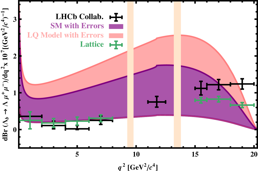
Figure 1: The dependence of the differential branching ratio on $q^{2}$ for the $\Lambda_{b}\rightarrow\Lambda\mu^{+}\mu^{-}$ transition in the SM and LQ models. The experimental data are taken from the LHCb Collaboration Ref. LHCb . The lattice predictions are borrowed from Ref. Detmold:2016pkz .The vertical shaded bands indicate the charmonia veto regions.

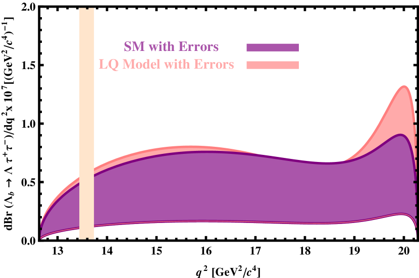
Figure 2: The dependence of the differential branching ratio on $q^{2}$ for the $\Lambda_{b}\rightarrow\Lambda\tau^{+}\tau^{-}$ transition in the SM and LQ models. The vertical shaded band indicates the charmonia veto region.

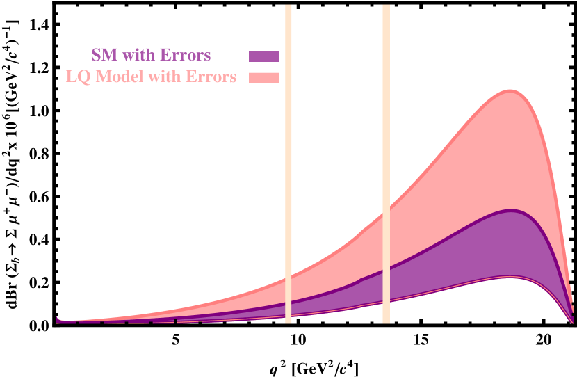
Figure 3: The dependence of the differential branching ratio on $q^{2}$ for the $\Sigma_{b}\rightarrow\Sigma\mu^{+}\mu^{-}$ transition in the SM and LQ models. The vertical shaded bands indicate the charmonia veto regions.

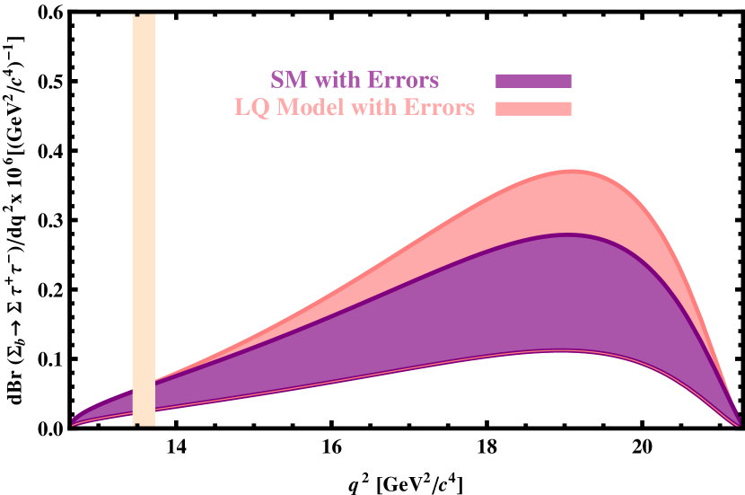
Figure 4: The dependence of the differential branching ratio on $q^{2}$ for the $\Sigma_{b}\rightarrow\Sigma\tau^{+}\tau^{-}$ transition in the SM and LQ models. The vertical shaded band indicates the charmonia veto region.

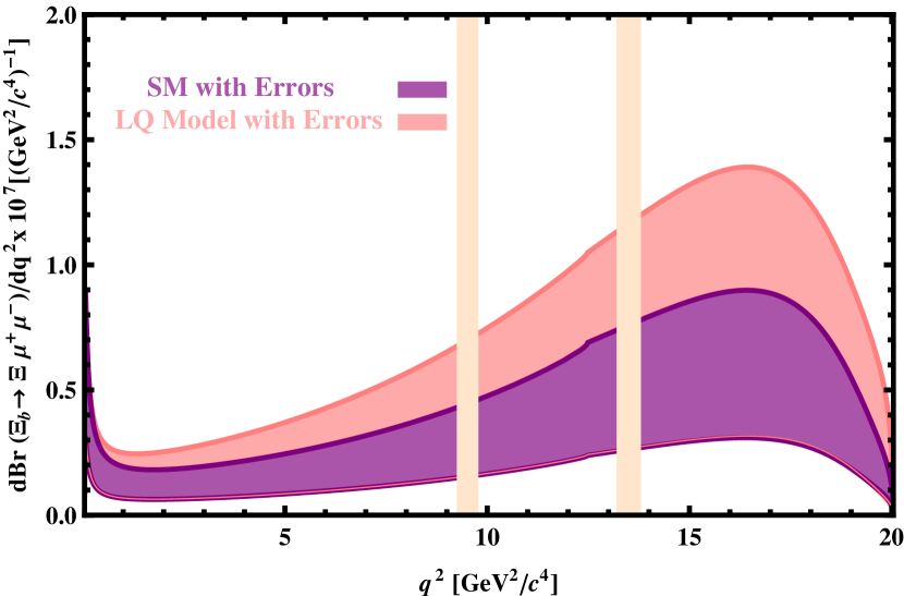
Figure 5: The dependence of the differential branching ratio on $q^{2}$ for the $\Xi_{b}\rightarrow\Xi\mu^{+}\mu^{-}$ transition in the SM and LQ models. The vertical shaded bands indicate the charmonia veto regions.

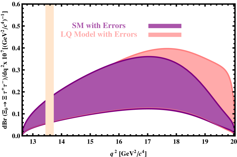
Figure 6: The dependence of the differential branching ratio on $q^{2}$ for the $\Xi_{b}\rightarrow\Xi\tau^{+}\tau^{-}$ transition in the SM and LQ models. The vertical shaded band indicates the charmonia veto region.

IV.3 The lepton forward-backward asymmetry

In this subsection, we present the results of the lepton forward-backward asymmetry (${\cal A}_{FB}$) which is one of useful observables to search for NP effects. This quantity is defined as

$${\cal A}_{FB}(\hat{s})=\frac{\displaystyle{\int_{0}^{1}\frac{d^{2}\Gamma}{d\hat{s}dz}}(z,\hat{s})\,dz-\displaystyle{\int_{-1}^{0}\frac{d^{2}\Gamma}{d\hat{s}dz}}(z,\hat{s})\,dz}{\displaystyle{\int_{0}^{1}\frac{d^{2}\Gamma}{d\hat{s}dz}}(z,\hat{s})\,dz+\displaystyle{\int_{-1}^{0}\frac{d^{2}\Gamma}{d\hat{s}dz}}(z,\hat{s})\,dz}~{}.$$ (11)

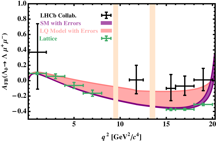
Figure 7: The dependence of the ${\cal A}_{FB}$ on $q^{2}$ for the $\Lambda_{b}\rightarrow\Lambda\mu^{+}\mu^{-}$ transition in the SM and LQ models. The experimental data are taken from the LHCb Collaboration Ref. LHCb . The lattice predictions are borrowed from Ref. Detmold:2016pkz . The vertical shaded bands indicate the charmonia veto regions.

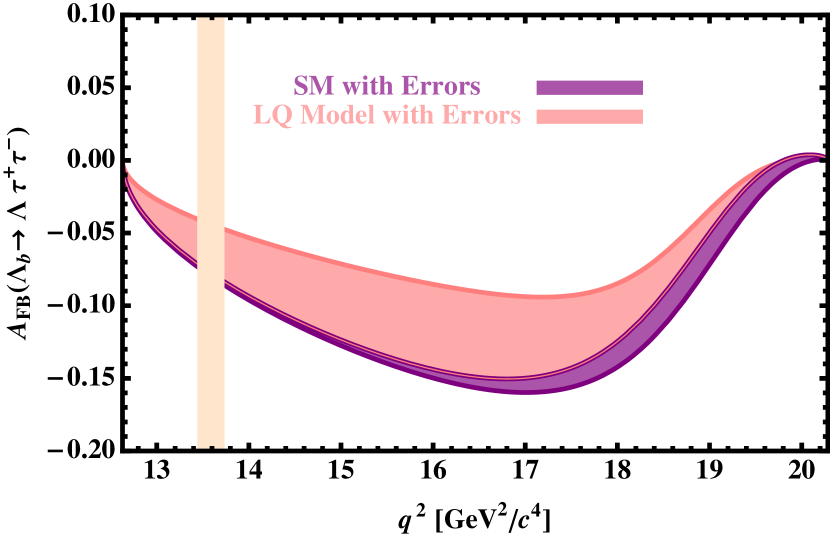
Figure 8: The dependence of the ${\cal A}_{FB}$ on $q^{2}$ for the $\Lambda_{b}\rightarrow\Lambda\tau^{+}\tau^{-}$ transition in the SM and LQ models. The vertical shaded band indicates the charmonia veto region.

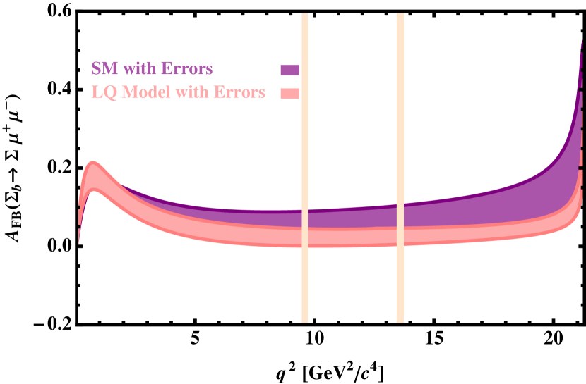
Figure 9: The dependence of the ${\cal A}_{FB}$ on $q^{2}$ for the $\Sigma_{b}\rightarrow\Sigma\mu^{+}\mu^{-}$ transition in the SM and LQ models. The vertical shaded bands indicate the charmonia veto regions.

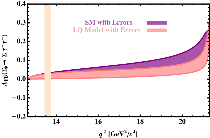
Figure 10: The dependence of the ${\cal A}_{FB}$ on $q^{2}$ for the $\Sigma_{b}\rightarrow\Sigma\tau^{+}\tau^{-}$ transition in the SM and LQ models. The vertical shaded band indicates the charmonia veto region.

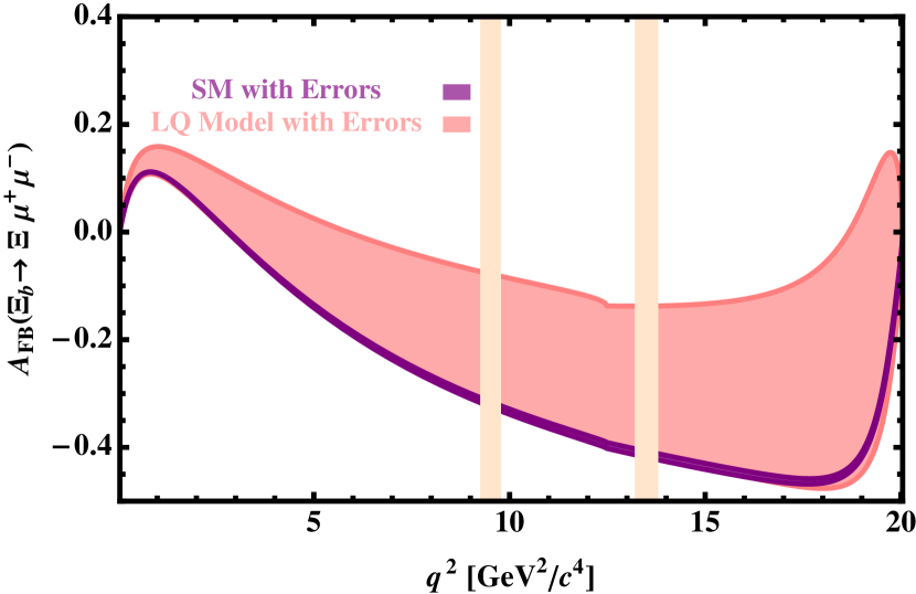
Figure 11: The dependence of the ${\cal A}_{FB}$ on $q^{2}$ for the $\Xi_{b}\rightarrow\Xi\mu^{+}\mu^{-}$ transition in the SM and LQ models. The vertical shaded bands indicate the charmonia veto regions.

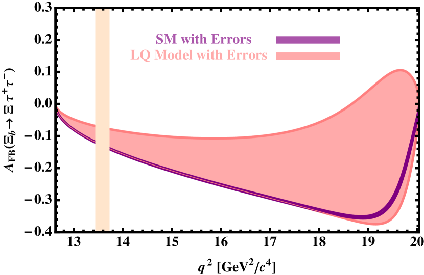
Figure 12: The dependence of the ${\cal A}_{FB}$ on $q^{2}$ for the $\Xi_{b}\rightarrow\Xi\tau^{+}\tau^{-}$ transition in the SM and LQ models. The vertical shaded band indicates the charmonia veto region.

In order to see how predictions of LQ scenario deviate from those of the SM, we plot the dependence of the lepton forward-backward asymmetry on $q^{2}$ for the channels under discussion in Figures 7-12. In figure 7, we also present the measured values of the leptonic forward backward-asymmetries by the LHCb Collaboration LHCb as well as the lattice QCD predictions Detmold:2016pkz in the $\Lambda_{b}\rightarrow\Lambda\mu^{+}\mu^{-}$ decay channel. From these figures, we read that

• in all decay channels the LQ model predictions demonstrate considerable discrepancies from the SM predictions.

• The SM band on the lepton forward-backward asymmetry in $\Lambda_{b}\rightarrow\Lambda\mu^{+}\mu^{-}$ channel coincides with the existing lattice QCD predictions borrowed from Ref. Detmold:2016pkz .

• Ignoring from the small intersection of the SM narrow bands with errors of the experimental data at very low and high values of $q^{2}$, the LQ model, against the SM, can describe all data available in $\Lambda_{b}\rightarrow\Lambda\mu^{+}\mu^{-}$ channel. The lattice QCD predictions in this channel also show sizable differences with the experimental data.

V Conclusion

In the present work, we have performed a comprehensive analysis of the semileptonic $\Lambda_{b}\rightarrow\Lambda\ell^{+}\ell^{-}$, $\Sigma_{b}\rightarrow\Sigma\ell^{+}\ell^{-}$ and $\Xi_{b}\rightarrow\Xi\ell^{+}\ell^{-}$ rare processes in the SM as well as the scalar leptoquark model. Using the parametrization of the matrix elements in terms of form factors calculated via light cone QCD sum rules in the full theory, we calculated the differential decay width and numerically analyzed the differential branching fraction and the lepton forward-backward asymmetry in terms of $q^{2}$ in different heavy baryonic decay channels for both the $\mu$ and $\tau$ leptons in both scenarios. We compared the predictions of the LQ model on the considered physical observables with those of the SM and the existing lattice QCD predictions as well as experimental data in $\Lambda_{b}\rightarrow\Lambda\mu^{+}\mu^{-}$ channel. We observed that the predictions of the LQ model in all channels show considerable discrepancies with those of the SM on both the differential decay width and lepton forward-backward asymmetry. The SM results for both the observables considered in the present study are consistent with the existing predictions of lattice QCD. Except the interval $18$ GeV${}^{2}/$c⁴ $\leq q^{2}\leq 20$ GeV${}^{2}/$c⁴, the SM band describes the existing experimental data on the differential branching ratio in $\Lambda_{b}\rightarrow\Lambda\mu^{+}\mu^{-}$ transition. The datum in $18$ GeV${}^{2}/$c⁴ $\leq q^{2}\leq 20$ GeV${}^{2}/$c⁴ coincides with the LQ model prediction.

In the case of lepton forward-backward asymmetry, the SM, overall, can not describe the experimental data existing in $\Lambda_{b}\rightarrow\Lambda\mu^{+}\mu^{-}$ channel, while the LQ model band coincides with the experimental data.

More experimental data in $\Lambda_{b}\rightarrow\Lambda\tau^{+}\tau^{-}$ as well as $\Sigma_{b}\rightarrow\Sigma\ell^{+}\ell^{-}$ and $\Xi_{b}\rightarrow\Xi\ell^{+}\ell^{-}$ with both leptons are needed to compare with the theoretical predictions. We hope, with the RUN II data, it will be possible to measure different physical quantities related to such FCNC transitions at LHCb in near future. Comparison of the future experimental data with the theoretical predictions on different physical quantities in various decay channels can help us better explain some anomalies between the SM predictions and the experimental data. Any sizable discrepancy between the theoretical predictions on physical observables with the experimental data can be considered as an indication of new physics effects and may help us in the course of searching for the new particles like leptoquarks.

Note Added: When preparing this work we noticed that a part of our work, namely the $\Lambda_{b}\rightarrow\Lambda\ell^{+}\ell^{-}$ channel has been investigated in Sahoo:2016nvx ; Wang:2016dne within the same framework. In these studies the authors use the form factors, as the main inputs, calculated in heavy quark effective theory while we use the form factors calculated via light cone QCD sum rules in full theory.

CONFLICT OF INTEREST

The authors declare that there is no conflict of interest regarding the publication of this paper.

*

Appendix A A

The Wilson coefficient $C_{7}^{eff}$ in leading logarithm approximation in the SM is written by Buras:1993xp ; Misiak ; Buras:1994dj ; Buras:1998raa

$$C_{7}^{eff}(\mu_{b}) = \eta^{\frac{16}{23}}C_{7}(\mu_{W})$$

$$+ \frac{8}{3}\left(\eta^{\frac{14}{23}}-\eta^{\frac{16}{23}}\right)C_{8}(\mu_{W})$$

$$+ C_{2}(\mu_{W})\sum_{i=1}^{8}h_{i}\eta^{a_{i}}~{},$$

where

$$C_{7}(\mu_{W}) = -\frac{1}{2}D^{\prime}_{0}(x_{t})~{},$$

$$C_{8}(\mu_{W}) = -\frac{1}{2}E^{\prime}_{0}(x_{t})~{},$$

$$C_{2}(\mu_{W}) = 1~{}.$$ (A.13)

The functions $D^{\prime}_{0}(x_{t})$ and $E^{\prime}_{0}(x_{t})$ with $x_{t}=\frac{m_{t}^{2}}{m_{W}^{2}}$ are given as

$$D^{\prime}_{0}(x_{t}) = -\frac{(8x_{t}^{3}+5x_{t}^{2}-7x_{t})}{12(1-x_{t})^{3}}$$

$$+ \frac{x_{t}^{2}(2-3x_{t})}{2(1-x_{t})^{4}}\ln x_{t}~{},$$

$$E^{\prime}_{0}(x_{t}) = -\frac{x_{t}(x_{t}^{2}-5x_{t}-2)}{4(1-x_{t})^{3}}$$ (A.15)

$$+ \frac{3x_{t}^{2}}{2(1-x_{t})^{4}}\ln x_{t}~{}.$$

The parameter $\eta$ in Eq.(A) is defined as

$$\eta\!\!\! = \!\!\!\frac{\alpha_{s}(\mu_{W})}{\alpha_{s}(\mu_{b})}~{},$$ (A.16)

with

$$\alpha_{s}(x)=\frac{\alpha_{s}(m_{Z})}{1-\beta_{0}\frac{\alpha_{s}(m_{Z})}{2\pi}\ln(\frac{m_{Z}}{x})}~{},$$ (A.17)

where $\alpha_{s}(m_{Z})=0.118$ and $\beta_{0}=\frac{23}{3}$. The coefficients $h_{i}$ and $a_{i}$ in Eq.(A) are also written by Misiak ; Buras:1994dj

$$\frac{}{}\begin{array}[]{rrrrrrrrrl}h_{i}&=&(\!\!&2.2996,&-1.0880,&-\frac{3}{7},&-\frac{1}{14},&\\ &-&0.6494,&-0.0380,&-0.0186,&-0.0057&\!\!)\vspace{0.1cm},\end{array}$$

$$\frac{}{}\begin{array}[]{rrrrrrrrrl}a_{i}&=&(\!\!&\frac{14}{23},&\frac{16}{23},&\frac{6}{23},&-\frac{12}{23},&\\ &&0.4086,&-0.4230,&-0.8994,&0.1456&\!\!).\end{array}$$ (A.18)

The Wilson coefficient $C_{9}^{eff}$ in SM is given by Misiak ; Buras:1994dj

$$C_{9}^{eff}(\hat{s}^{\prime}) = C_{9}^{NDR}\eta(\hat{s}^{\prime})$$ (A.19)

$$+ h(z,\hat{s}^{\prime})\left(3C_{1}+C_{2}+3C_{3}+C_{4}+3C_{5}+C_{6}\right)$$

$$- \frac{1}{2}h(1,\hat{s}^{\prime})\left(4C_{3}+4C_{4}+3C_{5}+C_{6}\right)$$

$$- \frac{1}{2}h(0,\hat{s}^{\prime})\left(C_{3}+3C_{4}\right)$$

$$+ \frac{2}{9}\left(3C_{3}+C_{4}+3C_{5}+C_{6}\right),$$

where $\hat{s}^{\prime}=\frac{q^{2}}{m_{b}^{2}}$ with $4m_{l}^{2}\leq q^{2}\leq(m_{{\cal B}_{Q}}-m_{\cal B})^{2}$. The $C_{9}^{NDR}$ in the naive dimensional regularization (NDR) scheme is written as

$$C_{9}^{NDR} = P_{0}^{NDR}+\frac{Y}{\sin^{2}\theta_{W}}$$ (A.20)

$$- 4Z+P_{E}E,$$

where $P_{0}^{NDR}=2.60\pm 0.25$, $\sin^{2}\theta_{W}=0.23$, $Y=0.98$ and $Z=0.679$ Misiak ; Buras:1994dj ; Buras:1998raa . The last term in Eq.(A.20) is ignored due to the negligible value of $P_{E}$. In Eq.(A.19), the $\eta(\hat{s}^{\prime})$ is given as

$$\eta(\hat{s}^{\prime}) = 1+\frac{\alpha_{s}(\mu_{b})}{\pi}\omega(\hat{s}^{\prime}),$$ (A.21)

with

$$\omega(\hat{s}^{\prime}) = -\frac{2}{9}\pi^{2}-\frac{4}{3}\mbox{Li}_{2}(\hat{s}^{\prime})-\frac{2}{3}\ln\hat{s}^{\prime}\ln(1-\hat{s}^{\prime})$$ (A.22)

$$- \frac{5+4\hat{s}^{\prime}}{3(1+2\hat{s}^{\prime})}\ln(1-\hat{s}^{\prime})$$

$$- \frac{2\hat{s}^{\prime}(1+\hat{s}^{\prime})(1-2\hat{s}^{\prime})}{3(1-\hat{s}^{\prime})^{2}(1+2\hat{s}^{\prime})}\ln\hat{s}^{\prime}$$

$$+ \frac{5+9\hat{s}^{\prime}-6\hat{s}^{\prime 2}}{6(1-\hat{s}^{\prime})(1+2\hat{s}^{\prime})}.$$

The function $h(y,\hat{s}^{\prime})$ is written as

$$h(y,\hat{s}^{\prime}) = -\frac{8}{9}\ln\frac{m_{b}}{\mu_{b}}-\frac{8}{9}\ln y+\frac{8}{27}+\frac{4}{9}x$$ (A.24)

$$-\frac{2}{9}(2+x)|1-x|^{1/2}$$

$$\left\{\begin{array}[]{ll}\left(\ln\left|\frac{\sqrt{1-x}+1}{\sqrt{1-x}-1}\right|-i\pi\right),&\mbox{for }x\equiv\frac{4z^{2}}{\hat{s}^{\prime}}<1\\ 2\arctan\frac{1}{\sqrt{x-1}},&\mbox{for }x\equiv\frac{4z^{2}}{\hat{s}^{\prime}}>1,\end{array}\right.$$

where $y=1$ or $y=z=\frac{m_{c}}{m_{b}}$ and

$$h(0,\hat{s}^{\prime}) = \frac{8}{27}-\frac{8}{9}\ln\frac{m_{b}}{\mu_{b}}-\frac{4}{9}\ln\hat{s}^{\prime}+\frac{4}{9}i\pi.$$ (A.26)

The coefficients $C_{j}$ (j=1,…6) at $\mu_{b}=5~{}GeV$ scale are also written as Buras:1998raa

$$C_{j}=\sum_{i=1}^{8}k_{ji}\eta^{a_{i}}\qquad(j=1,...6)\vspace{0.2cm},$$ (A.27)

where the $k_{ji}$ are given as

$$\frac{}{}\begin{array}[]{rrrrrrrrrl}k_{1i}&=&(\!\!&0,&0,&\frac{1}{2},&-\frac{1}{2},&\\ &&0,&0,&0,&0&\!\!),\vspace{0.1cm}\\ k_{2i}&=&(\!\!&0,&0,&\frac{1}{2},&\frac{1}{2},&\\ &&0,&0,&0,&0&\!\!),\vspace{0.1cm}\\ k_{3i}&=&(\!\!&0,&0,&-\frac{1}{14},&\frac{1}{6},&\\ &&0.0510,&-0.1403,&-0.0113,&0.0054&\!\!),\vspace{0.1cm}\\ k_{4i}&=&(\!\!&0,&0,&-\frac{1}{14},&-\frac{1}{6},&\\ &&0.0984,&0.1214,&0.0156,&0.0026&\!\!),\vspace{0.1cm}\\ k_{5i}&=&(\!\!&0,&0,&0,&0,&\\ &&-0.0397,&0.0117,&-0.0025,&0.0304&\!\!),\vspace{0.1cm}\\ k_{6i}&=&(\!\!&0,&0,&0,&0,&\\ &&0.0335,&0.0239,&-0.0462,&-0.0112&\!\!).\vspace{0.1cm}\\ \end{array}$$

Considering the resonances from $J/\psi$ family, we divide the allowed physical region into the following three regions in the case of the electron and muon as final leptons:

$$Region~{}I 4m_{l}^{2}\leq q^{2}\leq(m_{J/\psi(1s)}-0.02)^{2},$$ ;

$$Region~{}II (m_{J/\psi(1s)}+0.02)^{2}\leq q^{2}\leq(m_{\psi(2s)}-0.02)^{2},$$ ;

$$Region~{}III (m_{\psi(2s)}+0.02)^{2}\leq q^{2}\leq(m_{{\cal B}_{Q}}-m_{{\cal B}})^{2}.$$ ;

In the case of $\tau$, we have the following two regions:

$$Region~{}I 4m_{\tau}^{2}\leq q^{2}\leq(m_{\psi(2s)}-0.02)^{2},$$ ;

$$Region~{}II (m_{\psi(2s)}+0.02)^{2}\leq q^{2}\leq(m_{{\cal B}_{Q}}-m_{{\cal B}})^{2}.$$ ;

The Wilson coefficient $C_{10}$ in the SM is given as:

$$C_{10}=-\frac{Y}{\sin^{2}\theta_{W}}~{}.$$ (A.28)

Appendix B B

The calligraphic coefficients used in the transition amplitudes of the considered processes are find as

$${\cal A}_{1} = f_{1}C_{9}^{eff+}-g_{1}C_{9}^{eff-}$$

$$- 2m_{b}{1\over q^{2}}\Big{[}f_{1}^{T}C_{7}^{eff+}+g_{1}^{T}C_{7}^{eff-}\Big{]},~{}$$

$${\cal A}_{2} = {\cal A}_{1}(1\rightarrow 2),~{}$$

$${\cal A}_{3} = {\cal A}_{1}\left(1\rightarrow 3\right)~{},$$

$${\cal B}_{1} = f_{1}C_{9}^{eff+}+g_{1}C_{9}^{eff-}$$

$$- 2m_{b}{1\over q^{2}}\Big{[}f_{1}^{T}C_{7}^{eff+}-g_{1}^{T}C_{7}^{eff-}\Big{]},~{}$$

$${\cal B}_{2} = {\cal B}_{1}\left(1\rightarrow 2\right),~{}$$

$${\cal B}_{3} = {\cal B}_{1}\left(1\rightarrow 3\right)~{},$$

$${\cal D}_{1} = f_{1}C_{10}^{+}-g_{1}C_{10}^{-},~{}$$

$${\cal D}_{2} = {\cal D}_{1}\left(1\rightarrow 2\right)~{},$$

$${\cal D}_{3} = {\cal D}_{1}\left(1\rightarrow 3\right)~{},$$

$${\cal E}_{1} = f_{1}C_{10}^{+}+g_{1}C_{10}^{-}~{},$$

$${\cal E}_{2} = {\cal E}_{1}\left(1\rightarrow 2\right)~{},$$

$${\cal E}_{3} = {\cal E}_{1}\left(1\rightarrow 3\right)~{},$$

with

$$C_{9}^{eff+} = C_{9}^{eff}+C^{\prime~{}eff}_{9}~{},$$

$$C_{9}^{eff-} = C_{9}^{eff}-C^{\prime~{}eff}_{9}~{},$$

$$C_{7}^{eff+} = C_{7}^{eff}+C^{\prime~{}eff}_{7}~{},$$

$$C_{7}^{eff-} = C_{7}^{eff}-C^{\prime~{}eff}_{7}~{},$$

$$C_{10}^{+} = C_{10}+C^{\prime}_{10}~{},$$

$$C_{10}^{-} = C_{10}-C^{\prime}_{10}~{}.$$

The functions ${\cal T}_{0}^{tot}(\hat{s})$, ${\cal T}_{1}^{tot}(\hat{s})$ and ${\cal T}_{2}^{tot}(\hat{s})$ in the differential decay width are given as

$${\cal T}_{0}^{tot}(\hat{s})\!\!\! = \!\!\!32m_{\ell}^{2}m_{{\cal B}_{Q}}^{4}\hat{s}(1+r-\hat{s})\Big{(}\left|{\cal D}_{3}\right|^{2}+\left|{\cal E}_{3}\right|^{2}\Big{)}$$

$$+ \!\!\!64m_{\ell}^{2}m_{{\cal B}_{Q}}^{3}(1-r-\hat{s})\,\mbox{\rm Re}\Big{[}{\cal D}_{1}^{\ast}{\cal E}_{3}+{\cal D}_{3}{\cal E}_{1}^{\ast}\Big{]}$$

$$+ \!\!\!64m_{{\cal B}_{Q}}^{2}\sqrt{r}(6m_{\ell}^{2}-m_{{\cal B}_{Q}}^{2}\hat{s}){\rm Re}\Big{[}{\cal D}_{1}^{\ast}{\cal E}_{1}\Big{]}$$

$$+ \!\!\!64m_{\ell}^{2}m_{{\cal B}_{Q}}^{3}\sqrt{r}\Bigg{\{}2m_{{\cal B}_{Q}}\hat{s}{\rm Re}\Big{[}{\cal D}_{3}^{\ast}{\cal E}_{3}\Big{]}+(1-r+\hat{s}){\rm Re}\Big{[}{\cal D}_{1}^{\ast}{\cal D}_{3}+{\cal E}_{1}^{\ast}{\cal E}_{3}\Big{]}\Bigg{\}}$$

$$+ \!\!\!32m_{{\cal B}_{Q}}^{2}(2m_{\ell}^{2}+m_{{\cal B}_{Q}}^{2}\hat{s})\Bigg{\{}(1-r+\hat{s})m_{{\cal B}_{Q}}\sqrt{r}\,\mbox{\rm Re}\Big{[}{\cal A}_{1}^{\ast}{\cal A}_{2}+{\cal B}_{1}^{\ast}{\cal B}_{2}\Big{]}$$

$$- \!\!\!m_{{\cal B}_{Q}}(1-r-\hat{s})\,\mbox{\rm Re}\Big{[}{\cal A}_{1}^{\ast}{\cal B}_{2}+{\cal A}_{2}^{\ast}{\cal B}_{1}\Big{]}-2\sqrt{r}\Big{(}\mbox{\rm Re}\Big{[}{\cal A}_{1}^{\ast}{\cal B}_{1}\Big{]}+m_{{\cal B}_{Q}}^{2}\hat{s}\,\mbox{\rm Re}\Big{[}{\cal A}_{2}^{\ast}{\cal B}_{2}\Big{]}\Big{)}\Bigg{\}}$$

$$+ \!\!\!8m_{{\cal B}_{Q}}^{2}\Bigg{\{}4m_{\ell}^{2}(1+r-\hat{s})+m_{{\cal B}_{Q}}^{2}\Big{[}(1-r)^{2}-\hat{s}^{2}\Big{]}\Bigg{\}}\Big{(}\left|{\cal A}_{1}\right|^{2}+\left|{\cal B}_{1}\right|^{2}\Big{)}$$

$$+ \!\!\!8m_{{\cal B}_{Q}}^{4}\Bigg{\{}4m_{\ell}^{2}\Big{[}\lambda+(1+r-\hat{s})\hat{s}\Big{]}+m_{{\cal B}_{Q}}^{2}\hat{s}\Big{[}(1-r)^{2}-\hat{s}^{2}\Big{]}\Bigg{\}}\Big{(}\left|{\cal A}_{2}\right|^{2}+\left|{\cal B}_{2}\right|^{2}\Big{)}$$

$$- \!\!\!8m_{{\cal B}_{Q}}^{2}\Bigg{\{}4m_{\ell}^{2}(1+r-\hat{s})-m_{{\cal B}_{Q}}^{2}\Big{[}(1-r)^{2}-\hat{s}^{2}\Big{]}\Bigg{\}}\Big{(}\left|{\cal D}_{1}\right|^{2}+\left|{\cal E}_{1}\right|^{2}\Big{)}$$

$$+ \!\!\!8m_{{\cal B}_{Q}}^{5}\hat{s}v^{2}\Bigg{\{}-8m_{{\cal B}_{Q}}\hat{s}\sqrt{r}\,\mbox{\rm Re}\Big{[}{\cal D}_{2}^{\ast}{\cal E}_{2}\Big{]}+4(1-r+\hat{s})\sqrt{r}\,\mbox{\rm Re}\Big{[}{\cal D}_{1}^{\ast}{\cal D}_{2}+{\cal E}_{1}^{\ast}{\cal E}_{2}\Big{]}$$

$$- \!\!\!4(1-r-\hat{s})\,\mbox{\rm Re}\Big{[}{\cal D}_{1}^{\ast}{\cal E}_{2}+{\cal D}_{2}^{\ast}{\cal E}_{1}\Big{]}+m_{{\cal B}_{Q}}\Big{[}(1-r)^{2}-\hat{s}^{2}\Big{]}\Big{(}\left|{\cal D}_{2}\right|^{2}+\left|{\cal E}_{2}\right|^{2}\Big{)}\Bigg{\}},$$

$${\cal T}_{1}^{tot}(\hat{s}) = -16m_{{\cal B}_{Q}}^{4}\hat{s}v\sqrt{\lambda}\Bigg{\{}2Re\Big{(}{\cal A}_{1}^{*}{\cal D}_{1}\Big{)}-2Re\Big{(}{\cal B}_{1}^{*}{\cal E}_{1}\Big{)}$$

$$+ 2m_{{\cal B}_{Q}}Re\Big{(}{\cal B}_{1}^{*}{\cal D}_{2}-{\cal B}_{2}^{*}{\cal D}_{1}+{\cal A}_{2}^{*}{\cal E}_{1}-{\cal A}_{1}^{*}{\cal E}_{2}\Big{)}\Bigg{\}}$$

$$+ 32m_{{\cal B}_{Q}}^{5}\hat{s}~{}v\sqrt{\lambda}\Bigg{\{}m_{{\cal B}_{Q}}(1-r)Re\Big{(}{\cal A}_{2}^{*}{\cal D}_{2}-{\cal B}_{2}^{*}{\cal E}_{2}\Big{)}$$

$$+ \sqrt{r}Re\Big{(}{\cal A}_{2}^{*}{\cal D}_{1}+{\cal A}_{1}^{*}{\cal D}_{2}-{\cal B}_{2}^{*}{\cal E}_{1}-{\cal B}_{1}^{*}{\cal E}_{2}\Big{)}\Bigg{\}},$$

and

$${\cal T}_{2}^{tot}(\hat{s})\!\!\! = \!\!\!-8m_{{\cal B}_{Q}}^{4}v^{2}\lambda\Big{(}\left|{\cal A}_{1}\right|^{2}+\left|{\cal B}_{1}\right|^{2}+\left|{\cal D}_{1}\right|^{2}+\left|{\cal E}_{1}\right|^{2}\Big{)}$$

$$+ \!\!\!8m_{{\cal B}_{Q}}^{6}\hat{s}v^{2}\lambda\Big{(}\left|{\cal A}_{2}\right|^{2}+\left|{\cal B}_{2}\right|^{2}+\left|{\cal D}_{2}\right|^{2}+\left|{\cal E}_{2}\right|^{2}\Big{)}~{}.$$

References

• (1) T. Aaltonen et al. [CDF Collaboration], “Observation of the Baryonic Flavor-Changing Neutral Current Decay $\Lambda_{b}\to\Lambda\mu^{+}\mu^{-}$,” Phys. Rev. Lett.  107, 201802 (2011) [arXiv:1107.3753 [hep-ex]].
• (2) The LHCb Collaboration, “Differential branching fraction and angular analysis of $\Lambda^{0}_{b}\rightarrow\Lambda\mu^{+}\mu^{-}$ decays”, JHEP 1506 115 (2015) [arXiv:1503.07138 [hep-ex]].
• (3) T. M. Aliev, K. Azizi and M. Savci, “Analysis of the $\Lambda_{b}\rightarrow\Lambda\ell^{+}\ell^{-}$ decay in QCD,” Phys. Rev. D 81, 056006 (2010) [arXiv:1001.0227 [hep-ph]].
• (4) K. Azizi, M. Bayar, A. Ozpineci, Y. Sarac and H. Sundu, “Semileptonic transition of $\Sigma_{b}$ to $\Sigma$ in Light Cone QCD Sum Rules,” Phys. Rev. D 85, 016002 (2012) [arXiv:1112.5147 [hep-ph]].
• (5) K. Azizi, Y. Sarac and H. Sundu, “Light cone QCD sum rules study of the semileptonic heavy $\Xi_{Q}$ and $\Xi^{\prime}_{Q}$ transitions to $\Xi$ and $\Sigma$ baryons,” Eur. Phys. J. A 48, 2 (2012) [arXiv:1107.5925 [hep-ph]].
• (6) K. Azizi, S. Kartal, N. Katirci, A. T. Olgun and Z. Tavukoglu, “Constraint on compactification scale via recently observed baryonic $\Lambda_{b}\rightarrow\Lambda\ell^{+}\ell^{-}$ channel and analysis of the $\Sigma_{b}\rightarrow\Sigma\ell^{+}\ell^{-}$ transition in SM and UED scenario,” JHEP 1205, 024 (2012) [arXiv:1203.4356 [hep-ph]].
• (7) K. Azizi, S. Kartal, A. T. Olgun and Z. Tavukoglu, “Analysis of the semileptonic $\Lambda_{b}\rightarrow\Lambda\ell^{+}\ell^{-}$ transition in the topcolor-assisted technicolor model,” Phys. Rev. D 88, no. 7, 075007 (2013) [arXiv:1307.3101 [hep-ph]].
• (8) B. Dumont, K. Nishiwaki and R. Watanabe, “LHC constraints and prospects for $S_{1}$ scalar leptoquark explaining the $\bar{B}\to D^{(*)}\tau\bar{\nu}$ anomaly,” arXiv:1603.05248 [hep-ph].
• (9) K.  A.  Olive et al. (Particle Data Group), Chin. Phys. C 38, 090001 (2014).
• (10) I. Doršner, S. Fajfer, A. Greljo, J. F. Kamenik and N. Košnik, “Physics of leptoquarks in precision experiments and at particle colliders,” arXiv:1603.04993 [hep-ph].
• (11) S. Davidson, D. C. Bailey and B. A. Campbell, “Model independent constraints on leptoquarks from rare processes,” Z. Phys. C 61, 613 (1994) [hep-ph/9309310].
• (12) J. L. Hewett and T. G. Rizzo, “Much ado about leptoquarks: A Comprehensive analysis,” Phys. Rev. D 56, 5709 (1997) [hep-ph/9703337].
• (13) O. U. Shanker, “Flavor Violation, Scalar Particles and Leptoquarks,” Nucl. Phys. B 206, 253 (1982).
• (14) S. Fajfer and N. Kosnik, “Leptoquarks in FCNC charm decays,” Phys. Rev. D 79, 017502 (2009) [arXiv:0810.4858 [hep-ph]].
• (15) J. P. Saha, B. Misra and A. Kundu, “Constraining Scalar Leptoquarks from the K and B Sectors,” Phys. Rev. D 81, 095011 (2010) [arXiv:1003.1384 [hep-ph]].
• (16) S. Davidson and P. Verdier, “Leptoquarks decaying to a top quark and a charged lepton at hadron colliders,” Phys. Rev. D 83, 115016 (2011) [arXiv:1102.4562 [hep-ph]].
• (17) N. Kosnik, “Model independent constraints on leptoquarks from $b\to s\ell^{+}\ell^{-}$ processes,” Phys. Rev. D 86, 055004 (2012) [arXiv:1206.2970 [hep-ph]].
• (18) J. M. Arnold, B. Fornal and M. B. Wise, “Phenomenology of scalar leptoquarks,” Phys. Rev. D 88, 035009 (2013) [arXiv:1304.6119 [hep-ph]].
• (19) Y. Sakaki, M. Tanaka, A. Tayduganov and R. Watanabe, “Testing leptoquark models in $\bar{B}\to D^{(*)}\tau\bar{\nu}$,” Phys. Rev. D 88, no. 9, 094012 (2013) [arXiv:1309.0301 [hep-ph]].
• (20) R. Mohanta, “Effect of scalar leptoquarks on the rare decays of $B_{s}$ meson,” Phys. Rev. D 89, no. 1, 014020 (2014) [arXiv:1310.0713 [hep-ph]].
• (21) B. Allanach, A. Alves, F. S. Queiroz, K. Sinha and A. Strumia, “Interpreting the CMS $\ell^{+}\ell^{-}jjE\!\!\!\!/_{\rm T}$ Excess with a Leptoquark Model,” Phys. Rev. D 92, no. 5, 055023 (2015) [arXiv:1501.03494 [hep-ph]].
• (22) S. Sahoo and R. Mohanta, “Scalar leptoquarks and the rare $B$ meson decays,” Phys. Rev. D 91, no. 9, 094019 (2015) [arXiv:1501.05193 [hep-ph]].
• (23) S. Sahoo and R. Mohanta, “Study of the rare semileptonic decays $B_{d}^{0}\to K^{*}l^{+}l^{-}$ in scalar leptoquark model,” Phys. Rev. D 93, no. 3, 034018 (2016) [arXiv:1507.02070 [hep-ph]].
• (24) S. Sahoo and R. Mohanta, “Leptoquark effects on $b\;\to\;s{\boldsymbol{\nu}}\bar{{\boldsymbol{\nu}}}$ and $B\;\to\;{{Kl}}^{+}{l}^{-}$ decay processes,” New J. Phys.  18, no. 1, 013032 (2016) [arXiv:1509.06248 [hep-ph]].
• (25) S. Sahoo and R. Mohanta, “Lepton flavor violating B meson decays via a scalar leptoquark,” Phys. Rev. D 93, no. 11, 114001 (2016) [arXiv:1512.04657 [hep-ph]].
• (26) G. Kumar, “Constraints on Scalar Leptoquark from Kaon Sector,” arXiv:1603.00346 [hep-ph].
• (27) I. Dorsner, S. Fajfer, J. F. Kamenik and N. Kosnik, “Can scalar leptoquarks explain the $f_{D_{s}}$ puzzle?,” Phys. Lett. B 682, 67 (2009) [arXiv:0906.5585 [hep-ph]].
• (28) I. Dorsner, J. Drobnak, S. Fajfer, J. F. Kamenik and N. Kosnik, “Limits on scalar leptoquark interactions and consequences for GUTs,” JHEP 1111, 002 (2011) [arXiv:1107.5393 [hep-ph]].
• (29) D. Becirevic, N. Kosnik, O. Sumensari and R. Zukanovich Funchal, “Palatable Leptoquark Scenarios for Lepton Flavor Violation in Exclusive $b\to s\ell_{1}\ell_{2}$ modes,” JHEP 1611, 035 (2016) [arXiv:1608.07583 [hep-ph]].
• (30) D. Becirevic, S. Fajfer, N. Kosnik and O. Sumensari, “Leptoquark model to explain the $B$-physics anomalies, $R_{K}$ and $R_{D}$,” Phys. Rev. D 94, no. 11, 115021 (2016) [ arXiv:1608.08501 [hep-ph]].
• (31) G. Buchalla, A. J. Buras and M. E. Lautenbacher, “Weak decays beyond leading logarithms,” Rev. Mod. Phys.  68, 1125 (1996) [hep-ph/9512380].
• (32) W. Altmannshofer, P. Ball, A. Bharucha, A. J. Buras, D. M. Straub and M. Wick, “Symmetries and Asymmetries of $B\to K^{*}\mu^{+}\mu^{-}$ Decays in the Standard Model and Beyond,” JHEP 0901, 019 (2009) [arXiv:0811.1214 [hep-ph]].
• (33) S. Sahoo and R. Mohanta, “Effects of scalar leptoquark on semileptonic $\Lambda_{b}$ decays,” New J. Phys.  18, no. 9, 093051 (2016) [ arXiv:1607.04449 [hep-ph]].
• (34) T. Feldmann and M. W. Y. Yip, “Form Factors for $\Lambda_{b}\to\Lambda$ Transitions in SCET,” Phys. Rev. D 85, 014035 (2012) Erratum: [Phys. Rev. D 86, 079901 (2012)] [arXiv:1111.1844 [hep-ph]].
• (35) P. Böer, T. Feldmann and D. van Dyk, “Angular Analysis of the Decay $\Lambda_{b}\to\Lambda(\to N\pi)\ell^{+}\ell^{-}$,” JHEP 1501, 155 (2015) [arXiv:1410.2115 [hep-ph]].
• (36) Y. M. Wang and Y. L. Shen, “Perturbative Corrections to $\Lambda_{b}\to\Lambda$ Form Factors from QCD Light-Cone Sum Rules,” JHEP 1602, 179 (2016) [arXiv:1511.09036 [hep-ph]].
• (37) W. Detmold and S. Meinel, “$\Lambda_{b}\to\Lambda\ell^{+}\ell^{-}$ form factors, differential branching fraction, and angular observables from lattice QCD with relativistic $b$ quarks,” Phys. Rev. D 93, no. 7, 074501 (2016) [arXiv:1602.01399 [hep-lat]].
• (38) S. Descotes-Genon, J. Matias and J. Virto, “Understanding the $B\to K^{*}\mu^{+}\mu^{-}$ Anomaly,” Phys. Rev. D 88, 074002 (2013) [arXiv:1307.5683 [hep-ph]].
• (39) T. Hurth, F. Mahmoudi and S. Neshatpour, “Global fits to $b\to s\ell\ell$ data and signs for lepton non-universality,” JHEP 1412, 053 (2014) [arXiv:1410.4545 [hep-ph]].
• (40) F. Beaujean, C. Bobeth and S. Jahn, “Constraints on tensor and scalar couplings from $B\rightarrow K\bar{\mu}\mu$ and $B_{s}\rightarrow\bar{\mu}\mu$,” Eur. Phys. J. C 75, no. 9, 456 (2015) [arXiv:1508.01526 [hep-ph]].
• (41) D. Du, A. X. El-Khadra, S. Gottlieb, A. S. Kronfeld, J. Laiho, E. Lunghi, R. S. Van de Water and R. Zhou, “Phenomenology of semileptonic B-meson decays with form factors from lattice QCD,” Phys. Rev. D 93, no. 3, 034005 (2016) [arXiv:1510.02349 [hep-ph]].
• (42) S. Descotes-Genon, L. Hofer, J. Matias and J. Virto, “Global analysis of $b\to s\ell\ell$ anomalies,” JHEP 1606, 092 (2016) [arXiv:1510.04239 [hep-ph]].
• (43) T. Hurth, F. Mahmoudi and S. Neshatpour, “On the anomalies in the latest LHCb data,” Nucl. Phys. B 909, 737 (2016) [arXiv:1603.00865 [hep-ph]].
• (44) S. Meinel and D. van Dyk, “Using $\Lambda_{b}\to\Lambda\mu^{+}\mu^{-}$ data within a Bayesian analysis of $|\Delta B|=|\Delta S|=1$ decays,” Phys. Rev. D 94, no. 1, 013007 (2016) [arXiv:1603.02974 [hep-ph]].
• (45) S. w. Wang and Y. d. Yang, “Analysis of $\Lambda_{b}\rightarrow$ $\Lambda\mu^{+}\mu^{-}$ decay in scalar leptoquark model,” Adv. High Energy Phys.  2016, 5796131 (2016) [arXiv:1608.03662 [hep-ph]].
• (46) A. J. Buras, M. Misiak, M. Munz and S. Pokorski, “Theoretical uncertainties and phenomenological aspects of $B\rightarrow X(s)$ gamma decay,” Nucl. Phys. B 424, 374 (1994) [hep-ph/9311345].
• (47) M. Misiak, “The $b\rightarrow se^{+}e^{-}$ and $b\rightarrow s\gamma$ decays with next-to-leading logarithmic QCD-corrections”, Nucl. Phys. B 393, 23 (1993); Erratum-ibid B 439, 161 (1995).
• (48) A. J. Buras and M. Munz, “Effective Hamiltonian for $B\rightarrow X(s)e^{+}e^{-}$ beyond leading logarithms in the NDR and HV schemes,” Phys. Rev. D 52, 186 (1995) [hep-ph/9501281].
• (49) A. J. Buras, “Weak Hamiltonian, CP violation and rare decays,” to appear in “Probing the Standard Model of Particle Interactions”, F. David and R. Gupta, eds, Elsevier Science B.V. [ hep-ph/9806471].