Algebraic and logical descriptions
of generalized trees

Abstract.

Quasi-trees generalize trees in that the unique “path” between two nodes may be infinite and have any countable order type. They are used to define the rank-width of a countable graph in such a way that it is equal to the least upper-bound of the rank-widths of its finite induced subgraphs. Join-trees are the corresponding directed trees. They are useful to define the modular decomposition of a countable graph. We also consider ordered join-trees, that generalize rooted trees equipped with a linear order on the set of sons of each node. We define algebras with finitely many operations that generate (via infinite terms) these generalized trees. We prove that the associated regular objects (those defined by regular terms) are exactly the ones that are the unique models of monadic second-order sentences. These results use and generalize a similar result by W. Thomas for countable linear orders.

Introduction

We define and study countable generalized trees, called quasi-trees, such that the unique “path” between two nodes may be infinite and have any order type, in particular that of rational numbers. Our motivation comes from the notion of rank-width, a complexity measure of finite graphs investigated first in [21] and [22]. Rank-width is based on graph decompositions formalized with finite undirected trees of maximal degree at most 3. In order to extend it to countable graphs in such a way that the compactness property holds, i.e., that the rank-width of a countable graph is the least upper bound of those of its finite induced subgraphs, we base decompositions on quasi-trees [11]. Quasi-trees arise as least upper bounds of increasing sequences of finite trees, $H_{1}\subseteq H_{2}\subseteq\dots\subseteq H_{n}\subseteq\dots,$ where $H_{i+1}$ is obtained from $H_{i}$ by the addition of a new node, either linked to an existing one by a new edge or inserted on an existing edge. If one inserts infinitely many nodes on an edge of some $H_{i}$, then, the least upper bound is not a tree but a quasi-tree.

Join-trees can be seen as directed quasi-trees. A join-tree is a partial order $(N,\leq)$ such that every two elements have a least upper bound (called their join) and each set $\{y\mid y\geq x\}$ is linearly ordered. The modular decomposition of a countable graph is based on an ordered join-tree [13].

Our objective is to obtain finitary descriptions (usable in algorithms) of generalized trees that are of the following three types: join-trees, ordered join-trees and quasi-trees. For this purpose, we will define, for each type of generalized tree, an algebra based on finitely many operations such that the finite and infinite terms over these operations define all generalized trees of this type. The regular generalized trees are those defined by regular terms, i.e. that have finitely many different subterms, equivalently, that are the unique solutions of certain finite equation systems. We will prove that a generalized tree is regular if and only if it is monadic second-order definable, i.e., is the unique finite or countable model (up to isomorphism) of a monadic second-order sentence.

As a special case, we have linear orders. A countable linear order whose elements are labelled by letters from a finite alphabet is called an arrangement. The linear order of a regular arrangement is the left-right order of the leaves of the tree representing a regular term, equivalently, the lexicographic ordering of the words of a regular language. Regular arrangements were first defined and studied in [8] and [18], and their monadic second-order definability was proved in [23]. We will use the latter result for proving its extension to our generalized trees.

The study of regular linear orders has been continued by Bloom and Ésik in [1, 2]. They have also studied the algebraic linear orders, defined similarly from algebraic trees (infinite terms that are solutions of certain first-order equation systems, cf. [9]) or equivalently, as lexicographic orderings of the words of deterministic context-free languages [3, 4].

In Sections 1 and 2, we review definitions and basic results. In Section 3, we first study binary join-trees and then, we extend the definitions and results concerning them to all join-trees. In Section 4, we study ordered join-trees, and, in Section 5, we study quasi-trees. An introductory article on these results is [12].

1. Orders, trees and terms

All sets, trees and logical structures are finite or countably infinite. We denote by $X\uplus Y$ the union of sets $X$ and $Y$ if they are disjoint. Isomorphism of ordered sets, trees and other logical structures is denoted by $\simeq$. The restriction of a relation $R$ or a function $f$ defined on a set $V$ to a subset $W$ of $V$ is denoted by $R\upharpoonright W$ or $f\upharpoonright W$ respectively.

For partial orders $\leq,\preceq,\sqsubseteq$, …we denote respectively by $<,\prec,\sqsubset$, …the corresponding strict orders and $X<Y$ means that $x<y$ for every $x\in X$ and $y\in Y$.

Let $(V,\leq)$ be a partial order. The least upper bound of $x$ and $y$ is denoted by $x\sqcup y$ if it exists and is called their join. The notation $x\bot y$ means that $x$ and $y$ are incomparable. A line is a subset $Y$ of $V$ that is linearly ordered and satisfies the following convexity property: if $x,z\in Y$, $y\in V$ and $x\leq y\leq z$, then $y\in Y$. Particular notations for convex sets (not necessarly linearly ordered) are $[x,y]$ denoting $\{z\mid x\leq z\leq y\}$, $\mathopen{]}x,y]$ denoting $\{z\mid x<z\leq y\}$, $\mathopen{]}-\infty,x]$ denoting $\{y\mid y\leq x\}$ (even if $V$ is finite), $\mathopen{]}x,+\infty\mathclose{[}$ denoting $\{y\mid x<y\}$ etc. If $X\subseteq V$, then $\mathord{\downarrow}(X)$ is the union of the sets $\mathopen{]}-\infty,x]$ for $x$ in $X$.

The first infinite ordinal and the linear order $(\mathbb{N},\leq)$ are denoted by $\omega$.

Let $A$ be a finite set that is linearly ordered by $\leq$, and $A^{\ast}$ be the set of finite words over $A$; the empty word is $\varepsilon$. This set is linearly ordered by the lexicographic order $\leq_{lex}$ defined by $u\leq_{lex}v$ if and only if $v=uw$ or, $u=wax$ and $u=wby$ for some $w,x,y$ in $A^{\ast}$ and $a,b$ in $A$ such that $a<b$. Every finite or countable linear order is isomorphic to $(L,\leq_{lex})$ for some set $L\subseteq\{0,1\}^{\ast}$ that is prefix-free, which means that, if $u,uv\in L$ where $v\in\{0,1\}^{\ast},$ then $v=\varepsilon$ (Theorem 1.7 of [8]). The case where $L$ is regular has been studied in [1, 2, 8, 18, 23].

1.1. Trees

A tree is a possibly empty, finite or countable, undirected graph that is connected and has no cycles. Hence, it has neither loops nor parallel edges (it has no two edges with same ends). The set of nodes of a tree $T$ is $N_{T}$.

A rooted tree is a nonempty tree equipped with a distinguished node called its root. The level of a node $x$ is the number of edges of the path between it and the root and $Sons(x)$ denotes the set of its sons. We define on $N_{T}$ the partial order $\leq_{T}$ such that $x\leq_{T}y$ if and only if $y$ is on the unique path between $x$ and the root. The least upper bound of $x$ and $y$, denoted by $x\sqcup_{T}y,$ is their least common ancestor. We will specify a rooted tree $T$ by $(N_{T},\leq_{T})$ and we will omit the index $T$ when the considered tree is clear. For a node $x$ of $T$, the subtree issued from $x,$ denoted by $T/x,$ is defined as $(N_{T/x},\leq_{T}\upharpoonright N_{T/x})$ where $N_{T/x}:=\mathopen{]}-\infty,x]$.

A partial order $(N,\leq)$ is $(N_{T},\leq_{T})$ for some rooted tree $T$ if and only if it has a largest element $max$ and for each $x\in N$, the set $[x,max]$ is finite and linearly ordered. These conditions imply that any two nodes have a join.

An ordered tree is a rooted tree such that each set $Sons(x)$ is linearly ordered by an order $\sqsubseteq_{x}$.

1.2. Finite and infinite terms

Let $F$ be a finite set of operations, each $f$ in $F$ being given with an arity $\rho(f)$. We call $(F,\rho)$ a signature. The maximal arity of a symbol is denoted by $\rho(F)$. A term over $F$ is finite or infinite. We denote by $T^{\infty}(F)$ the set of all terms over $F$ and by $T(F)$ the set of finite ones. A typical example of an infinite term, easily describable linearly, is, with $f$ binary and $a$ and $b$ nullary, the term $t_{\infty}:=f(a,f(b,f(a,f(b,f(\dots))))))$ that is the unique solution in $T^{\infty}(F)$ of the equation $t=f(a,f(b,t))$.

Positions in terms are designated by Dewey words over $\{1,\dots,\rho(F)\}$ considered as an alphabet. The set $Pos(t)$ of positions of a term $t$ is ordered by $\leq_{t}$, the reversal of the prefix order on words. A term $t$ can be seen as a labelled, ordered and rooted tree whose set of nodes is $Pos(t)$. We have $Pos(t_{\infty})=2^{\ast}\uplus 2^{\ast}1$, where $2^{\ast}$ is the set of occurrences of $f$, $(22)^{\ast}1$ is the set of occurrences of $a$ and $(22)^{\ast}21$ is that of $b$.

There is a canonical $F$-algebra structure on $T^{\infty}(F)$, of which $T(F)$ is a subalgebra. If $\mathbb{M}=\left\langle M,(f_{\mathbb{M}})_{f\in F}\right\rangle$ is an $F$-algebra, a value mapping is a homomorphism $h:T^{\infty}(F)\rightarrow\mathbb{M}.$ Its restriction to finite terms is uniquely defined. In some cases, we will use algebras with two sorts. The corresponding modifications of the definitions are straightforward, see [17] for details.

The partial order on terms.

Let $F$ contain a special nullary symbol $\Omega$ intended to be the least term. We define on $T(F)$ a partial order $\underline{\ll}$ by the following induction: $\Omega\underline{\ll}t$ for any $t\in T(F)$, and $f(t_{1},\dots,t_{k})\underline{\ll}g(t_{1}^{\prime},\dots,t_{k^{\prime}}^{\prime})$ if and only if $k=k^{\prime}$, $f=g$ and $t_{i}$ $\underline{\ll}$ $t_{i}^{\prime}$ for $i=1,..,k$.

For terms in $T^{\infty}(F)$, the definition (subsuming the previous one) is: $t$ $\underline{\ll}$ $t^{\prime}$ if and only if $Pos(t)\subseteq Pos(t^{\prime})$ and every occurrence in $t$ of a symbol in $F-\{\Omega\}$ is an occurrence in $t^{\prime}$ of the same symbol (an occurrence in $t$ of $\Omega$ is an occurrence in $t^{\prime}$ of any symbol).

Every increasing sequence of terms has a least upper bound. More details on this order can be found in [9, 17].

If $\mathbb{M}=\left\langle M,(f_{\mathbb{M}})_{f\in F}\right\rangle$ is a partially ordered $F$-algebra, whose order is $\omega$-complete (increasing sequences have least upper bounds) and whose operations are $\omega$-continous (they preserve such least upper bounds), then, one can define the value in $\mathbb{M}$ of an infinite term as the least upper bound of the values of the finite smaller terms [9, 17]. However, this approach fails for our algebras of generalized trees, because no appropriate partial order can be defined, as proved in Section 6 of [8]. Instead of orders, this article uses category theory. This categorical setting could be used here but direct constructions of generalized trees from terms (in Definitions 3.3, 3.11 and 4.5) are simpler and better formalizable in logic.

Regular terms

A term $t\in T^{\infty}(F)$ as regular if there is a mapping $h$ from $Pos(t)$ into a finite set $Q$ and a mapping $\tau:Q\rightarrow F\times Seq(Q)$ (where $Seq(Q)$ denotes the set of finite sequences of elements of $Q$) such that, if $u$ is an occurrence of a symbol $f$ of arity $k$, then $\tau(h(u))=(f,(h(u_{1}),\dots,h(u_{k})))$ where $(u_{1},\dots,u_{k})$ is the sequence of sons of $u$.

Intuitively, $\tau$ is the transition function of a top-down deterministic automaton with set of states $Q$; $h(\varepsilon)$ is its initial (root) state and $h$ defines its unique run. This is equivalent to requiring that $t$ has finitely many different subterms, or is a component of a finite system of equations that has a unique solution in $T^{\infty}(F)$. (The set $Q$ can be taken as the set of unknowns of such a system, see [9].)

The above term $t_{\infty}$ is regular with $Q:=\{1,2,3,4\}$, $\tau(1)=(f,(2,3))$, $\tau(2)=(a,()),\tau(3)$ $=(f,(4,1)),\tau(4)=(b,()).$

We associate with a term $t$ the relational structure $\left\lfloor t\right\rfloor:=(Pos(t),\leq_{t},(br_{i})_{1\leq i\leq\rho(F)},$ $(lab_{f})_{f\in F})$ where $br_{i}(u)$ is true if and only if $u$ is the $i$-th son of his father and $lab_{f}(u)$ is true if and only if $f$ occurs at position $u$. A term $t$ can be reconstructed in a unique way from any relational structure isomorphic to $\left\lfloor t\right\rfloor.$

A term $t$ is regular if and only if $\left\lfloor t\right\rfloor$ is MS definable, i.e., is, up to isomorphism, the unique model of a monadic second-order sentence. This result is due to Rabin [25], see Thomas [24].

1.3. Arrangements and labelled sets

We review a notion introduced in [8] and further studied in [18, 23]. Let $X$ be a set. A linear order $(V,\leq)$ equipped with a labelling mapping $lab:V\rightarrow X$ is called an arrangement over $X$. It is simple if $lab$ is injective. We denote by $\mathcal{A}(X)$ the set of arrangements over $X$. We will generalize arrangements to tree structures.

An arrangement over a finite set $X$ considered as an alphabet can be considered as a generalized word. A linear order $(V,\leq)$ is identified with the simple arrangement $(V,\leq,Id_{V})$ such that $Id_{V}(v):=v$ for each $v\in V$. In the sequel, $Id$ denotes the identity function on any set.

An isomorphism of arrangements $i:(V,\leq,lab)\rightarrow(V^{\prime},\leq^{\prime},lab^{\prime})$ is an order preserving bijection $i:V\rightarrow V^{\prime}$ such that $lab^{\prime}\circ i=lab.$ Isomorphism is denoted by $\simeq$.

If $w=(V,\leq,lab)\in\mathcal{A}(X)$ and $r:X\rightarrow Y$, then, $\overline{r}(w):=(V,\leq,r\circ lab)$ is an arrangement over $Y$. If $r$ maps $V$ into $Y$, then $\overline{r}((V,\leq))$ is the arrangement $(V,\leq,r)$ over $Y$ since we identify $(V,\leq)$ to the simple arrangement $(V,\leq,Id)$.

The concatenation of linear orders yields a concatenation of arrangements denoted by $\bullet$. We denote by $\Omega$ the empty arrangement and by $a$ the one reduced to a single occurrence of $a\in X$. Clearly, $w\bullet\Omega=\Omega\bullet w=w$ for every $w\in\mathcal{A}(X)$. The infinite word $w=a^{\omega}$ is the arrangement over $\{a\}$ with underlying order $\omega$; it is described by the equation $w=a\bullet w$. Similarly, the arrangement $w=a^{\eta}$ over $\{a\}$ with underlying linear order $(\mathbb{Q},\leq)$ (that of rational numbers) is described by the equation $w=w\bullet(a\bullet w)$.

Let $X$ be a set of first-order variables (they are nullary symbols) and $t\in T^{\infty}(\{\bullet,\Omega\}\cup X).$ Hence, $Pos(t)\subseteq\{1,2\}^{\ast}$. The value of $t$ is the arrangement $val(t):=(\mathrm{Occ}(t,X),\leq_{lex},lab)$ where $\mathrm{Occ}(t,X)$ is the set of positions of the elements of $X$ and $lab(u)$ is the symbol of $X$ occurring at position $u$. We say that $t$ denotes $w$ if $w$ is isomorphic to $val(t),$ and that $w$ is the frontier of the syntactic tree of $t$ [8].

For an example, $t_{\bullet}:=\bullet(a,\bullet(b,\bullet(a,\bullet(b,\bullet(\dots\dots\dots))))))$ denotes the infinite word $abab\dots$. Its value is defined from $\mathrm{Occ}(t_{\bullet},\{a,b\})=2^{\ast}1$, lexicographically ordered (we have $1<21<221<\dots)$ by taking $lab(2^{i}1):=a$ if $i$ is even and $lab(2^{i}1):=b$ if $i$ is odd. The arrangements $a^{\omega}$ and $a^{\eta}$ are denoted respectively by $t_{1}$ and $t_{2}$ that are the unique solutions in $T^{\infty}(\{\bullet,\Omega,a\})$ of the equations $t_{1}=a\bullet t_{1}$ and $t_{2}=t_{2}\bullet(a\bullet t_{2})$.

An arrangement is regular if it is denoted by a regular term. The term $t_{\bullet}$ is regular. The arrangements $a^{\omega}$ and $a^{\eta}$ are regular.

An arrangement is regular if and only if it is a component of the initial solution of a regular system of equations over $F$, or also, the value of a regular expression in the sense of [18]. We will use the result of [23] that an arrangement over a finite alphabet is regular if and only if is monadic second-order definable. (We review monadic second-order logic in the next section). For this result, we represent an arrangement $w=(V,\leq,lab)$ over a finite set $X$ by the relational structure $\left\lfloor w\right\rfloor:=(V,\leq,(lab_{a})_{a\in X})$ where $lab_{a}(u)$ is true if and only if $lab(u)=a$.

If $r$ maps $X$ to $Y$ and $w\in\mathcal{A}(X)$ is regular, then $\overline{r}(w)$ is regular. This is clear from the definitions because the substitution of $r(x)$ for $x\in X$ in a regular term in $T^{\infty}(\{\bullet,\Omega\}\cup X)$ yields a regular term [9].

An $X$-labelled set is a pair $m=(V,lab)$ where $lab:V\rightarrow X$, or, equivalently, a relational structure $(V,(lab_{a})_{a\in X})$ where each element of $V$ belongs to a unique set $lab_{a}$. We denote by $set(w)$ the $X$-labelled set obtained by forgetting the linear order of an arrangement $w$ over $X$. Up to isomorphism, an $X$-labelled set $m$ is defined by the cardinalities in $\mathbb{N}\cup\{\omega\}$ of the sets $lab_{a}$, hence is a finite or countable multiset of elements of $X$, in other words, a mapping that indicates for each $a\in X$ the number, in $\mathbb{N}\cup\{\omega\},$ of its occurrences in $m$.

If $X$ is finite, each $X$-labelled set is MS_fin-definable, i.e., is the unique, finite or countably infinite model up to isomorphism of a sentence of monadic second-order logic extended with a set predicate $Fin(U)$ expressing that a set $U$ is finite. It is also regular, i.e., is $set(val(t))$ for some regular term in $T^{\infty}(\{\bullet,\Omega\}\cup X).$ The notion of regularity is thus trivial for $X$-labelled sets when $X$ is finite.

2. Monadic second-order logic and related notions.

Monadic second-order logic extends first-order logic by the use of set variables $X,Y,Z$ …denoting subsets of the domain of the considered logical structure, and the atomic formulas $x\in X$ expressing membership of $x$ in $X$. We call first-order a formula where set variables are not quantified. For example, a first-order formula can express that $X\subseteq Y$. A sentence is a formula without free variables.

Let $\mathcal{R}$ be a finite set of relation symbols, each symbol $R$ being given with an arity $\rho(R)$. We call it a relational signature. For every set of variables $\mathcal{W}$, we denote by $MS(\mathcal{R},\mathcal{W})$ the set of MS formulas written with $\mathcal{R}$ and free variables in $\mathcal{W}$. An $\mathcal{R}$-structure is a tuple $S=(D_{S},(R_{S})_{R\in\mathcal{R}})$ where $D_{S}$ is a finite or countably infinite set, called its domain, and each $R_{S}$ is a relation on $D_{S}$ of arity $\rho(R)$. A property $P$ of $\mathcal{R}$-structures is monadic second-order expressible if it is equivalent to the validity, in every $\mathcal{R}$-structure $S$, of a monadic second-order sentence $\varphi$, which we denote by $S\models\varphi$.

For example, a graph $G$ without parallel edges can be identified with the {$edg$}-structure $(V_{G},edg_{G})$ where $V_{G}$ is its vertex set and $edg_{G}(x,y)$ means that there is an edge from $x$ to $y,$ or between $x$ and $y$ if $G$ is undirected. To take an example, 3-colorability is expressed by the MS sentence:

$$\exists X,Y\big{[}X\cap Y=\emptyset\wedge\lnot\exists u,v(edg(u,v)\wedge[(u\in X\wedge v\in X)\vee\\ (u\in Y\wedge v\in Y)\wedge(u\notin X\cup Y\wedge v\notin X\cup Y)])\big{]}.$$

Many properties of partial orders $(N,\leq)$ can also be expressed by MS formulas. Here are examples that will be useful in our proofs.

1. The formula $Lin(X)$ defined as $\forall x,y.[(x\in X\wedge y\in X)\Longrightarrow(x\leq y\vee y\leq x)]$ expresses that a subset $X$ of $N$, partially ordered by $\leq$, is linearly ordered.

2. The formula $Lin(X)\wedge\exists a,b.[\min(X,a)\wedge\max(X,b)\wedge\theta(X,a,b)]$ expresses that $X$ is linearly ordered and finite, where $\min(X,a)$ and $\max(X,b)$ are first-order formulas expressing respectively that $X$ has a least element $a$ and a largest one $b$, and $\theta(X,a,b)$ is an MS formula expressing, (1) that each element $x$ of $X$ except $b$ has a successor $c$ in $X$ (i.e., $c$ is the least element of $\{y\in X\mid y>x\}$), and (2), that $(a,b)\in Suc^{\ast},$ where $Suc$ is the above defined successor relation (depending on $X$) and $Suc^{\ast}$ is its reflexive and transitive closure.

Property (b) is expressed by the MS formula:

$$\forall U\left[U\subseteq X\wedge a\in U\wedge\forall x,y((x\in U\wedge(x,y)\in Suc)\Longrightarrow y\in U)\Longrightarrow b\in U\right].$$

First-order formulas expressing $U\subseteq X$, $(x,y)\in Suc$ and Property (a) are easy to build. Without a linear order, the finiteness of a set $X$ is not MS expressible. It is thus useful, in some cases, to enrich MS logic with a finiteness predicate $Fin(X)$ expressing that the set $X$ is finite. We denote by MS_fin the corresponding extension of MS logic.

If $S$ is a relational structure $(N,\leq,(br_{i})_{1\leq i\leq\rho(F)},(lab_{f})_{f\in F})$ isomorphic to the structure $\left\lfloor t\right\rfloor$ representing a term $t\in T^{\infty}(F)$, then a linear order $\sqsubseteq$ on $N$ is definable by a first-order formula as follows:

$$x\sqsubseteq y:\Longleftrightarrow x\leq y\vee\text{($x\bot y$ and $x$ is below the $i$-th son of }x\sqcup y\\ \text{ and $y$ is below the $j$-th son of $x\sqcup y$ where $i<j$)}.$$

The definability of linear orders by MS formulas is studied in [6].

Monadic second-order transductions are transformations of logical structures specified by MS or MS_fin formulas. We will use them in the proofs of Theorems 9, 13, 21, 31 and 33. For these proofs, we will only need very simple transductions, said to be noncopying and parameterless in [14]. We call them MS-transductions.

Let $\mathcal{R}$ and $\mathcal{R}^{\prime}$ be two relational signatures. A definition scheme of type $\mathcal{R}\rightarrow\mathcal{R}^{\prime}$ is a tuple of formulas of the form $\mathcal{D}=\langle\chi,\delta,(\theta_{R})_{R\in\mathcal{R}^{\prime}}\rangle$ such that $\chi\in MS(\mathcal{R})$, $\delta\in MS(\mathcal{R},\{x\})$ and $\theta_{R}\in MS(\mathcal{R},\{x_{1},\dots,x_{\rho(R)}\})$ for each $R$ in $\mathcal{R}^{\prime}$. We define $\widehat{\mathcal{D}}(S):=S^{\prime}=(D_{S^{\prime}},(R_{S^{\prime}})_{R\in\mathcal{R}^{\prime}})$ as follows:

• $S^{\prime}$ is defined if and only if $S\models\chi,$

• $D_{S^{\prime}}$ is the set of elements $d$ of $D_{S}$ such that $S\models\delta(d),$

• $R_{S^{\prime}}$ is the set of tuples $(d_{1},\dots,d_{\rho(R)})$ of elements of $D_{S}$ such that $S\models\theta_{R}(d_{1},\dots,d_{\rho(R)})$.

Our main tool is the following (well-known) result:

Theorem 1.

Let $\mathcal{D}$ be a definition scheme as above and $\varphi\in MS_{\mathit{fin}}(\mathcal{R}^{\prime},\mathcal{W})$. There exists a formula $\varphi^{\mathcal{D}}\in MS_{\mathit{fin}}(\mathcal{R},\mathcal{W})$ such that, for every $\mathcal{R}$-structure $S$, for every $\mathcal{W}$-assignment $\nu$ in $D_{S}$, we have $(S,\nu)\models\varphi^{\mathcal{D}}$ if and only if

1. $S\models\chi$ (so that $\widehat{\mathcal{D}}(S)=S^{\prime}$ is well-defined),

2. $\nu$ is an $\mathcal{W}$-assignment in $D_{S^{\prime}}$ (i.e., $\nu(x)\in D_{S^{\prime}}$ and $\nu(X)\subseteq D_{S^{\prime}}$ for $x,X\in\mathcal{W}$) and

3. $(S^{\prime},\nu)\models\varphi.$

Proof 2.1.

The proof is given in [14] (Backwards Translation Theorem, Theorem 7.10) for finite structures, hence the finiteness predicate $\mathit{Fin}(X)$ is of no use. However, it works as well for infinite structures and formulas written with the predicate $\mathit{Fin}(X)$ that translates back to itself (under the assumption that $\nu(X)\subseteq D_{S^{\prime}}$).

The formula $\varphi^{\mathcal{D}}$ is the conjunction of $\chi$, a formula expressing Property (2) and a formula $\varphi^{\prime}$ obtained from $\varphi$ by replacing each atomic formula $R(x_{1},\dots,x_{r})$ by $\theta_{R}(x_{1},\dots,x_{\rho(R)}),$ that is, by its definition given by $\mathcal{D}$. If $\varphi$ is a sentence, then $\mathcal{W}=\emptyset$ and Property (2) is trivially true.

It follows that, if the monadic theory of a class of structures $\mathcal{S}$ is decidable (which means that one can decide whether a given sentence is true in all structures of $\mathcal{S}$) and $\mathcal{S}^{\prime}=\widehat{\mathcal{D}}(\mathcal{S})$ for some definition scheme $\mathcal{D}$, then the monadic theory of $\mathcal{S}^{\prime}$ is decidable, because $S^{\prime}\models\varphi$ for all $S^{\prime}$ in $\mathcal{S}^{\prime}$ if and only if $S\models\chi\Longrightarrow\varphi^{\mathcal{D}}$ for all $S$ in $\mathcal{S}$.

3. Join-trees

Join-trees have been used in [13] for defining the modular decomposition of countable graphs.

3.1. Join-trees, join-forests and their structurings

Join-trees are defined as particular partial-orders. Finite nonempty join-trees correspond to finite rooted trees.

[Join-tree]

1. A join-tree is a pair $J=(N,\leq)$ such that:

   1. $N$ is a possibly empty, finite or countable set called the set of nodes,

   2. $\leq$ is a partial order on $N$ such that, for every node $x,$ the set $[x,+\infty[$ (the set of nodes $y\geq x$) is linearly ordered,

   3. every two nodes $x$ and $y$ have a join $x\sqcup y$.

   A minimal node is a leaf. If $N$ has a largest element, we call it the root of $J$. The set of strict upper bounds of a nonempty set $X\subseteq N$ is a line $L$; if $L$ has a smallest element, we denote it by $\widehat{X}$ and we say that $\widehat{X}$ is the top of $X$. Note that $\widehat{X}\notin X.$

2. A join-forest is a pair $J=(N,\leq)$ that satisfies Conditions (1), (2) and the following weakening of (3):

   1. if two nodes have an upper bound, they have a join.

   The relation that two nodes have a join is an equivalence. Let $N_{s}$ for $s\in S$ be its equivalence classes and $J_{s}:=(N_{s},\leq\upharpoonright N_{s}),$ more simply denoted by $(N_{s},\leq)$ by leaving implicit the restriction to $N_{s}$. Then each $J_{s}$ is a join-tree, and $J$ is the union of these pairwise disjoint join-trees, called its components.

3. A join-forest $J=(N,\leq)$ is included in a join-forest $J^{\prime}=(N^{\prime},\leq^{\prime}),$ denoted by $J\subseteq J^{\prime},$ if $N\subseteq N^{\prime}$, $\leq$ is $\leq^{\prime}\upharpoonright N$ and $\sqcup$ is $\sqcup^{\prime}\upharpoonright N$; if $J$ and $J^{\prime}$ are join-trees, we say also that $J$ is a subjoin-tree of $J^{\prime}$.

[Direction and degree]

Let $J=(N,\leq)$ be a join-forest, and $x$ be one of its nodes. Let $\sim$be the equivalence relation on $\mathopen{]}-\infty,x[$ such that $z\sim y$ if and only if $z\sqcup y<x$. Each equivalence class $C$ is called adirection of $J$ relative to $x,$ and we have $\widehat{C}=x$. The set of directions relative to $x$ is denoted by $Dir(x)$ and the degree of $x$ is the number of its directions. The leaves are the nodes of degree 0. A join-tree is binary if its nodes have degree at most 2. We call it a BJ-tree for short.

For concatenating vertically two join-trees, we need that every join-tree has a distinguished “branch”, a line, that we call an axis. As we want to construct join-trees with operations including concatenation, all subtrees must be of the same type, hence must have axes. It follows that a join-tree will be partionned into lines, one of them being its axis, the others being the axes of its subtrees. We call such a partition a structuring.

[Structured join-trees and join-forests]

1. Let $J=(N,\leq)$ be a join-tree. A structuring of $J$ is a set $\mathcal{U}$ of nonempty lines forming a partition of $N$ that satisfies some conditions, stated with the following notation : if $x\in N$, then $U(x)$ denotes the line of $\mathcal{U}$ containing $x$, $U_{-}(x):=U(x)\cap\mathopen{]}-\infty,x\mathclose{[}$ and $U_{+}(x):=U(x)\cap[x,+\infty\mathclose{[}$. (The set $[x,+\infty\mathclose{[}$ has no top but it can have a greatest element). The conditions are :

   1. exactly one line $A$ of $\mathcal{U}$ is upwards closed (i.e., $[x,+\infty\mathclose{[}\subseteq A$ if $x\in A$), hence, has no strict upper bound and no top; we call it the axis; each other line $U$ has a top $\widehat{U}$,

   2. for each $x$ in $N$, the sequence $y_{0},y_{1},y_{2},\dots$ such that $y_{0}=x,$ $y_{i+1}=\widehat{U(y_{i})}$ is finite; its last element is $y_{k}\in A$ ($y_{k+1}$ is undefined) and we call $k$ the $depth$ of $x$.

   The nodes on the axis are those at depth 0. The lines $[y_{i},y_{i+1}[$ for $i\in[0,k-1]$ and $[y_{k},+\infty[$ are convex subsets of pairwise distinct lines of $\mathcal{U}$. We have

   $$[x,+\infty\mathclose{[}=[y_{0},y_{1}\mathclose{[}\uplus[y_{1},y_{2}\mathclose{[}\uplus\dots\uplus[y_{k},+\infty\mathclose{[},$$

   where $[y_{i},y_{i+1}\mathclose{[}=U_{+}(y_{i})$ for each $i<k$, $[y_{k},+\infty\mathclose{[}=U_{+}(y_{k})$ $\subseteq A$ and the depth of $y_{i}$ is $k-i$.

   We call such a triple $(N,\leq,\mathcal{U})$ a structured join-tree, an SJ-tree for short. Every linear order is an SJ-tree whose elements are all of depth 0.

   
   

   Remark. If $x<A$ for some $x$, then $A$ has a smallest element, which is the node $y_{k}$ of Condition 2) (because if $z\in A$ is smaller than $y_{k}$, then $x<z$, which contradicts the observation that $[y_{k-1},y_{k}\mathclose{[}\subseteq U(y_{k-1})$ and $U(y_{k-1})\cap A=\emptyset).$

   
   

2. Let $J=(N,\leq)$ be a join-forest whose components are $J_{s}$, $s\in S$. A structuring of $J$ is a set $\mathcal{U}$ of nonempty lines forming a partition of $N$ such that, if $\mathcal{U}_{s}$ is the set of lines of $\mathcal{U}$ included in $N_{s}$ (every line of $\mathcal{U}$ is included in some $N_{s}$), then each triple $(N_{s},\leq,\mathcal{U}_{s})$ is a structuring of $J_{s}$.

Figure 1 shows a structuring $\{U_{0},\dots,U_{5}\}$ of a binary join-tree. The axis is $U_{0}$. The directions relative to $x_{2}$ are $U_{0-}(x_{2})\cup U_{1}$ and $U_{2}\cup U_{3}$. The maximal depth of a node is 2.

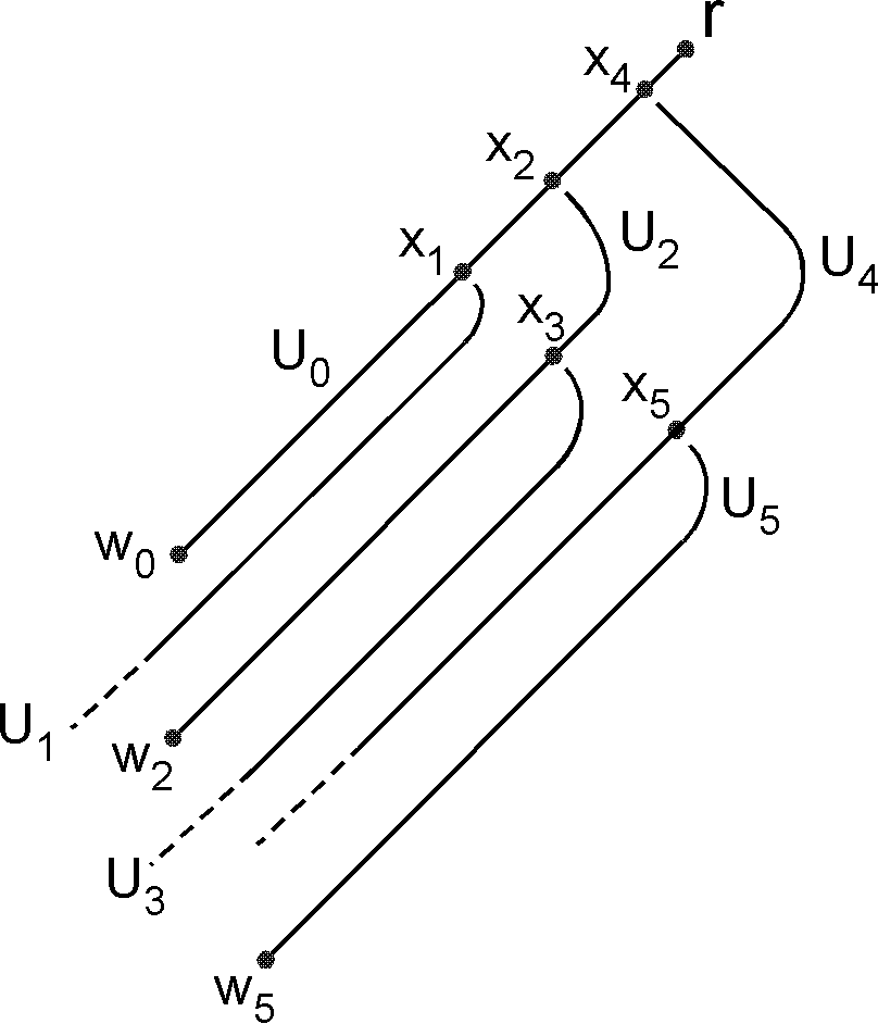
Figure 1. A structured binary join-tree.

Proposition 2.

Every join-tree and, more generally, every join-forest has a structuring.

Proof 3.1.

Let $J=(N,\leq)$ be a join-tree. Let us choose an enumeration of $N$ and a maximal line $B_{0}$ ; it is upwards closed. For each $i>0$, we choose a maximal line $B_{i}$ containing the first node not in $B_{i-1}\cup\dots\cup B_{0}$. We define $U_{0}:=B_{0}$ and, for $i>0$, $U_{i}:=B_{i}-(U_{i-1}\uplus\dots\uplus U_{0})=B_{i}-(B_{i-1}\cup\dots\cup B_{0})$. We define $\mathcal{U}$ as the set of lines $U_{i}$. It is a structuring of $J$. The axis is $U_{0}$. If $J$ is a join-forest, it has a structuring that is the union of structurings of its components.

Remark. Since each line $B_{i}$ is maximal, if $U_{i}$ has a smallest element, this element is a node of degree 0 in $J$.

In view of our use of monadic second-order logic, we give a description of SJ-trees by relational structures.

[SJ-trees as relational structures]

If $J=(N,\leq,\mathcal{U})$ is an SJ-tree, we define $S(J)$ as the relational structure $(N,\leq,N_{0},N_{1})$ such that $N_{0}$ is the set of nodes at even depth and $N_{1}:=N-N_{0}$ is the set of those at odd depth. ($N_{0}$ and $N_{1}$ are sets but we will also consider them as unary relations).

Proposition 3.

1. There is an MS formula $\varphi(N_{0},N_{1})$ expressing that a relational structure $(N,\leq,N_{0},N_{1})$ is $S(J)$ for some SJ-tree $J=(N,\leq,\mathcal{U})$.

2. There exist MS formulas $\theta_{Ax}(X,N_{0},N_{1})$ and $\theta(u,U,N_{0},N_{1})$ expressing, respectively, in a structure $(N,\leq,N_{0},N_{1})=S((N,\leq,\mathcal{U})),$ that $X$ is the axis and that $U\in\mathcal{U}\wedge u=\widehat{U}$.

Proof 3.2.

Let $J=(N,\leq)$ be a join-tree and $X\subseteq N$. We say that $X$ is laminar if, for all $x,y,z\in X$, if $[x,z]\cup[y,z]\subseteq X$ (where $x<z$ and $y<z),$ then $[x,z]\subseteq[y,z]$ or $[y,z]\subseteq[x,z]$ (the intervals $[x,z]$ and $[y,z]$ are relative to $J$). This condition implies that the lines of $J$ that are included in $X$ and are maximal with this condition form a partition of $X$ whose parts will be called its components.

It is clear from the definitions that, if $J=(N,\leq,\mathcal{U})$ is an SJ-tree and $S(J)=(N,\leq,$ $N_{0},N_{1})$, then the sets $N_{0}$ and $N_{1}$ are laminar, $\mathcal{U}$ is the set of their components and the axis $A$ is a component of $N_{0}$.

1. That a partial order $(N,\leq)$ is a join-tree is first-order expressible. The formula $\varphi(N_{0},N_{1})$ will include this condition.

   Let $J=(N,\leq)$ be a join-tree, $N$ the union of two disjoint laminar sets $N_{0}$ and $N_{1},$ and $\mathcal{U}$ the set of their components. Then, $J=(N,\leq,\mathcal{U})$ is an SJ-tree such that $S(J)=(N,\leq,N_{0},N_{1})$ if and only if:

   1. every component of $N_{1}$ has a top in $N_{0}$ and every component of $N_{0}$ except one has a top in $N_{1}$,

   2. for each $U$ in $\mathcal{U}$, the sequence $U_{0},U_{1},\dots$ of lines of $\mathcal{U}$ such that $U_{0}=U$, $\widehat{U_{0}}\in U_{1},\dots,\widehat{U_{i}}\in U_{i+1}$ terminates at some $U_{k}$ that has no top, hence is included in $N_{0}$.

   These conditions are necessary. As they rephrase Definition 3.1, they are also sufficient. The integer $k$ in Condition (ii) is the common depth of all nodes in $U$.

   That a set $X$ is laminar is first-order expressible, and one can build an MS formula $\psi(U,X)$ expressing that $U$ is a component of $X$ assumed to be laminar. This formula can be used to express that $N$ is the union of two disjoint laminar sets $N_{0}$ and $N_{1}$ that satisfy Conditions (i) and (ii). For expressing Condition (ii), we define, for each $U$ in $\mathcal{U}$, a set of nodes $W$ as follows: it is the least set such that $\widehat{U}\in W,$ and, for each $w\in W$, the top of $U(w)$ belongs to $W$ if it is defined (where $U(w)$ is the unique set in $\mathcal{U}$ that contains $w$). The set $W$ is linearly ordered (it consists of $\widehat{U_{0}}<\dots<\widehat{U_{i}}\dots$) and Condition (ii) says that it must be finite. To write the formula, we use the observation made in Section 2 that the finiteness of a linearly ordered set is MS expressible.

2. The construction of $\varphi$ actually uses the MS formulas $\theta_{Ax}(X,N_{0},N_{1})$ and $\theta(u,U,N_{0},N_{1})$.

3.2. Description schemes of structured binary join-trees

In order to introduce technicalities step by step, we first consider binary join-trees. They are actually sufficient for defining the rank-width of a countable graph. See Section 5.

[Structured binary join-trees]

Let $J=(N,\leq)$ be a binary join-tree, a BJ-tree in short. A structuring of $J$ is a set $\mathcal{U}$ of lines satisfying the conditions of Definition 3.1 and, furthermore:

1. if the axis $A$ has a smallest element, then its degree is 0 or 1,

2. each $x\in N$ is the top of at most one set $U\in\mathcal{U}$, denoted by $U^{x}$, and $U^{x}:=\emptyset$ if $x$ is the top of no $U\in\mathcal{U}$.

We call $(N,\leq,\mathcal{U})$ a structured binary join-tree, an SBJ-tree in short.

Proposition 4.

1. Every BJ-tree $J$ has a structuring.

2. The class of stuctures $S(J)$ for SBJ-trees $J$ is monadic second-order definable.

Proof 3.3.

1. We use the construction of Proposition 2 for $J=(N,\leq)$. The remark following it implies that, if the axis $A=U_{0}$ has a smallest element, this element has degree 0. It implies also that, if $\widehat{U_{i}}=x$, then $x$ cannot have degree 0 in the BJ-tree $J_{i-1}$ induced by $U_{i-1}\uplus\dots\uplus U_{0}$ because each line $B_{i}$ is chosen maximal; furthermore, it cannot have degree 2 or more in $J_{i-1}$ because $J$ is binary. Hence it has degree 1 in $J_{i-1}$. It follows that $x$ is the top of no line $U_{j}$ for $j<i$. Hence (ii) holds and the construction yields an SBJ-tree $(N,\leq,\mathcal{U})$.

2. The formula $\varphi$ of Proposition 3 can be modified so as to express that ${(N,\leq,}N_{0},N_{1})$ is $S(J)$ for some SBJ-tree $J.$

[Description schemes for SBJ-trees]

1. A description scheme for an SBJ-tree, in short an SBJ-scheme, is a triple $\Delta=(Q,w_{Ax},(w_{q})_{q\in Q})$ such that $Q$ is a set called the set of states, $w_{Ax}\in\mathcal{A}(Q)$ (is an arrangement over $Q$) and $w_{q}\in\mathcal{A}(Q)$ for each $q$. It is regular if $Q$ is finite and the arrangements $w_{Ax}$ and $w_{q}$ are regular.

2. We recall that a linear order $(V,\leq)$ is identified with the arrangement $(V,\leq,Id)$. If $W\subseteq V$ and $r:V\rightarrow Q$, then $\overline{r}((W,\leq))$ is the arrangement $(W,\leq\upharpoonright W,r\upharpoonright W)\in\mathcal{A}(Q)$ that we will denote more simply by $(W,\leq,r)$ leaving implicit the restrictions of $\leq$ and $r$ to $W$.

   An SBJ-scheme $\Delta$ describes an SBJ-tree $J=(N,\leq,\mathcal{U})$ whose axis is $A$ if there exists a mapping $r:N\rightarrow Q$ that we call a run, such that:

   $$\overline{r}((A,\leq))\simeq w_{Ax}\text{ and }\overline{r}((U^{x},\leq))\simeq w_{r(x)}\text{ for every }x\in N.$$

   We will also say that $\Delta$ describes the BJ-tree $\mathit{fgs}(J):=(N,\leq)$, where $\mathit{fgs}$ makes an SBJ-tree into a BJ-tree by forgetting its structuring. The mapping $r$ need not be surjective, this means that some elements of $Q$ and the corresponding arrangements may be useless, and thus can be removed from $\Delta$.

Figure 2. A binary join-tree.

For an example, let $\Delta=(Q,w_{Ax},(w_{q})_{q\in Q})$ be the SBJ-scheme such that $Q=\{a,b,c\}$, $w_{Ax}:=(\mathbb{Z},\leq,\ell)$ where $\ell(i)=a$ if $i$ is even and $\ell(i)=b$ if $i$ is odd, $w_{a}:=\{c\},w_{b}:=cc$ (two nodes labelled by $c$) and $w_{c}=\Omega.$ It describes the BJ-tree of Figure 2.

Proposition 5.

1. Every SBJ–tree is descibed by some SBJ-scheme.

2. Every SBJ-scheme $\Delta$ describes a unique SBJ-tree, where unicity is up to isomorphism.

Proof 3.4.

1. Each SBJ-tree $J=(N,\leq,\mathcal{U})$ has a standard description scheme

   $$\Delta(J):=(N,(A,\leq),((U^{x},\leq))_{x\in N}).$$

   The run is the identity mapping $r:N\rightarrow N$ showing that $\Delta(J)$ describes $J$.

2. We will denote by $\mathit{Unf}(\Delta)$ the SBJ-tree described by $\Delta$ and call it called the unfolding of $\Delta$ (see the remark following the proof about terminology). Let $\Delta=(Q,w_{Ax},(w_{q})_{q\in Q})$ be an SBJ-scheme, defined with arrangements $w_{Ax}=(V_{Ax},$ $\preceq,lab_{Ax})$ and $w_{q}=(V_{q},\preceq,lab_{q})$ such that, without loss of generality, the sets $V_{Ax}$ and $V_{q}$ are pairwise disjoint and the same symbol $\preceq$ denotes their orders. We construct $(N,\leq,\mathcal{U})=\mathit{Unf}(\Delta)$ as follows.

   1. $N$ is the set of finite nonempty sequences $(v_{0},v_{1},\dots,v_{k})$ such that $v_{0}\in V_{Ax},v_{i}\in V_{q_{i}}$ for $1\leq i\leq k$, where $q_{1}=lab_{Ax}(v_{0})$, $q_{2}=lab_{q_{1}}(v_{1})$, …, $q_{k}=lab_{q_{k-1}}(v_{k-1})$.

   2. $(v_{0},v_{1},\dots,v_{k})\leq(v_{0}^{\prime},v_{1}^{\prime},\dots,v_{j}^{\prime})$ if and only if $k\geq j$, $(v_{0},v_{1},\dots,v_{j-1})=(v_{0}^{\prime},v_{1}^{\prime},\dots,$ $v_{j-1}^{\prime})$ and $v_{j}\preceq v_{j}^{\prime}.$

   3. The axis $A$ is the set of one-element sequences $(v)$ for $v\in V_{Ax}$; for $x=(v_{0},v_{1},\dots,v_{k}),$ we define $U(x)$ as the set of sequences $(v_{0},v_{1},\dots,v_{k-1},v)$ such that $v\in V_{q_{k}}$, hence, we have $\widehat{U(x)}=(v_{0},v_{1},\dots,v_{k-1}).$

   Note that $(v_{0},\dots,v_{k})<(v_{0},\dots,v_{j})$ if $j<k$ and that $(v_{0},\dots,v_{k-1},v_{k})\leq(v_{0},\dots,v_{k-1},v)$ if and only if $v_{k}\preceq v$. We claim that $\Delta$ describes $(N,\leq,\mathcal{U})$. For proving that, we define a run $r:N\rightarrow Q$ as follows:

   • if $x\in A$, then $x=(v)$ for some $v\in V_{Ax}$ and $r(x):=lab_{Ax}(v);$

   • if $x\in N$ has depth $k\geq 1$, then $x=(v_{0},v_{1},\dots,v_{k})$ for some $v_{0},v_{1},\dots,v_{k}$ as in (a) and $r(x):=lab_{q_{k}}(v_{k})$.

   It follows that $\overline{r}((A,\leq))\simeq w_{Ax}$ and that, for $x=(v_{0},v_{1},\dots,v_{k})$ (of depth $k$), we have $\overline{r}((U^{x},\leq))\simeq w_{q_{k}}=w_{r(x)}$, which proves the claim.

   We now prove unicity. Assume that $\Delta$ describes $J=(N,\leq,\mathcal{U})$ with axis $A$ and also $J^{\prime}=(N^{\prime},\leq^{\prime},\mathcal{U}^{\prime})$ with axis $A^{\prime}$, by means of runs $r:N\rightarrow Q$ and $r^{\prime}:N^{\prime}\rightarrow Q$. We construct an isomorphism $h:J\rightarrow J^{\prime}$ as the common extension of bijections $h_{k}:N_{k}\rightarrow N_{k}^{\prime}$, where $N_{k}$ (resp. $N_{k}^{\prime}$) is the set of nodes of $J$ (resp. of $J^{\prime}$) of depth at most $k,$ and such that they map $\leq$ to $\leq^{\prime},$ and the lines of $\mathcal{U}$ to those of $\mathcal{U}^{\prime}$ of same depth, and finally, $r^{\prime}\circ h_{k}=r\upharpoonright N_{k}.$

   • Case $k=0$. We have:

     $$\overline{r}((A,\leq))=(A,\leq,r)\simeq w_{Ax}\simeq\overline{r^{\prime}}((A^{\prime},\leq))=(A^{\prime},\leq^{\prime},r^{\prime})$$

     which gives the order preserving bijection $h_{0}:N_{0}=A\rightarrow N_{0}^{\prime}=A^{\prime}$ such that $r^{\prime}\circ h_{0}=r\upharpoonright N_{0}.$

   • Case $k>0$. We assume inductively that $h_{k-1}$ has been constructed.

     Let $U\in\mathcal{U}$ be such that $x=\widehat{U}$ has depth $k-1$; hence, $U\cap N_{k-1}=\emptyset.$ Then $(U,\leq,r)\simeq w_{r(x)}.$ Let $x^{\prime}=h_{k-1}(x)$; we have $r^{\prime}(x^{\prime})=r(x)$. Hence there is $U^{\prime}\in\mathcal{U}^{\prime}$ such that $x^{\prime}=\widehat{U^{\prime}}$, $U^{\prime}\cap N_{k-1}^{\prime}=\emptyset$ and$(U^{\prime},\leq^{\prime},r^{\prime})\simeq w_{r^{\prime}(x^{\prime})}=w_{r(x)}$. Hence, there is an order preserving bijection $h_{U}:U\rightarrow U^{\prime}$ such that $r^{\prime}\circ h_{U}=r\upharpoonright U.$

     We define $h_{k}$ as the common extension of the injective mappings $h_{k-1}$ and $h_{U}$ such that $U\in\mathcal{U}$ and the depth of $\widehat{U}$ is $k-1$. These mappings have pairwise disjoint domains whose union is $N_{k}$.

   The extension to $N$ of all these mappings $h_{k}$ is the desired isomorphism $h$.

Remarks.

1. We call unfolding the transformation of $\Delta$ into $\mathit{Unf}(\Delta)$ because it generalizes the unfolding of a directed graph $G$ into a finite or countable rooted tree. The unfolding is done from a particular vertex $s$ of $G$, and the nodes of the tree are the sequences of the form $(x_{0},\dots,x_{k})$ such that $s=x_{0}$ and there is a directed edge in $G$ from $x_{i}$ to $x_{i+1}$, for each $i<k$. If $\Delta$ is such that the arrangements $w_{Ax}$ and $w_{q}$ are reduced to a single element, the corresponding directed graph has all its vertices of outdegree one and the tree resulting from the unfolding consists of one infinite path: the SBJ-tree $\mathit{Unf}(\Delta)$ is the order type $\omega^{-}$ of negative integers and the sets in $\mathcal{U}$ are singletons.

   
   

2. An SBJ-scheme $\Delta$ describing an SBJ-tree $J$ can be seen as a quotient of $\Delta(J).$ We define quotients in terms of surjective mappings.

   Let $\Delta=(Q,w_{Ax},(w_{q})_{q\in Q})$ and $s:Q\rightarrow Q^{\prime}$ be surjective such that, if $s(q)=s(q^{\prime})$, then $\overline{s}(w_{q})\simeq\overline{s}(w_{q^{\prime}})$. We define $\Delta^{\prime}:=(Q^{\prime},\overline{s}(w_{Ax}),(w_{p}^{\prime})_{p\in Q^{\prime}})$ where $w_{s(q)}^{\prime}\simeq\overline{s}(w_{q})$ for each $q$ in $Q$. If $\Delta$ describes $J$ via a run $r:N\rightarrow Q$, then $\Delta^{\prime}$ describes $J$ via $s\circ r:N\rightarrow Q^{\prime}$. We say that $\Delta^{\prime}$ is the quotient of $\Delta$ by the equivalence $\thickapprox$ on $Q$ such that $q\approx q^{\prime}$ if and only if $s(q)=s(q^{\prime})$, and we denote it by $\Delta/\thickapprox$. If $\Delta$ is regular, then $\Delta/\thickapprox$ is regular and its set of sates is smaller than that of $\Delta$ unless $s$ is a bijection.

   Let us now start from an SBJ-tree $J=(N,\leq,\mathcal{U})$ with axis $A$. For $x\in N$, let $J_{x}$ be the SBJ-tree $(N_{x},\leq_{x},\mathcal{U}_{x})$ such that $N_{x}:=\mathord{\downarrow}(U^{x}),\leq_{x}$ is the restriction of $\leq$ to $N_{x}$, and $\mathcal{U}_{x}:=\{U^{x}\}\cup\{U^{y}\mid y\in N_{x}\}-\{\emptyset\}$. Its axis is $U^{x}$. For the example of Figure 1, we have $\mathcal{U}_{x_{2}}=\{U_{2},U_{3}\}$ and $U_{2}$ is the axis.

   From J, we define as follows a canonical SBJ-scheme $\Delta(J)/\thickapprox$ based on the equivalence $\thickapprox$ on $N$ such that $x\approx x^{\prime}$ if and only if $J_{x}\simeq J_{x^{\prime}}$. Let $s$ be the surjective mapping : $N\rightarrow N^{\prime}:=N/\approx$. If $J_{x}\simeq J_{y}$ by an isomorphism $h:N_{x}\rightarrow N_{y}$, then $(U^{x},\leq)\simeq(U^{y},\leq)$ by $h\upharpoonright U^{x}:U^{x}\rightarrow U^{y}$ and furthermore, if $w\in N_{x}$, then $J_{w}\simeq J_{h(w)}$ by $h\upharpoonright N_{w}:N_{w}\rightarrow N_{h(w)}$. It follows that $\overline{s}((U^{x},\leq))\simeq\overline{s}((U^{y},\leq)),$ hence, the quotient SBJ-scheme $\Delta(J)/\thickapprox:=(N^{\prime},\overline{s}((A,\leq)),(w_{p}^{\prime})_{p\in N^{\prime}})$ such that $w_{p}^{\prime}\simeq$ $\overline{s}((U^{x},\leq))$ if $s(x)=p$ is well-defined and describes $J$.

   Let $\Delta=(Q,w_{Ax},(w_{q})_{q\in Q})$ describe $J$ via a surjective run $r:N\rightarrow Q$ and consider the equivalence relation on $Q$ such that $q\equiv q^{\prime}$ if and only if there exist $x,y$ such that $r(x)=q$, $r(y)=q^{\prime}$ and $J_{x}\simeq J_{y}$. It is well-defined because if $r(x)=r(y)=q$, then $\overline{r}((U^{x},\leq))\simeq\overline{r}((U^{y},\leq))\simeq w_{q},$ and furthermore $J_{x}\simeq J_{y}$: one constructs an isomorphism $h$ that extends the one between $\overline{r}((U^{x},\leq))$ and $\overline{r}((U^{y},\leq))$ (this construction uses an induction on the depth of $u$ in $J_{x}$ for defining $h(u)$). Hence, $\Delta/\equiv$ is well-defined and describe $J$ via the run $r^{\prime}$ such that $r^{\prime}(x)$ is the equivalence class of $r(x)$ with respect to $\equiv.$ It follows that $\Delta/\equiv$ is isomorphic to $\Delta(J)/\thickapprox.$ If $J$ is regular, then $\Delta(J)/\thickapprox$ is the unique regular SBJ-scheme describing $J$ that has a minimum number of states. As usual, unicity is up to isomorphism. This construction is similar to that of the minimal deterministic automaton of a regular language, defined from its quotients (see e.g., [26], chapter I.3.3).

Proposition 6.

A BJ-tree is monadic second-order definable if it is described by a regular SBJ-scheme.

Proof 3.5.

That $J=(N,\leq)$ is a BJ-tree is first-order expressible. Assume that $J=\mathit{fgs}(J^{\prime})$ where $J^{\prime}=(N,\leq,\mathcal{U})\simeq\mathit{Unf}(\Delta)$ for some regular SBJ-scheme $\Delta=(Q,w_{Ax},(w_{q})_{q\in Q})$ such that $Q=\{1,\dots,m\}$. Let $r$ be the corresponding mapping: $N\rightarrow Q$ (cf. Definition 3.3(b)). For each $q\in Q$, let $\psi_{q}$ be an MS sentence that characterizes $w_{q}$, up to isomorphism, by the main result of [23]. Similarly, $\psi_{Ax}$ characterizes $w_{Ax}$. We claim that a relational structure $(X,\leq)$ is isomorphic to $J$ if and only if there exist subsets $N_{0},N_{1},M_{1},\dots,M_{m}$ of $X$ such that:

1. $(X,\leq)$ is a BJ-tree and $(X,\leq,N_{0},N_{1})=S(J^{\prime\prime})$ for some SBJ-tree $J^{\prime\prime}=(X,\leq,\mathcal{U}^{\prime})$,

2. $(M_{1},\dots,M_{m})$ is a partition of $X$; we let $r^{\prime}$ maps each $x\in X$ to the unique $q\in Q$ such that $x\in M_{q},$

3. for every $q\in Q$ and $x\in M_{q}$, the arrangement $\overline{r^{\prime}}((U^{x},\leq))$ over $Q$ (where $U^{x}\in\mathcal{U}^{\prime})$ is isomorphic to $w_{q},$

4. the arrangement $\overline{r^{\prime}}((A^{\prime},\leq))$ over $Q$ where $A^{\prime}$ is the axis of $J^{\prime\prime}$ is isomorphic to $w_{Ax}$.

Conditions (ii)-(iv) express that $\Delta$ describes $J^{\prime\prime}$, hence that $J^{\prime\prime}$ is isomorphic to $J^{\prime},$ and so that $(X,\leq)\simeq\mathit{fgs}(J^{\prime})=J$.

By Proposition 4, Condition (i) is expressed by an MS formula $\varphi(N_{0},N_{1})$, and the property $U\in\mathcal{U}\wedge x=\widehat{U}$ is expressed in terms of $N_{0},N_{1}$ by an MS formula $\theta(x,U,N_{0},N_{1}).$ Conditions (iii) and (iv) are expressed by means of the MS sentences $\psi_{Ax}$ and $\psi_{q}$ suitably adapted to take $N_{0},N_{1},M_{1},\dots,M_{m}$ as arguments. Hence, $J$ is (up to isomorphism) the unique model of an MS sentence of the form:

$$\exists N_{0},N_{1}.\left[\varphi(N_{0},N_{1})\wedge\exists M_{1},\dots,M_{m}.\varphi^{\prime}(N_{0},N_{1},M_{1},\dots,M_{m})\right]$$

where $\varphi^{\prime}$ expresses conditions (ii)-(iv).

Theorem 9 will establish a converse.

3.3. The algebra of binary join-trees

We define three operations on structured binary join-trees (SBJ-trees in short). The finite and infinite terms over these operations will define all SBJ-trees.

[Operations on SBJ-trees]

• Concatenation along axes.

  Let $J=(N,\leq,\mathcal{U})$ and $J^{\prime}=(N^{\prime},\leq^{\prime},\mathcal{U}^{\prime})$ be disjoint SBJ-trees, with respective axes $A$ and $A^{\prime}$. We define:

  $$J\bullet J^{\prime} :=(N\uplus N^{\prime},\leq^{\prime\prime},\mathcal{U}^{\prime\prime})\text{ where }$$

  $$x\leq^{\prime\prime}y :\Longleftrightarrow x\leq y\vee x\leq^{\prime}y\vee(x\in N\wedge y\in A^{\prime}),$$

  $$\mathcal{U}^{\prime\prime} :=\{A\uplus A^{\prime}\}\uplus(\mathcal{U-}\{A\}\mathcal{)}\uplus(\mathcal{U}^{\prime}\mathcal{-}\{A^{\prime}\}\mathcal{)}.$$

  It follows that $J\bullet J^{\prime}$ is an SBJ-tree with axis $A\uplus A^{\prime}$; the depth of a node in $J\bullet J^{\prime}$ is the same as in $J$ or $J^{\prime}$. This operation generalizes the concatenation of linear orders: if $(N,\leq)$ and $(N^{\prime},\leq^{\prime})$ are disjoint linear orders, then the SBJ-tree $(N,\leq,\{N\})\bullet\left(N^{\prime},\leq^{\prime},\{N^{\prime}\}\right)$ corresponds to the concatenation of $(N,\leq)$ and $\left(N^{\prime},\leq^{\prime}\right)$ usually denoted by $(N,\leq)+\left(N^{\prime},\leq^{\prime}\right)$, cf. [20]. If $K=(M,\leq,\mathcal{V})$ is an SBJ-tree with axis $B$, and $B=A\uplus A^{\prime}$ such that $A<A^{\prime},$ then $K=J\bullet J^{\prime}$ where:

  • $N:=\downarrow(A),N^{\prime}:=M-N,$

  • $\mathcal{U}$ is the set of lines of $\mathcal{V}$ included in $N-A$ together with $A,$

  • $\mathcal{U}^{\prime}$ is the set of lines of $\mathcal{V}$ included in $N^{\prime}-A^{\prime}$ together with $A^{\prime}$ and

  • the orders of $J$ and $J^{\prime}$ are the restrictions of $\leq$ to $N$ and $N^{\prime}$.

• The empty SBJ-tree.

  The nullary symbol $\Omega$ denotes the empty SBJ-tree.

• Extension.

  Let $J=(N,\leq,\mathcal{U})$ be an SBJ-tree, and $u\notin N$. Then:

  $$ext_{u}(J) :=(N\uplus\{u\},\leq^{\prime},\{\{u\}\}\uplus\mathcal{U})\text{ where }$$

  $$x\leq^{\prime}y :\Longleftrightarrow x\leq y\vee y=u,$$

  the axis is $\{u\}$. Clearly, $ext_{u}(J)$ is an SBJ-tree. The depth of $v\in N$ is its depth in $J$ plus 1. The axis of $J$ is turned into an “ordinary line” of the structuring of $ext_{u}(J)$ with top equal to $u$. When handling SBJ-trees up to isomorphism, we use the notation $ext(J)$ instead of $ext_{u}(J).$

• Forgetting structuring.

  If $J$ is an SBJ-tree as above, $\mathit{fgs}(J):=(N,\leq)$ is the underlying BJ-tree (binary join-tree), where $\mathit{fgs}$ forgets the structuring.

Anticipating the sequel, we observe that a linear order $a_{1}<\dots<a_{n}$, identified with the SBJ-tree $(\{a_{1},\dots,a_{n}\},\leq,\{\{a_{1},\dots,a_{n}\}\})$ is defined by the term $t:=ext_{a_{1}}(\Omega)\bullet ext_{a_{2}}(\Omega)\bullet\dots\bullet ext_{a_{n}}(\Omega).$ The binary (it is even “unary”) join-tree $(\{a_{1},\dots,a_{n}\},\leq)$ is defined by the term $\mathit{fgs}(t)$ and also, in a different way, by the term $\mathit{fgs}(ext_{a_{n}}(ext_{a_{n-1}}(\dots(ext_{a_{1}}(\Omega)))..)))$.

[The algebra $\mathbb{SBJT}$]

We let $F$ be the signature $\{\bullet,ext,\Omega\}$. We obtain an algebra $\mathbb{SBJT}$ whose domain is the set of isomorphism classes of SBJ-trees. Concatenation is associative with neutral element $\Omega$.

[The value of a term]

1. In order to define the value of a term $t$ in $T^{\infty}(F)$, we compare its positions by the following equivalence relation:

   $u\approx v$ if and only if every position $w$ such that $u<_{t}w\leq_{t}u\sqcup_{t}v$ or $v<_{t}w\leq_{t}u\sqcup_{t}v$ is an occurrence of $\bullet$.

   We will also use the lexicographic order $\leq_{lex}$ (positions are Dewey words). If $w$ is an occurrence of a binary symbol, then $s_{1}(w)$ is its first (left) son and $s_{2}(w)$ its second (right) one.

2. We define the value $val(t):=(N,\leq,\mathcal{U})$ of $t$ in $T^{\infty}(F)$ as follows:

   • $N:=\mathrm{Occ}(t,ext)$, the set of occurences in $t$ of $ext$,

   • $u\leq v:\Longleftrightarrow u\leq_{t}w\leq_{lex}v$ for some $w\in N$ such that $w\approx v,$

   • $\mathcal{U}$ is the set of equivalence classes of $\approx.$

   Equivalently, we have:

   $u\leq v:\Longleftrightarrow u\leq_{t}v$ or $u\leq_{t}s_{1}(u\sqcup_{t}v),$ $v\leq_{t}s_{2}(u\sqcup_{t}v)$ and $v\approx u\sqcup_{t}v$ (the position $u\sqcup_{t}v$ is an occurrence of $\bullet$),

   and so (we recall that $\bot$ denotes incomparability):

   $u\bot v:\Longleftrightarrow u\leq_{t}s_{1}(u\sqcup_{t}v),$ $v\leq_{t}s_{2}(u\sqcup_{t}v)$ and there is an occurrence of $ext$ between $v$ and $u\sqcup_{t}v$ or vice-versa by exchanging $u$ and $v$.

3. We now consider terms $t$ written with the operations $ext_{a}$ (such that $a$ is the node created by applying this operation). For each $a$, the operation $ext_{a}$ must have at most one occurrence in $t$. Assuming this condition satisfied, then $val(t):=(N,\leq,\mathcal{U})$, where

   • $N$ is the set of nodes $a$ such that $ext_{a}$ has an occurence in $t$ that we will denote by $u_{a}$,

   • $a\approx b:\Longleftrightarrow u_{a}\approx u_{b}$, with $\approx$ as in (a),

   • $a\leq b:\Longleftrightarrow u_{a}\leq u_{b}$, with $\leq$ as in (b),

   • $\mathcal{U}$ is the set of equivalence classes of $\approx.$

   Clearly, the mapping $val$ in (b) is a value mapping $T^{\infty}(F)\rightarrow\mathbb{SBJT}$.

We say that $t$ denotes an SBJ-tree $J$ if $J$ is isomorphic to $val(t)$, and, in this case, we also say that $\mathit{fgs}(t)$ denotes the BJ-tree $\mathit{fgs}(J)$.

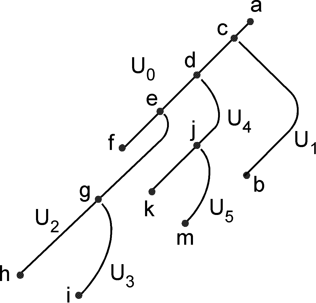
Figure 3. A finite SBJ-tree $J$.

Note that we do not define the value of term as the least upper bound of the values of its finite subterms. We could use a notion of least upper bound based on category theory as in [8], at the cost of heavy definitions. Our simpler definition shows furthermore that the mapping associating the join-tree $(N,\leq)$ with $\left\lfloor t\right\rfloor$ for $t\in T^{\infty}(F)$ is an MS-transduction (cf. Section 2) defined by $\mathcal{D}=\langle\chi,\delta,\theta_{\leq}\rangle$ where $\chi$ expresses that the considered input structure $S$ is isomorphic to $\left\lfloor t\right\rfloor$ for some $t\in T^{\infty}(F),$ $\delta(x)$ is $lab_{ext}(x)$ (expressing that $x\in N)$ and $\theta_{\leq}(x,y)$ expresses that $x\leq y$, cf. Definition 3.3(b).

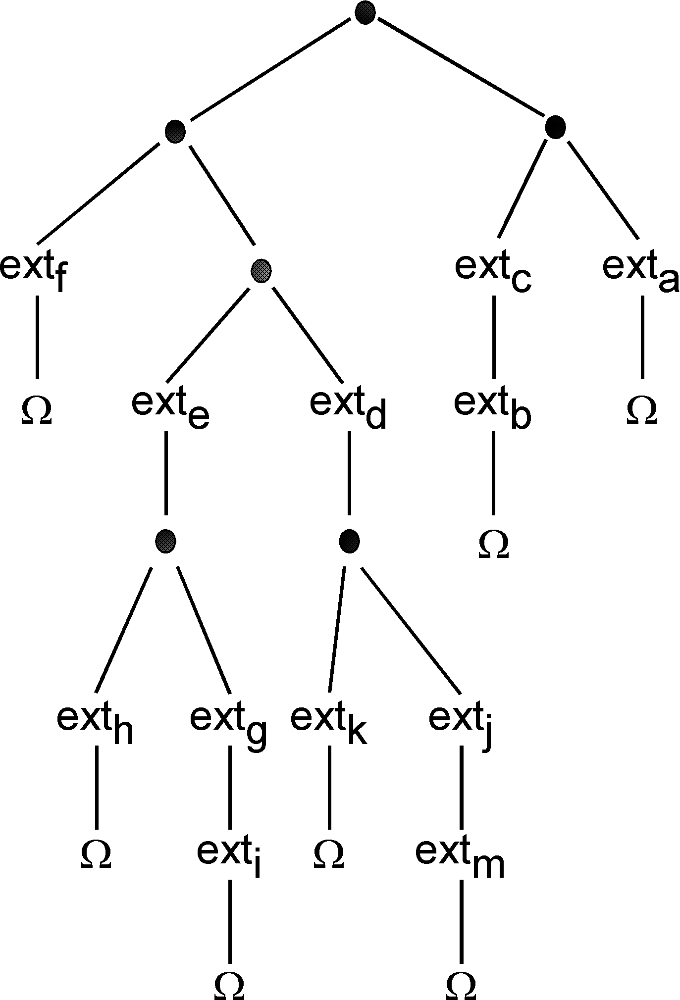
Figure 4. A term $t$ denoting $J$.

1. The term $t_{0}$ that is the unique solution in $T^{\infty}(F)$ of the equation $t_{0}=t_{0}\bullet t_{0}$ denotes the empty SBJ-tree $\Omega$.

2. Figure 3 shows a finite SBJ-tree $J$ whose structuring consists of $U_{0},\dots,U_{5}$, and $U_{0}$ is the axis. The linear order on $U_{0}$ can be described by the word $fedca$ (with $f<e<d<\dots).$ Similarly, $U_{1}=b,U_{2}=hg,U_{3}=i$ , $U_{4}=kj$ and $U_{5}=m$.

   Let us examine the term $t$ of Figure 4 that denotes $J$. A function symbol $ext_{u}$ specifies the node $u$ of $J$, and we also denote by $u$ its occurrence, a position of $t$ (hence b denotes position 21). The occurrences of $\bullet$ and $\Omega$ are denoted by Dewey words. For example, the occurrences of $\bullet$ above the symbols $ext$ are the words $\varepsilon,1,2,12$. The set $\{\varepsilon,1,2,12,f,e,d,c,a\}$ is an equivalence class of $\approx$. Another one is $\{1221,k,j\}$. Each line $U_{i}$ is the set of positions of the $ext$ symbols in some equivalence class of $\approx$. Let us now examine how each line is ordered.

   The case where $u<v$ holds because $u<_{t}v$ is illustrated, to take a few cases, by $i<g,g<e,m<j$ and $j<d$. The case where $u<v$ holds because $u\bot_{t}v$, $u\leq_{t}s_{1}(u\sqcup_{t}v),$ $v\leq_{t}s_{2}(u\sqcup_{t}v)$ and $v\approx u\sqcup_{t}v$ is illustrated by $f<e,e<d,d<c$ and $i<d$. We have $i<d$ because $i\sqcup_{t}d=12,$ $i<_{t}s_{1}(12),$ $d\leq_{t}s_{2}(12)$ and $d\approx 12$. We do not have $i<j$ because $j$ is not $\approx$-equivalent to 12, whereas $i\sqcup_{t}j=12,$ $i<_{t}s_{1}(12)$ and $j\leq_{t}s_{2}(12)$. This case illustrates the characterization of $\bot$ Definition 3.3(c).

   

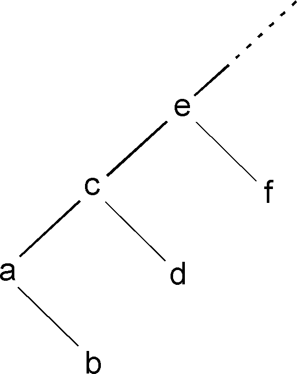
   Figure 5. The SBJ-tree $val(t_{1})$.

3. Let $t_{1}$ be the solution in $T^{\infty}(F)$ of the equation $t_{1}=ext(ext(\Omega))\bullet t_{1}$. We write it by naming $a,a^{\prime},b,b^{\prime},c,c^{\prime}\dots$ the nodes created by the operations $ext$, hence, t${}_{1}=ext_{a}(ext_{a^{\prime}}(\Omega))\bullet(ext_{b}(ext_{b^{\prime}}(\Omega))\bullet(ext_{c}(ext_{c^{\prime}}(\Omega))\bullet\dots))).$ This term and its value are shown in Figure 5. The bold edges link nodes in the axis. The nodes $a^{\prime}$ and $c^{\prime}$ are incomparable because the corresponding occurrences of $ext,$ that are 111 and 2211, have least common ancestor $\varepsilon$ and 221 is an occurrence of $ext$ between 2211 and $\varepsilon$.

4. The following BJ-tree is defined by Fraïssé in [16] (Section 10.5.3). We let $W:=(Seq_{+}(\mathbb{Q}),\preceq)$ where $Seq_{+}(\mathbb{Q})$ is the set of nonempty sequences of rational numbers, partially ordered as follows:$(x_{n},\dots,x_{0})\preceq(y_{m},\dots,y_{0})$ if and only if $n\geq m$, $(x_{m-1},\dots,x_{0})=(y_{m-1},\dots,y_{0})$ and $x_{m}\leq y_{m}$. In particular, $\prec$ is the transitive closure of $\prec_{0}\cup\prec_{1}$ where $(x_{p+1},x_{p},\dots,x_{0})\prec_{0}(x_{p},\dots,x_{0})$ and $(y,x_{p-1},\dots,x_{0})\prec_{1}(z,x_{p-1},\dots,x_{0})$ if $y<z.$ It is easy to check that $W$ is a BJ-tree. In particular, two nodes $(x_{n},\dots,x_{0})$ and $(y_{m},\dots,y_{0})$ are incomparable if and only if $(y_{m},\dots,y_{0})=(y_{m},\dots,y_{p+1},x_{p},\dots,x_{0})$ and $y_{p+1}\neq x_{p+1}$ for some $p<n,m.$ In this case, their join is $(\min\{y_{p+1},x_{p+1}\},x_{p},\dots,x_{0})$. The two directions relative to a node $x=(x_{p},\dots,x_{0})$ are:

   $\partial_{0}(x):=\{(y_{m},\dots,y_{p+1},x_{p},\dots,x_{0})\mid n>p,y_{m},\dots,y_{p+1}\in\mathbb{Q}\}$ and,

   $\partial_{1}(x):=\{(y_{m},\dots,y_{p+1},x_{p}^{\prime},\dots,x_{0})\mid n\geq p,x_{p}^{\prime},y_{m},\dots,y_{p+1}\in\mathbb{Q}$, $x_{p}^{\prime}<x_{p}\}$.

   A structuring $\mathcal{U}$ of $W$ consists of the sets $\{(x_{n},\dots,x_{0})\mid x_{n}\in\mathbb{Q}\}$ for each (possibly empty) sequence $(x_{n-1},\dots,x_{0})$. The set of one element sequences $(r)$ for $r\in\mathbb{Q}$ is the axis, and $U_{-}(x)\subseteq\partial_{1}(x)$ for all $x\in Seq_{+}(\mathbb{Q}).$

   The proof in [16] that every finite or countable generalized tree in the sense of [20] (i.e., partial order satisfying Condition 2) of Definition 3.1(a)) is isomorphic to $(X,\preceq\upharpoonright X)$ for some subset $X$ of $Seq_{+}(\mathbb{Q})$ uses implicitely the structuring $\mathcal{U}$. Our description of the two directions of a node shows that $W=W\bullet(ext(W)\bullet W),$ hence, that $W$ is denoted by the regular term $t\in T^{\infty}(F)$ such that $t=t\bullet(ext(t)\bullet t)$.

[The description scheme associated with a term]

1. Let $t\in T^{\infty}(F)$ and $u\in Pos(t)$. We denote by $\mathrm{Max}(t,ext,u)$ the set of maximal occurrences of $ext$ in $t$ that are below $u$ or equal to it. Positions are denoted by Dewey words, hence, these sets are linearly ordered by $\leq_{lex}$. We denote by $W(t,u)$ the simple arrangement $(\mathrm{Max}(t,ext,u),\leq_{lex}).$ Let $J=(N,\leq,\mathcal{U})$ be the value of $t$ (cf. Definition 3.3) and $x$ be an occurrence of $ext$ with son $u$. We have $(U^{x},\leq)$ $=(\mathrm{Max}(t,ext,u),\leq_{lex}).$ For the term $t$ in Example 3.3(2), see Figure 4, we have $W(t,\varepsilon)=fedca,W(t,1)=fed,W(t,1211)=hg.$ For $t_{1}$ in Example 3.3(3), we have $W(t_{1},\varepsilon)=abc\dots,W(t_{1},1)=a,W(t_{1},11)=a^{\prime}\text{ and }W(t_{1},111)=\Omega.$

2. We define $\Delta(t)$ as the SBJ-scheme $(\mathrm{Occ}(t,ext),W(t,\varepsilon),(W(t,s(x)))_{x\in\mathrm{Occ}(t,ext)})$ where $s(x)$ is the unique son of an occurrence $x$ of $ext$. We obtain

   $$\Delta(t_{1})=(\mathrm{2}^{\ast}1\uplus 2^{\ast}11,abc\dots,(w_{x})_{x\in\mathrm{Occ}(t_{1},ext)})$$

   with $w_{1}=a^{\prime}$, $w_{21}=b^{\prime}$, …, $w_{11}=\Omega$, $w_{211}=\Omega$, …for the term $t_{1}$ of Example 3.3(3).

Lemma 7.

If $t\in T^{\infty}(F),$ then $val(t)$ is described by $\Delta(t)$.

Proof 3.6.

Let $val(t)=(N,\leq,\mathcal{U}).$ The conditions of Definition 3.3(b) hold with the identity on $\mathrm{Occ}(t,ext)$ as mapping $r$ because $(U^{x},\leq)=(\mathrm{Max}(t,ext,$ $s(x)),\leq_{lex})$ as observed in Definition 4(a).

Proposition 8.

Every SBJ-tree is the value of a term.

Proof 3.7.

Let $J=(N,\leq,\mathcal{U})$ be an SBJ-tree. For each $k$, we let $J_{k}$ be the SBJ-tree $(N_{k},\leq,\mathcal{U}_{k})$ where $N_{k}$ is the set of nodes of depth at most $k$ and $\mathcal{U}_{k}$ is the set of lines $U\in\mathcal{U}$ of depth at most $k$. By induction on $k$, we define for each $k$ a term $t_{k}$ that defines $J_{k}$ such that $t_{k}$ $\underline{\ll}$ $t_{k^{\prime}}$ if $k<k^{\prime}$, and then, the least upper bound of the terms $t_{k}$ is the desired term $t$ whose value is $J$. We define terms using the symbols $ext_{a}$ where $a$ names the node created by the corresponding occurrence of the extension operation.

If $k=0$, then $J_{0}=(A,\leq,\{A\})$. There exists a term $t\in T^{\infty}(\{\bullet\},Ext_{A})$ whose value is $J_{0}$, where $Ext_{A}$ is the set of terms $ext_{a}(\Omega)$ for $a\in A$ (we use $Ext_{A}$ as a set of nullary symbols). We use here Theorem 2.3 of [8], that follows immediately from the representation of a linear order by the lexicographic order on a prefix-free language recalled in Section 1.

Let $k\geq 1$, where $t_{k-1}$ defines $J_{k-1}$. Then $J_{k}$ is obtained from $J_{k-1}$ by adding below some nodes $x$ at depth $k-1$ the line $U^{x}$ (if $U^{x}=\emptyset$, there is nothing to add below $x$). Let $t_{x}\in T^{\infty}(\{\bullet\},Ext_{U^{x}})$ whose value is $(U^{x},\leq)$. We obtain $t_{k}$ by replacing in $t_{k-1}$ each subterm $ext_{x}(\Omega)$ by $ext_{x}(t_{x})$, for $x$ at depth $k-1$ such that $U^{x}\neq\emptyset$. It is clear that $t_{k-1}$ $\underline{\ll}$ $t_{k}$ and that the least upperbound of the terms $t_{k}$ defines $J$.

For an example, we apply this construction to the SBJ-tree $J$ of Figure 3. For defining $J_{0}$, we can take:

$$t_{0}=((ext_{f}(\Omega)\bullet ext_{e}(\Omega))\bullet ext_{d}(\Omega))\bullet(ext_{c}(\Omega)\bullet ext_{a}(\Omega)).$$

To obtain $t_{1}$, we replace $ext_{e}(\Omega)$ by $ext_{e}(ext_{h}(\Omega)\bullet ext_{g}(\Omega))$, $ext_{d}(\Omega)$ by $ext_{d}(ext_{k}(\Omega)\bullet ext_{j}(\Omega))$ and $ext_{c}(\Omega)$ by $ext_{c}(ext_{b}(\Omega)),$ which gives:

$$t_{1}=((ext_{f}(\Omega)\bullet ext_{e}(ext_{h}(\Omega)\bullet ext_{g}(\Omega)))\bullet ext_{d}(ext_{k}(\Omega)\bullet ext_{j}(\Omega))\bullet(ext_{c}(ext_{b}(\Omega))\bullet ext_{a}(\Omega)).$$

Then, we obtain $t_{2}$ that defines $J$ by replacing $ext_{g}(\Omega)$ by $ext_{g}(ext_{i}(\Omega))$ and $ext_{j}(\Omega)$ by $ext_{j}(ext_{m}(\Omega)).$

3.4. Regular binary join-trees

As said in the introduction, the regular objects are those defined by regular terms. We apply this meta-definition to binary join-trees and their structurings.

[Regular BJ- and SBJ-trees]

A BJ-tree (resp. an SBJ-tree) $T$ is regular if it is denoted by $\mathit{fgs}(t)$ (resp. by $t$) where $t$ is a regular term in $T^{\infty}(F)$.

Theorem 9.

The following properties of a BJ-tree $J$ are equivalent:

1. $J$ is regular,

2. $J$ is described by a regular scheme,

3. $J$ is MS definable.

Proof 3.8.

1. $\!\!\Longrightarrow$(2) Let $J=\mathit{fgs}(J^{\prime})$ with $J^{\prime}$ denoted by a regular term $t$ in $T^{\infty}(F)$. Let $h:Pos(t)\rightarrow Q$ and $\tau$ be as in the definition of a regular term in Section 1. Without loss of generality, we can assume that $h(Pos(t))=Q$. If this is not the case, we replace $Q$ by $h(Pos(t))$ and $\tau$ by its restriction to this set.

   Claim.

   1. For each $u\in Pos(t)$, the arrangement $\overline{h}(W(t,u))=(\mathrm{Max}(t,ext,u),$ $\leq_{lex},h)$ over $Q$ is regular.

   2. If $u^{\prime}$ is another position in $t$ and $h(u^{\prime})=h(u)$, then $t/u^{\prime}=t/u$ and furthermore $\overline{h}(W(t,u^{\prime}))\simeq\overline{h}(W(t,u)).$

   Leaving its routine proof, we define $\Delta:=(Q,w_{Ax},(w_{q})_{q\in Q})$ as follows:

   1. $w_{Ax}:=$ $\overline{h}(W(t,\varepsilon))$,

   2. if $q\in Q,$ then $w_{q}:=\overline{h}(W(t,s(u)))$ where $s(u)$ is the unique son of an occurrence $u$ of $ext$ such that $h(u)=q$; if $v$ is another occurrence of $ext$ such that $h(v)=q$, then $h(s(v))=h(s(u))$ and so by the claim, $\overline{h}(W(t,s(v)))\simeq\overline{h}(W(t,s(u)))$. Hence, $w_{q}$ is well-defined up to isomorphism.

   Informally, $\Delta$ is obtained from $\Delta(t)$ by replacing the labelling mapping $Id$ of the arrangements $W(t,u)$ by $h$, so that these arrangements are turned into arrangements $\overline{h}(W(t,u))$ over $Q$. Clearly, $\Delta$ is a regular scheme. As mapping $r$ showing that it describes $J^{\prime}$ (cf. Definition 3.10), hence also $J$, we take the resriction of $h$ to $\mathrm{Occ}(t,ext)$ that is the set of nodes of $J^{\prime}=val(t)$.

2. $\!\!\Longrightarrow$(3) is proved in Proposition 6.

3. $\!\!\Longrightarrow$(1) By Definition 3.3, the mapping $\alpha$ that transforms the relational structure $\left\lfloor t\right\rfloor$ for $t$ in $T^{\infty}(F)$ into the BJ-tree $J=(N,\leq)=\mathit{fgs}(val(t))$ is an MS-transduction because an MS formula can identify the nodes of $J$ among the positions of $t$ and another one can define $\leq$.

   Let $J=(N,\leq)$ be an MS definable BJ-tree. It is, up to isomorphism, the unique model of an MS sentence $\beta$. It follows by a standard argument that the set of terms $t$ in $T^{\infty}(F)$ such that $\alpha(\left\lfloor t\right\rfloor)\models\beta$ is MS definable and thus, contains a regular term, a result by Rabin [24, 25]. This term denotes $J$, hence $J$ is regular.

Corollary 10.

The isomorphism problem for regular BJ-trees is decidable.

Proof 3.9.

A regular BJ-tree can be given, either by a regular term, a regular scheme or an MS sentence. The proof of Theorem 9 is effective : algorithms can convert any of these specifications into another one. Hence, two regular BJ-trees can be given, one by an MS sentence $\beta$, the other by a regular term $t$. They are isomorphic if and only if $\alpha(\left\lfloor t\right\rfloor)\models\beta$ (cf. the proof of (3)$\Longrightarrow$(1) of Theorem 9) if and only if $\left\lfloor t\right\rfloor\models\beta^{\prime}$ where $\beta^{\prime}$ obtained by applying Theorem 1 to the sentence $\beta$ and the transduction $\alpha$. This is decidable [24, 25].

3.5. Logical and algebraic descriptions of join-trees

We now extend to join-trees the definitions and results of the previous sections. Structured join-trees are defined in Section 3.1 (Definition 3.3). We extend to them the definitions and results of Sections 3.2-3.4. A first novelty is that the argument of the extension operation $ext$ will be an SJ-forest, equivalently a set of SJ-trees, instead of a single SBJ-tree. We will need an algebra with two sorts, the sort of SJ-trees and that of SJ-forests. A second difference consists in the use in monadic second-order formulas of a finiteness predicate (cf. Section 2).

[Description schemes for SJ-trees]

1. A description scheme for an SJ-tree, in short an SJ-scheme, is a 5-tuple $\Delta=(Q,D,w_{Ax},$ $(m_{q})_{q\in Q},(w_{d})_{d\in D})$ such that $Q,D$ are sets, $w_{Ax}\in\mathcal{A}(Q)$, $w_{d}\in\mathcal{A}(Q)$ for each $d\in D$ and $m_{q}=(M_{q},lab_{q})$ is a $D$-labelled set (cf. Section 2) for each $q\in Q$. Without loss of generality, we will assume that the domains $V_{Ax}$ and $V_{d}$ of the arrangements $w_{Ax},w_{d}$ and the sets $M_{q}$ are pairwise disjoint, because these arrangements and labelled sets will be used up to isomorphism. Informally, $M_{q}$ encodes the different lines $U$ such that $\widehat{U}=x$ where $x$ is labelled by $q$, and each of these lines is defined, up to isomorphism, by the arrangement $w_{d}$ where $d$ is its label in $D$, defined by $lab_{q}$.

   We say that $\Delta$ is regular if $Q\cup D$ is finite and the arrangements $w_{Ax}$ and $w_{d}$ are regular. The finiteness of $D$ implies that each $D$-labelled set $m_{q}$ is regular.

2. Let $J=(N,\leq,\mathcal{U})$ be an SJ-tree with axis $A$; for each $x\in N$, we denote by $\mathcal{U}^{x}$ the set of lines $U\in\mathcal{U}$ such that $\widehat{U}=x$. In the example of Figure 3, we have $\mathcal{U}^{d}=\{U_{4}\}$. An SBJ-scheme $\Delta$ as in a) describes $J$ if there exist mappings $r:N\rightarrow Q$ and $\widetilde{r}:\mathcal{U}-\{A\}\rightarrow D$ such that:

   1. the arrangement $(A,\leq,r)$ over $Q$ is isomorphic to $w_{Ax}$,

   2. for each $x\in N$, the $D$-labelled set $(\mathcal{U}^{x},\widetilde{r})$ is isomorphic to $m_{r(x)}$,

   3. for each $U\in\mathcal{U}-\{A\}$, the arrangement $(U,\leq,r)$ over $Q$ is isomorphic to $w_{\widetilde{r}(U)}$.

We will also say that $\Delta$ describes the join-tree $\mathit{fgs}(J):=(N,\leq),$ obtained from $J$ by forgetting the structuring.

Proposition 11.

1. Every SJ-tree is described by some SJ-scheme.

2. Every SJ-scheme $\Delta$ describes a unique SJ-tree $\mathit{Unf}(\Delta)$ where unicity is up to isomorphism.

Proof 3.10.

We extend the proof of Proposition 5.

1. Each SJ-tree $J=(N,\leq,\mathcal{U})$ has a standard description scheme $\Delta(J):=(N,\mathcal{U}-\{A\},$ $(A,\leq),$ $((\mathcal{U}^{x},Id))_{x\in N},((U,\leq))_{U\in\mathcal{U}-\{A\}})$. The identity mappings $N\rightarrow N$ and $\mathcal{U}-\{A\}\rightarrow\mathcal{U}-\{A\}$ show that $\Delta(J)$ describes $J$.

2. Let $\Delta=(Q,D,w_{Ax},(m_{q})_{q\in Q},(w_{d})_{d\in D})$ be an SJ-scheme, defined with arrangements $w_{Ax}=(V_{Ax},\preceq,lab_{Ax})$ and $w_{d}=(V_{d},\preceq,lab_{d})$, and labelled sets $m_{q}=(M_{q},lab_{q})$ such that the sets $V_{Ax}$, $V_{d}$ and $M_{q}$ are pairwise disjoint and the same symbol $\preceq$ denotes the orders of the arrangements $w_{Ax}$ and $w_{d}.$ We construct $\mathit{Unf}(\Delta):=(N,\leq,\mathcal{U})$ as follows.

   1. $N$ is the set of finite nonempty sequences $(v_{0},s_{1},v_{1},s_{2},\dots,s_{k},v_{k})$ such that:

      $v_{0}\in V_{Ax},v_{i}\in V_{d_{i}}$ and $s_{i}\in M_{q_{i-1}}$ for $1\leq i\leq k$, where

      $q_{0}=lab_{Ax}(v_{0})$, $d_{1}=lab_{q_{0}}(s_{1})$, $q_{1}=lab_{d_{1}}(v_{1})$, $d_{2}=lab_{q_{1}}(s_{2})$, …, $q_{i}=lab_{d_{i}}(v_{i})$, $d_{i+1}=lab_{q_{i}}(s_{i+1})$ for $1\leq i\leq k-1$.

   2. $(v_{0},s_{1},v_{1},\dots,s_{k},v_{k})\leq(v_{0}^{\prime},s_{1}^{\prime},v_{1}^{\prime},\dots,s_{j}^{\prime},v_{j}^{\prime})$ if and only if

      $k\geq j$, $(v_{0},s_{1},v_{1},\dots,s_{j})=(v_{0}^{\prime},s_{1}^{\prime},v_{1}^{\prime},\dots,s_{j}^{\prime})$ and $v_{j}\preceq v_{j}^{\prime}$ ($v_{j},v_{j}^{\prime}\in V_{d_{j}}).$

   3. the axis $A$ is the set of one-element sequences $(v)$ for $v\in V_{Ax}$ and, for $x=(v_{0},s_{1},v_{1},\dots,s_{k},v_{k})$, $U(x)$ is the set of sequences in $N$ of the form $(v_{0},s_{1},v_{1},s_{2},\dots,$ $s_{k},v)$ for $v\in V_{d_{k}}$, so that $\widehat{U(x)}=(v_{0},s_{1},v_{1},\dots,s_{k-1},v_{k-1})$.

   Note that $(v_{0},s_{1},v_{1},\dots,v_{k})<(v_{0},s_{1},v_{1},\dots,v_{j})$ if $j<k$ and that $(v_{0},s_{1},v_{1},$ $\dots,s_{k},v_{k})$ $\leq(v_{0},s_{1},v_{1},\dots,s_{k},v)$ if and only if $v_{k}\preceq v$. In order to prove that $\Delta$ describes $J,$ we define $r:N\rightarrow Q$ and $\widetilde{r}:\mathcal{U}-\{A\}\rightarrow D$ as follows:

   • if $x\in A$, then $x=(v)$ for some $v\in V_{Ax}$ and $r(x):=lab_{Ax}(v);$

   • if $x\in N$ has depth $k\geq 1$, then $x=(v_{0},s_{1},v_{1},\dots,s_{k},v_{k})$ for some $v_{0},s_{1},\dots,s_{k},v_{k}$ and $r(x):=lab_{d_{k}}(v_{k})$;

   • if $U\in\mathcal{U}-\{A\},$ then $U=U(x)$ for some $x=(v_{0},s_{1},v_{1},\dots,s_{k},v_{k})$, $k\geq 1$, and $\widetilde{r}(U):=d_{k}$.

   We check the three conditions of 3.5(b). We have $(A,\leq,r)\simeq w_{Ax}$, hence (b.1) holds. For checking (b.2), we consider $x=(v_{0},s_{1},v_{1},\dots,s_{k},v_{k})$ $\in N,k\geq 1$. The sets $U$ in $\mathcal{U}^{x}$ are those of the form $\{(v_{0},s_{1},v_{1},\dots,s_{k},v_{k},s,v)\mid v\in V_{d_{k+1}}\}$ for all $s\in M_{q_{k}}$ where $q_{k}=lab_{d_{k}}(v_{k})=r(x)$, hence (b.2) holds. For checking (b.3), we let $U=U(x)$ for some $x=(v_{0},s_{1},v_{1},\dots,s_{k},v_{k}),k\geq 1$; it is the set of sequences $(v_{0},s_{1},v_{1},s_{2},\dots,s_{k},v)$ for $v\in V_{d_{k}}$ ordered by $\preceq$ on the last components. Hence, $(U,\leq,lab_{d_{k}})$ is isomorphic to $w_{d_{k}}$, which proves the property since $\widetilde{r}(U):=d_{k}$.

   Unicity is proved as in Proposition 5.

As for SBJ-trees, every SJ-tree is described by a canonical SJ-scheme, that is regular and has a minimum number of states if the SJ-tree is regular. The following proposition extends Proposition 6.

Proposition 12.

A join-tree is MS_fin-definable if it is described by a regular SJ-scheme.

Proof 3.11.

Let $(N,\leq)$ be a join-tree $J$ (this property is first-order expressible). Assume that $J=\mathit{fgs}(J^{\prime})$ where $J^{\prime}=(N,\leq,\mathcal{U})\simeq\mathit{Unf}(\Delta)$ for some regular SJ-scheme $\Delta=(Q,D,w_{Ax},(m_{q})_{q\in Q},(w_{d})_{d\in D})$ such that $Q=\{1,\dots,m\}$ and $D=\{1,\dots,p\}$. Let $r$,$\widetilde{r}$ be the corresponding mappings (cf. Definition 3.5(b)). For each $d\in D$, let $\psi_{d}$ be an MS sentence that characterizes $w_{d}$ up to isomorphism, by the main result of [23]. Similarly, $\psi_{Ax}$ characterizes $w_{Ax}$.

A $D$-labelled set $m_{q}$ is described up to isomorphism by a $p$-tuple $(\smash{m_{q}^{1},\dots,m_{q}^{p}})$ where $\smash{m_{q}^{j}}$ is the number (possibly $\omega$) of elements having label $j$. By Proposition 3, there is a bipartition $(N_{0},N_{1})$ of $N$ that describes the structuring $\mathcal{U}$; from this bipartition, we can define the axis $A$, the lines forming $\mathcal{U}$ and the node $\widehat{U}$ for each $U\in\mathcal{U}-\{A\}$ by MS formulas. There is a partition $(Y_{1},\dots,Y_{m})$ of $N$ that describes $r$ by $Y_{q}:=r^{-1}(q)$. There is a partition $(Z_{1},\dots,Z_{p})$ where $Z_{j}$ is the union of the lines $U\in\mathcal{U}-\{A\}$ such that $\widetilde{r}(U)=j.$

Consider a relational structure $(X,\leq,N_{0},N_{1},Y_{1},\dots,Y_{m},Z_{1},\dots,Z_{p}).$ By MS formulas, one can express the following properties:

1. $(X,\leq,N_{0},N_{1})$ is $S(J^{\prime\prime})$ for some SJ-tree $J^{\prime\prime}=(X,\leq,\mathcal{U}^{\prime})$; its axis is denoted by $A^{\prime}$,

2. $(Y_{1},\dots,Y_{m})$ is a partition of $X$; we let $r(x):=q$ if and only if $x\in Y_{q}$,

3. $(Z_{1},\dots,Z_{p})$ is a partition of $X$ such that each $Z_{j}$ is a union of sets $U\in\mathcal{U}^{\prime}-\{A^{\prime}\}$ such that $(U,\leq,r)\simeq w_{j},$

4. $(A^{\prime},\leq,r)\simeq w_{Ax}$,

5. for each $q\in Q$ and $x\in Y_{q},$ the number of lines $U\in\mathcal{U}^{\prime x}$ that are contained in $Z_{j}$ is $m_{q}^{j}.$

These formulas are constructed as follows: $\varphi(N_{0},N_{1})$ for (i) is from Proposition 3. The formula for (ii) is standard. All other formulas are constructed so as to express the desired properties when (i) and (ii) do hold. For (iii), we use a suitable adaptation of $\psi_{i}$ and the fact from Proposition 3 that, if (i) holds, we can define from $(N_{0},N_{1})$, by MS formulas, the axis $A^{\prime}$, the lines forming $\mathcal{U}^{\prime}$ and the node $\widehat{U}$ for each $U\in\mathcal{U}^{\prime}$. The mapping $r$ is given by $(Y_{1},\dots,Y_{m}).$ For (iv), we do as for (iii) with $\psi_{Ax}$.

For (v), we do as follows. We write an MS formula $\gamma(x,N_{0},N_{1},Z,W)$ expressing that $W$ consists of one node of each set $U\in\mathcal{U}^{\prime}-\{A^{\prime}\}$ that is contained in $Z$ and is such that $\widehat{U}=x$. For any $x$ and $Z$, all sets $W$ satisfying $\gamma(x,N_{0},N_{1},Z,W)$ have same cardinality. Then, Property (v) holds if and only if, for all $q=1,\dots,m$, $x\in Y_{q}$ and $j=1,\dots,p$, if $\gamma(x,N_{0},N_{1},Z_{j},W)$ holds, then $W$ has cardinality $m_{q}^{j}.$ If some number $m_{q}^{j}$ is $\omega$, we need the finiteness predicate $Fin(W)$ to express this condition.

Let $\beta(N_{0},N_{1},Y_{1},\dots,Y_{m},Z_{1},\dots,Z_{p})$ express conditions (ii)-(v) in $(X,\leq)$. If a join-tree $(X,\leq)$ satisfies $\varphi(N_{0},N_{1})\wedge\beta(N_{0},N_{1},Y_{1},\dots,Y_{m},Z_{1},\dots,Z_{p})$, it has a structuring $\mathcal{U}^{\prime}$ described by $N_{0},N_{1}$: we let $J^{\prime\prime}:=(X,\leq,\mathcal{U}^{\prime})$. The sets $Y_{1},\dots,Y_{m},Z_{1},\dots,Z_{p}$ yield a scheme $\Delta$ that describes $J^{\prime\prime}$ (by Conditions (iii)-(v)), hence $J^{\prime\prime}$ is isomorphic to $J^{\prime}$ by the unicity property of Proposition (3.24),  and so, we have $(X,\leq)\simeq\mathit{fgs}(J^{\prime})=J$.

Hence, $J$ is (up to isomorphism) the unique model of the MS_fin sentence:

$$\exists N_{0},N_{1}(\varphi(N_{0},N_{1})\wedge\exists Y_{1},\dots,Y_{m},Z_{1},\dots,Z_{p}.\beta(N_{0},N_{1},Y_{1},\dots,Y_{m},Z_{1},\dots,Z_{p}))).$$

Theorem 13 will establish a converse.

[Operations on SJ-trees and SJ-forests]

We recall from Definition 3.1 that a join-forest is the union of disjoint join-trees. A structured join-forest (an SJ-forest, cf. Definition 3.1) is the union of disjoint SJ-trees. It has no axis (each of its components has an axis, but we do not single out any of them). We will use objects of three types: join-trees, SJ-trees and SJ-forests, but a 2-sorted algebra will suffice (similarly as above for $\mathbb{SBJT}$, we have not introduced a separate sort for BJ-trees). The two sorts are $\boldsymbol{t}$ for SJ-trees and $\boldsymbol{f}$ for SJ-forests.

• Concatenation of SJ-trees along axes. The concatenation $J\bullet J^{\prime}$ of disjoint SJ-trees $J$ and $J^{\prime}$ is defined exactly as in Definition 3.3 for SBJ-trees.

• The empty SJ-tree is denoted by the nullary symbol $\Omega_{\boldsymbol{t}}$.

• Extension of an SJ-forest into an SJ-tree. Let $J=(N,\leq,\mathcal{U})$ be an SJ-forest and $u\notin N$. Then $ext_{u}(J)$ is an SJ-tree defined as in Definition 3.3. When handling SJ-trees up to isomorphism, we will use the notation $ext(J)$ instead of $ext_{u}(J).$

• The empty SJ-forest is denoted by the nullary symbol $\Omega_{\boldsymbol{f}}$.

• Making an SJ-tree into an SJ-forest.

  This is done by the unary operation $\mathit{mkf}$ that is actually the identity on the triples that define SJ-trees.

• The union of two disjoint SJ-forests is denoted by $\uplus$.

The types of these operations are thus:

$$\bullet :\boldsymbol{t}\times\boldsymbol{t}\rightarrow\boldsymbol{t}, \Omega_{\boldsymbol{t}} :\boldsymbol{t}, ext :\boldsymbol{f}\rightarrow\boldsymbol{t},$$

$$\uplus :\boldsymbol{f}\times\boldsymbol{f}\rightarrow\boldsymbol{f}, \Omega_{\boldsymbol{f}} :\boldsymbol{f}, \mathit{mkf} :\boldsymbol{t}\rightarrow\boldsymbol{f}.$$

In addition, we have, as in Definition 3.3 the Forgetting the structuring: If $J$ is an SJ-tree, $\mathit{fgs}(J)$ is the underlying join-tree.

[The algebra $\mathbb{SJT}$]

We let $F^{\prime}$ be the 2-sorted signature $\{\bullet,\uplus,ext,\mathit{mkf},\Omega_{\boldsymbol{t}},$ $\Omega_{\boldsymbol{f}}\}$ where the types of these six operations are as above. We obtain an $F^{\prime}$-algebra $\mathbb{SJT}$ whose domains are the sets of isomorphism classes of SJ-trees and of SJ-forests. Concatenation is associative with neutral element $\Omega_{\boldsymbol{t}}$ and disjoint union is associative and commutative with neutral element $\Omega_{\boldsymbol{f}}$.

[The value of a term]

The definition is actually identical to that for SBJ-trees (Definition 3.3). We recall it for the reader’s convenience. The equivalence relation $\approx$ is as in this definition. The value $val(t)=(N,\leq,\mathcal{U})$ of $t\in T^{\infty}(F^{\prime})$ is defined as follows:

• $N:=\mathrm{Occ}(t,ext)$, the set of occurences in $t$ of $ext$,

• $u\leq v:\Longleftrightarrow u\leq_{t}w\leq_{lex}v$ for some $w\in N$ such that $w\approx v,$

• $\mathcal{U}$ is the set of equivalence classes of $\approx.$

If $t$ has sort $\boldsymbol{t}$ (resp. $\boldsymbol{f}$) then $val(t)$ is an SJ-tree (resp. an SJ-forest). It is clear that we have a value mapping: $T^{\infty}(F^{\prime})\rightarrow\mathbb{SJT}.$

For terms $t$ written with the operations $ext_{a}$, then $val(t):=(N,\leq,\mathcal{U})$ where:

• $N$ is the set of nodes $a$ such that $ext_{a}$ has an occurence in $t$, actually a unique one, that we will denote by $u_{a}$,

• $a\leq b:\Longleftrightarrow u_{a}\leq u_{b}$,

• $a\approx b:\Longleftrightarrow u_{a}\approx u_{b}$, and

• $\mathcal{U}$ is the set of equivalence classes of $\approx.$

[Regular join-trees]

A join-tree (resp. an SJ-tree) $T$ is regular if it is denoted by $\mathit{fgs}(t)$ (resp. by $t$) where $t$ is a regular term in $T^{\infty}(F^{\prime})$ of sort $\boldsymbol{t}$.

Theorem 13.

The following properties of a join-tree $J$ are equivalent:

1. $J$ is regular,

2. $J$ is described by a regular scheme,

3. $J$ is MS_fin-definable.

Proof 3.12.

1. $\!\!\Longrightarrow$(2). Similar to that of Theorem 9.

2. $\!\!\Longrightarrow(3)$ By Proposition 12.

3. $\!\!\Longrightarrow$(1) As in the proof of Theorem 9, the mapping $\alpha$ that transforms the relational structure $\left\lfloor t\right\rfloor$ for $t$ in $T^{\infty}(F^{\prime})_{\boldsymbol{t}}$ (the set of terms in $T^{\infty}(F^{\prime})$ of sort $\boldsymbol{t}$) into the join-tree $J=(N,\leq)=\mathit{fgs}(val(t))$ is an MS-transduction. Let $J=(N,\leq)$ be an MS_fin-definable join-tree. It is, up to isomorphism, the unique model of an MS_fin sentence $\beta$. The set $L$ of terms $t$ in $T^{\infty}(F^{\prime})_{\boldsymbol{t}}$ such that $\alpha(\left\lfloor t\right\rfloor)\models\beta$ is thus MS_fin-definable. However, since the relational structures $\left\lfloor t\right\rfloor$ have MS definable linear orderings, $L$ is also MS definable (see Section 2), hence, it contains a regular term. This term denotes $J$, hence $J$ is regular.

The same proof as for Corollary 10 yields:

Corollary 14.

The isomorphism problem for regular join-trees is decidable.

The rooted trees of unbounded degree, without order on the sets of sons of their nodes are the join-trees defined by the terms in $T^{\infty}(F^{\prime}-\{\bullet\})_{\boldsymbol{t}}$. Theorem 13 and Corollary 14 hold for them.

4. Ordered join-trees

[Ordered join-trees and join-hedges]

Let $(N,\leq)$ be a join-forest. A direction relative to a node $x$ is a maximal subset $C$ of $]-\infty,x[$ such that $y\sqcup z<x$ for all $y,z\in C$ (cf. Definition 3.1). The set of directions relative to $x$ is denoted by $Dir(x)$. The notation $x\perp y$ means that $x$ and $y$ are incomparable with respect to $\leq$, so that $x<x\sqcup y$ and $y<x\sqcup y$ if $x\perp y$ and $x\sqcup y$ is defined.

1. We say that a join-tree $J=(N,\leq)$ is ordered (is an OJ-tree) if each set $Dir(x)$ is equipped with a linear order $\sqsubseteq_{x}$. (In this way, we generalize the notion of an ordered tree, cf. Section 1.) From these orders, we define a single linear order $\sqsubseteq$ on $N$ as follows:

   $$x\sqsubseteq y\text{ if and only if } x\leq y\text{ or, }x\perp y\text{ and }\delta\sqsubset_{x\sqcup y}\delta^{\prime}$$

   $$\text{ where }\delta,\delta^{\prime}\in Dir(x\sqcup y),x\in\delta\text{ and }y\in\delta^{\prime}.$$

2. The linear order $\sqsubseteq$ satisfies the following properties, for all $x,y,x^{\prime},y^{\prime}$:

   1. $x\leq y$ implies $x\sqsubseteq y$,

   2. if $x\leq y$, $x^{\prime}\leq y^{\prime}$ and $y\perp y^{\prime}$, then $x\sqsubset x^{\prime}$ if and only if $y\sqsubset y^{\prime}$.

   Claim 15.

   If $J=(N,\leq)$ is a join-tree and $\sqsubseteq$ is a linear order on $N$ satisfying conditions (i) and (ii), then $J$ is ordered by the family of orders $(\sqsubseteq_{x})_{x\in N}$ such that, for all $\delta,\delta^{\prime}$ in $Dir(x)$, we have $\delta\sqsubseteq_{x}\delta^{\prime}$ if and only if $\delta=\delta^{\prime}$ or $y\sqsubset y^{\prime}$ for some $y\in\delta$ and $y^{\prime}\in\delta^{\prime}$ (if and only if $\delta=\delta^{\prime}$ or $y\sqsubset y^{\prime}$ for all $y\in\delta$ and $y^{\prime}\in\delta^{\prime}).$

   Proof 4.1 (Proof Sketch).

   Consider different directions $\delta,\delta^{\prime}\in Dir(x)$ such that $y\sqsubset y^{\prime}$ for some $y\in\delta$ and $y^{\prime}\in\delta^{\prime}$. We have also $y_{1}\sqsubset y_{1}^{\prime}$ for any $y_{1}\in\delta$ and $y_{1}^{\prime}\in\delta^{\prime}$ because $(y\sqcup y_{1})<x,(y^{\prime}\sqcup y_{1}^{\prime})<x$ and $(y\sqcup y_{1})\perp(y^{\prime}\sqcup y_{1}^{\prime})$, hence, Condition (ii) implies that $y\sqcup y_{1}\sqsubset y^{\prime}\sqcup y_{1}^{\prime}$ and $y_{1}\sqsubset y_{1}^{\prime}$.

   Hence, each relation $\sqsubseteq_{x}$ is a linear order on $Dir(x)$. It is clear that $\sqsubseteq$ is derived from the relations $\sqsubseteq_{x}$ by (a).

   It follows that an ordered join-tree can be equivalently defined as a triple $(N,\leq,\sqsubseteq)$ such that $(N,\leq)$ is a join-tree and $\sqsubseteq$ is a linear order that satisfies Conditions (i) and (ii). These conditions are first-order expressible.

3. We define a join-hedge as a triple $H=(N,\leq,\sqsubseteq)$ such that $(N,\leq)$ is a join-forest and $\sqsubseteq$ is a linear order that satisfies Conditions (i) and (ii). Let $J_{s}$, for $s\in S,$ be the join-trees composing $(N,\leq)$. Each of them is ordered by $\sqsubseteq$ according to the above claim, and the index set $S$ is linearly ordered by $\sqsubseteq_{S}$ such that $s\sqsubset_{S}s^{\prime}$ if and only if $s\neq s^{\prime}$ and $x\sqsubset y$ for all nodes $x$ of $J_{s}$ and $y$ of $J_{s^{\prime}}$. Hence $H$ is also a simple arrangement of pairwise disjoint join-trees.

[Structured join-hedges and structured ordered join-trees]

1. A structured join-hedge, an SJ-hedge in short, is a 4-tuple $J=(N,\leq,\sqsubseteq,$ $\mathcal{U})$ such that $(N,\leq,\sqsubseteq)$ is a join-hedge and $\mathcal{U}$ is a structuring of the join-forest $(N,\leq)$.

   A structured ordered join-tree could be defined in the same way, as an OJ-tree $(N,\leq,\sqsubseteq)$ equipped with a structuring $\mathcal{U}$. However, we will need a refinement in order to define the operations that construct ordered join-trees and join-hedges (cf. Definition 4.5 and Remark 22 below).

2. Let $J$ be an OJ-tree $(N,\leq,\sqsubseteq)$ and $\mathcal{U}$ be a structuring of $(N,\leq).$ For each node $x$, the set $Dir(x)$ of its directions consists of the following sets:

   • the sets $\mathord{\downarrow}(U)$ for each line $U\in\mathcal{U}^{x}$ (we recall that $\mathord{\downarrow}(U):=\{y\mid y\leq z$ for some $z\in U\}$),

   • the set $\mathord{\downarrow}(U_{-}(x))$ (cf. Definition 3.3) if $U_{-}(x)$ is not empty; in this case we call it the central direction of $x$.

   If $x$ is the smallest element of $U(x)$, it has no central direction but $\mathcal{U}^{x}$ may be nonempty. It is clear that $\mathord{\downarrow}(U)\cap\mathord{\downarrow}(U^{\prime})=\emptyset$ if $U$ and $U^{\prime}$ are distinct lines in $\mathcal{U}^{x}$. We get a linear order on $\mathcal{U}^{x}$ based on that on directions, that we also denote by $\sqsubseteq_{x}$: we have $U\sqsubset_{x}U^{\prime}$ if and only if $y\sqsubset y^{\prime}$ for all $y\in U$ and $y^{\prime}\in U^{\prime}.$

3. A structured ordered join-tree (an SOJ-tree) is a tuple $(N,\leq,\sqsubseteq,A,\mathcal{U}^{-},$ $\mathcal{U}^{+})$ such that $(N,\leq,\sqsubseteq)$ is an OJ-tree and $\mathcal{U}:=\{A\}\uplus\mathcal{U}^{-}\uplus\mathcal{U}^{+}$ is a structuring of $(N,\leq)$ with axis $A,$ such that, for each node $x$: if $U\in\mathcal{U}^{x}\cap\mathcal{U}^{-}$ and $U^{\prime}\in\mathcal{U}^{x}\cap\mathcal{U}^{+}$, then $U\sqsubset_{x}U^{\prime}$ and furthermore, if $x$ has a central direction $\delta$, then $U\sqsubset_{x}\delta\sqsubset_{x}U^{\prime}$.

We define then $Dir^{-}(x)$ as the set of directions $\mathord{\downarrow}(U)$ for $U\in\mathcal{U}^{x}\cap\mathcal{U}^{-}$ and, similarly, $Dir^{+}(x)$ with $U\in\mathcal{U}^{x}\cap\mathcal{U}^{+}.$

Let $U\in\mathcal{U}$ and $x\notin U$ be such that $[x,+\infty\mathclose{[}\cap U\neq\emptyset$. By Condition (2) of Definition 3.1(a), there is a node $y_{i}$ in $U$ for some $i>0$ (we use the notation of that definition). We say that $x$ is to the left (resp. to the right) of $U$ if, for some direction $\delta$ relative to $y_{i}$, we have $x\in\delta\in Dir^{-}(y_{i})$ (resp. $x\in\delta\in Dir^{+}(y_{i}))$.

As in Propositions 2 and 4, we have:

Proposition 16.

Every join-hedge and every ordered join-tree has a structuring.

Proof 4.2.

For a join-hedge $(N,\leq,\sqsubseteq)$, we take any structuring $\mathcal{U}$ of the join-forest $(N,\leq)$. Let $(N,\leq,\sqsubseteq)$ be an OJ-tree and $\mathcal{U}$ be any structuring of the join-tree $(N,\leq)$. Let $A$ be its axis. In order to define $\mathcal{U}^{-}$ and $\mathcal{U}^{+}$, we need only partition each set $\mathcal{U}^{x}$ into two sets $\mathcal{U}^{x}\cap\mathcal{U}^{-}$ and $\mathcal{U}^{x}\cap\mathcal{U}^{+}.$ If $x$ has a central direction $\delta$, we let $\mathcal{U}^{x}\cap\mathcal{U}^{-}$ consist of the lines $U$ in $\mathcal{U}^{x}$ such that $\mathord{\downarrow}(U)\sqsubset_{x}\delta$, and $\mathcal{U}^{x}\cap\mathcal{U}^{+}$ consist of those such that $\delta\sqsubset_{x}\mathord{\downarrow}(U)$. Otherwise, we let $\mathcal{U}^{+}$ contain $\mathcal{U}^{x}$ so that $\mathcal{U}^{x}\cap\mathcal{U}^{-}=\emptyset$.

We now establish the MS definability of these structurings. If $J=(N,\leq,\sqsubseteq,A,\mathcal{U}^{-},\mathcal{U}^{+})$ is an SOJ-tree, we define $S(J)$ as the structure $(N,\leq,\sqsubseteq,A,N_{0}^{-},N_{0}^{+},N_{1}^{-},N_{1}^{+})$ such that $A$ is the axis, $N_{0}^{-}$ (resp. $N_{0}^{+}$) is the union of the lines $U\in\mathcal{U}^{-}$ (resp. $U\in\mathcal{U}^{+}$) of even depth and $N_{1}^{-}$ (resp. $N_{1}^{+}$) is the union of the lines $U\in\mathcal{U}^{-}$ (resp. $U\in\mathcal{U}^{+}$) of odd depth.

Proposition 17.

1. There is an MS formula $\varphi(A,N_{0}^{-},N_{0}^{+},N_{1}^{-},N_{1}^{+})$ expressing that a structure $S=(N,\leq,\sqsubseteq,A,N_{0}^{-},N_{0}^{+},N_{1}^{-},N_{1}^{+})$ is $S(J)$ for some SOJ-tree
   $J=(N,\leq,\sqsubseteq,A,\mathcal{U}^{-},\mathcal{U}^{+}).$

2. There exists an MS formula $\theta^{-}(u,U,N_{0}^{-},N_{0}^{+},N_{1}^{-},N_{1}^{+})$ expressing in a structure
   ${(N,\leq,\sqsubseteq,A,N_{0}^{-},N_{0}^{+},N_{1}^{-},N_{1}^{+})}=S(N,\leq,\sqsubseteq,A,\mathcal{U}^{-},$ $\mathcal{U}^{+})$ that $U\in\mathcal{U}^{-}\wedge u=\widehat{U}$; similarly, there exists an MS formula $\theta^{+}(u,U,N_{0}^{-},N_{0}^{+},N_{1}^{-},N_{1}^{+})$ expressing that $U\in\mathcal{U}^{+}\wedge u=\widehat{U}$.

Proof 4.3.

Easy modification of the proof of Proposition 3.

[Description schemes for SOJ-trees]

1. A description scheme for an SOJ-tree, in short an SOJ-scheme, is a 6-tuple $\Delta=(Q,D,w_{Ax},(w_{q}^{-})_{q\in Q},(w_{q}^{+})_{q\in Q},(w_{d})_{d\in D})$ such that $Q,D$ are sets, called respectively the set of states and of directions, $w_{Ax}\in\mathcal{A}(Q)$, $(w_{d})_{d\in D}$ is a family of arrangements over $Q$ and $(w_{q}^{-})_{q\in Q}$ and $(w_{q}^{+})_{q\in Q}$ are families of arrangements over $D$. Without loss of generality, we will assume that the domains of these arrangements are pairwise disjoint, and the same symbol $\preceq$ denotes their orders. Informally, $(w_{q}^{-})_{q\in Q}$ and $(w_{q}^{+})_{q\in Q}$ encodes the sets of lines, ordered by $\sqsubseteq_{x}$ of the two sets $Dir^{-}(x)$ and $Dir^{+}(x)$ where $x$ is labelled by $q$.

   We say that $\Delta$ is regular if $Q\cup D$ is finite and the arrangements $w_{Ax}$, $w_{d}$, $w_{q}^{-}$ and $w_{q}^{+}$ are regular.

2. Let $J=(N,\leq,\sqsubseteq,A,\mathcal{U}^{-},\mathcal{U}^{+})$ be an SOJ-tree. An SOJ-scheme $\Delta$ as in (a) describes $J$ if there exist mappings $r:N\rightarrow Q$ and $\widetilde{r}:\mathcal{U}^{-}\cup\mathcal{U}^{+}\rightarrow D$ such that:

   1. $(A,\leq,r)\simeq w_{Ax}$,

   2. for each $x\in N$, the arrangement $(\mathcal{U}^{x}\cap\mathcal{U}^{-},\sqsubseteq_{x},\widetilde{r})$ over $D$ is isomorphic to $w_{r(x)}^{-}$,

   3. for each $x\in N$, the arrangement $(\mathcal{U}^{x}\cap\mathcal{U}^{+},\sqsubseteq_{x},\widetilde{r})$ over $D$ is isomorphic to $w_{r(x)}^{+}$,

   4. for each $U\in\mathcal{U}^{-}\cup\mathcal{U}^{+}$, the arrangement $(U,\leq,r)$ over $Q$ is isomorphic to $w_{\widetilde{r}(U)}$.

   We also say that $\Delta$ describes the OJ-tree $\mathit{fgs}(J):=(N,\leq,\sqsubseteq)$ where $\mathit{fgs}$ forgets the structuring.

Proposition 18.

1. Every SOJ-tree is described by some SOJ-scheme.

2. Every SOJ-scheme describes an SOJ-tree that is unique up to isomorphism.

Proof 4.4.

1. The proof is similar to those of Propositions 5 and 11.

2. Let $\Delta=(Q,D,w_{Ax},(w_{q}^{-})_{q\in Q},(w_{q}^{+})_{q\in Q},(w_{d})_{d\in D})$ be an SOJ-scheme, defined with arrangements $w_{Ax}=(V_{Ax},\preceq,lab_{Ax}),$ $w_{d}=(V_{d},\preceq,lab_{d})$, $w_{q}^{-}=(W_{q}^{-},\preceq,lab_{q})$ and $w_{q}^{+}=(W_{q}^{+},\preceq,lab_{q})$ such that the sets $V_{Ax},V_{d},W_{q}^{-}$ and $W_{q}^{+}$ are pairwise disjoint. Furthermore, we extend $\prec$ by letting $s\prec s^{\prime}$ for all $s\in W_{q}^{-},s^{\prime}\in W_{q}^{+}$ and $q\in Q$. We construct $J=\mathit{Unf}(\Delta)=(N,\leq,\sqsubseteq,A,\mathcal{U}^{-},\mathcal{U}^{+})$ as follows. Clauses a) to d) are essentially as in Proposition 11.

   1. $N$ is the set of finite nonempty sequences $(v_{0},s_{1},v_{1},s_{2},\dots,s_{k},v_{k})$ such that:

      $v_{0}\in V_{Ax},v_{i}\in V_{d_{i}}$ and $s_{i}\in W_{q_{i-1}}^{-}\cup W_{q_{i-1}}^{+}$ for $1\leq i\leq k$, where

      $q_{0}=lab_{Ax}(v_{0})$, $d_{1}=lab_{q_{0}}(s_{1})$, $q_{1}=lab_{d_{1}}(v_{1})$, $d_{2}=lab_{q_{1}}(s_{2})$, …, $q_{i}=lab_{d_{i}}(v_{i})$, $d_{i+1}=lab_{q_{i}}(s_{i+1})$ for $1\leq i\leq k-1$.

   2. $(v_{0},s_{1},v_{1},\dots,s_{k},v_{k})\leq(v_{0}^{\prime},s_{1}^{\prime},v_{1}^{\prime},\dots,s_{j}^{\prime},v_{j}^{\prime})$ if and only if:

      $$k\geq j (v_{0},s_{1},v_{1},\dots,s_{j})=(v_{0}^{\prime},s_{1}^{\prime},v_{1}^{\prime},\dots,s_{j}^{\prime}) v_{j}\preceq v_{j}^{\prime} v_{j},v_{j}^{\prime}\in V_{d_{j}}).$$, and (

   3. The axis $A$ is the set of one-element sequences $(v)$ for $v\in V_{Ax}$.

   4. If $x=(v_{0},s_{1},v_{1},\dots,s_{k},v_{k}),$ the line $U(x)$ is the set of sequences $(v_{0},s_{1},$ $v_{1},s_{2},\dots,s_{k},$ $v)$ for $v\in V_{d_{k}}$; it belongs to $\mathcal{U}^{-}$ if $s_{k}\in W_{q_{k-1}}^{-}$ and to $\mathcal{U}^{+}$ if $s_{k}\in W_{q_{k-1}}^{+}$; in both cases, $\widehat{U(x)}=(v_{0},s_{1},v_{1},\dots,s_{k-1},v_{k-1})$.

   5. $x=(v_{0},s_{1},v_{1},\dots,s_{k},v_{k})\sqsubseteq y=(v_{0}^{\prime},s_{1}^{\prime},v_{1}^{\prime},\dots,s_{j}^{\prime},v_{j}^{\prime})$ if and only if

      either $x\leq y$ or, for some $\ell<\{j,k\},$ we have

      1. $(v_{0},s_{1},v_{1},\dots,v_{\ell})=(v_{0}^{\prime},s_{1}^{\prime},v_{1}^{\prime},\dots,v_{\ell}^{\prime})$ and $s_{\ell+1}\prec s_{\ell+1}^{\prime},$

      2. or $(v_{0},s_{1},v_{1},\dots,s_{\ell})=(v_{0}^{\prime},s_{1}^{\prime},v_{1}^{\prime},\dots,s_{\ell}^{\prime})$, $s_{\ell+1}\in W_{q_{\ell}}^{-}$ and $v_{\ell}^{\prime}\prec v_{\ell}$,

      3. or $(v_{0},s_{1},v_{1},\dots,s_{\ell})=(v_{0}^{\prime},s_{1}^{\prime},v_{1}^{\prime},\dots,s_{\ell}^{\prime})$, $s_{\ell+1}^{\prime}\in W_{q_{\ell}}^{+}$ and $v_{\ell}\prec v_{\ell}^{\prime}.$

      In Case e.1), $x$ and $y$ are in different directions of $z:=(v_{0},s_{1},v_{1},\dots,v_{\ell})$ that are not its central direction; in Case e.2), $x$ is to the left of the central direction $\delta$ of $z$ and $y\leq u$ where $u:=(v_{0},s_{1},v_{1},\dots,v_{\ell}^{\prime})$ is here below $z$ on $\delta$; in Case e.3), $y$ is to the right of the central direction $\delta^{\prime}$ of $u$ and $x\leq z$ where $z$ is below $u$ on $\delta^{\prime}.$

   In order to prove that $\Delta$ describes $J,$ we define $r:N\rightarrow Q$ and $\widetilde{r}:\mathcal{U}^{-}\cup\mathcal{U}^{+}\rightarrow D$ as follows:

   • if $x\in A$, then $x=(v)$ for some $v\in V_{Ax}$ and $r(x):=lab_{Ax}(v);$

   • if $x\in N$ has depth $k\geq 1$, then $x=(v_{0},s_{1},v_{1},\dots,s_{k},v_{k})$ for some $v_{0},s_{1},\dots,s_{k},v_{k}$ and $r(x):=lab_{d_{k}}(v_{k})$;

   • if $U\in\mathcal{U}^{-}\cup\mathcal{U}^{+},$ then $U=U(x)$ for some $x=(v_{0},s_{1},v_{1},\dots,s_{k},v_{k})$, and $\widetilde{r}(U):=d_{k}$.

   In the last case, as $d_{k}=lab_{q_{k-1}}(s_{k})$, it depends only on $s_{k}$ and $v_{k-1}$ (via $q_{k-1}$). It follows that $\widetilde{r}(U)$ is the same if we consider $U$ as $U(y)$ with $y=(v_{0},s_{1},v_{1},\dots,s_{k},v)$  hence, is well-defined.

   We check the four conditions of Definition 4.3(b). We have $(A,\leq,r)\simeq w_{Ax}$, hence (b.1) holds. For (b.2) and (b.3), we consider $x=(v_{0},s_{1},v_{1},\dots,s_{k},v_{k})\in N$. The sets $U$ in $\mathcal{U}^{x}$ are those of the form $\{(v_{0},s_{1},v_{1},\dots,s_{k},v_{k},s,v)\mid v\in V_{d_{k+1}}\}$ for all $s\in W_{q_{k}}^{-}\cup W_{q_{k}}^{+}$ where $q_{k}=lab_{d_{k}}(v_{k})=r(x)$, hence (b.2) and (b.3) hold.

   For checking (b.4), we let $U=U(x)$ for some $x=(v_{0},s_{1},v_{1},\dots,s_{k},v_{k}),k>0$; then $U$ is the set of sequences $(v_{0},s_{1},v_{1},s_{2},\dots,s_{k},v)$ such that $v\in V_{d_{k}}$ordered by $\preceq$ on the last components. Hence, $(U,\leq,lab_{d_{k}})$ is isomorphic to $w_{d_{k}}$, which proves the property since $\widetilde{r}(U):=d_{k}$.

   Unicity is proved as in Proposition 5.

Proposition 19.

An SOJ-tree is MS definable if it is described by a regular SOJ-scheme.

Proof 4.5.

Similar to the proofs of Propositions 6 and 12.

Note that, we need not the finiteness predicate as in Proposition 12 because we deal with arrangements that are linearly ordered structures, and not with labelled sets. Next we define an algebra $\mathbb{SOJT}$ with two sorts: $\boldsymbol{t}$ for SOJ-trees and $\boldsymbol{h}$ for SJ-hedges.

[Operations on SOJ-trees and SJ-hedges]

• Concatenation of SOJ-trees along axes.

  Let $J_{1}=(N_{1},\leq_{1},\sqsubseteq_{1},A_{1},\mathcal{U}_{1}^{-},\mathcal{U}_{1}^{+})$ and $J_{2}=(N_{2},\leq_{2},\sqsubseteq_{2},A_{2},\mathcal{U}_{2}^{-},\mathcal{U}_{2}^{+})$ be disjoint SOJ-trees. We define their concatenation as follows:

  $$J_{1}\bullet J_{2} :=(N_{1}\uplus N_{2},\leq,\sqsubseteq,A_{1}\uplus A_{2},\mathcal{U}_{1}^{-}\uplus\mathcal{U}_{2}^{-},\mathcal{U}_{1}^{+}\uplus\mathcal{U}_{2}^{+})\text{ where }$$

  $$x\leq y :\Longleftrightarrow x\leq_{1}y\vee x\leq_{2}y\vee(x\in N_{1}\wedge y\in A_{2}),$$

  $$x\sqsubseteq y :\Longleftrightarrow x\leq y\vee x\sqsubseteq_{1}y\vee x\sqsubseteq_{2}y,$$

  $$\phantom{:\Longleftrightarrow~{}}\vee(x\bot y\wedge x\in N_{1}\wedge y\in N_{2}\wedge y\in U\in\mathcal{U}_{2}^{+}\cap\mathcal{U}_{2}^{x\sqcup y})$$

  $$\phantom{:\Longleftrightarrow~{}}\vee(x\bot y\wedge x\in N_{2}\wedge y\in N_{1}\wedge x\in U\in\mathcal{U}_{2}^{-}\cap\mathcal{U}_{2}^{x\sqcup y}),\text{ for some }U.$$

  The relations $x\bot y$ and $x\sqcup y$ are relative to $\leq$. It is clear that $J_{1}\bullet J_{2}$ is an SOJ-tree. Its axis is $A_{1}\uplus A_{2},\mathcal{U}^{+}=\mathcal{U}_{1}^{+}\uplus\mathcal{U}_{2}^{+}$ and $\mathcal{U}^{-}=\mathcal{U}_{1}^{-}\uplus\mathcal{U}_{2}^{-}.$ The empty SOJ-tree is denoted by the nullary symbol $\Omega_{\boldsymbol{t}}$.

• Extension of two SJ-hedges into a single SOJ-tree.

  Let $H_{1}=(N_{1},\leq_{1},\sqsubseteq_{1},\mathcal{U}_{1})$ and $H_{2}=(N_{2},\leq_{2},\sqsubseteq_{2},\mathcal{U}_{2})$ be disjoint SJ-hedges and $u\notin N_{1}\uplus N_{2}$. Then:

  $$ext_{u}(H_{1},H_{2}) :=(N_{1}\uplus N_{2}\uplus\{u\},\leq,\sqsubseteq,\{u\},\mathcal{U}_{1},\mathcal{U}_{2}),\text{ where}$$

  $$x\leq y :\Longleftrightarrow x\leq_{1}y\vee x\leq_{2}y\vee y=u,$$

  $$x\sqsubseteq y :\Longleftrightarrow x\leq y\vee x\sqsubseteq_{1}y\vee x\sqsubseteq_{2}y\vee(x\in N_{1}\wedge y\in N_{2}).$$

  Clearly, $ext_{u}(H_{1},H_{2})$ is an SOJ-tree, where $u$ has no central direction. When handling SOJ-trees and SJ-hedges up to isomorphism, we replace the notation $ext_{u}(H_{1},H_{2})$ by $ext(H_{1},H_{2}).$

• The empty SJ-hedge is denoted by the nullary symbol $\Omega_{\boldsymbol{h}}$.

• Making an SOJ-tree into an SJ-hedge.

  This is done by the unary operation $\mathit{mkh}$ such that, if $J=(N,\leq,\sqsubseteq,A,\mathcal{U}^{-},\mathcal{U}^{+})$ is an SOJ-tree, then

  $$\mathit{mkh}(J):=(N,\leq,\sqsubseteq,\{A\}\uplus\mathcal{U}^{-}\uplus\mathcal{U}^{+}).$$

  Similarly as $\mathit{fgs}$, this operation forgets some information, here, it merges three sets. Note that in $\mathit{mkh}$($J)$, we distinguish neither $\mathcal{U}^{-}$ from $\mathcal{U}^{+}$ nor the axis $A$ from the other lines.

• The concatenation of two disjoint SJ-hedges.

  Let $H_{1}=(N_{1},\leq_{1},\sqsubseteq_{1},\mathcal{U}_{1})$ and $H_{2}=(N_{2},\leq_{2},\sqsubseteq_{2},\mathcal{U}_{2})$ be disjoint SJ-hedges. Their “horizontal” concatenation is:

  $$H_{1}\otimes H_{2} :=(N_{1}\uplus N_{2},\leq_{1}\uplus\leq_{2},\sqsubseteq,\mathcal{U}_{1}\uplus\mathcal{U}_{2})\text{ where }$$

  $$x\sqsubseteq y :\Longleftrightarrow x\sqsubseteq_{1}y\vee x\sqsubseteq_{2}y\vee(x\in N_{1}\wedge y\in N_{2}).$$

  We let $F^{\prime\prime}$ be the 2-sorted signature $\{\bullet,\otimes,ext,\mathit{mkh},\Omega_{\boldsymbol{t}},\Omega_{\boldsymbol{h}}\}$ whose operation types are:

  $$\bullet :\boldsymbol{t}\times\boldsymbol{t}\rightarrow\boldsymbol{t}, \Omega_{\boldsymbol{t}} :\boldsymbol{t}, ext :\boldsymbol{h}\times\boldsymbol{h}\rightarrow\boldsymbol{t},$$

  $$\otimes :\boldsymbol{h}\times\boldsymbol{h}\rightarrow\boldsymbol{h}, \Omega_{\boldsymbol{h}} :\boldsymbol{h}, \mathit{mkh} :\boldsymbol{t}\rightarrow\boldsymbol{h}.$$

In addition, we have, as in Definitions 3.3 and 3.11:

• Forgetting the structuring: If $J=(N,\leq,\sqsubseteq,A,\mathcal{U}^{-},\mathcal{U}^{+})$ is an SOJ-tree, then $\mathit{fgs}(J):=(N,\leq,\sqsubseteq)$ is the underlying OJ-tree.

[The value of a term]

If $u$ is an occurrence of a binary symbol in a term $t$, we denote by $s_{1}(u)$ its first son and by $s_{2}(u)$ the second one (cf. Definition 3.3). The value $val(t):=(N,\leq,\sqsubseteq,A,\mathcal{U}^{-},\mathcal{U}^{+})$ of a term $t\in T^{\infty}(F^{{}^{\prime\prime}})_{\boldsymbol{t}}$ is an SOJ-tree defined in a similar way as for $t\in T^{\infty}(F^{\prime})_{\boldsymbol{t}}$, cf. Definitions 3.3 and 3.11:

• $N:=\mathrm{Occ}(t,ext)$,

• $x\leq y$ $:\Longleftrightarrow x\leq_{t}w\leq_{lex}y$ for some $w\in N$ such that $w\approx y,$

• $A:=\mathrm{Max}(t,ext,\varepsilon)$,

where $\approx$ is the equivalence relation on $N$ defined as in Definition 3.3(a):

• $\mathcal{U}^{-}$ is the set of equivalence classes of $\approx$ of nodes in $\mathrm{Max}(t,ext,s_{1}(u))$ for some occurrence $u$ of $ext$,

• $\mathcal{U}^{+}$ is the set of equivalence classes of $\approx$ of nodes in $\mathrm{Max}(t,ext,s_{2}(u))$ for some occurrence $u$ of $ext$.

Hence, $U(x)\in\mathcal{U}^{-}$ if $x\leq_{t}s_{1}(\widehat{U(x)})$ and $U(x)\in\mathcal{U}^{+}$ if $x\leq_{t}s_{2}(\widehat{U(x)}).$

Next we define $x\sqsubseteq y:\Longleftrightarrow x\leq y$ or $x\bot y$ ($\bot$ is relative to $\leq$, not to $\leq_{t}$) and we have one of the following cases:

1. $x\sqcup_{t}y$ is an occurrence of $\otimes$ or $ext,$ $x\leq_{t}s_{1}(x\sqcup_{t}y)$ and $y\leq_{t}s_{2}(x\sqcup_{t}y),$

2. $x\sqcup_{t}y$ is an occurrence of $\bullet$, $x\leq_{t}s_{1}(x\sqcup_{t}y)$ and $y\leq_{t}s_{2}(z)$ where $z$ is the unique maximal occurrence of $ext$ such that $y<_{t}z\leq_{t}s_{2}(x\sqcup_{t}y)$,

3. $x\sqcup_{t}y$ is an occurrence of $\bullet$, $y\leq_{t}s_{1}(x\sqcup_{t}y)$ and $x\leq_{t}s_{1}(z)$ where $z$ is the unique maximal occurrence of $ext$ such that $x<_{t}z\leq_{t}s_{2}(x\sqcup_{t}y)$.

If $t\in T^{\infty}(F^{\prime\prime})_{\boldsymbol{h}}$ its value $val(t)$ is $(N,\leq,\sqsubseteq,\mathcal{U})$ with $(N,\leq,\sqsubseteq)$ defined as above and $\mathcal{U}$ as in Definition 3.11.

Claim 20.

1. The mapping $val$ is a value mapping $T^{\infty}(F^{{}^{\prime\prime}}):\rightarrow\mathbb{SOJT}$.

2. The transformation $\alpha$ of $\left\lfloor t\right\rfloor$ into $(N,\leq,\sqsubseteq)$ is an MS-transduction.

Proof 4.6.

(1) is clear from the definitions and (2) holds because the conditions of Definition 4.5 are expressible in $\left\lfloor t\right\rfloor$ by MS formulas.

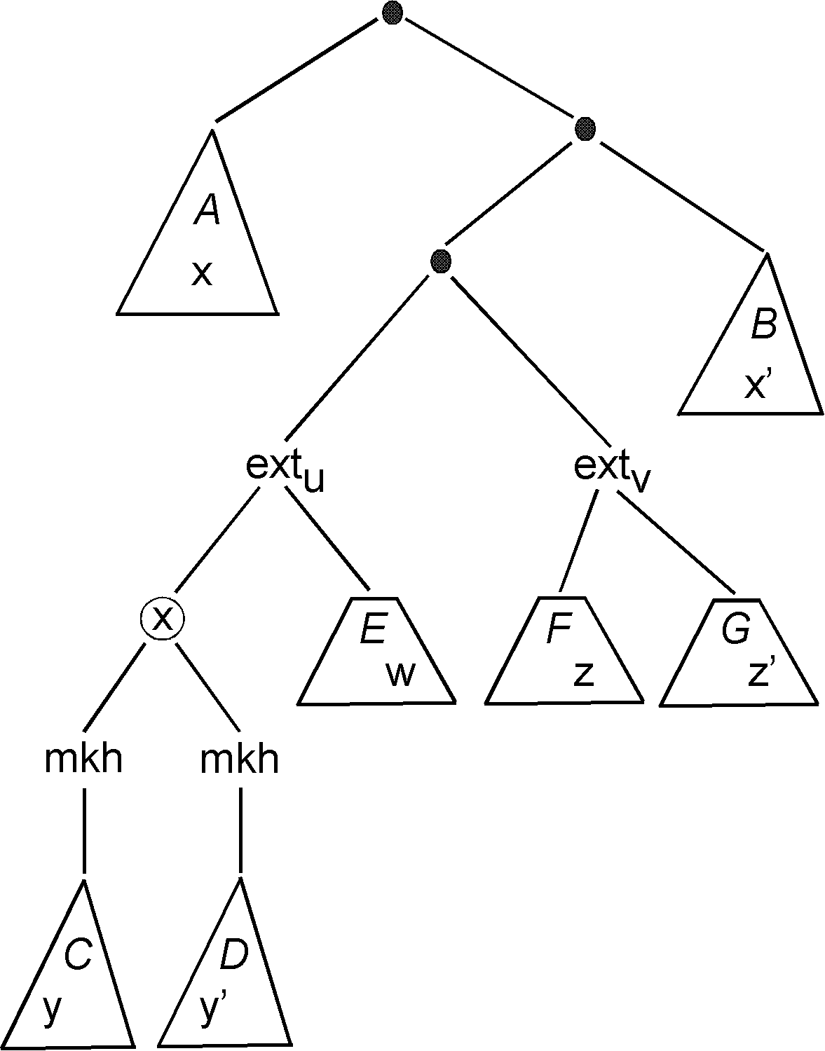
Figure 6. Term $T$ of Example (4.10).

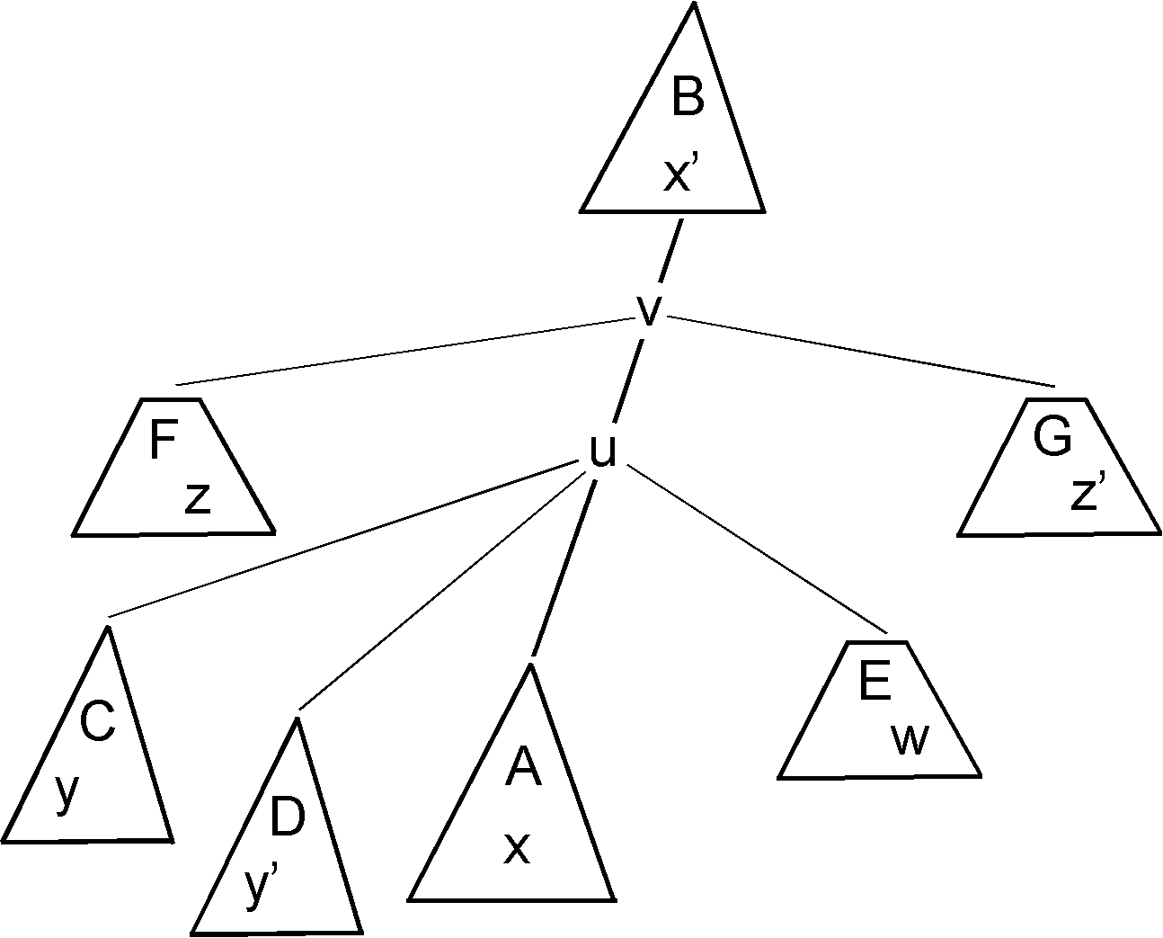
Figure 7. The OJ-tree $val(T)$ of Example (4.10).

We now illustrate this definition. Figure 6 shows a term $T$ where $A,B,C$ and $D$ are subterms of type $\boldsymbol{t}$ and $E,F$ and $G$ are subterms of type $\boldsymbol{h}$. They contain occurrences of $ext$ that define nodes $x,x^{\prime},y,y^{\prime},w,z$ and $z^{\prime}$ of $val(T)$.

The OJ-tree $val(T)$ is shown on Figure 7, where we designate by $\mathrm{A,B,\dots,G}$ the trees and hedges defined by the terms $A,B,\dots,G$. We have the following comparisons for $<$:

• $\{z,z^{\prime},u\}<v$, because $\{z,z^{\prime}\}<_{T}v$, $u<_{lex}v$ and $u\approx v$,

• $\{y,y^{\prime},w\}<u$, because $\{y,y^{\prime},w\}<_{T}u$,

• $x\leq\{u,v\}$ because $x\leq_{T}a<_{lex}\{u,v\}$ and $a\approx u\approx v$ where $a$ is the root position of $A$,

• $v<x^{\prime}$ if and only if $x^{\prime}$ is on $X$, the axis of $\mathrm{B}$, because in this case, $v\approx x^{\prime}$ and otherwise $v$ and $x^{\prime}$ are incomparable with respect to $\leq$; in all cases we have $v<_{lex}x^{\prime}$.

For $\sqsubset$ we have: $z\sqsubset y\sqsubset y^{\prime}\sqsubset x\sqsubset w\sqsubset u\sqsubset z^{\prime}\sqsubset v$ and $x^{\prime}\sqsubset z$ if $x^{\prime}$ is to the left of $X$ ; otherwise $v\sqsubset x^{\prime}$. All inequalities for $<$ yield the corresponding inequalities for $\sqsubset$. We now compare $z,y,y^{\prime},x,w,z^{\prime}$ that are pairwise incomparable for $<$.

• By Case (i) of Definition 4.5, we get $\{y,y^{\prime}\}\sqsubset w,y\sqsubset y^{\prime}$ and $z\sqsubset z^{\prime}.$

• By Case (ii), we get $x\sqsubset w,\{x,w\}\prec z^{\prime}$ and $\{y,y^{\prime}\}\prec w$.

• By Case(iii) we get $\{z,y,y^{\prime}\}\prec x$ and $z\prec\{y,y^{\prime}\}.$

Finally, if $x^{\prime}$ is to the left of $X$, then Case (iii) gives $x^{\prime}\sqsubset z,$ and if it to its right, then Case (ii) gives $z\sqsubset x^{\prime}$.

Theorem 21.

The following properties of an OJ-tree $J$ are equivalent :

1. $J$ is regular,

2. $J$ is described by a regular SOJ-scheme,

3. $J$ is MS definable.

Proof 4.7.

The proof is similar to that of Theorem 9. We only indicate some differences.

1. $\!\!\Longrightarrow$(3): Follows from Proposition 19.

2. $\!\!\Longrightarrow$(1): As observed in Definition 4.5 (cf. the claim), the mapping $\alpha$ that transforms the relational structure $\left\lfloor t\right\rfloor$ for $t$ in $T^{\infty}(F^{{}^{\prime\prime}})_{\boldsymbol{t}}$ into the OJ-tree $(N,\leq,\sqsubseteq)=\mathit{fgs}(val(t))$ is an MS-transduction. Let $J=(N,\leq,\sqsubseteq)$ be an MS definable OJ-tree. It is, up to isomorphism, the unique model of an MS sentence $\beta$. The set of terms $t$ in $T^{\infty}(F^{\prime\prime})_{\boldsymbol{t}}$ such that $\alpha(\left\lfloor t\right\rfloor)\models\beta$ is thus MS definable, hence, it contains a regular term. This term denotes $J$, hence $J$ is regular.

As in Corollaries 10 and 14, we deduce that the isomorphism problem for regular OJ-trees is decidable.

Remark 22 (An alternative notion of SOJ-tree).

We present a variant of Definition 4. If $J=(N,\leq,\sqsubseteq,A,\mathcal{U}^{-},\mathcal{U}^{+})$ is an SOJ-tree, Definition 4(c) shows that, for each $x\in N$, the partition $(\mathcal{U}^{x}\cap\mathcal{U}^{-},\mathcal{U}^{x}\cap\mathcal{U}^{+})$ of $\mathcal{U}^{x}$ is defined in a unique way from $\sqsubseteq$ and the structuring $\mathcal{U}:=\{A\}\uplus\mathcal{U}^{-}\uplus\mathcal{U}^{+}$ of $(N,\leq),$ except if $x$ has no central direction (cf. Proposition 16). This partition is useful only when $x$ is the minimal element of $A$, denoted by $\min(A)$ when it exists. To see that, we consider $J$ and another structuring of the same OJ-tree, $J^{\prime}=(N,\leq,\sqsubseteq,A,\mathcal{U}^{\prime-},\mathcal{U}^{\prime+}),$ such that $\mathcal{U}^{\prime x}=\mathcal{U}^{x}$ for each node $x\neq\min(A)$ and $\mathcal{U}^{x}\cap\mathcal{U}^{-}\neq\mathcal{U}^{\prime x}\cap\mathcal{U}^{-}$ if $x=\min(A)$. Let $K$ be a nonempty SOJ-tree. Then $K\bullet J$ is not equal to $K\bullet J^{\prime}$.

We could thus define an SOJ-tree as a tuple $S=(N,\leq,\sqsubseteq,\mathcal{U}^{\prime},\mathcal{U}_{Ax}^{-},\mathcal{U}_{Ax}^{+})$ such that $(N,\leq,\sqsubseteq)$ is an OJ-tree, $\mathcal{U}:=\mathcal{U}^{\prime}\uplus\mathcal{U}_{Ax}^{-}\uplus\mathcal{U}_{Ax}^{+}$ is a structuring of $(N,\leq)$ with axis $A$ (belonging to $\mathcal{U}^{\prime}$), $\mathcal{U}_{Ax}^{-}\uplus\mathcal{U}_{Ax}^{+}=\emptyset$ if $A$ has no minimal element, and, otherwise, $\mathcal{U}_{Ax}^{-}\uplus\mathcal{U}_{Ax}^{+}=\mathcal{U}^{\min(A)}$ and $U\sqsubset U^{\prime}$ for all $U\in\mathcal{U}_{Ax}^{-}$ and $U^{\prime}\in\mathcal{U}_{Ax}^{+}.$ Then, the structure $S$ corresponding to an SOJ-tree $(N,\leq,\sqsubseteq,A,\mathcal{U}^{-},\mathcal{U}^{+})$ is $(N,\leq,\sqsubseteq,\mathcal{U}^{\prime},\mathcal{U}_{Ax}^{-},\mathcal{U}_{Ax}^{+})$ where:

• $\mathcal{U}_{Ax}^{-}:=\mathcal{U}^{-}\cap\mathcal{U}^{\min(A)}$ and $\mathcal{U}_{Ax}^{+}:=\mathcal{U}^{+}\cap\mathcal{U}^{\min(A)}$ if $A$ has a minimal element,

• $\mathcal{U}_{Ax}^{-}:=\mathcal{U}_{Ax}^{+}:=\emptyset$ otherwise, and, in both cases,

• $\mathcal{U}^{\prime}:=\{A\}\cup\mathcal{U}^{-}\cup\mathcal{U}^{+}-(\mathcal{U}_{Ax}^{-}\cup\mathcal{U}_{Ax}^{+}).$

It is not difficult conversely to construct $(A,\mathcal{U}^{-},\mathcal{U}^{+})$ from $(N,\leq,\sqsubseteq,\mathcal{U}^{\prime},\mathcal{U}_{Ax}^{-},\mathcal{U}_{Ax}^{+})$ and to redefine the operations of Definition 4.5 in terms of the structures $S$ as above. This alternative definition of SOJ-trees contains no redundant information. However, we found the initial definition easier to handle in our logical setting.

5. Quasi-trees

Quasi-trees can be viewed intuitively as “undirected join-trees”. As in [11], we define them in terms of a ternary betweenness relation. Their use for defining rank-width is reviewed at the end of the section.

[Betweenness]

1. Let $L=(X,\leq)$ be a linear order. Its betweenness relation is the ternary relation on $X$ such that $B_{L}(x,y,z)$ holds if and only if $x<y<z$ or $z<y<x.$ It is empty if $X$ has less than 3 elements.

2. If $T$ is a tree, its betweenness relation is the ternary relation on $N_{T}$, such that $B_{T}(x,y,z)$ holds if and only if $x,y,z$ are pairwise distinct and $y$ is on the unique path between $x$ and $z$. If $R$ is a rooted tree and $T=\mathit{Und}(R)$ is the tree obtained from $R$ by forgetting its root and edge directions, then $B_{T}(x,y,z):\Longleftrightarrow x,y,z$ are pairwise distinct and, either $x<_{R}y\leq_{R}x\sqcup_{R}z$ or $z<_{R}y\leq_{R}x\sqcup_{R}z$.

3. If $B$ is a ternary relation on a set $X$, and $x,y\in X$, then $[x,y]_{B}:=\{x,y\}\cup\{z\in X\mid B(x,z,y)\}.$ This set is finite if $B=B_{T}$ for some tree $T$.

Proposition 23 (cf. [11]).

1. The betweenness relation $B$ of a linear order $(X,\leq)$ satisfies the following properties for all $x,y,z,u\in X$.

   1. $B(x,y,z)\Rightarrow x\neq y\neq z\neq x.$

   2. $B(x,y,z)\Rightarrow B(z,y,x).$

   3. $B(x,y,z)\Rightarrow\lnot B(x,z,y).$

   4. $B(x,y,z)\wedge B(y,z,u)\Rightarrow B(x,y,u)\wedge B(x,z,u).$

   5. $B(x,y,z)\wedge B(x,u,y)\Rightarrow B(x,u,z)\wedge B(u,y,z).$

   6. $B(x,y,z)\wedge B(x,u,z)\Rightarrow$ $y=u\vee[B(x,u,y)\wedge B(u,y,z)]\vee[B(x,y,u)\wedge B(y,u,z)].$

   7. $x\neq y\neq z\neq x\Rightarrow B(x,y,z)\vee B(x,z,y)\vee B(y,x,z).$

2. The betweenness relation $B$ of a tree $T$ satisfies the properties A1-A6 for all $x,y,z,u$ in $N_{T}$ together with the following weakening of A7’:

   1. $x\neq y\neq z\neq x\Rightarrow\begin{array}[t]{l}B(x,y,z)\vee B(x,z,y)\vee B(y,x,z)\,\vee\\ \exists w.(B(x,w,y)\wedge B(y,w,z)\wedge B(x,w,z))\end{array}.$

Proposition 24.

Let $B$ be a ternary relation on a set $X$ that satisfies properties A1-A7’ for all $x,y,z,u$ in $X$. Let $a$ and $b$ be distinct elements of $X$. There is a unique linear order $L=(X,\leq)$ such that $a<b$ and $B_{L}=B$. It is quantifier-free definable in the logical structure $(X,B,a,b).$

Proof 5.1.

Let $X,B,a,b$ be as in the statement. Let us enumerate $X$ as $x_{1}=a$, $x_{2}=b$, $x_{3},\dots,x_{n},\dots$ Let $X_{n}:=\{x_{1},\dots,x_{n}\}$ for $n\geq 3$. Observe that $B\upharpoonright X_{n}$ satisfies properties A1-A7’. We prove by induction on $n$ the existence and unicity of a linear order $L_{n}=(X_{n},\leq)$ such that $a<b$ and $B_{L_{n}}=B\upharpoonright X_{n}$.

• Basis: $n=3.$ The conclusion follows from A7’.

• Induction case: We assume the conclusion true for $n$.

  Claim 25.

  If $B(x_{i},x_{n+1},x_{j})$ holds for some $i<j\leq n$, then, there is a unique pair $k,l$ such that $k<l\leq n$, $B(x_{k},x_{n+1},x_{l})$ holds and $[x_{k},x_{l}]_{L}\cap X_{n+1}=\{x_{k},x_{n+1},x_{l}\}.$

  Proof 5.2.

  Assume that $x_{m}\in[x_{i},x_{j}]_{L}\cap X_{n+1}-\{x_{i},x_{n+1},x_{j}\},$ which implies $m\leq n$. Then, by A6, we have $B(x_{i},x_{n+1},x_{m})$ or $B(x_{m},x_{n+1},x_{j})$ and we can repeat the argument with $(x_{i},x_{m})$ or $(x_{m},x_{j})$ instead of $(i,j)$. Furthermore, the considered set, $[x_{i},x_{m}]_{L}\cap X_{n+1}$ or $[x_{m},x_{j}]_{L}\cap X_{n+1}$ has less elements than $[x_{i},x_{j}]_{L}\cap X_{n+1}.$Hence, we must obtain $k,l$ such that $[x_{k},x_{l}]_{L}\cap X_{n+1}=\{x_{k},x_{n+1},x_{l}\}$ as desired.

  In this case, there is a unique way to extend $L_{n}$ into $L_{n+1}$: we put $x_{n+1}$ between $x_{k}$ and $x_{l}.$ There is another case.

  Claim 26.

  If $B(x_{i},x_{n+1},x_{j})$ holds for no $i<j\leq n$, then there is a unique $k$ such that $k\leq n$, $B(x_{l},x_{k},x_{n+1})$ holds for some $l\leq n$, and $[x_{k},x_{n+1}]_{L}\cap X_{n+1}=\{x_{k},x_{n+1}\}.$ The element $x_{k}$ is extremal in $L_{n}$, that is, either maximal or minimal. ∎

  The proof is similar. In this case, there is a unique way to extend $L_{n}$ into $L_{n+1}$: we put $x_{n+1}$ after $x_{k}$ if it is maximal in $L_{n}$ or before it if it is minimal. By taking the union of all orders $L_{n}$, we get the desired and unique linear order on $X$, that we will denote by $\leq_{a,b}.$ We now define it by a first-order formula.

  We first observe a particularly simple case. If there are no $u,v\in X$ such that $B(u,b,v)$ holds, we have $x\leq_{a,b}y\Longleftrightarrow$ $x=y\vee y=b\vee B(x,y,b))$. A similar description can be given if there are no $u,v$ such that $B(u,a,v)$ holds. From $(X,B,a,b)$ as in the statement, we define the following binary relation:

  $$Z(x,y):\Longleftrightarrow x\neq y\wedge{}\\ [(B(x,a,b)\wedge\lnot B(y,x,a))\vee(x=a\wedge\lnot B(y,a,b))\vee(B(a,x,b)\wedge\lnot B(y,x,b))\vee{}\\ \qquad(x=b\wedge B(a,b,y))\vee(B(a,b,x)\wedge B(b,x,y))].$$

  It is easy to see that $x<_{a,b}y$ implies $Z(x,y)$. In particular, $Z(a,b)$ holds by the clause $x=a\wedge\lnot B(y,a,b)$ with $y=b$. For the converse, assume that $Z(x,y)$ holds and $x<_{a,b}y$ does not. Then, we have $y<_{a,b}x$ because $\leq_{a,b}$ is a linear order. By looking at the different relative positions of $x,y,a$ and $b$, we get a contradiction. Hence $x\leq_{a,b}y$ if and only if $x=y\vee Z(x,y)$, which is expressed by a quantifier-free formula $\xi(a,b,x,y).$

Remark 27.

If there are no $u,v\in X$ such that $B(u,b,v)$ holds, then:

$$Z(x,y)\Longleftrightarrow x\neq y\wedge[(B(x,a,b)\wedge\lnot B(y,x,a))\vee(x=a\wedge\lnot B(y,a,b))\vee$$

$$(B(a,x,b)\wedge\lnot B(y,x,b))]$$

which is equivalent to $y=b\vee B(x,y,b))$ as one can (painfully) check by using axioms A1-A7’.

[Quasi-trees]

1. A quasi-tree is a structure $S=(N,B)$ such that $B$ is a ternary relation on $N$, called the set of nodes, that satisfies conditions A1-A7 (a definition from [11]). To avoid uninteresting special cases, we also require that $N$ has at least 3 nodes.

   Lemma 11 of [11] shows that in a quasi-tree, the four cases of the conclusion of A7 are exclusive and that, in the fourth one, there is a unique node $w$ satisfying $B(x,w,y)\wedge B(y,w,z)\wedge B(x,w,z)$, which we denote by $M_{S}(x,y,z)$.

   A leaf (of $S)$ is a node $z$ such that $B(x,z,y)$ holds for no $x,y.$ A line is set of nodes $L$ such that $[x,y]_{B}\subseteq L$ if $x,y\in L$ and $(L,B\upharpoonright L)$ satisfies A7’. We say that $S$ is discrete if each set $[x,y]_{B}$ is finite. A quasi-tree $S=(N,B)$ is a subquasi-tree of a quasi-tree $S^{\prime}=(N^{\prime},B^{\prime})$, which we denote by $S\subseteq S^{\prime}$, if $N\subseteq N^{\prime}$ and $B=B^{\prime}\upharpoonright N$. This condition implies that $M_{S}=M_{S^{\prime}}\upharpoonright N$.

2. From a join-tree $J=(N,\leq),$ we define a ternary relation $B_{J}$ on $N$ by:

   $$B_{J}(x,y,z):\Longleftrightarrow x\neq y\neq z\neq x (x<y\leq x\sqcup z)\vee(z<y\leq x\sqcup z)$$ and .

Proposition 28.

1. The structure $\mathit{qt}(J):=(N,B_{J})$ associated with a join-tree $J=(N,\leq)$ having at least 3 nodes is a quasi-tree. Every line of $J$ is a line of $\mathit{qt}(J)$. If $J$ is a subjoin-tree of $J^{\prime}$, then $\mathit{qt}(J)$ is a subquasi-tree of $\mathit{qt}(J^{\prime})$.

2. Every quasi-tree $S$ is $\mathit{qt}(J)$ for some join-tree $J$.

3. A quasi-tree is discrete if and only if it is $\mathit{qt}(J)$ for some rooted tree $J$.

Proof 5.3.

1. Let $J=(N,\leq)$ be a join-tree with at least 3 nodes.

   If it is finite, then it is $(N_{T},\leq_{T})$ for a finite rooted tree $T$, and $\mathit{qt}(J)$ is a finite quasi-tree by Proposition 23(b).

   Otherwise consider distinct elements $x,y,z,u$ of $N$. We want to prove that they satisfy A1-A7. There is a set $N^{\prime}\subseteq N$ of cardinality at most 7 that contains $x,y,z,u$ and is closed under $\sqcup$. Then $J^{\prime}=(N^{\prime},\leq\upharpoonright N^{\prime})$ is a finite join-tree, $J^{\prime}\subseteq J$ and $\mathit{qt}(J^{\prime})=(N^{\prime},B_{J}\upharpoonright N^{\prime})$ is a quasi-tree by the initial observation, so that $x,y,z,u$ satisfy A1-A7 for $B=B_{J^{\prime}}$ hence, also for $B_{J}$. (The node $w$ that may be necessary to satisfy A7 may have to be chosen in the set $\{x\sqcup y,x\sqcup z,x\sqcup u,\dots\}$). As $x,y,z,u$ are arbitrary, A1-A7 hold for $B_{J}$ and all $x,y,z,u\in N.$ Hence, $(N,B_{J})$ is a quasi-tree.

   That every line of $J$ is a line of $\mathit{qt}(J)$ follows from the definitions. (The converse does not hold.) The assertion about subjoin-trees is also easy to prove.

2. Let $S=(N,B)$ be a quasi-tree and $r$ be any element of $N$. We define $x\leq_{r}y:\Longleftrightarrow y\in[x,r]_{B}$. Then $(N,\leq_{r})$ is a join-tree $J$ with root $r$ and $S=\mathit{qt}(J)$ by Lemma 14 of [11].

3. A quasi-tree $S=\mathit{qt}(J)$ is discrete if $J$ is rooted tree. Conversely, if $S$ is a discrete quasi-tree, then $S=\mathit{qt}(T)$ for some tree $T$ by Proposition 17 of [11]. By choosing any node as a root, one makes $T$ into a rooted tree, and its betweenness relation is that of $T$.

We say that a quasi-tree $S$ is described by an SJ-scheme if this scheme describes a join-tree $J$ such that $\mathit{qt}(J)=S$. It is regular if it is $\mathit{qt}(J)$ for some regular join-tree $J$.

Proposition 29.

A quasi-tree is MS_fin-definable if it is described by a regular SJ-scheme.

Proof 5.4.

We first prove a technical result.

Claim 30.

There exists a first-order formula $\mu(L,a,b,u,v)$ such that, for every join-tree $J=(N,\leq),$ if $S=\mathit{qt}(J)=(N,B),$ then there is a subset $L$ of $N$ and elements $a,b$ of $N$ such that, for every $u,v\in N$, $(N,B)\models\mu(L,a,b,u,v)$ if and only if $u\leq v$.

Proof 5.5 (Proof of the claim).

The formula $\mu(L,a,b,u,v)$ will be defined as $u=v\vee\mu_{1}(L,a,b,u,v)\vee\mu_{2}(L,a,b,u,v)$ so as to handle two exclusive cases relative to $J=(N,\leq)$.

• Case $J=(N,\leq)$ has a root $r$. Then, $u<v$ if and only if $v=r$ or $B(u,v,r)$. Hence, we define $\mu_{1}(L,a,b,u,v)$ as $L=\emptyset\wedge a=b\wedge(v=b\vee B(u,v,b)).$

• Case $J$ has no root. It has a line $L$ that is upwards closed, i.e., such that $y\in L$ if $x\leq y$ and $x\in L$. This line has no maximal element (otherwise its maximal element would be a root of $J$) and is infinite. Moreover, for every $u\in N$, we have $u<x$ for some $x\in L$ (to prove that, consider $u\sqcup y$ where $y$ is any element of $L$). For all $u,v\in N$ we have:

  $$u<v\Longleftrightarrow\exists x,y\in L[x<y\wedge B(u,v,x)\wedge B(v,x,y)].$$

  If $u<v$ we have $u<v<x<y$ for some $x,y$ in $L$. Hence, we have $B(u,v,x)\wedge B(v,x,y).$ Assume for the converse that $x<y\wedge B(u,v,x)\wedge B(v,x,y)$ for some $x,y$ in $L$. We first prove that $u,v<x$. Since $B=B_{J}$, $B(v,x,y)\Longleftrightarrow$ $v<x\leq v\sqcup y\vee y<x\leq y\sqcup v$. As $x<y$, we must have $v<x$. Axiom A4 gives $B(u,x,y),$ from which we get similarly $u<x$. From $B(u,v,x)$ we get $u<v\leq u\sqcup x$ or $x<v\leq x\sqcup v$. As $v<x$, we have $u<v$. Let $a,b\in L$ such that $a<b$. Proposition 24 is applicable to $(L,B\upharpoonright L)$ that satisfies Conditions A1-A7’. Hence the quantifier-free formula $\xi(a,b,x,y)$ defines $x<_{a,b}y$ for $x,y\in L$. We define $\mu_{2}(L,a,b,u,v)$ as $\exists x,y\in L[a,b\in L\wedge\xi(a,b,x,y)\wedge B(u,v,x)\wedge B(v,x,y)].$

We now complete the proof. If $J=(N,\leq)$ has a root $r$, we choose $L=\emptyset\wedge a=b=r$, $\mu_{2}(L,a,b,u,v)$ is false and $\mu_{1}(L,a,b,u,v)$ is equivalent to $u<v$. If $J$ has no root, we let $L$ be an upwards closed line, and $a,b\in L$ such that $a<b$. Then $\mu_{1}(L,a,b,u,v)$ is false and $\mu_{2}(L,a,b,u,v)$ is equivalent to $u<v$.

We let $\mu^{\prime}(L,a,b,u,v)$ be $u=v\vee\mu(L,a,b,u,v)$. For proving the main assertion, we let $S=\mathit{qt}(J)$ be a quasi-tree defined from a regular join-tree $J$ and $\psi$ be the MS_fin sentence expressing that a structure $(N,\leq)$ is a join-tree isomorphic to $J$; this sentence exists by Theorem 13. Let $\varphi$ be the MS_fin sentence expressing that a structure $(D,B)$ is a quasi-tree that satisfies $\exists L,a,b(\psi^{\prime}\wedge$“$B$ is the betweenness relation of the order relation $\leq$ defined by $\mu^{\prime}$”$)$ where $\psi^{\prime}$ is obtained from $\psi$ by replacing each atomic formula $x\leq y$ by $\mu^{\prime}(L,a,b,x,y)$.

Then $\mathit{qt}(J)$ satisfies $\varphi$ by the claim. If conversely, $(D,B)$ satisfies $\varphi$ for some $L,a$ and $b$, then $(D,\leq)$ is a join-tree $J^{\prime}$, where $x\leq y$ is defined in $(D,B)$ by $\mu^{\prime}(L,a,b,x,y)$ (because $\psi^{\prime}$ holds), $(D,B)=\mathit{qt}(J^{\prime})$ (because $B$ is the betweenness relation of $\leq$) and $J^{\prime}\simeq J$ (because of $\psi^{\prime}$). Hence, $(D,B)\simeq\mathit{qt}(J)$. Hence $\mathit{qt}(J)$ is characterized by $\varphi$ up to isomorphism.

The next theorem establishes a converse. As algebra for quasi-trees, we take the algebra $\mathbb{SJT}$ of join-trees together with the (external) operation $\mathit{qt}$ (similar to $\mathit{fgs}$) that makes a join-tree into a quasi-tree.

Theorem 31.

The following properties of a quasi-tree $S$ are equivalent:

1. $S$ is regular,

2. $S$ is described by a regular SJ-scheme,

3. $S$ is MS_fin definable.

Furthermore, the isomorphism problem of regular quasi-trees is decidable.

Proof 5.6.

1. $\!\!\Rightarrow$(2): The proof is similar to that of Theorem 9.

2. $\!\!\Rightarrow$(3): By Proposition 29.

3. $\!\!\Rightarrow$(1): The mapping $\alpha$ that transforms the relational structure $\left\lfloor t\right\rfloor$ for $t$ in $T^{\infty}(F^{\prime})_{\boldsymbol{t}}$ into the quasi-tree $S=\mathit{qt}(\mathit{fgs}(val(t)))$ is an MS-transduction by Definitions 4.5 (cf. the claim) and 27(b). The proof continues as in Theorem 9.

The decidability of the isomorphism problem is as in Corollary 10.

We make these results more precise for subcubic quasi-trees: they are useful for defining the rank-width of countable graphs, as we will recall.

[Directions]

Let $S=(N,B)$ be a quasi-tree and $x$ a node of $S$.

1. We say that $y,z\in N-\{x\}$ are the same direction relative to $x$ (or of $x$) if, either $y=z$ or $B(y,z,x)$ or $B(z,y,x)$ or $B(y,u,x)\wedge B(z,u,x)$ for some node $u$ (a definition from [11]). Equivalently, $y\sqcup_{x}z<_{x}x$ ($<_{x}$ is as in Proposition 28(2)). Hence, if $B(y,x,z)$ holds, then $y$ and $z$ are in different directions relative to $x$. This relation is an equivalence, denoted by $y\sim_{x}z$, and its classes are the directions of $x$.

2. The degree of $x$ is the number of classes of $\sim_{x}$. A node has degree 1 if and only if it is a leaf. We say that $S$ is subcubic if its nodes have degree at most 3. If $S=\mathit{qt}(T)$ for a tree $T$, then a direction of $x$ is associated with each neighbour $y$ of $x$ and is the set of nodes of the connected component of $T-\{x\}$ that contains $y$.

3. If $S=\mathit{qt}(J)$ for a join tree $J=(N,\leq)$, then, the directions of $x$ in $S$ are those of $x$ in $J$ together with the set $N-\mathopen{]}-\infty,x]$ if it is not empty. It follows that $S$ is subcubic if $J$ is a BJ-tree.

Lemma 32.

Every subcubic quasi-tree is $\mathit{qt}(\mathit{fgs}(J))$ for some SBJ-tree $J$.

Proof 5.7.

Let $S$ be a subcubic quasi-tree. Then $S=\mathit{qt}(J)$ for some join-tree $J$. We choose a maximal line $L$ of $J$ and $a,b\in L$ such that $a<b.$ By Proposition 29, the partial order $\leq$ of $J$ is defined by $\mu^{\prime}(L,a,b,x,y)$. The method of Proposition 2 with $U_{0}:=L$, gives structuring $K$ of $J$, making it into an SBJ-tree as defined in Definition 3.2.

Theorem 33.

The following properties of a subcubic quasi-tree $S$ are equivalent :

1. $S$ is regular,

2. $S$ is described by a regular SBJ-scheme,

3. $S$ is MS definable.

Proof 5.8.

By Lemma 32 and Proposition 8, every subcubic quasi-tree $S$ is $\mathit{qt}(\mathit{fgs}(val(t)))$ for some term $t\in T^{\infty}(F)$.

Property (1) means that $S=\mathit{qt}(\mathit{fgs}(val(t)))$ for some regular term in $T^{\infty}(F^{\prime})_{\boldsymbol{t}}$. Let (1’) mean that $S=\mathit{qt}(\mathit{fgs}(val(t)))$ for some regular term in $T^{\infty}(F)$. Then (1’)$\Longrightarrow$(2) by the similar implication in Theorem 9.

(2)$\Longrightarrow$(3) by the similar implication in Theorem 9 and the observation that, in a quasi-tree $S$, the SBJ-trees $J$ such that $S=\mathit{qt}(\mathit{fgs}(J))$ can be specified by MS formulas in terms of a 5-tuple $(A,N_{0},N_{1},a,b)$ satisfying the formula $\varphi^{\prime}(A,N_{0},N_{1},a,b)$ of the proof of Proposition 29.

(3)$\Longrightarrow$(1’) by the observation that the mapping $\alpha$ that transforms the relational structure $\left\lfloor t\right\rfloor$ for $t$ in $T^{\infty}(F)$ into the subcubic quasi-tree $\mathit{qt}(\mathit{fgs}(val(t)))$ is an MS-transduction. The proof goes then as in Theorem 9.

The implication (1’)$\Longrightarrow$(1) is trivial and (1) implies that $S$ is MS_fin definable by Proposition 29. But a term $t\in T^{\infty}(F)$ that defines $S$ is MS definable, and the relational structure representing a term has an MS definable linear order. It follows that $S$ has an MS definable linear order, hence that $S$ is MS definable by the facts recalled in Section 2.

We now review the use of quasi-trees for rank-width [11], a width measure first defined and investigated in [21] and [22] for finite graphs.

[Rank-width for countable graphs]

We consider finite or countable, loop-free, undirected graphs without parallel edges. The adjacency matrix of such a graph $G$ is $M_{G}:V_{G}\times V_{G}\rightarrow\{0,1\}$ with $M_{G}[x,y]=1$ if and only if $x$ and $y$ are adjacent. If $U$ and $W$ are disjoint sets of vertices, $M_{G}[U,W]$ is the matrix that is the restriction of $M_{G}$ to $U\times W$. The rank (over $GF(2)$) of $M_{G}[U,W]$ is the maximum cardinality of an independent set of rows (equivalently, of columns) and is denoted by $rk(M_{G}[U,W]);$ it belongs to $\mathbb{N}\cup\{\omega\}$. We take $rk(M_{G}[\emptyset,W])=rk(M_{G}[U,\emptyset]):=0.$ If $X\uplus Y$ is infinite, then $rk(M_{G}[X,Y])=\sup\{rk(M_{G}[U,W])\mid U\subseteq X,W\subseteq Y$ and, $U$ and $W$ are finite}.

A discrete layout of a graph $G$ is an unrooted tree $T$ of maximal degree 3 whose set of leaves is $V_{G}$. Its rank is the least upper-bound of the ranks $rk(M_{G}[X\cap V_{G},X^{c}\cap V_{G}])$ such that $X$ and $X^{c}:=N_{T}-X$ are the two connected components of $T$ minus one edge. The discrete rank-width of $G,$ denoted by $rwd^{dis}(G),$ is the smallest rank of a discrete layout. If $G$ is finite, this value is the rank-width defined in [21]. By using for countable graphs $G$ quasi-trees with nodes of maximal degree 3 instead of trees, one obtains their rank-with $rwd(G)$ (cf. [11] for details). We have $rwd(G)\leq rwd^{dis}(G)$. The notation $G\subseteq_{i}H$ means that $G$ is an induced subgraph of $H$.

Theorem 34 (cf. [11]).

For every graph $G$:

1. if $H\subseteq_{i}G$, then $rwd(H)\leq rwd(G)$ and $rwd^{dis}(H)\leq rwd^{dis}(G)$,

2. Compactness: $rwd(G)=\mathrm{Sup}\{rwd(H)\mid H\subseteq_{i}G$ and $H$ is finite$\},$

3. Compactness with gap : $rwd^{dis}(G)\leq 2\cdot\mathrm{Sup}\{rwd(H)\mid H\subseteq_{i}G$ and $H$ is finite$\}.$

The gap function in (3) is $n\mapsto 2n$, showing a weak form of compactness. The proof of (2) uses Koenig’s Lemma, and consists in taking $G$ as the union of an increasing sequence of finite induced subgraphs. The desired layout of $G$ is obtained from an increasing sequence of finite layouts of finite induced subgraphs where nodes are successively added. The union of these layouts is in general a quasi-tree and not a tree.

6. Conclusion

We have defined regular join-trees of different kinds and regular quasi-trees from regular terms. These terms have finitary descriptions. Other infinite terms have finitary descriptions: the algebraic ones [9] and more generally, those of Caucal’s hierarchy [5]. Such terms also yield effective (algorithmically usable) notions of join-trees and quasi-trees. It is unclear whether the corresponding isomorphism problems are decidable.

The article [7] establishes that a set of arrangements is recognizable if and only if it is MS definable. One might wish to extend this result to sets of join-trees and quasi-trees. An appropriate notion of recognizability must be defined.

References

- [1] S. Bloom and Z.Ésik. Deciding whether the frontier of a regular tree is scattered. Fundam. Inform. 55 (2003) 1-21.
- [2] S. Bloom and Z.Ésik. The equational theory of regular words. Inf. Comput. 197 (2005) 55-89.
- [3] S. Bloom and Z.Ésik. Algebraic ordinals. Fundam. Inform. 99 (2010) 383-407.
- [4] S. Bloom and Z.Ésik. Algebraic linear orderings. Int. J. Found. Comput. Sci. 22 (2011) 491-515.
- [5] A. Blumensath, T. Colcombet and C.Löding. Logical theories and compatible operations, in Logic and Automata: History and perspectives, J. Flum et al. eds, Amsterdam University Press, 2008, pp. 73-106.
- [6] A. Blumensath and B. Courcelle. Monadic second-order definable graph orderings. Logical Methods in Computer Science 10 (2014), issue 1.
- [7] O. Carton, T. Colcombet and G. Puppis. Regular languages of words over countable linear orderings, 2015, submitted, see https://arxiv.org/abs/1702.05342, Extended abstract in Proccedings of ICALP, Lecture Notes in Computer Science 6756 (2011) 125-136.
- [8] B. Courcelle. Frontiers of infinite trees. ITA (Informatique Théorique et Applications) 12 (1978) 317-339 (former name of the journal: RAIRO Informatique Théorique).
- [9] B. Courcelle. Fundamental properties of infinite trees. Theor. Comput. Sci. 25 (1983) 95-169.
- [10] B. Courcelle. Clique-width of countable graphs: a compactness property. Discrete Mathematics 276 (2004) 127-148.
- [11] B. Courcelle. Several notions of rank-width for countable graphs, J. Comb. Theory, Ser. B 123 (2017) 186-214.
- [12] B. Courcelle. Regularity equals monadic second-order definability for quasi-trees, in Fields of Logic and Computation II, Lec. Notes Comput. Sci. 9300 (2015) 129-141.
- [13] B. Courcelle and C. Delhommé. The modular decomposition of countable graphs. Definition and construction in monadic second-order logic. Theor. Comput. Sci. 394 (2008) 1-38.
- [14] B. Courcelle and J. Engelfriet. Graph structure and monadic second-order logic, a language theoretic approach, Cambridge University Press, 2012.
- [15] Z. Ésik. An undecidable property of context-free linear orders. Inf. Process. Lett. 111 (2011) 107-109.
- [16] R. Fraïssé, Theory of relations, Studies in Logic, Volume 145, North-Holland, 2000.
- [17] J. Goguen, J. Thatcher, E. Wagner and J. Wright. Initial algebra semantics and continuous algebras. J. ACM 24 (1977) 68-95.
- [18] S. Heilbrunner. An algorithm for the solution of fixed-point equations for infinite words. ITA 14 (1980) 131-141.
- [19] I. Kriz and R. Thomas. Clique-sums, tree-decompositions and compactness. Discrete Mathematics 81 (1990) 177-185.
- [20] S. Lifsches and S. Shelah. Uniformization, choice functions and well orders in the class of trees, Journal of Symbolic Logic 61 (1996) 1206-1227.
- [21] S. Oum. Rank-width and vertex-minors, J. Comb. Theory, Ser. B 95 (2005) 79-100.
- [22] S. Oum and P. Seymour. Approximating clique-width and branch-width. J. Comb. Theory, Ser. B 96 (2006) 514-528.
- [23] W. Thomas. On frontiers of regular trees, ITA 20 (1986) 371-381.
- [24] W. Thomas. Automata on infinite objects, in Handbook of Theoretical Computer Science, Volume B, Elsevier 1990, pp. 133-192.
- [25] M. Rabin. Decidability of second-order theories and automata on infinite trees, Transactions of the American Mathematical Society, 141 (1969) 1-35.
- [26] J. Sakarovitch. Elements of Automata Theory, Cambridge University Press, 2009.