Electrical Addressing and Temporal Tweezing of Localized Pulses
in Passively Mode-Locked Semiconductor Lasers

Abstract

We show that the pumping current is a convenient parameter for manipulating the temporal Localized Structures (LSs), also called localized pulses, found in passively mode-locked Vertical-Cavity Surface-Emitting Lasers. While short electrical pulses can be used for writing and erasing individual LSs, we demonstrate that a current modulation introduces a temporally evolving parameter landscape allowing to control the position and the dynamics of LSs. We show that the localized pulses drifting speed in this landscape depends almost exclusively on the local parameter value instead of depending on the landscape gradient, as shown in quasi-instantaneous media. This experimental observation is theoretically explained by the causal response time of the semiconductor carriers that occurs on an finite timescale and breaks the parity invariance along the cavity, thus leading to a new paradigm for temporal tweezing of localized pulses. Different modulation waveforms are applied for describing exhaustively this paradigm. Starting from a generic model of passive mode-locking based upon delay differential equations, we deduce the effective equations of motion for these LSs in a time-dependent current landscape.

I introduction

Localized structures (LSs) in optical resonators have attracted much interest in the last twenty years. While LS are ubiquitous in nature WKR-PRL-84 ; MFS-PRA-87 ; NAD-PSS-92 ; UMS-NAT-96 ; AP-PLA-01 and their investigation conveys an intrinsic fundamental appeal, optical LSs are very attractive also for applications. Because they can be individually addressed and manipulated, LSs can be used as elementary bits of information for all-optical information processing RK-OS-88 ; TML-PRL-94 ; FS-PRL-96 ; 1172836 . Localized structures appear in nonlinear systems having a large aspect-ratio and they rely on the coexistence between a pattern (pulsed) state with a stable homogeneous (stationary) one, though different scenarios exist as well. In the weak dissipative limit, LSs can be interpreted as dissipative solitons TF-JPF-88 ; FT-PRL-90 .

Localized structures have been observed in optical resonators both in their transverse section and along their longitudinal dimension. In the former case they appear as localized beams of light (spatial LSs) and they have been successfully implemented in broad-area semiconductor Vertical-Cavity Surface-Emitting Lasers (VCSELs) BTB-NAT-02 ; GBG-PRL-08 ; TAF-PRL-08 ; EGB-APB-10 . In the latter case they appear as localized temporal light pulses (temporal LSs). In the time domain the large aspect-ratio condition requires the resonator round-trip to be much larger than any internal timescales of the system, a condition which has been implemented, for example, in Kerr cavities LCK-NAP-10 ; HBJ-NAP-14 .

Another remarkable property of LSs is related to their plasticity. Because of translational invariance, LSs exhibit a Goldstone mode FS-PRL-96 ; MFH-PRE-02 which is excited by any inhomogeneous parameter variation, thus inducing their motion. Because the velocity, instead of the acceleration, is proportional to the parameter variations, the latter is interpreted as an Aristotelian force which allows for LS reconfiguration and drift FGB-APL-06 ; PBC-APL-08 ; JEC-NAC-15 .

Semiconductor gain media, which typically exhibit nanosecond response timescales (owing to the recombination rate of carriers), are promising for achieving large temporal aspect-ratio condition required for temporal localization. Accordingly, temporal LSs have been recently observed in semiconductor lasers mounted in compound cavities configurations. Several regimes have been exploited to provide the dynamical ingredients leading to LS: front stabilization MGB-PRL-14 ; JAH-PRL-15 , passive mode-locking MJB-PRL-14 , excitability GJT-NC-15 ; RAF-SR-16 , and polarizations competition MJB-NAP-15 . Interesting enough, the dynamics of these systems is affected by the finite response of the carriers, i.e. their causal response, thus breaking the parity invariance along the longitudinal direction of the cavity.

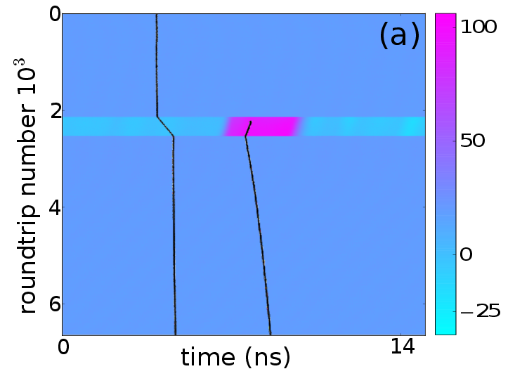
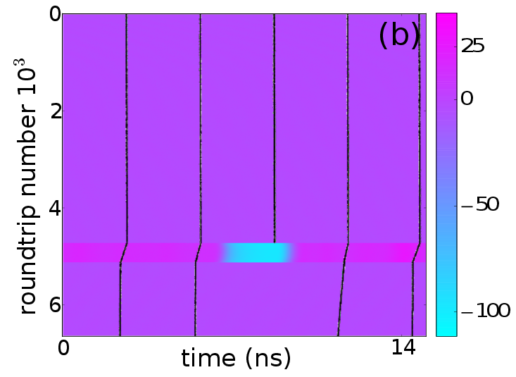
Figure 1: Spatio-temporal diagrams showing the addressing, i.e. the writing (a) and the erasing (b) of a LS, by an electrical pulse in the pumping current. The current values are represented in color scales, while optical pulses trajectories are represented by black lines. $J_{cw}=211\,$mA. The amplitude and the width of the writing pulse are $A=130\,$mA and $2.9\,$ns, respectively.

In this paper we consider an electrically-biased broad-area VCSEL coupled to a resonant saturable absorber mirror (RSAM) which leads to passive mode-locking MJB-JSTQE-15 . In the limit of cavity round-trips much longer than the gain recovery time, we have shown that mode-locked pulses may coexist with the zero intensity background. In this condition, these pulses become localized, i.e. they are temporal localized structures which can be individually addressed by a perturbation pulse MJB-PRL-14 . In the recent years, temporal LSs have been addressed all-optically by perturbation of the phase/amplitude of the injected field LCK-NAP-10 ; GJT-NC-15 . On the other hand, in electrically-biased semiconductor lasers, the pumping current can be easily modulated at several gigahertz rates, as demonstrated in opto-electronics for converting an electrical bit-stream into an optical one Freeman . Accordingly, the bias current is a convenient parameter for addressing and manipulating LSs in view of their applications. We have recently shown that, in a modulated current landscape, the resulting drifting speed of the localized pulses is not simply proportional to the gradient of the landscape, as it occurs in quasi-instantaneous media JEC-NAC-15 , but it rather depends on the local value of the parameter itself JCM-PRL-16 . This difference, which is ascribed to the lack of parity invariance described above, leads to a new paradigm for LS manipulation which will be described in details in this work.

The manuscript is organized as follows : Section II provides a detailed experimental analysis of the individual writing and erasing of LSs by using electrical pulses in the pumping current. In section III we analyze experimentally the motion and the reconfiguration of LSs in presence of a temporal parameter landscape introduced by modulating the pumping current with different kinds of waveforms. The theoretical analysis of these results is described in section IV where the Effective Equations of Motion (EEM) for multiple LSs in a parameter landscape are presented and used to explain our experimental results.

II Individual addressing of localized pulses

We consider the setup described in MJB-PRL-14 ; MJB-JSTQE-15 consisting of an electrically biased broad-area ($200\,\mu$m) VCSEL mounted in an external cavity closed by a resonant saturable absorber mirror (RSAM). Passive Mode-Locking is achieved when placing the RSAM surface in the Fourier transform plane of the VCSEL near-field profile. While this scheme leads to conventional mode-locking pulses for cavity round-trips shorter than the gain recovery time ($\tau<\tau_{g}$), we operate the system in the regime of long cavities, i.e. $\tau\gg\tau_{g}$, and for bias currents below the lasing threshold of the compound system ($J_{th}\sim 350\,$mA). In these conditions a large variety of pulsating emission states coexist, each one characterized by a different number $N$ of pulses circulating in the cavity or, when having the same value of $N$, characterized by different pulse arrangements. The number of pulses $N$ spans from zero up to a maximum $N_{max}$ which depends on the cavity length. This generalized multistability provides the dynamical ingredients for the formation of LSs. The state at which $N=N_{max}$ corresponds to the fully developed temporal pattern which is, together with the coexisting stable off solution, at the origin of the LS formation scenario. In analogy to spatial LSs CRT-C-94 ; CRT-PRL-00 , the temporal pattern is fully decomposable because any pulse of this solution can be set on or off by a perturbation pulse MJB-PRL-14 . We have fixed our cavity length to 2.25 m, corresponding to a round-trip time $\tau=15.02\,$ns, leading to $N_{max}=19$.

Writing and erasure of temporal LSs can be implemented by perturbing the system with an optical pulse injected inside the cavity, as done in LCK-NAP-10 ; GJT-NC-15 . The perturbation pulse must be sufficiently short in time for addressing a single LS. In this paper we take advantage of the fast response of semiconductor media to the pumping current modulation and we apply the addressing perturbation by adding electrical pulses to the laser bias. This parameter appears the most convenient in view of opto-electronic applications; conversion of an electrical bit stream into an optical one has been recently achieved by modulating laser current at more than 10 GHz Freeman . Unfortunately, because of the electrical characteristics of the laser package we have used, the modulation of the laser current suffers of stronger bandwidth limitations with a low frequency cut off at 0.2 MHz and a high frequency cut off at 500 MHz. Still, this frequency window is wide enough to allow for a proof-of-principle demonstration of LSs’ addressing operation.

The system is initially prepared in the multistable parameter region where LSs exist, and the amplitude of the addressing current pulse is chosen to be sufficiently large to bring the system locally above threshold, i.e. into the parameter region where only the temporal pattern solution is stable. If the electrical pulse is sufficiently short, a single LS will be excited and it will remain after the perturbation is removed. Similarly, a single localized structure can be erased by using a negative bias current pulse which brings the system in the parameter region where only the off solution is stable. In our case, the electrical pulse has a rectangular shape with a duration of $2.9\,$ns and it is applied synchronously with the cavity round trip-time for 390 consecutive round-trips. These two characteristics of the electrical pulses are imposed by the performances of the pulse generator used in burst mode. Unfortunately, it was not possible to obtain shorter burst of pulses, nor shorter pulses.

In order to follow the evolution of LSs inside the cavity we depict the laser intensity output using the so-called space-time diagrams, where the time trace is transformed into a two-dimensional representation with a folding parameter equal to the pulse repetition period $T$. Accordingly, the round-trip number $n$ becomes a pseudo-time variable while the pseudo-space variable corresponds to the timing of the pulse modulo $T$. This representation is similar to the one used to display the evolution of pulses along optical fibers where fast and slow timescales are well separated and it has been proposed also for delayed systems AGL-PRA-92 , yielding, in some cases, to a direct equivalence with the Ginzburg-Landau equation GP-PRL-96 .

The bias current evolution is represented on the space time diagram using a color code, while the trajectory of the LS is represented by a black trace. In Fig. 1a) we illustrate a writing operation using a current pulse applied between round-trip $n_{1}=2136$ and round-trip $n_{2}=2526$. We choose an initial condition where a single LS is present inside the cavity. The perturbation pulse excites a second LS which remains after the perturbation is removed. Figure 1a) is an example of a writing operation starting from a particular initial condition. Other initial conditions can be chosen with similar results, provided that the addressing pulse is separated in time from the preexisting LSs of at least $1\,$ns. On the other hand, we notice that, after the electrical pulse is removed, the written LS drifts to the right, thus disclosing the existence of a repulsive force exerted by the first LS on the written one. This repulsive interaction is asymmetric since the leftmost LS pushes the rightmost LS but not vice-versa. The latency in the writing process and the repulsive interaction are explained by the gain depletion induced by a LS and will be detailled in Section IV. The gain recovery process follows an exponential law with a typical time constant of $\Gamma^{-1}\sim 1\,$ns. Accordingly, the gain depression prevents writing two LSs in a time interval smaller than $\Gamma^{-1}\sim 1\,$ns, while the repulsive force between neighbor LS becomes negligible after $\sim 3\Gamma^{-1}$, i.e.$3\,$ns JCM-PRL-16 . These evidences indicate that, even if the intensity profile of a single temporal LS exhibits a temporal width of approximately 10 ps, the effective LS width is ultimately fixed by the underlying gain recovery process.

Incidentally one notes in Fig. 1a) that the trajectory of the preexisting LS changes when the electrical pulse is applied. This is explained by the current profile of the perturbation pulse which, around the 2.9 ns rectangular peak, adds a negative contribution to the steady bias current, thus changing the drifting speed of the preexisting LS. The influence of the pumping current landscape on the drifting speed of the LSs will be addressed in the next section.

Finally, an example of an erasing operation is shown in Fig. 1b), where the initial condition is composed of five preexisting LSs. A negative pulse of $2.9\,$ns is sent into the laser current between the round-trips $n_{1}=4710$ and $n_{2}=5100$, targeting the third LS from the left. It successfully erases the third LS which remains off after the perturbation is removed. It is worthwhile noting the reorganization of the positions of the other LSs after the erasing operation; the fourth LS starts to drift to the left, because the repulsive force exerted by the erased LS has disappeared. The asymmetrical interactions between LSs will be discussed more in details in Section IV.

III Motion of localized pulses

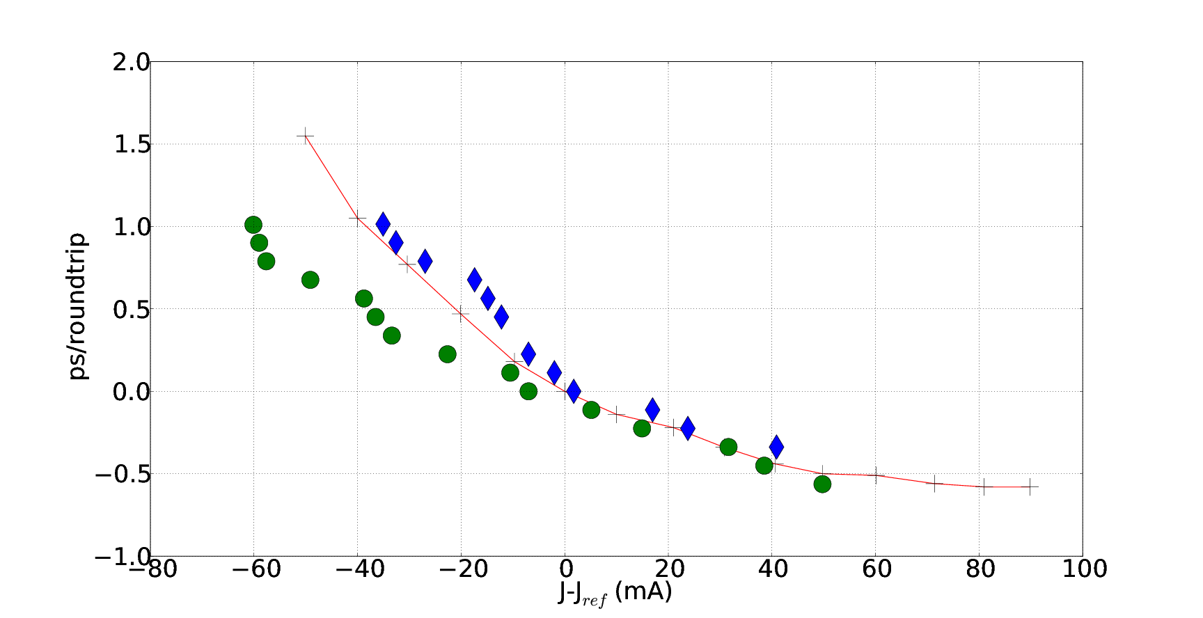
Figure 2: Drifting speed per round-trip of a LS induced by a bias current variation around a reference value ($J-J_{ref})$, $J_{ref}=226\,$mA. Bias current has been changed in different ways: (crosses connected by red line) by changing its steady value; (circles) by modulating it sinusoidally, as obtained from Fig. 3a) and (diamonds) by modulating it with a triangular waveform, as obtained from Fig. 5a).

Figure 3: Spatio-temporal diagram of pulse position evolutions (dark trace) under a sinusoidal modulation of the current around $J_{ref}=226\,$mA, at $\nu_{cav}=66614250\,$Hz. The current values are represented in color scales. a) Three different situations are shown corresponding to stable equilibrium positions for $\Delta=-0.25\,$kHz (continuous line), $\Delta=-4.750\,$kHz (dashed line) and at $\Delta=+1.750\,$kHz (dashed - dotted line). b) $\Delta=-14.25\,$kHz, c) $\Delta=-9.25\,$kHz, d)$\Delta=3.25\,$kHz and e)$\Delta=10.75\,$kHz.

One of the most interesting property of spatial LSs is their plasticity, i.e. the possibility of manipulating their position by using a parameter gradient. If LSs are used as bits of information, this property enables memory reconfiguration and other functionalities as shift-registers and delay lines FGB-APL-06 ; PBC-APL-08 ; GJT-NC-15 ; JEC-NAC-15 . Because of their translational invariance, LSs exhibit a Goldstone mode FS-PRL-96 ; MFH-PRE-02 which is excited by any inhomogeneous parameter variation, inducing their motion. Since the velocity, instead of the acceleration, is proportional to the parameter variations, the latter can be interpreted as an Aristotelian force which allows for the reconfiguration of the LS ensemble via controlled drifts. In the case of temporal LSs observed in driven Kerr fiber resonator LCK-NAP-10 , a system which is described using Lugiato-Lefever equation, temporal tweezing of LS has been experimentally demonstrated and used for bits reconfiguration JEC-NAC-15 .

At variance with both spatial and temporal LSs described by the Lugiato-Lefever equation, we have recently shown that the LSs in our system appear with a finite drifting speed inside the cavity that depends on the system parameters and, in particular, on the pumping current JCM-PRL-16 . This is due to the finite response time of the carriers, which introduces causality and breaks the parity symmetry along the propagation direction. In Fig. 2 (crosses connected by red line) we show experimentally how the speed of the LSs varies from its value obtained at a reference pumping current $J_{ref}$ as a function of the steady pumping current $(J-J_{ref}$). This curve has been obtained by defining a reference round-trip time $T$ at $J=J_{ref}$. The value of $T$ is determined as the folding parameter for which the LS trajectory in the space-time diagram is a straight vertical line or, equivalently, for which the LS exhibits no residual drift. Clearly, this definition of $T$ is different from the round-trip time one would calculate from the optical length of the cavity as it also contains the contribution of the dynamical nonlinear interactions with the active media. This length cannot be measured precisely in our experiment and, for this reason, we adopt an operative definition of $T$, which includes the propagation speed of a LS inside the cavity at $J=J_{ref}$. Figure 2 shows that when the steady current is increased (decreased) with respect the value $J_{ref}$, the timing of the LS decreases (increases), which means that the LS acquires a negative (positive) drifting speed in the space-time diagram obtained using $T$ as the folding time. It is worthwhile noting that this result cannot be explained in terms of Joule heating induced by bias current increase. In fact, this would normally lead to an increase of the optical path length and thus to an increase of LS timing, exactly the opposite behavior shown in Fig. 2.

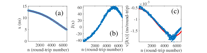
Figure 4: (a) The blue circles represent the localized pulse position within the cavity at each round-trip during the trajectory represented in Fig. 3c). From these data points a continuous trajectory is interpolated and represented in red. (b) The values of the current experienced by the localized pulse at each point of its trajectory. (c) Drifting speed calculated in two different manners. The blue dots corresponds to the instantaneous drifting speed calculated as $v_{J}+v_{\Delta}=0$, and using the values of the bias current experienced by the LS in panel (b) and where the function $v{}_{J}$ has been obtained by fitting the curve $v{}_{J}(J-J_{ref})$ shown in Fig. 2 by circles. The red curves correspond to the derivative of the interpolated trajectory in (a).

III.1 Motion induced by a pumping current landscape

In order to analyze the statics and dynamics of a single localized pulse in a parameter landscape, we modulate the VCSEL pumping current within the multi-stable current region where LSs exist. We define the detuning between the modulation frequency $\nu_{mod}$, and the cavity resonance frequency $\nu_{cav}=1/T$, as $\Delta=\nu_{mod}$-$\nu_{cav}$. The value of $T$ is estimated by using the same procedure described above for a single localized pulse at the steady current value $J=J_{ref}$ around which the modulation is applied.

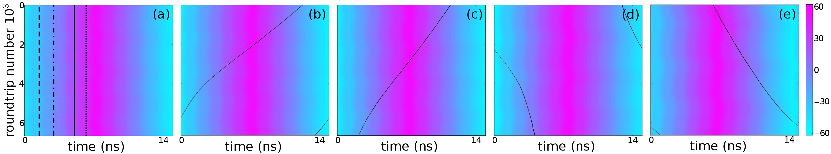
Figure 5: Spatio-temporal diagram of pulse position evolutions when the current is modulated by a triangular waveform of amplitude $A=120\,$mA around $J_{ref}=253\,$mA and at a frequency closed to $\nu_{cav}=66608500\,$Hz. The current values are represented in color scales. a) Four different situations are shown corresponding to stable equilibrium positions for different detuning values: $\Delta=-4\,$kHz (dashed line), $\Delta=-0.5\,$kHz (dot-dashed line), $\Delta=1\,$kHz (continuous line) and $\Delta=1.5\,$kHz (dotted line). Drifting regimes with b)$\Delta=-10.5\,$kHz, c)$\Delta=-6\,$kHz, d) $\Delta=2.5\,$kHz, and e) $\Delta=+6.5\,$kHz.

III.1.1 Sinusoidal modulation

Different modulation signals have been applied, and we start by describing the results obtained with the sinusoidal one, which can be coupled into the laser without being distorted up to the 500 MHz cut-off frequency of our laser module. The modulation amplitude is $A=120\,$mA around $J_{ref}=226\,$mA. In Fig. 3a) we show the evolution of a single pulse for small values of $\Delta$ (-4.75 kHz <$\Delta$< 2.5 kHz) using space-time diagrams. In order to simplify the interpretation of the LS evolution, we have built these diagrams in the reference frame of the modulation signal. Accordingly, the current modulation pattern is always stationary in the space-time diagrams while the LS position may evolve with the number of round-trips. The current modulation is represented in Fig. 3a) using a color scale and it is superimposed to the LS trajectory in order to make evident how the localized pulse behaves onto this current landscape. Figure 3a) shows that, when $\Delta$ is within the range specified above, the pulse position is stationary with respect to the modulation signal and that the stationary position is a function of $\Delta$.

When $\Delta=0$ the localized peak exhibits a fixed position with respect to the modulation signal. This position is located on the positive slope at the point where the modulation signal is equal to zero. It is important to note that, in this stable position for the LS, the derivative of the modulation signal is different from zero. This result points out the difference of our LSs with respect those described by the Lugiato-Lefever equation, which are expected to have a zero speed only where the parameter derivative (or its gradient for spatial systems) is equal to zero JEC-NAC-15 .

If $\Delta\neq 0$, in the reference frame of the modulation signal, the LS experiences a time slip $\delta t$ at every round trip given by the difference between the modulation period and the cavity round-trip. In the space-time representation, this time shift at every round-trip can be interpreted as a detuning-induced drifting speed $v{}_{\Delta}$ given by $v_{\Delta}$=$\frac{\Delta}{\nu_{mod}\nu_{cav}}$ in the limit of $\Delta\ll\nu_{cav}$. Figure 3a), shows that, if $\mid\Delta\mid$ is small enough (-4.75 kHz <$\Delta$< 2.5 kHz), the LS remains in a stationary position with respect to the modulation signal. This equilibrium position gets closer to the modulation peak (bottom) for increasing positive (negative) value of $\Delta$. Moreover, all the stable equilibrium positions found varying $\Delta$ are located on the positive slope of the modulation signal.

These stationary positions for the LSs in presence of a finite detuning indicate that $v_{\Delta}$ must be compensated by an opposite drifting speed $v_{J}$ induced by the current variation around $J_{ref}$, such that $v_{J}+v_{\Delta}=0$. Accordingly, from the stationary positions expressed in terms of the values of the current, it is possible to infer the value of $v_{J}$ as a function of $\left(J-J_{ref}\right)$. These values are represented in Fig. 2 using circles. The curve $v_{J}(J-J_{ref})$, obtained by sinusoidally modulating the bias current, is rather close to the same curve obtained by changing the stationary value of J (crosses connected by red line). When considering that thermal effects induced by current variation become less and less relevant when the current is modulated at high rates, the proximity of the two curves is a further confirmation that thermal effects do not play a relevant role in determining the drifting speed of LS.

Finally, the fact that $\frac{dv{}_{J}}{dJ}<0$, explains also why the equilibrium points, i.e. those points satisfying the condition $v{}_{J}+v{}_{\Delta}=0$, are stable only when located on the positive slope of the modulation while they are unstable when located on the the negative slope. In the former case, any perturbation of the LS position around the fixed points implies a change of the current value experienced by the localized pulse which generates a restoring force, thus bringing back the pulse towards the fixed point. In the latter case, any perturbation implies a change of the current value experienced by the localized pulse which generates a repelling force, thus pushing the pulse farther away from the equilibrium point.

For values of $\Delta$ outside the above specified interval, $v{}_{\Delta}$ cannot be balanced by $v{}_{J}$ at any current values spanned by the modulation and the LS unlocks and starts to drift in the space-time diagram, as shown in Fig. 3b-d). The relative speed is positive (negative) for positive (negative) value of $\Delta$ and it depends on the localized pulse position within the cavity. In the limit where $\Delta$ is very large, $v{}_{J}$ is small compared with $v{}_{\Delta}$ and the drifting speed is almost constant. For values of $\Delta$ around $10\,$kHz, $v{}_{J}$ is comparable to $v{}_{\Delta}$ and the LS accelerate and decelerate as a function of its position inside the cavity, as shown in Fig. 3b-e). By extracting from Fig. 3c) the time law of the localized pulse (shown in Fig. 4a), we calculate the corresponding instantaneous velocity in the space-time diagram (in ps per round-trip) which is represented in Fig. 4c), red curve. From Fig. 3c) it is also possible to extract the values of the current $(J-J_{ref})$ experienced by the localized pulse during its trajectory (Fig. 4b). The curve in Fig. 2 obtained for sinusoidal modulations (circles) can be polynomially fitted and used, together with Fig. 4b), to calculate the value of $v{}_{J}$ at each round-trip. Finally, by adding $v{}_{J}$ and $v{}_{\Delta}$, calculated from the value of $\Delta$, one obtains the blue curve in Fig. 4c), which gives the instantaneous values of LS drifting speed. Within the experimental uncertainty, the two curves in Fig. 4c) coincide, thus evidencing that the instantaneous velocity of the localized pulse depends exclusively on the value of the modulation signal instead of its time derivative.

III.1.2 Triangular modulation

A triangular waveform has been also used for modulating the pumping current. This waveform is interesting because its time derivative features a constant positive value on the ascending triangle slope and the same, but negative, value on the descending triangle slope. Time derivative is zero only at the top and the bottom of the modulation. Accordingly, if the drifting speed was depending on the modulation signal time derivative, the equilibrium position should be located, for $\Delta=0$, on the modulation extrema and the drifting speed should be constant on the slopes of the modulation. Figure 5a) shows the stable equilibrium positions for four different values of the detuning. The stationary positions are located on the positive slope of the signal and they depend on $\Delta$. This is a further confirmation of the negligible dependence of $v{}_{J}$ on the modulation signal derivative, which is a constant on the entire signal positive slope. Similarly to the case of the sinusoidal modulation, the stationary positions of the LS with respect to the modulation signal can be used to infer the value of $v{}_{J}$ induced by a current variation around the steady value $J_{cw}$. The curve $v{}_{J}(J-J_{ref})$ is again plotted in Fig. 2 using diamond markers. The situation is very similar to the one obtained by varying the continuous value of the current and the one obtained by modulating sinusoidally the pumping current. When the detuning is exceedingly large with respect the current variation, the term $v{}_{J}$ can never compensate for the term $v_{\triangle}$ and the localized pulse drifts inside the cavity with a speed per round-trip which is a function of the local value of the current, as shown in Fig. 5b-e). The variations of the speed on the signal slopes give a visual indication that $v{}_{J}$ is a function of current values rather than its derivative.

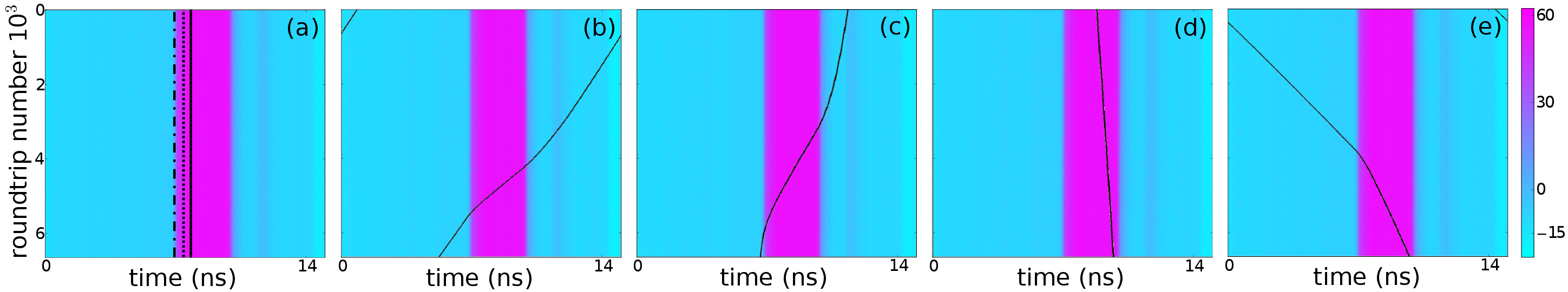
Figure 6: Spatio-temporal diagram of pulse position evolutions (dark trace) when the current is modulated by a rectangular waveform of amplitude $A=76\,$mA around $J_{cw}=221\,$mA and at a frequency close to the resonance $\nu_{cav}=66612500\,$Hz. The current values are represented in color scales. a) Three different situations are shown corresponding to stable equilibrium positions for different detuning values: $\Delta=-1.3\,$kHz (dash-dotted line), $\Delta=1\,$kHz (dotted line) and $\Delta=2.5\,$kHz (continuous line). Out of the locking range, drifting trajectories are depicted for detuning values of b) $\Delta=-7.5\,$kHz, c) $\Delta=-1.9\,$kHz, d) $\Delta=3.8\,$kHz and e)$\Delta=7\,$kHz.

III.1.3 Rectangular modulation

The experimental evidences reported so far indicate that a rectangular current modulation, which introduces a bi-valued current landscape, should enable robust temporal tweezing of localized pulses. Because the current is widely spanned in the vicinity of the rectangle waveform edges, the rising-edge of the signal should be a narrow anchoring region for localized pulses for a wide detuning range. We select a rectangular waveform almost resonant with the cavity free spectral range having a $20\,\%$ duty cycle, which means that current is on the high level for $3\,$ns and on the low level for $12\,$ns. The rise time of the rising edge is 300 ps (10-90 %) and 800 ps (0-100 %). The current profile is not entirely flat after the steep rising edge, and it continues to slightly increase during 450 ps. In Fig. 6 we show the current profile in color scale and the evolution of the localized pulse inside the cavity round-trip after round-trip. In the static case (Fig. 6a), different trajectories of the localized pulse are shown for different values of $\Delta$. The deviation of the current profile from a perfect rectangular shape is not strong enough to be evident on this figure. On the other hand, this deformation explains why the stable fixed positions of the localized pulses for different value of $\Delta$ are not aligned with the rising-edge but they are rather spread on the top of the square modulation. Despite this undesired effect, it is reasonable to claim that the region around the rising-front is an anchoring region for LSs for a wide detuning range (-1.1 kHz <$\Delta$<2.5 kHz). We notice also that, for the same reasons explained for the other waveforms, the falling edge of the pulse only contains unstable equilibrium points. When the detuning is exceeding the locking range, the localized pulse drifts inside the cavity, as shown in Fig. 6b-e). The drifting speed can be roughly considered bi-valued, as it follows the bi-valued current profile. When the value of $\Delta$ is close to the locking range, see Fig. 6c), the speed variation of the localized pulse as it gets close to the edges of the current profile provides a visual demonstration of smooth rising and fall processes of the pumping current.

III.2 Manipulation of Localized Pulses

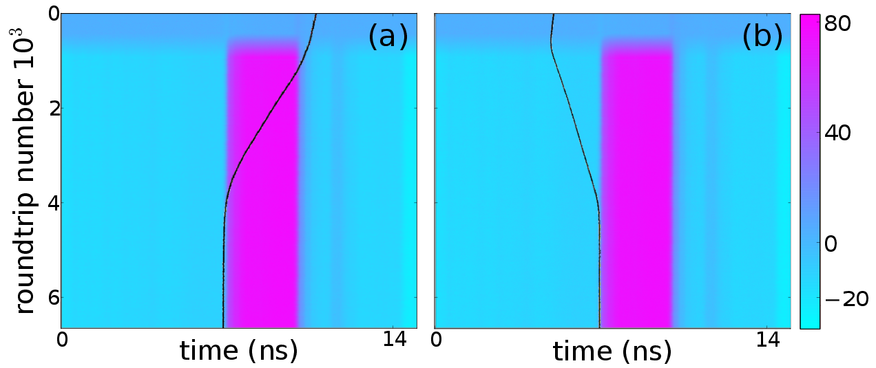
Figure 7: Spatio-temporal diagrams showing the evolution of a localized pulse when an electrical pulse is applied to the pumping current for two different initial positions. The current values are represented in color scales. The Current pulse amplitude is $A=100\,$mA, $J_{cw}=202\,$mA, $\Delta=1.4\,$kHz (left panel) and $\Delta=0\,$kHz (right panel).

The results shown above indicate that current modulation is very effective for manipulating localized pulses. In Fig. 7 we apply an electrical rectangular waveform to the pumping current and we study the dynamics induced on the LS. Wherever the LS is located previously to the application of the current modulation, Fig. 7 shows that it eventually drifts towards the raising edge of the current pulse where it gets anchored. The trajectory for approaching the rising-edge, as well as the final position, depend on the value of $\Delta$. In Fig. 7a), a positive detuning value pushes the LS towards the rising front and, when it reaches the top of the current pulse, this speed is increased by the contribution from the high current level. Eventually the LS sits at the equilibrium point close to the rising edge of the pulse current. In the right panel, the LS is on the left of the current pulse. When the pulse is applied, the current level outside the pulse is slightly decreased with respect to $J_{cw}$ ($\sim 20\,$% of the pulse amplitude) and, as a consequence, the LS experience a drifting speed towards the rising edge of the pulse current. Eventually it sits in the stable equilibrium point on the rising edge.

Localized pulse position manipulation is crucial for applications to information processing. For example, it is important to organize the bit flow inside the cavity according to a precise clock. This can be implemented by introducing a parameter landscape having a period close to a fraction $N$ of the cavity roundtrip ($\nu_{mod}\approxeq N\nu_{cav}$) JEC-NAC-15 . This landscape plays the role of a potential network capable of trapping $N$ localized pulses at fixed time intervals inside the cavity. Despite the modulation bandwidth limitation described in our current set-up, we can still provide a proof-of-principle of this operation by modulating sinusoidally the pumping current at $N=5$, i.e. at $\nu_{mod}\approxeq 5\nu_{cav}$, which allows pinning the position of five localized pulses, as shown in Fig. 8.

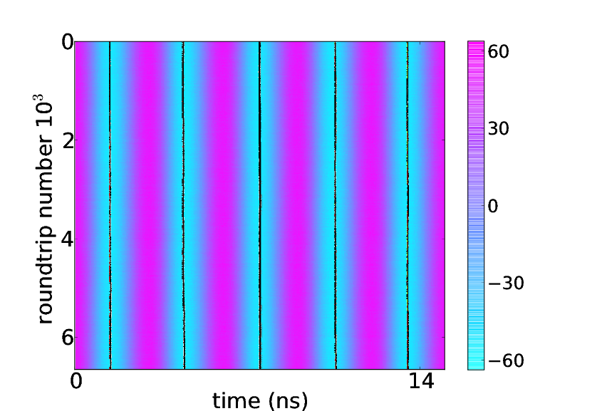
Figure 8: Spatio-temporal diagrams showing five pulses positions evolution (dark trace) in presence of a sinusoidal current modulation at $\nu_{mod}=5\nu_{cav}-4.750\,$kHz, having an amplitude of 120 mA and $J_{cw}=275\,$mA. The current values are represented in color scales.

IV Theory

The existence and dynamics properties of temporal localized structures in passive mode-locked VCSELs have been theoretically described MJB-PRL-14 ; MJB-JSTQE-15 ; MJC-JSTQE-16 using the following delay differential equation (DDE) model VT-PRA-05 :

$$\frac{1}{\gamma}\frac{dA}{dt}+A = \sqrt{\kappa}R\left(t-\tau\right)A\left(t-\tau\right),$$ (1)

$$\frac{dG}{dt} = \Gamma\left(G_{0}-G\right)-e^{-Q}\left(e^{G}-1\right)\left|A\right|^{2},$$ (2)

$$\frac{dQ}{dt} = Q_{0}-Q-s\left(1-e^{-Q}\right)\left|A\right|^{2},$$ (3)

with $R\left(t\right)=\exp\left[\left(1-i\alpha\right)G\left(t\right)/2-\left(1-i\beta\right)Q\left(t\right)/2\right]$, $G_{0}$ the pumping rate, $\Gamma=\tau_{g}^{-1}$ the gain recovery rate, $Q_{0}$ the value of the unsaturated losses which determines the modulation depth of the SA and $s$ the ratio of the saturation energy of the gain and of the SA sections. We define $\kappa$ as the amplitude transmission of the output mirror. In Eqs. (1-3) time has been normalized to the SA recovery time. The frequency filter (that mimics the gain curve) has a bandwidth of $\gamma$ and the cold cavity round-trip is given by the inverse of the time delay $\tau$. The alpha factor of the gain and of the absorber sections are $\alpha$ and $\beta$, respectively. The main usefulness of Eqs. (1-3) is to provide an uniformly accurate description of the whole set of system solutions (including single- and multi- longitudinal modes ones), among which the pulsating mode-locked solutions are only a subset. Accordingly, this model allows to unfold the bifurcation diagram using DDEBIFTOOL DDEBT , thus depicting how the various solution branches are linked one with the others and how temporal LSs appear MJB-PRL-14 .

Elaborating on these results and taking advantage of the long cavities limit at which we operate this system experimentally, we can reduce the dimensionality of the model. Such approach was successfully used in JCM-PRL-16 and also for the theoretical study of light bullets J-PRL-16 . Light bullets, or spatio-temporal localized structures, have strong link with the current work as they share the same mechanism for temporal localization. We will show that this approach allows finding the effective equation of motion for the LS quite directly. The general theory for the effective equation of motion of LS in DDEs will be presented elsewhere.

We start by putting the delayed terms in the left hand side of Eq. 1 and define a smallness parameter as the inverse of the filter bandwidth setting $\varepsilon=1/\gamma$ to find

$$\varepsilon\frac{dA}{dt}\left(t+\tau\right) + A\left(t+\tau\right)=\sqrt{\kappa}R\left(t\right)A\left(t\right).$$ (4)

Physical intuition dictates that the pulse-width scales as the inverse of the filter bandwidth and is proportional to $\gamma^{-1}=\varepsilon$. In a related way, one can foresee that the period of the pulse train scales as $T_{0}\sim\tau+\gamma^{-1}$, i.e. the period is always larger than the delay due to causality and the finite response time of the filtering element. Consequently, the solution is slightly drifting to the left in a space-time diagram in which horizontally is the local time, playing the role of space $z$, and vertically (downward) the round-trip number, playing the role of a slow time $s$. As such, we assume that the solution is composed of two time scales and write

$$\frac{d}{dt} \rightarrow \frac{\partial}{\partial x}+\varepsilon^{2}\frac{\partial}{\partial s}$$ (5)

and, following GP-PRL-96 , we express the delayed term as

$$A\left(t+\tau\right) = A\left(x+\varepsilon\upsilon,s+\varepsilon^{2}\tau\right)$$ (6)

This implies that the solution is allowed to evolve on the slow time scale but also to drift on the fast one with an unknown drift velocity $\upsilon$. We find that

$$A\left(t+\tau\right) = A+\varepsilon\upsilon\frac{\partial A}{\partial x}+\frac{\left(\varepsilon\upsilon\right)^{2}}{2}\frac{\partial^{2}A}{\partial x^{2}}$$ (7)

$$+ \varepsilon^{2}\tau\frac{\partial A}{\partial s}+\mathcal{O}\left(\varepsilon^{3}\right)$$

$$\varepsilon\frac{dA}{dt}\left(t+\tau\right) = \varepsilon\left[\frac{\partial}{\partial x}+\varepsilon^{2}\frac{\partial}{\partial s}\right]A\left(t+\tau\right)$$ (8)

$$= \varepsilon\frac{\partial A}{\partial x}+\varepsilon^{2}\upsilon\frac{\partial^{2}A}{\partial x^{2}}+\mathcal{O}\left(\varepsilon^{3}\right)$$ (9)

yielding up to $\mathcal{O}\left(\varepsilon^{3}\right)$

$$\left(\varepsilon\frac{d}{dt}+1\right)A\left(t+\tau\right) = A+\varepsilon\left(\upsilon+1\right)\frac{\partial A}{\partial x}$$

$$+ \left[\frac{\left(\varepsilon\upsilon\right)^{2}}{2}+\varepsilon^{2}\upsilon\right]\frac{\partial^{2}A}{\partial x^{2}}+\varepsilon^{2}\tau\frac{\partial A}{\partial s}$$

Since we introduced a drift term in order to obtain steady solutions, we consistently cancel the first order spatial derivative and set $\upsilon=-1$. In other words, the solution at the next round-trip, is $A\left(z-\gamma^{-1}\right)$ that is to say, it is shifted to the left which precisely corresponds to a period of $T_{0}=\tau+\gamma^{-1}$.

Interestingly, we find that the pulse filtering is represented by a diffusion term of magnitude $\upsilon^{2}/2$ highlighting that filtering and period deviation with respect to $\tau$ are intimately related and eventually boil down to causality and finite response time of the filtering element. In this approach where we factored out the drift of the filtering element, the residual drift terms will only be due to the nonlinear interactions with the gain and the absorber.

We finally find, redefining the time by the value of the round-trip as $\sigma=\varepsilon^{-2}s/\tau$ and setting $I=\left|A\right|^{2}$

$$\frac{\partial A}{\partial\sigma}-\frac{1}{2\gamma^{2}}\frac{\partial^{2}A}{\partial z^{2}} = \left\{\sqrt{\kappa}e^{\frac{1-i\alpha}{2}G-\frac{1-i\beta}{2}Q}-1\right\}A,$$ (11)

$$\frac{\partial G}{\partial z}+\frac{1}{\tau}\frac{\partial G}{\partial\sigma} = \Gamma\left(G_{0}-G\right)-e^{-Q}\left(e^{G}-1\right)I,$$ (12)

$$\frac{\partial Q}{\partial z}+\frac{1}{\tau}\frac{\partial Q}{\partial\sigma} = Q_{0}-Q-s\left(1-e^{-Q}\right)I,$$ (13)

The equations (11-13) are subject to the following periodic boundary condition

$$A\left(z+T_{0},t\right) = A\left(z,t\right)$$ (14)

The Eqs. (11-13) can be understood as a generalization of the Haus master equation to large gain and absorption which is in itself interesting. Indeed, one of the main advantage of the model of VT-PRA-05 is the consideration of large gain and absorption, a feature that is still preserved by the exponential terms in the above PDE.

In order to reduce further the complexity of the model presented in Eqs. (11-13), we take the limit of small gain and absorption setting $G\sim Q\sim 0.1$ which is still a sensible approximation even in the case of semiconductor lasers, so that we can expand the exponential to first order and we also take the long delay limit in which $\tau^{-1}\partial_{\sigma}\left(G,Q\right)\ll 1$ allowing us to keep only the spatial derivative contribution in the gain and the absorber to find with $d=\left(2\gamma^{2}\right)^{-1}$

$$\negthickspace\negthickspace\negthickspace\negthickspace\negthickspace\negthickspace\frac{\partial A}{\partial t} \negthickspace=\negthickspace \left[\sqrt{\kappa}\left(1+\frac{1-i\alpha}{2}G-\frac{1-i\beta}{2}Q\right)-1+d\frac{\partial^{2}}{\partial z^{2}}\right]\negthickspace A,$$ (15)

$$\negthickspace\negthickspace\negthickspace\negthickspace\negthickspace\negthickspace\frac{\partial G}{\partial z} \negthickspace=\negthickspace \Gamma G_{0}-G\left(\Gamma+\left|A\right|^{2}\right),\frac{\partial Q}{\partial z}\negthickspace=\negthickspace Q_{0}-Q\left(1+s\left|A\right|^{2}\right),$$ (16)

which was the model directly used in JCM-PRL-16 .

IV.1 Single LS solution branch

We search for solutions of Eqs. (15-16) with a possible drift $\upsilon$ and a carrier frequency $\omega$ as

$$A\left(z,\sigma\right) = A_{0}\left(z-\upsilon\sigma\right)e^{-i\omega\sigma}$$ (17)

which adds in the right-hand side of Eq. (15) a term $\left(\upsilon\partial_{z}+i\omega_{0}\right)A_{0}$. Here, the influence of the drift $\upsilon$ results from the nonlinear interaction with the active media that have non-instantaneous responses. Although the full bifurcation diagram of Eq. (15) could be obtained with software as pde2path pde2path , as we restrict our analysis to the stable solution branch, a bifurcation diagram can be obtained by direct numerical integration. We solved the Eqs. (15-16) via a Fourier based semi-implicit split-step method as in MJB-JSTQE-15 . A typical profile can be observed in Fig. 9. Here, the value of the solution parameters $\left(\upsilon,\omega\right)$ were determined self-consistently by imposing the stationarity of $A_{0}$ as well as a proper phase condition. It is interesting to notice how this method reduces the complexity of the problem as compared with the original formulation of the problem as a DDE system. Here, one does not need to consider a full domain of size $T_{0}\sim\tau$ corresponding to the full extent of the time period imposed by the large time delay. In our case, the effective numerical domain is kept only a few time larger than the optical pulse, which remains however much smaller than the actual extent of the LS, that is governed by the recovery of the slowest variable $G$. Since the field decays to zero before and after the emission of the LS, it is not affected by the “wrong” periodic boundary conditions imposed by the spectral algorithm we used.

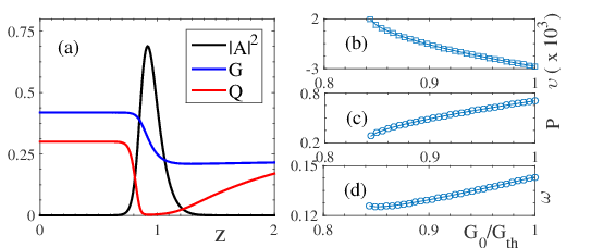
Figure 9: (a) Localized pulse profile in terms of the field intensity, the carrier and the absorption with $G=0.99G_{th}$. Panels (b), (c) and (d) depict the drift velocity $\upsilon$, the pulse integrated energy $P$ and the residual frequency $\omega$ along the stable solution branch. Parameters are $\left(\gamma,\kappa,\alpha,\beta,\Gamma,Q_{0},s\right)=\left(40,0.8,1,0.5,0.04,0.3,30\right)$.

A typical LS profile as well as its bifurcation diagram are depicted in Fig. 9. A typical asymmetrical profile can be observed in Fig. 9(a) while the bifurcation diagrams for $\upsilon$, $P$ and $\omega$ are depicted in Fig. 9(b-d). Importantly, the drift velocity (or equivalently the deviation of the period with respect to the period $T_{0}$) is a decreasing function of the bias current, as found experimentally. As we will show later, this implies that the interaction between distant LSs is purely repulsive. One notices in Fig. 9c) that the solution branch for the energy of the pulse as defined as $P=\int_{-\infty}^{\infty}|A\left(z,t\right)|^{2}dz$ shows the typical square-root behavior consistent with the fact that the single LS solution arises as a saddle-node bifurcation of limit cycle, as demonstrated in the bifurcation diagram of Eqs. (1,3) discussed in MJB-PRL-14 .

The fact that the solution branch exhibits a predominant drift in a particular direction can be ascribed to the lack of spatial reversibility $z\rightarrow-z$ in our system that is apparent in the carrier equations Eqs. (16) having only first order derivative in space. It is worthwhile noting that an adiabatic elimination of the carrier over the fast temporal variable ($z$), leading to $G=G_{0}/\left(1+|A\left(z,t\right)|^{2}/\Gamma\right)$, and, similarly for the absorption, would cancel such a drifting solution and reduce Eq. (15) to a generalized Ginzburg-Landau Equation as in RK-OS-88 . While the latter adiabatic elimination of $Q$ could represent some realistic experimental conditions, the former elimination of $G$ is incorrect in a semiconductor medium since the recovery time of the gain $\tau_{g}$ is much longer than the pulsewidth $\tau_{p}\sim\gamma^{-1}$.

IV.2 Derivation of the EEM

We now outline our approach for deriving the EEM. Well separated LSs interact via the overlap of their tails. In particular, the interaction between two consecutive LSs is mediated by the left (resp. right) tail of the rightmost (resp. leftmost) LS. As the LSs considered in this manuscript are multi-components and multiscales objects, their interactions are somehow peculiar. The inspection of Fig. 9a) shows that the rising front is very short; it is governed by the timescale related to the optical pulse, which is of the order of a few picoseconds and controlled by the bandwidth of the filtering element $\gamma$. The black line in Fig. 9a) corresponds to an intensity rising as $I\sim\exp\left(\gamma t\right)$. Oppositely, the right decaying tail is dominated by the gain recovery that scales as $G\sim\exp\left(-\Gamma t\right)$, which can be appreciated by the almost horizontal blue line in Fig. 9(a) following the gain depletion. As the difference between $\gamma$ and $\Gamma$ amounts to several order of magnitudes ($\gamma/\Gamma\sim 10^{3}$), the leftmost LS will influence the rightmost one via its tail induced by the gain recovery, while the reciprocal interaction will be completely negligible. In this respect, and as compared to the standard cases in the literature regarding the interaction between cavity solitons MBH-PRE-00 , our situation is counter-intuitive as the interactions violate completely the action-reaction principle. In our case, the “reaction” is completely negligible.

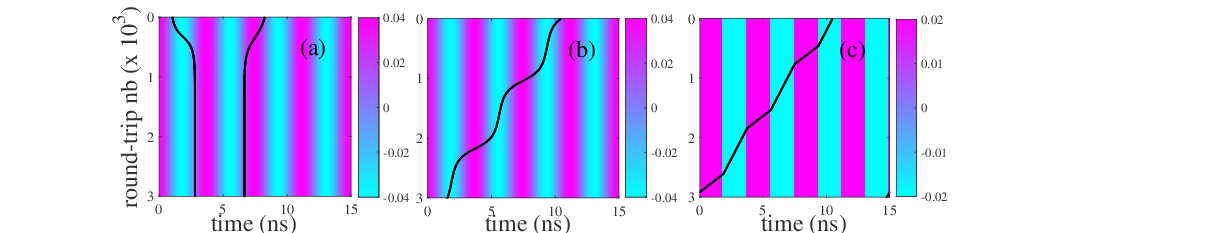
Figure 10: (a) Resonant harmonic potential: The LS goes to the rising front and escape of the falling front that corresponds to the stable and the unstable fixed points, respectively. (b) Strongly detuned harmonic potential; The LS motion corresponds to unlocked trajectories. Here, the LS slows down around and accelerate periodically. (c) Strongly detuned motion beyond the locking range but in a square potential: Note how the speed is simply bi-valued for the square modulation yielding a broken line trajectory. The frequency of the external modulation corresponds to the fourth harmonic $\omega_{ext}=4/T_{0}$ with $T_{0}=15\,$ns. The amplitude of the harmonic (a-b) and square (b) modulation is $A=0.04$ and $A=0.02$, respectively. The detuning between the natural LS motion and the external periodic potential are represented by different values of $\upsilon_{\Delta}$ and reads (a) $\upsilon_{\Delta}=-2.35\times 10^{-3}$ (no detuning), (b) $\upsilon_{\Delta}=-1\times 10^{-3}$ and (c) $\upsilon_{\Delta}=-1.3\times 10^{-3}$. The current values are represented in color scales.

We can use the fact that the interactions will be dominated by the slowest variable $G$ to build the EEM simply, without the need to solve the adjoint problem associated with Eqs. (15,16) as detailed for instance in VFK-JOB-99 ; MBH-PRE-00 . Close to a saddle-node bifurcation, an excellent approximation is found for the drift velocity and the pulse energy with a square root ansatz and we denote

$$\upsilon =f\left(G_{0}\right)= \upsilon_{0}+\Delta\upsilon\sqrt{G_{0}-G_{sn}}$$ (18)

$$P =h\left(G_{0}\right)= P_{0}+\Delta P\sqrt{G_{0}-G_{sn}}$$ (19)

with the coefficients $\left(\upsilon_{0},\Delta\upsilon,P_{0},\Delta P\right)=\left(2\times 10^{-3},-10^{-2},0.28,0.7\right)$ and $G_{sn}=0.845G_{th}$ given by the best fit of the bifurcation diagram of a single LS in Fig. 9. From these results we can now obtain the EEMs for an ensemble of interacting LS in a periodic potential directly. We allow for the general case of a periodic potential whose period is slightly different than the natural resonance of the system. By going in the reference frame of the external periodic potential, the equation for the relative drift velocity Eq. (18) simply becomes

$$\tilde{\upsilon}+\upsilon_{m} = f\left(G_{0}\right)$$ (20)

with $\upsilon_{m}$ the velocity of the drifting potential and $\tilde{\upsilon}$ the residual speed due to the interactions of the pulse with the gain. In this reference frame, the external potential depends only on the fast time $\left(z\right)$ and not anymore on the slow time $\left(\sigma\right)$. Our main hypothesis consists in saying that, with a spatially dependent gain, the solution are now depending on the local value of the gain at the leading edge of the pulse $G^{\left(i\right)}$, i.e. we replace in Eqs. (18,19) $G_{0}\rightarrow G^{\left(i\right)}$. By allowing each LS to imprint a gain depletion and considering the partial gain recovery in-between LS, we will automatically obtain the EEMs. We recall that the gain at the falling edge of the pulse is simply

$$G^{\left(f\right)} = G^{\left(i\right)}\exp\left(-P\right).$$ (21)

In between LS, during the so-called slow stages where the gain recovers, the evolution of $G$ is governed by

$$\frac{\partial G}{\partial z} = \Gamma\left[G_{0}\left(z\right)-G\right],$$ (22)

Provided that the variations of the bias current $G_{0}\left(z\right)$ are slower than the typical relaxation time $\tau_{g}$, i.e. $\Gamma\dot{G}_{0}\ll G_{0}$, the solution of the carrier equation Eq. (16) reads

$$G\left(z_{2}\right) = G\left(z_{1}\right)e^{-\Gamma\Delta z}+G_{0}\left(z_{2}\right)\left(1-e^{-\Gamma\Delta z}\right)$$ (23)

where $\Delta z=z_{2}-z_{1}$ corresponds to the “distance” between two LSs and $G\left(z_{1}\right)$ is the initial condition. Hence, by denoting as $z_{n}$ the position of the $n$-th LS whose residual velocity is $\tilde{\upsilon}_{n}=dz_{n}/d\sigma$, we find that

$$\frac{dz_{n}}{d\sigma} = f\left(G_{n}^{\left(i\right)}\right)-\upsilon_{m}\;,\;P_{n}=h\left(G_{n}^{\left(i\right)}\right)$$ (24)

$$G_{n}^{\left(i\right)} = G_{n-1}^{\left(i\right)}\exp\left[-P_{n-1}-\Gamma\left(z_{n}-z_{n-1}\right)\right]$$ (25)

$$+ G_{0}\left(z\right)\left(1-\exp\left[-\Gamma\left(z_{n}-z_{n-1}\right)\right]\right)$$

where we replaced the initial condition $G_{n-1}^{\left(f\right)}$ at the falling edge of the $\left(n-1\right)$-th LS located in $z_{n-1}$ by $G_{n-1}^{\left(f\right)}=G_{n-1}^{\left(i\right)}\exp\left(-P_{n-1}\right)$. For $N-$LS with $n\in\left[1,\dots,N\right]$, the periodic boundary conditions linking the gain depletion of the rightmost LS to the dynamics of the leftmost one reads

$$z_{0} = z_{N}-T_{0}.$$ (26)

Some general considerations regarding the EEMs can already be drawn. The unidirectional interaction between LS is visible in Eq. (25) where $G_{n}^{\left(i\right)}$ only depends on $z_{n}$, $z_{n-1}$ but not $z_{n+1}$. Also, a great advantage of the EEMs is that the problem does not become more stiff when the value of the delay increases; While the cost of a direct integration of Eqs. (1-3) scales linearly with the value of the time delay, the one of the EEMs remains constant. Secondly, the dynamics of a large ensemble of interacting LS, possibly in a periodic potential and in the presence of noise, can be studied via a molecular dynamics approach where each LS is represented by a point like particle in interactions with its nearest neighbors. Finally, long simulations are desirable if one wishes to compare with experimental results, in which the acquisition time amounts to $10^{4}\sim 10^{5}$ round-trips, which can be done with the EEMs easily. If not otherwise stated, the parameters of the EEMs are $\left(\upsilon_{0},\Delta\upsilon,P_{0},\Delta P\right)=\left(0,-0.01,0.28,0.7\right)$ while $G_{sn}=0.845G_{th}$ and the current value is $G_{0}=0.9G_{th}$. These parameters were obtained making a best fit of Fig. 9b-d).

IV.3 Motion in a periodic potential

In the case where the potential period is resonant with that of a single LS, it can be demonstrated from a linear stability analysis that the stable fixed point corresponds to the zero of the rising front of the modulation. On the contrary, the falling edge is a saddle point, due to the fact that $\Delta\upsilon<0$ in Eq. (18). Figure 10a) shows how two initial conditions on each side of a saddle points over the falling edges, give rise to two different trajectories. In presence of a detuning between the modulation and the natural period of the LS motion, the stable and the unstable equilibrium positions grow closer up to their disappearance in a saddle-node bifurcation, very much similar to the Adler bifurcation to unlocked states. A typical unlocked trajectory is depicted in Fig. 10b). Finally, we represent in Fig. 10c) the unlocked motion in a bi-valuated square potential.

IV.4 Interactions between LSs

We start by considering the case of the self-interaction of a single LS. The gain depletion generated in the wake of a LS has to be connected to itself after a single round-trip, we therefore set $z_{n}-z_{n-1}=T_{0}$ and $G_{n}=G_{1}\,\forall n$ which allows us to find solving Eq. (25) the value of the leading edge gain

$$G_{1} = r_{1}G_{0},$$ (27)

with the following expression for $r_{1}$

$$r_{1} = \frac{1-e^{-\Gamma T_{0}}}{1-e^{-\Gamma T_{0}-P}}.$$ (28)

The factor $r_{1}<1$ represents the gain reduction induced by the presence of a single LS as compared to the nominal value $G_{0}$ found only when the cavity is empty. It represents the self-crowding induced by the LS due to its own gain saturation, if the cavity is not sufficiently long. This effect of course disappears in the long delay limit $\Gamma T_{0}\gg 1$ where $r_{1}\rightarrow 1$.

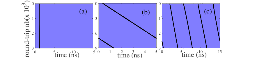
Figure 11: Effect of self and mutual interactions between LS. Notice how the drift velocity is affected by the effect of self interactions as the only difference between panels (a) and (b) is the length of the cavity. Mutual interactions in a regular crystal structure presented in (c) also influence the drifting speed with respect to (a).

A similar result can be found for $N$ equidistant LSs for which we simply replace $T_{0}\rightarrow T_{0}/N$ in Eq. (28) which allows finding $r_{N}$. In particular, one deduces that the $N-$LSs solution will have a different gain than a single LS solution. This effect can be linked to the global coupling found for spatial LSs which was shown to induce a slanting in their bifurcation diagram, the so-called homoclinic snaking FCS-PRL-07 . Besides defining a more limited domain of existence, which was studied in MJB-PRL-14 , see Fig. 2d, it will also induce a change in their drift velocity. As the speed $\upsilon$ is a function of $G$, this effect can be appreciated in Fig. 11a,c), where one can see that the solutions with $N=1$ and $N=4$ have different drifts. In addition, the difference of gain and therefore of drifting speed as a function of the cavity length is depicted in Fig. 11b) for the case with $N=1$.

Finally, we conclude our analysis in Fig. 12a), where the asymmetrical repulsive interaction between nearby LSs is made apparent. Here the first LS affects the second one but not the other way around. The source of the asymmetry is contained in Eq. (12) where each LS with position $z_{n}$ is only coupled to its previous neighbor $z_{n-1}$. This theoretical prediction can be compared with experimentally obtained trajectories of multiple localized pulses (Fig. 1) where the asymmetric character of the interaction is evident. However, these interactions are weak and occurs on very long time scales. As soon as a external modulation is applied as in Fig. 12b), the LSs dynamics becomes dominated by the interaction potential.

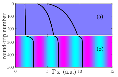
Figure 12: (a) Asymmetrical interactions between nearby LSs. As soon as an external modulation is applied (b) the LSs fall at the bottom of the induced potential. The amplitude of the sinusoidal modulation is $A=0.04$ and the current values are represented in color scales.

V Conclusions

In this manuscript we have shown that temporal LSs in a passively mode-locked semiconductor laser system can be addressed by using current electrical pulses. Despite the limited electrical bandwidth of our laser module, which prevent us from addressing more than one localized pulse per round-trip, it is important to underline that this method can lead to a robust and a convenient LS addressing scheme at GHz rates. These localized pulses exist for a wide range (typically more than 100 mA) of the VCSEL pumping current $J$ and, similarly to spatial LS, they can be used as bits for information processing. A bit stream can be written inside the cavity at an addressing rate fixed by the temporal width of the LS. More precisely, even if in terms of the output intensity the LS obtained exhibit a temporal width of approximately 10 ps, their width is ultimately fixed by the underlying gain recovery process which has an effective exponential time constant of a few nanoseconds. As the plasticity of the LSs spatial configuration renders their individual control possible, the laser bias current has been used for introducing a parameter landscape and controlling the position of the localized pulses inside the cavity. In this respect, we have disclosed a new paradigm for LS manipulation where the induced drifting speed does not depend upon the gradient of the parameter landscape but, instead, on its local value, which we traced back to the strong asymmetry of the LS temporal profile whose rise and fall time are typically in the picosecond and the nanosecond range, respectively. We have provided a proof of principle for localized pulse position reconfiguration using electrical square modulation and we have shown that a weak amplitude current modulation can be used to precisely clock the position of the flow of localized pulses inside the cavity. Our experimental findings where supported by a theoretical analysis based upon a generic delay differential equation model. However as the LS dynamics evolves significantly only over a very large number of round-trips, that are in addition very long as compared to the usual situations, we simplified our DDE model into an equivalent Haus master equation that we were able to solve efficiently by exploiting the long delay limit. This allowed to reduce the numerical domain to a few times the extend of the optical component of the LS, and neglect the long tail of the gain recovery. This tail can be obtained analytically and its asymptotic value used to set the proper boundary conditions. From the evolution of the LS drift velocity as a function of the gain, we were able to write the effective equation of motions for each LS as it they were rigid pseudo-particles governed only by weak nearest neighbor interactions. These analytical results enabled us to confirm the most important experimental findings, namely the presence of strongly asymmetrical interactions and the existence of equilibrium points in the vicinity of the rising front of the external modulation.

- (1) J. Wu, R. Keolian, and I. Rudnick. Observation of a nonpropagating hydrodynamic soliton. Phys. Rev. Lett., 52:1421–1424, Apr 1984.
- (2) E. Moses, J. Fineberg, and V. Steinberg. Multistability and confined traveling-wave patterns in a convecting binary mixture. Phys. Rev. A, 35:2757–2760, Mar 1987.
- (3) F. J. Niedernostheide, M. Arps, R. Dohmen, H. Willebrand, and H. G. Purwins. Spatial and spatio-temporal patterns in pnpn semiconductor devices. physica status solidi (b), 172(1):249–266, 1992.
- (4) P. B. Umbanhowar, F. Melo, and H. L. Swinney. Localized excitations in a vertically vibrated granular layer. Nature, (382):793–796, 1996.
- (5) Yuri A. Astrov and H.G. Purwins. Plasma spots in a gas discharge system: birth, scattering and formation of molecules. Physics Letters A, 283(5-6):349 – 354, 2001.
- (6) N. N. Rosanov and G. V. Khodova. Autosolitons in nonlinear interferometers. Opt. Spectrosc., 65:449–450, 1988.
- (7) M. Tlidi, P. Mandel, and R. Lefever. Localized structures and localized patterns in optical bistability. Phys. Rev. Lett., 73:640–643, Aug 1994.
- (8) W. J. Firth and A. J. Scroggie. Optical bullet holes: Robust controllable localized states of a nonlinear cavity. Phys. Rev. Lett., 76:1623–1626, Mar 1996.
- (9) L.A. Lugiato. Introduction to the feature section on cavity solitons: An overview. Quantum Electronics, IEEE Journal of, 39(2):193–196, 2003.
- (10) O. Thual and S. Fauve. Localized structures generated by subcritical instabilities. J. Phys. France, 49:1829–1833, 1988.
- (11) S. Fauve and O. Thual. Solitary waves generated by subcritical instabilities in dissipative systems. Phys. Rev. Lett., 64:282–284, Jan 1990.
- (12) S. Barland, J. R. Tredicce, M. Brambilla, L. A. Lugiato, S. Balle, M. Giudici, T. Maggipinto, L. Spinelli, G. Tissoni, T. Knödl, M. Miller, and R. Jäger. Cavity solitons as pixels in semiconductor microcavities. Nature, 419(6908):699–702, Oct 2002.
- (13) P. Genevet, S. Barland, M. Giudici, and J. R. Tredicce. Cavity soliton laser based on mutually coupled semiconductor microresonators. Phys. Rev. Lett., 101:123905, Sep 2008.
- (14) Y. Tanguy, T. Ackemann, W. J. Firth, and R. Jäger. Realization of a semiconductor-based cavity soliton laser. Phys. Rev. Lett., 100:013907, Jan 2008.
- (15) T. Elsass, K. Gauthron, G. Beaudoin, I. Sagnes, R. Kuszelewicz, and S. Barbay. Fast manipulation of laser localized structures in a monolithic vertical cavity with saturable absorber. Applied Physics B, 98(2-3):327–331, 2010.
- (16) F. Leo, S. Coen, P. Kockaert, S.P. Gorza, P. Emplit, and M. Haelterman. Temporal cavity solitons in one-dimensional kerr media as bits in an all-optical buffer. Nat Photon, 4(7):471–476, Jul 2010.
- (17) T. Herr, V. Brasch, J. D. Jost, C. Y. Wang, N. M. Kondratiev, M. L. Gorodetsky, and T. J. Kippenberg. Temporal solitons in optical microresonators. Nature Photonics, 8(2):145–152, 2014.
- (18) J. M. McSloy, W. J. Firth, G. K. Harkness, and G.-L. Oppo. Computationally determined existence and stability of transverse structures. ii. multipeaked cavity solitons. Phys. Rev. E, 66:046606, Oct 2002.
- (19) F. Pedaci, P. Genevet, S. Barland, M. Giudici, and J. R. Tredicce. Positioning cavity solitons with a phase mask. Applied Physics Letters, 89(22):221111, 2006.
- (20) F. Pedaci, S. Barland, E. Caboche, P. Genevet, M. Giudici, J. R. Tredicce, T. Ackemann, A. J. Scroggie, W. J. Firth, G.-L. Oppo, G. Tissoni, and R. Jäger. All-optical delay line using semiconductor cavity solitons. Applied Physics Letters, 92(1):011101, 2008.
- (21) Jae K. Jang, Miro Erkintalo, Stephane Coen, and Stuart G. Murdoch. Temporal tweezing of light through the trapping and manipulation of temporal cavity solitons. Nat Commun, 6, Jun 2015. Article.
- (22) Francesco Marino, Giovanni Giacomelli, and Stephane Barland. Front pinning and localized states analogues in long-delayed bistable systems. Phys. Rev. Lett., 112:103901, Mar 2014.
- (23) T. ; Hurtado A. Javaloyes, J. ; Ackemann. Arrest of domain coarsening via anti-periodic regimes in delay systems. Phys. Rev. Lett., 115:223901, Nov 2015.
- (24) M. Marconi, J. Javaloyes, S. Balle, and M. Giudici. How lasing localized structures evolve out of passive mode locking. Phys. Rev. Lett., 112:223901, Jun 2014.
- (25) B. Garbin, J. Javaloyes, G. Tissoni, and S. Barland. Topological solitons as addressable phase bits in a driven laser. Nat. Com., 6, 2015.
- (26) B. Romeira, R. Avó, José M. L. Figueiredo, S. Barland, and J. Javaloyes. Regenerative memory in time-delayed neuromorphic photonic resonators. Scientific Reports, 6:19510 EP –, Jan 2016. Article.
- (27) M. Marconi, J. Javaloyes, S. Balle, and M. Giudici. Vectorial dissipative solitons in vertical-cavity surface-emitting lasers with delays. Nature Photonics, 2015.
- (28) M. Marconi, J. Javaloyes, S. Balle, and M. Giudici. Passive mode-locking and tilted waves in broad-area vertical-cavity surface-emitting lasers. Selected Topics in Quantum Electronics, IEEE Journal of, 21(1):85–93, Jan 2015.
- (29) Roger L. Freeman. Telecommunication System Engineering. John Wiley & Sons, 2015.
- (30) J. Javaloyes, P. Camelin, M. Marconi, and M. Giudici. Dynamics of localized structures in systems with broken parity symmetry. Phys. Rev. Lett., 116:133901, Mar 2016.
- (31) P. Coullet, C. Riera, and C. Tresser. A new approach to data storage using localized structures. Chaos, 14:193–201, Mar 2004.
- (32) P. Coullet, C. Riera, and C. Tresser. Stable static localized structures in one dimension. Phys. Rev. Lett., 84:3069–3072, Apr 2000.
- (33) F. T. Arecchi, G. Giacomelli, A. Lapucci, and R. Meucci. Two-dimensional representation of a delayed dynamical system. Phys. Rev. A, 45:R4225–R4228, Apr 1992.
- (34) G. Giacomelli and A. Politi. Relationship between delayed and spatially extended dynamical systems. Phys. Rev. Lett., 76:2686–2689, Apr 1996.
- (35) M. Marconi, J. Javaloyes, P. Camelin, D. Chaparro, S. Balle, and M. Giudici. Control and generation of localized pulses in passively mode-locked semiconductor lasers. Selected Topics in Quantum Electronics, IEEE Journal of, PP(99):1–1, 2015.
- (36) A. G. Vladimirov and D. Turaev. Model for passive mode locking in semiconductor lasers. Phys. Rev. A, 72:033808, Sep 2005.
- (37) K. Engelborghs, T. Luzyanina, and G. Samaey. Dde-biftool v. 2.00: a matlab package for bifurcation analysis of delay differential equations. Technical report, Department of Computer Science, K.U.Leuven, Belgium., 2001.
- (38) J. Javaloyes. Cavity light bullets in passively mode-locked semiconductor lasers. Phys. Rev. Lett., 116:043901, Jan 2016.
- (39) H. Uecker, D. Wetzel, and J. Rademacher. pde2path - a matlab package for continuation and bifurcation in 2d elliptic systems. Numerical Mathematics: Theory, Methods and Applications, 7:58–106, 2014.
- (40) T. Maggipinto, M. Brambilla, G. K. Harkness, and W. J. Firth. Cavity solitons in semiconductor microresonators: Existence, stability, and dynamical properties. Phys. Rev. E, 62:8726–8739, Dec 2000.
- (41) A. G. Vladimirov, S. V. Fedorov, N. A. Kaliteevskii, G. V. Khodova, and N. N. Rosanov. Numerical investigation of laser localized structures. Journal of Optics B: Quantum and Semiclassical Optics, 1(1):101, 1999.
- (42) W. Firth, L. Columbo, and A. Scroggie. Proposed resolution of theory-experiment discrepancy in homoclinic snaking. Phys. Rev. Lett., 99:104503, Sep 2007.