A Near-Quadratic Lower Bound for the Size of Quantum Circuits of Constant Treewidth

Abstract

We show that any quantum circuit of treewidth $t$, built from $r$-qubit gates, requires at least $\Omega(\frac{n^{2}}{2^{O(r\cdot t)}\cdot\log^{4}n})$ gates to compute the element distinctness function. Our result generalizes a near-quadratic lower bound for quantum formula size obtained by Roychowdhury and Vatan [SIAM J. on Computing, 2001]. The proof of our lower bound follows by an extension of Nečiporuk’s method to the context of quantum circuits of constant treewidth. This extension is made via a combination of techniques from structural graph theory, tensor-network theory, and the connected-component counting method, which is a classic tool in algebraic geometry.

Keywords: Super-Linear Lower Bounds, Quantum Circuits, Algebraic Tensor Networks,
blablablablab Treewidth

1 Introduction

Proving superlinear lower bounds on the size of circuits computing some function in NP remains one of the greatest challenges of computational complexity theory [12, 17, 20]. Currently, the best known lower bound for a function in NP is of the order of $5n-o(1)$ for Boolean circuits with gates from the binary De-Morgan basis [17, 20] and of the order of $(3+1/86)n+o(n)$ for Boolean circuits with arbitrary fan-in-2 gates [12]. Therefore, research in this direction has focused on lower bounds for restricted classes of circuits. In particular, superlinear lower bounds have been proved for Boolean formulas, and for formulas constructed from non-Boolean gates. The strongest known size lower bound for Boolean formulas over the complete binary basis, which is of the order of $\Omega(n^{2}/\log n)$, is due to Nečiporuk [22] and remains unimproved for four decades. If we restrict ourselves to formulas over the De Morgan basis ($\wedge$,$\vee$,$\neg$), then the best known lower bound is of the order of $n^{3-o(1)}$ [15]. Turán and Vatan proved an $\Omega(n^{2}/\log^{2}n)$ size lower bound for arithmetic formulas, and an $\Omega(n^{3/2}/\log n)$ size lower bound for threshold formulas [28]. Yao introduced the notion of quantum formulas (i.e. quantum circuits whose whose underlying graph is a tree) and proved a slightly superlinear lower bound on the size of quantum formulas computing the majority function [31]. Subsequently, Roychowdhury and Vatan proved an $\Omega(n^{2}/\log^{2}n)$ size lower bound for quantum formulas [27].

The treewidth of a graph is a parameter that has played a central role in several branches of algorithmics, combinatorics and structural graph theory [25, 11, 3, 4, 8]. The notion of treewidth has also caught attention from the circuit complexity community due to the fact that the satisfiability of read-once Boolean circuits of constant treewidth can be determined in polynomial time [1, 2, 5, 13, 14, 16, 18]. Recently, near-quadratic lower bounds were shown for Boolean circuits of constant treewidth [9]. In the context of quantum computation, it has been shown that the satisfiability of read-once quantum circuits of constant treewidth can be determined in polynomial time [9]. Additionally, in a pioneering result, Markov and Shi have shown that quantum circuits of constant treewidth can be simulated with multiplicative precision in polynomial time [21].

In this work we prove near-quadratic size lower bounds for quantum circuits of constant treewidth. More precisely, our main result (Theorem 7.3) states that any quantum circuit of treewidth $t$, built from $r$-qubit gates, requires at least $\Omega(\frac{n^{2}}{2^{O(r\cdot t)}\cdot\log^{4}n})$ gates to compute the $n$-bit element distinctness function. In particular, our result imply near-quadratic size lower bounds for several natural restrictions of circuits. For instance, formulas have treewidth at most $1$, TTSP series-parallel circuits have treewidth at most $2$, and $k$-outerplanar circuits have treewidth $O(k)$. Additionally, our result implies superlinear lower bounds even for circuits of treewidth $c\cdot\log n$ for some sufficiently small constant $c$. Our lower bound can be regarded as a simultaneous generalization of superlinear lower bounds provided in [27] for the size of quantum formulas and in [10] for the size of Boolean circuits of constant treewidth.

It is worth noting that our results do not follow from previous super-linear lower bounds. Although it has been shown that quantum formulas of size $S$ can be simulated by Boolean circuits of size $S^{O(1)}$ [27], it is a long-standing open problem to determine whether quantum formulas can be polynomially simulated by Boolean formulas of size $S^{O(1)}$. Such an efficient simulation result has been been obtained only for read-once quantum formulas [7]. Nevertheless, the techniques in [7] fail if the read-once condition is removed. Similarly, it has been shown in [21] that quantum circuits of treewidth $t$ and size $S$ can be simulated by Boolean circuits of size $2^{O(t)}\cdot S^{O(1)}$. Nevertheless the Boolean circuits obtained by the simulation in [21] have unbounded treewidth due to the fact that this simulation uses multiplication of large numbers. Indeed, it is an open problem to determine whether quantum circuits of treewidth $t$ can be polynomially simulated by Boolean circuits of treewidth $f(t)$ for some function $f:{\mathbb{N}}\rightarrow{\mathbb{N}}$. Therefore, our superlinear lower bounds for quantum circuits of constant treewidth do not follow from superlinear lower bounds for Boolean circuits of constant treewidth obtained in [10]. Additionally, it is not known either whether quantum (resp. Boolean) circuits of treewidth $t$ can be polynomially simulated by quantum (resp. Boolean) circuits of treewidth $t-1$. In particular, it is not known whether quantum circuits of treewidth $t$ can be polynomially simulated by quantum formulas. Therefore, our results are not implied by the superlinear lower bounds for quantum formulas obtained in [27].

2 Proof Techniques

To prove our lower bound, we will extend Nečiporuk’s method to the context of quantum circuits of constant treewidth. This method, which was originally devised by Nečiporuk to prove superlinear size lower bounds for Boolean formulas [22], has been generalized to several models of computation, including arithmetic and threshold formulas [28], quantum formulas [27] and Boolean circuits of constant treewidth [10]. However, to extend Nečiporuk’s method to the context of quantum circuits of constant treewidth, we will need to introduce new tools which combine techniques from structural graph theory, tensor network theory, and algebraic geometry.

The challenging part in generalizing Nečiporuk’s method to a class of formulas $\mathcal{F}$ is a step which has been termed path squeezing in [27]. Intuitively this step is used to show that if a function $f:\{0,1\}^{Y}\rightarrow\{0,1\}$ can be computed by a formula $F\in\mathcal{F}$ which has at most $l$ leaves labeled with variables in $Y$, then $f$ can also be computed by a formula in $\mathcal{F}$ of size at most $l^{O(1)}$. While this step can be solved easily on Boolean formulas, path squeezing becomes highly non-trivial on formulas with non-boolean gates, such as arithmetic and threshold formulas [28] and quantum formulas [27]. The interest in path squeezing stems from the fact that it allows us to establish an upper bound for the number of functions computable by formulas with at most $l$ input nodes labeled with variables.

The path squeezing technique is intrinsic to formulas and does not generalize to Boolean circuits nor to Quantum circuits of treewidth $t>1$. This drawback was circumvented in [10] for Boolean circuits of constant treewidth. Although it is not known whether Boolean circuits of treewidth $t$ with $l$ inputs labeled by variables can be squeezed into a Boolean circuits of treewidth $t$ and size $l^{O(1)}$, it was shown in [10] that each such circuit $C$ can always be compactly represented by a constraint satisfaction problem (CSP) with $O(t\cdot l)$ constant-width constraints representing the same function as $C$. This is enough to establish an upper bound on the number of Boolean functions which can be computed by circuits of constant treewidth with at most $l$ input vertices labeled with variables. Unfortunately, the mapping from circuits to CSPs does not generalize to the context of quantum circuits.

To provide an analog squeezing technique for quantum circuits of constant treewidth, we will generalize the notion of tensor network, which is widespread in quantum physics [21, 24], to the notion of algebraic tensor network. We will show that if a Boolean function $f:\{0,1\}^{Y}\rightarrow\{0,1\}$ can be computed by a Quantum circuit of treewidth at most $t$ with at most $l$ inputs labeled by variables in $Y$, then such function $f$ can also be represented by an algebraic tensor network of rank $O(t)$ and size $O(t\cdot l)$. This step requires the development of a new contraction technique for tensor networks that may be of independent interest. In order to upper bound the number of functions that can be represented by algebraic tensor networks of such size and rank, we will employ the connected component counting method, a classic tool in algebraic geometry introduced by Warren [30].

3 Preliminaries

We assume familiarity with basic concepts of quantum computation (see for instance [23]). For completeness, we briefly define the notion of quantum circuit. A qubit is a unit vector in ${\mathbb{C}}^{2}$. We let $\{|0\rangle,|1\rangle\}$ be the standard orthonormal basis of ${\mathbb{C}}^{2}$. A $k$-qubit quantum gate is a unitary matrix $U\in{\mathbb{C}}^{2^{k}\times 2^{k}}$. A $1$-qubit measurement element is a matrix $M\in{\mathbb{C}}^{2\times 2}$ such that both $M$ and $I-M$ are positive semidefinite. A quantum circuit over a set of variables $X$ is a directed acyclic graph (DAG) $C=(V,E,{\theta},{\xi})$, where $V$ is a set of vertices, $E$ is a set of edges, ${\theta}$ is a function that labels vertices in $V$ with quantum gates, with variables in $X$ or with some element in $\{|0\rangle,|1\rangle\}$, and ${\xi}:E\rightarrow\{1,...,|E|\}$ is a bijection that labels edges in $E$ with numbers in $\{1,...,E\}$. The vertex set is partitioned into a set of input vertices $\mathit{In}$, a set of internal vertices $\mathit{Mid}$, and a set of output vertices $\mathit{Out}$. A quantum circuit is subject to the following constraints.

1. If $v$ is an input vertex, then $v$ has in-degree $0$ and out-degree $1$. Additionally, ${\theta}(v)\in X\cup\{|0\rangle,|1\rangle\}$.

2. If $v$ is an internal vertex, then for some $k$, $v$ has $k$ in-neighbours and $k$-out neighbours. additionally, ${\theta}(v)$ is a unitary gate acting on $k$ qubits.

3. If $v$ is an output vertex, then $v$ has in-degree $1$ and out-degree $0$. Additionally, ${\theta}(v)$ is a $1$-qubit measurement element.

We note that a quantum circuit may have multiple edges with same source vertex and target vertex. We also note that a variable $x\in X$ may label several input nodes of $C$ (Fig. 1).

Figure 1: A quantum circuit $C$ over a set of variables $X=\{x,y\}$. The quantum circuit $C(\alpha)$ is obtained by initializing the inputs of $C$ according to the assignment $\alpha$ which sends $x$ to $1$ and $y$ to $0$. $G(C)$ is the graph associated with associated with $C$. $(T,\beta)$ is a tree decomposition of $G(C)$ of width $2$.

We will use quantum circuits as a model of computation for Boolean functions. A Boolean assignment for a set of variables $X$ is a function $\alpha:X\rightarrow\{0,1\}$. We denote by $\{0,1\}^{X}$ the set of all Boolean assignments for $X$. A Boolean function over $X$ is a function $f:\{0,1\}^{X}\rightarrow\{0,1\}$. If $C$ is a quantum circuit with $m$ input vertices, then the internal vertices of $C$ naturally define a unitary matrix $U_{C}\in{\mathbb{C}}^{2^{m}\times 2^{m}}$ and the output vertices of $C$ define a measurement element $M=\bigotimes_{u\in\mathit{Out}}{\theta}(u)$ in ${\mathbb{C}}^{2^{m}\times 2^{m}}$. Additionally, if all input nodes of $C$ are labeled with qubits in $\{|0\rangle,|1\rangle\}$, then these input nodes define a basis state $|\psi\rangle=\bigotimes_{u\in\mathit{In}}{\theta}(u)$ in ${\mathbb{C}}^{2^{m}}$. In this case, the output probability of $C$ is defined as $\mathit{Pr}(C)=\mathit{Tr}(U_{C}|\psi\rangle\langle\psi|U_{C}^{\dagger},M_{C})$. On the other hand, if some input nodes of $C$ are labeled with variables in $X$, and $\alpha\in\{0,1\}^{X}$ is a Boolean assignment for $X$, then we let $C(\alpha)$ be the quantum circuit obtained by initializing each input vertex whose label is a variable $x\in X$ with the basis state $|\alpha(x)\rangle$ (Fig. 1). The output probability of $C$ on input $\alpha$ is defined as the output probability of the circuit $C(\alpha)$.

Definition 3.1 (Function Computed by a Quantum Circuit).

We say that a quantum circuit $C$ over a set of variables $X$ computes a Boolean function $f:\{0,1\}^{X}\rightarrow\{0,1\}$ if the following conditions are satisfied for each assignment $\alpha\in\{0,1\}^{X}$.

1. If $f(\alpha)=1$ then $\mathit{Pr}(C(\alpha))>1/2$.

2. If $f(\alpha)=0$ then $\mathit{Pr}(C(\alpha))<1/2$.

If $C$ is a quantum circuit, then we let $G(C)$ be the underlying undirected graph of $C$, which is obtained by forgetting edge directions as well as vertex and edge labels. We note that the multiplicities of edges of $C$ are preserved in $G(C)$ (Fig. 1).

Definition 3.2.

Let $G=(V,E)$ be an undirected graph, possibly containing multiple edges. A tree decomposition of $G$ is a pair $(T,\beta)$ where $T$ is a tree, and $\beta:\mathit{nodes}(T)\rightarrow 2^{V}$ satisfying the following properties.

• $\bigcup_{u\in\mathit{nodes}(T)}\beta(u)=V$,

• for every edge $\{v,v^{\prime}\}\in E$, there is a node $u\in\mathit{nodes}(T)$ such that $\{v,v^{\prime}\}\subseteq\beta(u)$,

• for every vertex $v\in V$, the set $\{u\in\mathit{nodes}(T)\;|\;v\in\beta(u)\}$ induces a connected subtree of $T$.

The width of a tree decomposition $(T,\beta)$ is defined as $0pt(T,\beta)=\max_{u}\{|\beta(u)|-1\}$. The treewidth of $G$, denoted by $\mathbold{tw}(G)$, is the minimum width of a tree decomposition of $G$. The treewidth of a quantum circuit $C$ is defined as the treewidth of its underlying undirected graph $G(C)$ (Fig. 1).

4 Algebraic Tensors and Algebraic Tensor-Networks

Tensors and tensor-networks have been used as a fundamental tool for the simulation of quantum systems and quantum circuits [21, 24]. In this section we define the notions of algebraic tensors and algebraic tensor networks. While a tensor is a multidimensional array of complex numbers, an algebraic tensor is a multidimensional array of complex polynomials. An algebraic tensor network is a collection of algebraic tensors. We will use such networks as a model of computation for Boolean functions. If a function $f:\{0,1\}^{X}\rightarrow\{0,1\}$ can be computed by a quantum circuit of size $S$ and treewidth $t$, then $f$ can also be computed by an algebraic tensor network of size $S$ and treewidth $t$. Therefore, superlinear size lower-bounds for algebraic tensor networks of treewidth $t$ imply superlinear size lower bounds for quantum circuits of treewidth $t$.

Let $\Pi=\{\,|0\rangle\langle 0|,\,|0\rangle\langle 1|,\,|1\rangle\langle 0|,\,|1\rangle\langle 1|\,\}$ be the standard orthonormal basis for the space of $2\times 2$ complex matrices. Let $X$ be a finite set of variables. We denote by ${\mathbb{C}}[X]$ the ring of complex polynomials in $X$, and by $\mathbb{R}[X]$ the ring of real polynomials in $X$.

Definition 4.1 (Algebraic Tensor).

An algebraic tensor with index set $\mathcal{I}=\{i_{1},...,i_{k}\}$ over a finite set of variables $X$ is a $k$-dimensional array $g=[g(\sigma_{i_{1}},...,\sigma_{i_{k}})]_{\sigma_{i_{1}},...,\sigma_{i_{k}}}$ where for each $\sigma_{i_{1}}...\sigma_{i_{k}}\in\Pi^{k}$, the entry $g(\sigma_{i_{1}},...,\sigma_{i_{k}})$ is a polynomial in ${\mathbb{C}}[X]$.

We note that $g$ has $4^{k}$ entries. We write $\mathcal{I}(g)$ to denote the index set of $g$. The rank of $g$ is defined as $\mathit{rank}(g)=|\mathcal{I}(g)|$, i.e., as the size of the index set of $g$. As a degenerate case, we regard a polynomial $p\in{\mathbb{C}}[X]$ as an algebraic tensor of rank $0$. In other words, a polynomial is an algebraic tensor with empty index set. The algebraic degree of $g$, denoted by ${\mathrm{deg}}(g)$, is defined as the maximum degree of a polynomial occurring in $g$.

Definition 4.2 (Algebraic Tensor Network).

An algebraic tensor network over $X$ is a sequence ${\mathcal{N}=[g_{1},g_{2},...,g_{m}]}$ of algebraic tensors over $X$ such that ${|\{j\;|\;i\in\mathcal{I}(g_{j})\}|=2}$ for each ${i\in\bigcup_{j=1}^{m}\mathcal{I}(g_{j})}$.

In other words, if a number $i$ occurs in the index set of some tensor in $\mathcal{N}$, then $i$ occurs in the index set of precisely two such tensors. The size of $\mathcal{N}$, denoted by $|\mathcal{N}|$, is defined as the number of tensors in $\mathcal{N}$. The rank of $\mathcal{N}$ is defined as $\mathit{rank}(\mathcal{N})=\max_{i}\mathit{rank}(g_{i})$. The algebraic degree of $\mathcal{N}$ is defined as ${\mathrm{deg}}(\mathcal{N})=\max_{i}{\mathrm{deg}}(g_{i})$, and the total degree of $\mathcal{N}$ is defined as ${\mathrm{tdeg}}(\mathcal{N})=\sum_{i}{\mathrm{deg}}(g_{i})$.

Figure 2: Left: the graph $G(\mathcal{N})$ of an algebraic tensor network $\mathcal{N}=[\,g_{1},g_{2},g_{3}\,]$. Middle: contracting the tensors $g_{1}$ and $g_{2}$ yields the algebraic tensor network $\mathcal{N}=[\,g_{3},\mathit{Contr}(g_{1},g_{2})\,]$. Right: after all pairs have been contracted, the only remaining algebraic tensor $\mathit{Contr}(\mathit{Contr}(g_{1},g_{2}),g_{3})$ is a complex polynomial, i.e., an algebraic tensor of rank $0$ (its index set is empty).

An algebraic tensor network $\mathcal{N}=[g_{1},g_{2},...,g_{m}]$ can be represented by a labeled undirected graph $G(\mathcal{N})=(V,E,\mathbf{g},\eta)$ with vertex set $V=\{v_{1},...,v_{m}\}$ and edge-set $E=\{e_{i}\;|\;i\in\bigcup_{j}\mathcal{I}(g_{j})\}$. Each vertex $v_{j}\in V$ is labeled by $\mathbf{g}$ with the tensor $\mathbf{g}(v_{j})=g_{j}$. Each edge $e_{i}$ is labeled by $\eta$ with the label $\eta(e_{i})=i$. Finally, each edge $e_{i}$ has endpoints $v_{j}$ and $v_{j^{\prime}}$ if and only if $i\in\mathcal{I}(g_{j})\cap\mathcal{I}(g_{j^{\prime}})$ (see Fig. 2). We note that $G(\mathcal{N})$ may have multiple edges, but no loops. We say that a tensor network $\mathcal{N}$ is connected if the graph $G(\mathcal{N})$ is connected. In this work we will only be concerned with connected tensor networks. The treewidth of an algebraic tensor network $\mathcal{N}$ is defined as the treewidth of its graph $G(\mathcal{N})$.

4.1 Algebraic Tensor Network Contraction

Let $\mathcal{I}$ and $\mathcal{I}^{\prime}$ be sets of positive integers, and let $\mathcal{I}\oplus\mathcal{I}^{\prime}=(\mathcal{I}\cup\mathcal{I}^{\prime})\backslash(\mathcal{I}\cap\mathcal{I}^{\prime})$ be the symmetric difference between $\mathcal{I}$ and $\mathcal{I}^{\prime}$. We say that a pair of algebraic tensors $g$ and $g^{\prime}$ is contractible if ${\mathcal{I}(g)\cap\mathcal{I}(g^{\prime})\neq\emptyset}$. If $g,g^{\prime}$ is a contractible pair of algebraic tensors such that ${\mathcal{I}(g)=\{i_{1},...,i_{k},l_{1},...,l_{r}\}}$ and ${\mathcal{I}^{\prime}=\{j_{1},...,j_{k^{\prime}},l_{1},...,l_{r}\}}$, then the contraction of $g$ with $g^{\prime}$ is an algebraic tensor $\mathit{Contr}(g,g^{\prime})$ with index set $\mathcal{I}(g)\oplus\mathcal{I}(g^{\prime})=\{i_{1},...,i_{k},j_{1},...,j_{k^{\prime}}\}$ where for each $\sigma_{i_{1}},...,\sigma_{i_{k}},\sigma_{j_{1}},...,\sigma_{j_{k^{\prime}}}\in\Pi^{k+k^{\prime}}$, the entry $\mathit{Contr}(g,g^{\prime})(\sigma_{i_{1}},...,\sigma_{i_{k}},\sigma_{j_{1}},...,\sigma_{j_{k^{\prime}}})$ is defined as

$$\sum_{\sigma_{l_{1}},...,\sigma_{l_{r}}\in\Pi^{r}}g(\sigma_{i_{1}},...,\sigma_{i_{k}},\sigma_{l_{1}},...,\sigma_{l_{r}})\cdot g^{\prime}(\sigma_{j_{1}},...,\sigma_{j_{k^{\prime}}},\sigma_{l_{1}},...,\sigma_{l_{r}}),$$ (1)

The following observation follows straightforwardly from Equation 1.

Observation 4.3.

Let $g$ and $g^{\prime}$ be a pair of contractible tensors. Then

$${\mathrm{deg}}(\mathit{Contr}(g,g^{\prime}))\leq{\mathrm{deg}}(g)+{\mathrm{deg}}(g^{\prime}).$$

Definition 4.4.

Let $\mathcal{N}=[g_{1},...,g_{m}]$ be an algebraic tensor network and let $g_{j}$ and $g_{l}$ be a pair of contractible tensors in $\mathcal{N}$. We say that a tensor network $\mathcal{N}^{\prime}$ is obtained by the contraction of $g_{j}$ and $g_{l}$ if $\mathcal{N}^{\prime}=(\mathcal{N}\backslash\{g_{j},g_{l}\})\cup\{\mathit{Contr}(g_{j},g_{l})\}$.

The contraction of the tensors $g_{j}$ and $g_{l}$ in $\mathcal{N}$ may be visualized as an operation that merges the vertices $v_{j}$ and $v_{l}$ in the graph $G(\mathcal{N})$ associated with $\mathcal{N}$ (Fig. 2). The new vertex arising from the merging of $v_{j}$ and $v_{l}$ is now labeled with $\mathit{Contr}(g_{j},g_{l})$. We note that if $\mathcal{N}$ is connected, then the resulting tensor network $\mathcal{N}^{\prime}$ is also connected. Therefore, a tensor network $\mathcal{N}$ with $m$ tensors can be contracted $m-1$ times until a unique tensor $g$ is left (Fig. 2). The remaining tensor $g$ is an algebraic tensor of degree $0$ (i.e, $g$ is a complex polynomial).

Let $\mathcal{N}$ be an (algebraic) tensor network of size $m$. We say that a sequence $\mathcal{N}_{0}\mathcal{N}_{1}...\mathcal{N}_{m-1}$ is a contraction sequence for $\mathcal{N}$ if $\mathcal{N}_{0}=\mathcal{N}$ and for each $i\in\{1,...,m-1\}$, the tensor network $\mathcal{N}_{i}$ is obtained from $\mathcal{N}_{i-1}$ by the contraction of some pair of tensors. The next observation states that the algebraic tensor which arises from the contraction of all (algebraic) tensors in $\mathcal{N}$ does not depend on the order of contraction.

Observation 4.5.

Let $\mathcal{N}$ be an algebraic tensor network of size $m$. Let $\mathcal{N}_{1}\mathcal{N}_{2}...\mathcal{N}_{m}$ and $\mathcal{N}_{1}^{\prime}\mathcal{N}_{2}^{\prime}...\mathcal{N}_{m}^{\prime}$ be contraction sequences for $\mathcal{N}$. Let $\mathcal{N}_{m}=[g]$ and $\mathcal{N}_{m}^{\prime}=[g^{\prime}]$. Then $g=g^{\prime}$.

We note that the proof of Observation 4.5 is identical to the proof that contracting all tensors of a tensor network, in any given order, yields the same outcome (see for instance [21, 24]).

We let $g_{\mathcal{N}}$ be the rank-0 algebraic tensor obtained by the contraction of all algebraic tensors in $\mathcal{N}$. By Observation 4.5, this tensor is well defined. Let $g_{\mathcal{N}}=p_{1}+i\cdot p_{2}$ where $p_{1},p_{2}\in\mathbb{R}[X]$. The value of $\mathcal{N}$ is defined as $\mathcal{V}_{\mathcal{N}}=\sqrt{p_{1}^{2}+p_{2}^{2}}$.

Proposition 4.6.

Let $X$ be a set of variables, and let $\mathcal{N}=[g_{1},...,g_{m}]$ be a connected algebraic tensor network over $X$. Then $\mathcal{V}_{\mathcal{N}}^{2}$ is a real polynomial in $\mathbb{R}[X]$ of degree at most $2\cdot{\mathrm{tdeg}}(\mathcal{N})$.

Proof.

Let $g_{\mathcal{N}}=p_{1}+i\cdot p_{2}$ where $p_{1}$ and $p_{2}$ are polynomials in $\mathbb{R}[X]$. Then $\mathcal{V}_{\mathcal{N}}^{2}=p_{1}^{2}+p_{2}^{2}$ is clearly a polynomial in $\mathbb{R}[X]$. By Observation 4.3, for any pair of contractible algebraic tensors $g$ and $g^{\prime}$, it holds that ${\mathrm{deg}}(\mathit{Contr}(g,g^{\prime}))\leq{\mathrm{deg}}(g)+{\mathrm{deg}}(g^{\prime})$. Therefore, ${\mathrm{deg}}(g_{\mathcal{N}})\leq\sum_{j=1}^{m}g_{j}={\mathrm{tdeg}}(\mathcal{N})$. This implies that the degree of $\mathcal{V}_{\mathcal{N}}^{2}$ is at most $2\cdot{\mathrm{tdeg}}(\mathcal{N})$. ∎

Note that if $\mathcal{N}$ is an algebraic tensor network over $X$ and $\alpha\in\{0,1\}^{X}$ is a Boolean assignment of $X$, then $\mathcal{V}_{\mathcal{N}}(\alpha)$ is a positive real number.

Definition 4.7 (Function Computed by an Algebraic Tensor Network).

We say that an algebraic tensor network $\mathcal{N}$ over a set of variables $X$ computes a function $f:\{0,1\}^{X}\rightarrow\{0,1\}$ if the following conditions are verified for each assignment $\alpha\in\{0,1\}^{X}$.

1. If $f(\alpha)=1$ then $\mathcal{V}_{\mathcal{N}}(\alpha)>1/2$.

2. If $f(\alpha)=0$ then $\mathcal{V}_{\mathcal{N}}(\alpha)<1/2$.

Any function $f:\{0,1\}^{X}\rightarrow\{0,1\}$ that can be computed by a quantum circuit $C$ of treewidth $t$ can also be computed by an algebraic tensor network $\mathcal{N}_{C}$ of treewidth $t$ and algebraic-degree $1$. This statement is formalized in the following proposition.

Proposition 4.8.

Let $C$ be a quantum circuit over a set of variables $X$ of treewidth $t$ such that all gates in $C$ act on at most $r$ qubits. Then there is an algebraic tensor network $\mathcal{N}_{C}$ over $X$ of treewidth $t$, algebraic degree $1$, and rank at most $2r$, such that $\mathcal{V}_{\mathcal{N}_{C}}(\alpha)=\mathit{Pr}(C(\alpha))$ for every assignment $\alpha:X\rightarrow\{0,1\}$.

The Proof of Proposition 4.8 is analogous to the conversion from variable-less quantum circuits to tensor networks provided in in [21]. For completeness, we include the construction of the algebraic tensor network $\mathcal{N}_{C}$ in Appendix A.

4.2 Reducing the Size of Algebraic Tensor Networks

Let $X$ be a set of variables and $Y\subseteq X$. We say that a polynomial $p\in{\mathbb{C}}[X]$ constrains a variable $y\in Y$ if $y$ occurs in some non-zero term of $p$. We say that an algebraic tensor $g$ over $X$ is a $Y$-tensor if some polynomial in $g$ constrains some variable in $y\in Y$. In this section we define the notion of carving width of a graph. It can be shown that the carving width of a graph is at most a constant times its treewidth. Subsequently, we show that if $\mathcal{N}$ is an algebraic tensor network computing a Boolean function $f:\{0,1\}^{Y}\rightarrow\{0,1\}$, then this function can also be computed by an algebraic tensor network $\mathcal{N}^{\prime}$ of size at most $4l(w+1)$ and rank at most $2w$, where $l$ is the number of $Y$ tensors in $\mathcal{N}$ and $w$ is the carving width of the graph $G(\mathcal{N})$.

Let $T$ be a tree. We denote by $\mathit{nodes}(T)$ the set of nodes of $T$, by $\mathit{arcs}(T)$ the set of arcs of $T$. We say that a node $u\in\mathit{nodes}(T)$ is a leaf if $u$ has no children. If $u$ is not a leaf, then $u$ is said to be an internal node of $T$. We denote by $\mathit{leaves}(T)$ the set of leaves of $T$. For each node $u\in\mathit{nodes}(T)$, we let $T[u]$ denote the subtree of $T$ rooted at $u$.

Definition 4.9 (Rooted Carving Decomposition).

Let $G=(V,E)$ be an undirected graph, possibly containing multiple edges. A rooted carving decomposition of $G$ is a pair $(T,\gamma)$ where $T$ is a rooted binary tree and $\gamma:\mathit{leaves}(T)\rightarrow V$ is a bijection mapping each leaf $u\in\mathit{leaves}(\mathcal{T})$ to a single vertex $\gamma(u)\in V$.

Observe that the internal nodes of the tree $T$ are unlabeled. Given a node $u\in\mathit{nodes}(T)$, we let $V(u)=\gamma(\mathit{leaves}(T[u]))=\{\gamma(v)\;|\;v\in\mathit{leaves}(T[u])\}$ be the image of the leaves of $T[u]$ under $\gamma$. For a subset $V^{\prime}\subseteq V$ we let $E(V^{\prime})$ denote the set of edges in $G$ with one endpoint in $V^{\prime}$ and another endpoint in $V\backslash V^{\prime}$. The width of $\mathcal{T}$, denoted by $\mathit{carw}(\mathcal{T})$, is defined as $\max\{|E(V(u))|:u\in\mathit{nodes}(T)\}$. The carving width of a graph $G$, denoted by $\mathit{carw}(G)$, is defined as the minimum width of a carving decomposition of $G$. The following lemma establishes a relation between carving width and treewidth of a graph.

Lemma 4.10 ([26]).

Let $G$ be an undirected graph of treewidth $t$ and maximum degree $\Delta$. There exists a rooted carving decomposition $(T,\gamma)$ of $G$ of width $O(\Delta\cdot t)$.

Let $\mathcal{N}$ be a tensor network and $G(\mathcal{N})=(V,E,\mathbf{g},\eta)$ be the graph associated with $\mathcal{N}$. Let $(T,\gamma)$ be a carving decomposition of $G(\mathcal{N})$ of width $w$. For each node $u\in\mathit{nodes}(T)$, we define the following set.

$$\mathit{leaves}(T[u],Y)=\{u^{\prime}\in\mathit{leaves}(T[u])\;|\;\mathbf{g}(\gamma(u^{\prime}))\mbox{ is a $Y$-tensor}\}.$$

In words, $\mathit{leaves}(T[u],Y)$ is the set of leaves $u^{\prime}$ of $T$ whose corresponding vertex $\gamma(u^{\prime})$ in $G(\mathcal{N})$ is labeled by $\mathbf{g}$ with a $Y$-tensor.

Definition 4.11 ($Y$-node).

We say that a node $u\in\mathit{nodes}(T)$ is a $Y$-node if $u$ is either a leaf such that $\mathbf{g}(\gamma(u))$ is a $Y$-tensor, or if $u$ is an internal node $u\in\mathit{nodes}(T)$ such that $\mathit{leaves}(T[u.l],Y)\neq\emptyset\mbox{ and }\mathit{leaves}(T[u.r],Y)\neq\emptyset$.

We let $\mathit{nodes}(T,Y)$ denote the set of all $Y$-nodes of $T$. For instance, in Fig. 3 we depict a carving decomposition of some algebraic tensor network. In this decomposition, the $Y$-nodes are indicated in red. If $u$ is a $Y$-node, then we say that a node $u^{\prime}\neq u$ is the $Y$-parent of $u$ if $u^{\prime}$ is the ancestor of $u$ at minimal distance from $u$ with the property that $u^{\prime}$ is itself a $Y$-node. Alternatively, we may say that $u$ is a $Y$-child of $u^{\prime}$. The following lemma states that the number of $Y$-nodes in a carving decomposition is proportional to the number of $Y$-leaves in it.

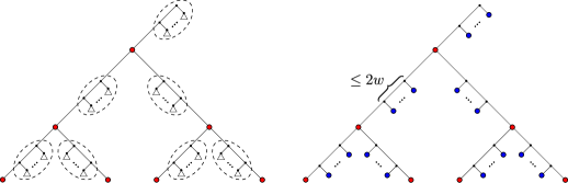
Figure 3: Left: A carving decomposition of the graph $G(\mathcal{N})$ associated with some tensor network $\mathcal{N}$. The red nodes are $Y$-nodes in $\mathit{nodes}(T,Y)$. The nodes inside each dashed region form a connected component $T_{i}$ of the forest $T\backslash\mathit{nodes}(T,Y)$. Right: For each $T_{i}$, let $G[T_{i}]$ be the subgraph of $G(\mathcal{N})$ induced by the vertices $\gamma(\mathit{leaves}(T_{i}))$. Then $G[T_{i}]$ has at most $2w$ connected components $C_{i,j}$. The contraction of all tensors labeling vertices of a component $C_{i,j}$ gives rise to a tensor $g_{i,j}$ of rank at most $2w$. Each such tensor corresponds to a blue node in the carving decomposition to the right.

Lemma 4.12.

$|\mathit{nodes}(T,Y)|=2\cdot|\mathit{leaves}(T,Y)|-1$.

Proof.

Let $u$ be an internal $Y$-node of $T$. We show that $u$ has precisely two $Y$-children. Suppose for contradiction that $u$ has at most one $Y$-child. Then by definition $u$ is not a $Y$-node, since in this case either $\mathit{leaves}(T[u.l],Y)=\emptyset$ or $\mathit{leaves}(T[u.r],Y)=\emptyset$. Now suppose that $u$ has at least $3$ $Y$-children. Since $T$ is a binary tree, two $Y$-children of $u$ are either descendants of $u.l$ or descendants of $u.r$. Lets assume that $z$ and $z^{\prime}$ are two distinct $Y$-children of $u$ which are descendants of $u.l$. We observe that neither $z$ is a descendant of $z^{\prime}$ nor $z^{\prime}$ is a descendant of $z$, since otherwise, only one of these two vertices could have been a $Y$-child of $u$. Now let $u^{\prime}$ be the closest ancestor of $z$ which is also an ancestor of $z^{\prime}$. Then $u^{\prime}$ is by definition a $Y$-node. Since $u^{\prime}$ is a descendant of $u.l$, this contradicts the assumption that $u$ is the $Y$-parent of $z$ and $z^{\prime}$.

Now let $T[Y]$ be the tree whose nodes are $Y$-nodes of $T$ and such that $(u,u^{\prime})$ is an arc of $T[Y]$ if and only if $u$ is the $Y$-parent of $u^{\prime}$. Then by the discussion above we have that $T[Y]$ is a binary tree. Since any binary tree with $|\mathit{leaves}(T,Y)|$ leaves has $|\mathit{leaves}(T,Y)|-1$ internal nodes, the total number of $Y$-nodes in $T$ is $2|Y|-1$ (see Fig. 3). ∎

Now let $T^{\prime}=T\backslash\mathit{nodes}(T,Y)$ be the forest which is obtained by deleting from $T$ all of its $Y$-nodes.

Lemma 4.13.

The number of connected components in the forest $T^{\prime}=T\backslash\mathit{nodes}(T,Y)$ is at most $|\mathit{nodes}(T,Y)|=2|\mathit{leaves}(T,Y)|-1$.

Proof.

Let $T_{1},...,T_{k}$ be the connected components of the forest $T^{\prime}=T\backslash\mathit{nodes}(T,Y)$. For each $i\in\{1,...,k\}$, let $r_{i}$ be the root of $T_{i}$, and let $u_{i}$ be the closest descendant of $r_{i}$ in $T$ which is a $Y$-node. We claim that $u_{i}$ is uniquely determined by $r_{i}$. To see this, assume for the sake of contradiction that there are two descendants $u_{i}$ and $u_{i}^{\prime}$ of $r_{i}$ in $T$ with the property that $u_{i}$ and $u_{i}^{\prime}$ are $Y$-nodes at a minimal distance from $r_{i}$. Let $u_{i}^{\prime\prime}$ be the closest ancestor of $u_{i}$ which is also an ancestor of $u_{i}^{\prime}$. Then $u_{i}^{\prime\prime}$ is by definition a $Y$-node. Since $u_{i}^{\prime\prime}$ is a $Y$-node closer from $r_{i}$ than $u_{i}$ and $u_{i}^{\prime}$, we have reached a contradiction.

Now consider the map $\mu:\{T_{1},...,T_{k}\}\rightarrow\mathit{nodes}(T,Y)$ that sends $T_{i}$ to $\mu(T_{i})=u_{i}$. We claim that the map $\mu$ is an injection, implying in this way that $|\{T_{1},...,T_{k}\}|\leq|\mathit{nodes}(T,Y)|$. Assume for the sake of contradiction that for some $i,j$ with $i\neq j$, $\mu(T_{i})=\mu(T_{j})=u$. Then $u$ is a descendant of $r_{i}$ and a descendant of $r_{j}$ in $T$. This implies that either $r_{i}$ is a descendant of $r_{j}$ in $T$, or $r_{j}$ is a descendant of $r_{i}$ in $T$. Assume that $r_{j}$ is a descendant of $r_{i}$ in $T$. Since by assumption $r_{i}$ and $r_{j}$ belong to distinct connected components in $T\backslash\mathit{nodes}(T,Y)$, there exists at least one $Y$-node $u^{\prime}$ in in the path from $r_{i}$ to $r_{j}$. Therefore, this contradicts the assumption that $u$ is the closest descendant of $r_{i}$ which is a $Y$-node. ∎

Let $T_{1},...,T_{k}$ be the connected components of $T^{\prime}$ where $k\leq|\mathit{nodes}(T,Y)|$. For each $i\in\{1,...,k\}$, let $G[T_{i}]$ be the subgraph of $G(\mathcal{N})$ induced by the vertices $\gamma(\mathit{leaves}(T_{i}))$.

Lemma 4.14.

For each $i\in\{1,...,k\}$, the graph $G[T_{i}]$ has at most $2w$ connected components. Additionally, there are at most $2w$ edges with one endpoint in $G[T_{i}]$ and another endpoint in $G(\mathcal{N})\backslash G[T_{i}]$.

Proof.

Let $r_{i}$ be the root of $T_{i}$ and $u_{i}$ be the closest descendant of $r_{i}$ with the property that $u_{i}$ is a $Y$-node. Since by assumption the carving decomposition $(T,\gamma)$ has width $w$, we have that $|E(V(r_{i}))|\leq w$ and $|E(V(u_{i}))|\leq w$. Suppose for contradiction that the graph $G[T_{i}]$ has at least $2w+1$ connected components. Let $C_{i,1},...,C_{i,c_{i}}$ be the connected components of $G[T_{i}]$, where $c_{i}\geq 2w+1$. Since the graph $G(\mathcal{N})$ is connected, for each $j\in\{1,...,c_{i}\}$ there exists at least one edge with an endpoint in $C_{i,j}$ and another endpoint in $V(u_{i})\cup(V\backslash V(r_{i}))$. This implies that $|E(V(u_{i}))|+|E(V(r_{i}))|\geq 2w+1$, and therefore we have that $|E(V(u_{i}))|\geq w+1$ or $E(V(r_{i}))\geq w+1$. But this contradicts the assumption that the carving-width of $(T,\gamma)$ is at most $w$. Therefore $G(T_{i})$ has at most $2w$ connected components.

The proof of the second statement is also by contradiction. Assume that there are at least $2w+1$ edges with one endpoint in $G[T_{i}]$ and other endpoint in $G(\mathcal{N})\backslash G[T_{i}]$. Since all vertices in $G(\mathcal{N})\backslash G[T_{i}]$ are mapped to leaves in $\mathit{leaves}(T)\backslash\mathit{leaves}(T_{i})$, we have that $|E(V(u_{i}))|+|E(V(r_{i}))|\geq 2w+1$. But then $|E(V(u_{i}))|\geq w+1$ or $|E(V(r_{i}))|\geq w+1$. This contradicts the assumption that the carving width of $(T,\gamma)$ is $w$. ∎

Finally, we are in a position to state and prove the main theorem of this section.

Theorem 4.15 (Tensor Network Reduction).

Let $\mathcal{N}$ be an algebraic tensor network of carving width $w$ and algebraic degree $d$ computing a function $f:\{0,1\}^{Y}\rightarrow\{0,1\}$. Let $l\geq|Y|$ be the number of $Y$-tensors in $\mathcal{N}$. Then $f$ can be computed by a tensor network $\mathcal{N}^{\prime}$ of size at most $4l(w+1)$, rank at most $2w$, and algebraic degree $d$.

Proof.

Let $(T,\gamma)$ be a carving decomposition of $G(\mathcal{N})$ of carving width at most $w$. Let $\{T_{1},...,T_{k}\}$ be the connected components of the forest $T\backslash\mathit{nodes}(T,Y)$. Let $G[T_{i}]$ be the subgraph of $G(\mathcal{N})$ induced by the vertices $\gamma(\mathit{leaves}(T_{i}))$. Finally let $C_{i,1},...,C_{i,c_{i}}$ be the connected components of $G[T_{i}]$. We denote by $\mathcal{N}[Y]$ the set of $Y$-tensors of $\mathcal{N}$. Note that if $g$ is not in $\mathcal{N}[Y]$ then $g$ has algebraic degree $0$ (since no variable in $Y$ occurs in $g$) and labels some vertex of some connected component $C_{i,j}$. Conversely, each tensor labeling a vertex of a connected component $C_{i,j}$ has algebraic degree $0$. For each $i\in\{1,...,k\}$ and each $j\in\{1,...,c_{i}\}$, let $g_{i,j}$ be the tensor obtained by contracting all tensors labeling vertices of the connected component $C_{j,i}$. Note that $g_{i,j}$ has algebraic degree $0$ due to the fact that ${\mathrm{deg}}(\mathit{Contr}(g,g^{\prime}))\leq{\mathrm{deg}}(g)+{\mathrm{deg}}(g^{\prime})$ for any contractible pair of tensors $g,g^{\prime}$ (Observation 4.3). Let

$$\mathcal{N}^{\prime}=\mathcal{N}[Y]\cup\{g_{i,j}\;|\;i\in\{1,...,k\},j\in\{1,...,c_{i}\}\}$$ (2)

be the resulting tensor network. By Lemma 4.13, $k\leq 2\cdot l-1$. By Lemma 4.14, we have that for each $i\in\{1,...,k\}$, $c_{i}\leq 2w$. Then we have that the number of algebraic tensors in $\mathcal{N}^{\prime}$ is at most $l+(2\cdot l-1)\cdot 2w=4lw-2w+l<4l(w+1)$. Since algebraic tensors in $\mathcal{N}[Y]$ did not get involved into any contraction, both the ranks and the algebraic degrees of these algebraic tensors remain unchanged. Therefore, the algebraic degree of the network $\mathcal{N}^{\prime}$ is still $d$. Now the rank of each new tensor $g_{i,j}$ in $\mathcal{N}^{\prime}$ is equal to the number of edges with one endpoint in $G[T_{i}]$ and another endpoint in $G(\mathcal{N})$. By Lemma 4.14 there are at most $2w$ such edges. Therefore, the rank of $g_{i,j}$ is at most $2w$. ∎

5 Number of Functions Computable by Tensor Networks of a Given Size, Rank and Algebraic Degree

Let $Y$ be a set of variables. The main result of this section (Lemma 5.1) establishes an upper bound on the number of Boolean functions computable by a tensor network over $Y$ of size $m$, rank $r$ and algebraic-degree $d$.

Lemma 5.1.

Let $Y$ be a finite set of variables. For each $m,r,d\in{\mathbb{N}}$ there exists at most $\exp(2^{O(r)}\cdot|Y|^{d+1}\cdot m\cdot\log m)$ Boolean functions $g:\{0,1\}^{Y}\rightarrow\{0,1\}$ which can be computed by some algebraic tensor network over $Y$ of size at most $m$, rank at most $r$ and algebraic-degree at most $d$.

We will prove Lemma 5.1 using the connected component counting method, an algebraic geometric technique developed by Warren in [30].

Definition 5.2 (Sign-Assignment).

Let $W$ be a set of variables and let $P=(p_{1},p_{2},...p_{s})$ be a sequence of real polynomials in $\mathbb{R}[W]$. A $(+,-)$-sign assignment for $P$ is a sequence of inequalities $S=(p_{1}\diamond_{1}0,\;p_{2}\diamond_{2}0,\;...,\;p_{s}\diamond_{s}0)$ where for each $i\in\{1,...,s\}$, $\diamond_{i}\in\{<,>\}$.

We say that a $(+,-)$-sign assignment $S=(p_{1}\diamond_{1}0,\;p_{2}\diamond_{2}0,\;...,\;p_{s}\diamond_{s}0)$ is consistent if $S$ is solvable. In other words, $S$ is consistent if there exists an assignment $\beta:W\rightarrow\mathbb{R}$ of the variables in $W$ such that for every $i\in\{1,...,s\}$, the inequality $p_{i}(\beta)\diamond_{i}0$ is satisfied. The following theorem establishes an upper-bound for the number of consistent $(+,-)$-sign assignments for a sequence of polynomials $P$ in terms of three parameters: the number of variables in $W$, the number of polynomials in $P$, and the maximum degree of a polynomial in $P$. Below, $e\approx 2.71$ is the Euler number.

Theorem 5.3 (Warren 1968. Theorem 3 of [30]).

Let $P=(p_{1},p_{2},...,p_{s})$ be real polynomials in $\nu$ variables, each of degree at most $D\geq 1$. If $s\geq\nu$, then the number of consistent $(+,-)$-sign assignments for $P$ is at most $\left(\frac{4\cdot e\cdot D\cdot s}{\nu}\right)^{\nu}$.

Let $\mathcal{N}$ be an algebraic tensor network and let $G(\mathcal{N})=(V,E,\mathbf{g},\eta)$ be the graph associated with $\mathcal{N}$. The type of $\mathcal{N}$ is defined as $\mathit{type}(\mathcal{N})=(V,E)$. In other words, the type of $\mathcal{N}$ is the unlabeled graph obtained from $G(\mathcal{N})$ by forgetting vertex-labels and edge-labels.

Proposition 5.4.

There are at most $m^{r\cdot m}$ types of tensor networks of rank $r$ containing $m$ tensors.

Proof.

Let $\mathcal{N}$ be a tensor of rank $r$ containing $m$ tensors. Then $\mathit{type}(\mathcal{N})$ is a graph with at most $m$ vertices, and degree at most $r$. For each vertex $v$ in such a graph, there are at most $m^{r}$ ways of connecting $v$ to other $r$ vertices. Therefore, there are at most $(m^{r})^{m}=m^{r\cdot m}$ such graphs. ∎

Let $Y$ be a set of variables. We denote by $\mathcal{M}(Y,d)$ the set of monomials in $Y$ of degree at most $d$. Note that $|\mathcal{M}(Y,d)|\leq|Y|^{d}$. Now let $G$ be a fixed type of algebraic tensor network of rank $r$ and size $m$. We will establish an upper bound on the number of functions computable by tensor networks over $Y$ of algebraic-degree $d$ and type $G$. Let $\mathcal{N}=[g_{1},...,g_{m}]$ be such a tensor network. Since $\mathcal{N}$ has algebraic degree $d$, each entry of each algebraic tensor $g_{j}$ in $\mathcal{N}$ is a complex polynomial $p=\sum_{M\in\mathcal{M}(Y,d)}(a_{M}+b_{M}\cdot i)M$ in $Y$ of degree at most $d$, where $a_{M}$ and $b_{M}$ are real numbers. Therefore, each such polynomial can be specified by at most $2\cdot|Y|^{d}$ real numbers. Since $g$ has rank at most $r$, $g_{j}$ has at most $4^{r}$ entries. Finally, $\mathcal{N}$ has $m$ tensors. Therefore, if we let $\mu=4^{r}\cdot m\cdot|Y|^{d}$, the whole tensor network $\mathcal{N}$ can be specified by a sequence of $2\cdot\mu$ real numbers $a_{1},...,a_{\mu},b_{1},...,b_{\mu}$. We let $\mathcal{N}[a_{1},...,a_{\mu},b_{1},...,b_{\mu}]$ be the algebraic tensor network over $Y$ of rank at most $r$, size $m$ and algebraic-degree at most $d$ specified by this sequence.

Now, regard $a_{1},...,a_{\mu},b_{1},...,b_{\mu}$ as real variables. Then each entry of each tensor in the network $\mathcal{N}[a_{1},...,a_{\mu},b_{1},...,b_{\mu}]$ is a complex polynomial $p$ of degree at most $d+1$ in the variables $Y\cup\{a_{1},...,a_{\mu},b_{1},...,b_{\mu}\}$. Additionally, each term of $p$ has a single occurrence of a variable in $\{a_{1},...,a_{\mu},b_{1},...,b_{\mu}\}$. Let $\alpha:Y\rightarrow\{0,1\}$ be a Boolean assignment for the variables $Y$, and let $\mathcal{N}[a_{1},...,a_{\mu},b_{1},...,b_{\mu}](\alpha)$ be the algebraic tensor network obtained by substituting the value $\alpha(x)$ for each variable $x\in Y$ occurring in $\mathcal{N}[a_{1},...,a_{\mu},b_{1},...,b_{\mu}]$. Then $\mathcal{N}[a_{1},...,a_{\mu},b_{1},...,b_{\mu}](\alpha)$ is an algebraic tensor network of over the real variables $\{a_{1},...,a_{\mu},b_{1},...,b_{\mu}\}$ whose algebraic degree is at most $1$. Therefore, the total degree of this network is at most $m$, and by Proposition 4.6, the polynomial

$$p_{\alpha}(a_{1},...,a_{\mu},b_{1},...,b_{\mu})=\mathcal{V}_{\mathcal{N}[a_{1},...,a_{\mu},b_{1},...,b_{\mu}](\alpha)}^{2}$$ (3)

is a real polynomial in $\mathbb{R}[\{a_{1},...,a_{\mu},b_{1},...,b_{\mu}\}]$ of degree at most $2\cdot m$.

Let $h:\{0,1\}^{Y}\rightarrow\{0,1\}$ be a Boolean function on variables $Y$. For each assignment $\alpha\in\{0,1\}^{Y}$, let $\diamond_{\alpha}$ be the greater-than symbol $>$ if $h(\alpha)=1$, and the less-than symbol $<$ if $h(\alpha)=0$. Consider the following system of $2^{|Y|}$ polynomials, indexed by Boolean assignments $\alpha\in\{0,1\}^{Y}$.

$$p_{\alpha}(a_{1},...,a_{\mu},b_{1},...,b_{\mu})-1/4\diamond_{\alpha}0,\hskip 28.45274pt\alpha\in\{0,1\}^{Y}$$ (4)

Assume that $h:\{0,1\}^{Y}\rightarrow\{0,1\}$ is computable by an algebraic tensor network of size $m$, rank $r$, algebraic degree $d$, and type $G$. Then for some real numbers $a_{1}^{h},...,a_{\mu}^{h},b_{1}^{h},...,b_{\mu}^{h}$ the algebraic tensor network $\mathcal{N}_{h}=\mathcal{N}[a_{1}^{h},...,a_{\mu}^{h},b_{1}^{h},...,b_{\mu}^{h}]$ computes $h$. In other words, for each Boolean assignment $\alpha:\{0,1\}^{Y}\rightarrow\{0,1\}$, we have that $\mathcal{V}_{\mathcal{N}_{h}}(\alpha)$ is greater than $1/2$ if $h(\alpha)=1$, and less than $1/2$ if $h(\alpha)=0$. This implies that $p(a_{1}^{h},...,a_{\mu}^{h},b_{1}^{h},...,b_{\mu}^{h})$ is greater than $1/4$ if $h(\alpha)=1$, and less than $1/4$ if $h(\alpha)=0$. Therefore the sequence $a_{1}^{h},...,a_{\mu}^{h},b_{1}^{h},...,b_{\mu}^{h}$ satisfies all inequalities of the system given in Equation 4.

The discussion above shows that the number of Boolean functions computable by an algebraic tensor network over $Y$ of size at most $m$, rank at most $r$, algebraic degree at most $d$, and type $G$ is upper bounded by the number of consistent sign assignments for the system of inequalities of Equation 4. Therefore we can use Theorem 5.3 to estimate this number. By setting $s=2^{|Y|}$, $\nu=2\mu=2\cdot 4^{r}\cdot m\cdot|Y|^{d}$, and $D=2m$ in Theorem 5.3 we have that the number of consistent assignments for the system of polynomials in Equation 4 is at most

$$\left(\frac{4\cdot e\cdot(2m)\cdot 2^{|Y|}}{2\cdot 4^{r}\cdot m\cdot|Y|^{d+1}}\right)^{2\cdot 4^{r}\cdot m\cdot|Y|^{d}}\leq\exp(2^{O(r)}\cdot|Y|^{d+1}\cdot m).$$

Therefore, there are at most $\exp(2^{O(r)}\cdot|Y|^{d+1}\cdot m)$ functions computable by some tensor network over $Y$ of algebraic degree at most $d$, with type $G$. Since, by Proposition 5.4, there are at most $m^{r\cdot m}\leq\exp(O(r\cdot m\cdot\log m))$ types of network of rank $r$ and size $m$, we have that the total number of functions computable by an algebraic tensor network over $Y$ of algebraic-degree $d$, rank $r$ and size $m$ is upper bounded by

$$\exp(2^{O(r)}\cdot|Y|^{d+1}\cdot m+O(r\cdot m\cdot\log m))\leq\exp(2^{O(r)}\cdot|Y|^{d+1}\cdot m\cdot\log m).$$

This proves Lemma 5.1. $\square$

6 Upper Bounding the Number of Subfunctions of a Function

Let $X=\{x_{1},...,x_{n}\}$ be a set of variables, $f:\{0,1\}^{X}\rightarrow\{0,1\}$ be a Boolean function on $X$, and $Y\subseteq X$ be a subset of variables of $X$. We denote by $N_{f}(Y)$ the number of distinct functions obtained from $f$ by initializing all variables in $X\backslash Y$ with values in $\{0,1\}$. Now assume that $f$ is computed by an algebraic tensor network $\mathcal{N}$. The next theorem establishes an upper bound for $N_{f}(Y)$ in terms of number of $Y$-tensors in $\mathcal{N}$, and in terms of the treewidth, rank and algebraic degree of $\mathcal{N}$.

Theorem 6.1 (Main Technical Theorem).

Let $f:\{0,1\}^{X}\rightarrow\{0,1\}$ be a function computable by an algebraic tensor network $\mathcal{N}$ of treewidth $t$, rank $k$, and algebraic-degree $d$. Let $Y\subseteq X$, and $l$ be the number of $Y$-tensors in $\mathcal{N}$. Then $N_{f}(Y)$ is at most $\exp\left(2^{O(r\cdot t)}\cdot|Y|^{d+1}\cdot l\cdot\log l\right)$.

Proof.

Let $f:\{0,1\}^{X}\rightarrow\{0,1\}$ be a function computable by an algebraic tensor network $\mathcal{N}$ over $X$ of rank $r$ and algebraic-degree $d$. Since $G(\mathcal{N})$ has treewidth $t$ and maximum (vertex) degree $r$, Lemma 4.10 implies that the carving width of $G(\mathcal{N})$ is at most $w=O(r\cdot t)$.

Let $Y\subseteq X$, and $l$ be the number of $Y$-tensors in $\mathcal{N}$. Let $\beta:\{0,1\}^{X\backslash Y}\rightarrow\{0,1\}$ be an assignment of the variables in $X\backslash Y$, and let $\mathcal{N}(\beta)$ be the algebraic tensor network over $Y$, obtained by initializing the variables in $X\backslash Y$ according to the assignment $\beta$. Then $\mathcal{N}(\beta)$ computes the function $g:\{0,1\}^{Y}\rightarrow\{0,1\}$ which is obtained from $f$ by restricting the variables in $X\backslash Y$ according to $\beta$.

By Theorem 4.15, the function $g$ can be computed by an algebraic tensor network $\mathcal{N}^{\prime}$ over $Y$ of algebraic degree $d$, rank $r^{\prime}=O(r\cdot t)$, and size $m=O(r\cdot t\cdot l)$. Therefore, by Lemma 5.1 we have that there exist at most

$$\exp\left(2^{O(r\cdot t)}\cdot|Y|^{d+1}\cdot O(r\cdot t\cdot l\cdot\log(r\cdot t\cdot l))\right)=\exp\left(2^{O(r\cdot t)}\cdot|Y|^{d+1}\cdot l\cdot\log l\right)$$

Boolean functions $g:\{0,1\}^{Y}\rightarrow\{0,1\}$ which can be obtained from $f$ by initializing the variables in $X\backslash Y$ with elements from $\{0,1\}$. ∎

7 Quadratic Lower Bounds For Algebraic Networks and Quantum Circuits of Constant Treewidth

Let $X=\{x_{1},...,x_{n}\}$ be a set of $n=2k\log k$ distinct variables partitioned into $k$ blocks $Y_{1},Y_{2},...,Y_{k}$, where each block $Y_{i}$ has $2\log k$ variables. The element distinctness function $\delta_{n}:\{0,1\}^{X}\rightarrow\{0,1\}$ is defined as follows for each assignment $s_{1},s_{2},...,s_{k}$ of the blocks $Y_{1},Y_{2},...,Y_{k}$ respectively.

$$\delta_{n}(s_{1},s_{2},...,s_{k})=\left\{\begin{array}[]{lll}1&&\mbox{if $s_{i}\neq s_{j}$ for $i\neq j$},\\ 0&&\mbox{otherwise.}\end{array}\right.$$ (5)

The following lemma states that the element distinctness function defined in Equation 5 has many sub-functions.

Lemma 7.1 ([19], Section 6.5).

Let $\delta_{n}:\{0,1\}^{X}\rightarrow\{0,1\}$ be the element distinctness function defined in Equation 5, where $|X|=n$ and $X=Y_{1}\;\dot{\cup}\;Y_{2}\;\dot{\cup}...\;\dot{\cup}\;Y_{k}$ with $|Y_{i}|=2\log k$. Then for each $i\in\{1,...,k\}$, $N_{\delta_{n}}(Y_{i})\geq 2^{\Omega(n)}$.

The following theorem follows as a combination of Theorem 6.1 and Lemma 7.1.

Theorem 7.2.

Let $X$ be a set with $n$ Boolean variables, and let $\delta_{n}:\{0,1\}^{X}\rightarrow\{0,1\}$ be the $n$-bit element distinctness function. Let $\mathcal{N}$ be a tensor network of treewidth $t$, rank $r$ and algebraic degree $d$ computing $\delta_{n}$. Then $\mathcal{N}$ has size

$$\Omega\left(\frac{n^{2}}{2^{O(r\cdot t)}\cdot(\log n)^{d+3}}\right).$$

Proof.

For each $i\in\{1,...,k\}$ let $l_{i}$ be the number of $Y_{i}$-nodes in $\mathcal{N}$ where $Y_{i}$ is the $i$-th block of variables. If $l_{i}\geq n^{2}$, then the theorem is true and there is nothing to be proved. Therefore, assume that $l_{i}<n^{2}$, and hence that $\log l_{i}<2\log n$. For each $i\in\{1,...,k\}$, by plugging $l_{i}$ and $|Y_{i}|=2\log n$ in Theorem 6.1, we have that

$$N_{\delta_{n}}(Y_{i})\leq\exp\left(2^{O(r\cdot t)}\cdot(\log n)^{d+1}\cdot l_{i}\cdot\log l_{i}\right)\leq\exp\left(2^{O(r\cdot t)}\cdot(\log n)^{d+2}\cdot l_{i}\right).$$ (6)

Now, by Lemma 7.1, we have that $N_{\delta_{n}}(Y_{i})\geq 2^{\Omega(n)}$, and therefore,

$$\exp\left(2^{O(r\cdot t)}\cdot(\log n)^{d+2}\cdot l_{i}\right)\geq N_{\delta_{n}}(Y_{i})\geq 2^{\Omega(n)}.$$ (7)

Equation 7 implies that

$$l_{i}\geq\Omega\left(\frac{n}{2^{O(r\cdot t)}\cdot(\log n)^{d+2}}\right).$$

Since there are $k=\Omega(\frac{n}{\log n})$ blocks of variables $Y_{i}$, we have that the total number of tensors in $\mathcal{N}$, which is greater than $\sum_{i}l_{i}$, is at least

$$\Omega\left(\frac{n^{2}}{2^{O(r\cdot t)}\cdot(\log n)^{d+3}}\right).$$

∎

Finally, our main theorem follows as a corollary of Theorem 7.2.

Theorem 7.3 (Main Theorem).

Let $X$ be a set with $n$ Boolean variables, and let $\delta_{n}:\{0,1\}^{X}\rightarrow\{0,1\}$ be the $n$-bit element distinctness function. Let $C$ be a quantum circuit over $X$ computing $\delta_{n}$. If $C$ has treewidth $t$ and all gates in $C$ act on at most $r$ qubits, then $C$ has at least $\Omega\left(\frac{n^{2}}{2^{O(r\cdot t)}\cdot(\log n)^{4}}\right)$ gates.

Proof.

Let $\mathcal{N}_{C}$ be the algebraic tensor network associated with $C$. Then $\mathcal{N}_{C}$ has algebraic degree $1$, treewidth $t$, and rank at most $2\cdot r$. By Theorem 7.2, $\mathcal{N}_{C}$ must have at least $\Omega\left(\frac{n^{2}}{2^{O(r\cdot t)}\cdot(\log n)^{4}}\right)$ tensors, and therefore $C$ must have at least this number of gates. ∎

8 Final Comments and Open Problems

In this work we have shown that any quantum circuit of treewidth at most $t$, build up from $r$-qubit gates, requires at least $\Omega(n^{2}/2^{O(r\cdot t)}\log^{4}n)$ gates to compute the element distinctness function $\delta_{n}:\{0,1\}^{n}\rightarrow\{0,1\}$ (Theorem 7.3). This lower bound is robust for three reasons. First, it does not assume that the quantum gates belong to any particular finite basis. The only requirement is that these gates act on at most $r$ qubits. Second, we do not assume any upper bound on the number of bits necessary to represent each entry of such a gate. Third, we consider that a function $f:\{0,1\}^{X}\rightarrow\{0,1\}$ is computed by a quantum circuit $C$ if the acceptance probability of $C$ on input $\alpha\in\{0,1\}^{X}$ is greater than $1/2$ whenever $f(\alpha)=1$, and less than $1/2$ whenever $f(\alpha)=0$. Thus we assume no gap between the acceptance and rejection probabilities for a given input $\alpha$.

There are many interesting open problems concerning circuits of constant treewidth. For instance, can quantum circuits of treewidth $t$ be polynomially simulated by quantum (or classical) circuits of treewidth $t-1$? Can quantum circuits of treewidth $t$ be polynomially simulated by quantum formulas (i.e. quantum circuits of treewidth $1$)? Also, we should mention the longstanding open problem of determining whether quantum formulas can be polynomially simulated by classical formulas [27]. Progress towards this question has only been made in the read-once setting. More precisely, it has been shown that read-once quantum formulas can be polynomially simulated by classical formulas of same size built from Toffoli and NOT gates [7]. Nevertheless this simulation breaks down if the read-once condition is removed [7]. It would be interesting to determine whether a similar result can be achieved for read-once quantum circuits of constant treewidth. Can read-once quantum circuits of treewidth $t$ be polynomially simulated by read-once classical circuits of treewidth $t$?

8.1 Acknowledgements

The author thanks Christian Komusiewicz for valuable comments and suggestions. The author acknowledges support from the Bergen Research Foundation. Part of this work was done while the author was at the Czech Academy of Sciences, supported by the European Research Council (grant number 339691).

Appendix A Proof of Proposition 4.8

In this section we show that any quantum circuit $C$ with $m$ gates, treewidth $t$, build from $r$-qubit gates, can be simulated by an algebraic tensor network $\mathcal{N}_{C}$ with $m$ algebraic tensors, treewidth $t$, rank $2r$, and algebraic degree $1$. The construction of $\mathcal{N}_{C}$ from $C$ is based on a construction given in [21] which converts quantum circuits in which all inputs are initialized to tensor networks (i.e. algebraic tensor networks of degree $0$). Below, we modify this construction to take into consideration input vertices that are are labeled with variables.

Let $C=(V,E,{\theta},{\xi})$ be a quantum circuit over a set of variables $X$. The tensor network $\mathcal{N}_{C}$ is obtained by creating a tensor $g_{v}$ for each vertex $v\in V$.

Let $v$ be an internal vertex of $C$ whose incoming edges are labeled with numbers $\{i_{1},...,i_{k}\}$ and outgoing edges are labeled with numbers $\{j_{1},...,j_{k}\}$. Let $v$ be labeled with a unitary matrix $U\in{\mathbb{C}}^{2^{k}\times 2^{k}}$. Then the tensor $g_{v}$ has index set $\{i_{1},...,i_{k},j_{1},...,j_{k}\}$, and the value of $g_{v}$ on each entry $\sigma_{i_{1}},...,\sigma_{i_{k}},\sigma_{j_{1}},...,\sigma_{j_{k}}\in\Pi^{2k}$ is defined as follows.

$$g_{v}(\sigma_{i_{1}},...,\sigma_{i_{k}},\sigma_{j_{1}},...,\sigma_{j_{l}})={\mathit{Tr}}\left([\sigma_{j_{1}}^{\dagger}\otimes...\otimes\sigma_{j_{l}}^{\dagger}]\cdot U\cdot[\sigma_{i_{1}}\otimes...\otimes\sigma_{i_{k}}]\right).$$ (8)

Let $v$ be an output vertex whose unique incoming edge is labeled with number $j$. Let $v$ be labeled with a $1$-qubit measurement element $M$ in ${\mathbb{C}}^{2\times 2}$. Then the tensor $g_{v}$ has index set $\{j\}$, and the value of $g_{v}$ on each entry $\sigma_{j}\in\Pi$ is defined as follows.

$$g_{v}(\sigma_{j})={\mathit{Tr}}\left(\sigma_{j}^{\dagger}\cdot M\right).$$ (9)

For each variable $x$ we define the following matrix: $|x\rangle\langle x|=\left[\begin{array}[]{cc}(1-x)&0\\ 0&x\\ \end{array}\right]$. If $v$ is an input vertex of $C$ whose unique outgoing edge is labeled with number $i$, then we the tensor $g_{v}$ has index set $i$, and the value of $g_{v}$ on each entry $\sigma_{i}\in\Pi$ is defined as follows.

$$g_{v}(\sigma_{i})={\mathit{Tr}}\left(|x\rangle\langle x|\cdot\sigma_{i}\right).$$ (10)

Note that the tensor $g_{v}$ has algebraic degree $1$. On the other hand if such an input vertex $v$ is labeled with a qubit $|b\rangle\in\{|0\rangle,|1\rangle\}$, then the value of $g_{v}$ on each entry $\sigma_{i}\in\Pi$ is defined as.

$$g_{v}(\sigma_{i})={\mathit{Tr}}\left(|b\rangle\langle b|\cdot\sigma_{i}\right).$$ (11)

We note that if all gates in $C$ act on at most $k$ qubits, then the tensor network $\mathcal{N}_{C}$ has rank at most $2k$. Additionally, the graph $G(\mathcal{N})$ is isomorphic to the graph $G(C)$. Therefore, if $C$ has treewidth $t$, then $G(C)$ has also treewidth $t$. We also note tensors associated with input nodes of $C$ labeled with variables have algebraic degree $1$. All other tensors have algebraic degree $0$. Therefore, $\mathcal{N}_{C}$ has algebraic degree $1$. $\square$

References

• [1] M.Β Alekhnovich and A.Β A. Razborov. Satisfiability, branch-width and tseitin tautologies. In Proc. of the 43rd Symposium on Foundations of Computer Science, pages 593–603, 2002.
• [2] E.Β Allender, S.Β Chen, T.Β Lou, P.Β A. Papakonstantinou, and B.Β Tang. Width-parametrized SAT: Time–space tradeoffs. Theory of Computing, 10(12):297–339, 2014.
• [3] S.Β Arnborg, J.Β Lagergren, and D.Β Seese. Easy problems for tree-decomposable graphs. J. Algorithms, 12(2):308–340, 1991.
• [4] S.Β Arnborg and A.Β Proskurowski. Linear time algorithms for NP-hard problems restricted to partial $k$-trees. Discrete Applied Mathematics, 23(1):11–24, 1989.
• [5] E.Β Broering and S.Β V. Lokam. Width-based algorithms for SAT and CIRCUIT-SAT. In Theory and Applications of Satisfiability Testing, pages 162–171. Springer, 2004.
• [6] C.Β Calabro. A lower bound on the size of series-parallel graphs dense in long paths. In Electronic Colloquium on Computational Complexity (ECCC), Tech report TR08-110, 2008. http://eccc.hpi-web.de/eccc.
• [7] A.Β Cosentino, R.Β Kothari, and A.Β Paetznick. Dequantizing read-once quantum formulas. In Proc. of the 8th Conference on the Theory of Quantum Computation, Communication and Cryptography (TQC 2013), volumeΒ 22 of LIPIcs, pages 80–92, 2013.
• [8] B.Β Courcelle. The monadic second-order logic of graphs. i. recognizable sets of finite graphs. Information and computation, 85(1):12–75, 1990.
• [9] M.Β deΒ OliveiraΒ Oliveira. On the satisfiability of quantum circuits of small treewidth. In Proc. of the 10th International Computer Science Symposium in Russia (CSR 2015), volume 9139 of LNCS, pages 157–172, 2015.
• [10] M.Β deΒ OliveiraΒ Oliveira. Size-Treewidth Tradeoffs for Circuits Computing the Element Distinctness Function. In Proc. of the 33rd Symposium on Theoretical Aspects of Computer Science (STACS 2016), volumeΒ 47 of LIPIcs, pages 56:1–56:14, 2016.
• [11] E.Β D. Demaine, F.Β V. Fomin, M.Β T. Hajiaghayi, and D.Β M. Thilikos. Subexponential parameterized algorithms on bounded-genus graphs and H-minor-free graphs. J. ACM, 52(6):866–893, 2005.
• [12] M.Β G. Find, A.Β Golovnev, E.Β A. Hirsch, and A.Β S. Kulikov. A better-than-3n lower bound for the circuit complexity of an explicit function. Electronic Colloquium on Computational Complexity (ECCC), 22:166, 2015.
• [13] A.Β GΓ‘l and J.-T. Jang. A generalization of spira’s theorem and circuits with small segregators or separators. In SOFSEM 2012: Theory and Practice of Computer Science, pages 264–276. Springer, 2012.
• [14] K.Β Georgiou and P.Β A. Papakonstantinou. Complexity and algorithms for well-structured k-sat instances. In Proc. of the 11th International Conference on Theory and Applications of Satisfiability Testing, pages 105–118. Springer, 2008.
• [15] J.Β HΓ₯stad. The shrinkage exponent of de morgan formulas is 2. SIAM Journal on Computing, 27(1):48–64, 1998.
• [16] J.Β He, H.Β Liang, and J.Β M. Sarma. Limiting negations in bounded treewidth and upward planar circuits. In Mathematical Foundations of Computer Science 2010, pages 417–428. Springer, 2010.
• [17] K.Β Iwama and H.Β Morizumi. An explicit lower bound of 5n- o (n) for boolean circuits. In Mathematical foundations of computer science 2002, pages 353–364. Springer, 2002.
• [18] M.Β Jansen and J.Β Sarma. Balancing bounded treewidth circuits. In Computer Science–Theory and Applications, pages 228–239. Springer, 2010.
• [19] S.Β Jukna. Boolean function complexity: advances and frontiers, volumeΒ 27. Springer Science & Business Media, 2012.
• [20] O.Β Lachish and R.Β Raz. Explicit lower bound of 4.5 n-o (n) for boolena circuits. In Proceedings of the thirty-third annual ACM symposium on Theory of computing, pages 399–408. ACM, 2001.
• [21] I.Β L. Markov and Y.Β Shi. Simulating quantum computation by contracting tensor networks. SIAM Journal on Computing, 38(3):963–981, 2008.
• [22] Nečiporuk. On a Boolean function. Soviet Math. Dokl., 7(4):999–1000, 1966.
• [23] M.Β A. Nielsen and I.Β L. Chuang. Quantum computation and quantum information. Cambridge university press, 2010.
• [24] R.Β OrΓΊs. A practical introduction to tensor networks: Matrix product states and projected entangled pair states. Annals of Physics, 349:117–158, 2014.
• [25] N.Β Robertson and P.Β D. Seymour. Graph minors. iii. planar tree-width. Journal of Combinatorial Theory, Series B, 36(1):49–64, 1984.
• [26] N.Β Robertson and P.Β D. Seymour. Graph minors. xiii. the disjoint paths problem. Journal of Combinatorial Theory, Series B, 63(1):65–110, 1995.
• [27] V.Β P. Roychowdhury and F.Β Vatan. Quantum formulas: A lower bound and simulation. SIAM Journal on Computing, 31(2):460–476, 2001.
• [28] G.Β TurΓ‘n and F.Β Vatan. On the computation of boolean functions by analog circuits of bounded fan-in. Journal of Computer and System Sciences, 1(54):199–212, 1997.
• [29] L.Β G. Valiant. Graph-theoretic arguments in low-level complexity. In 6th Symposium on Mathematical Foundations of Computer Science, pages 162–176, 1977.
• [30] H.Β E. Warren. Lower bounds for approximation by nonlinear manifolds. Transactions of the American Mathematical Society, pages 167–178, 1968.
• [31] A.Β C.-C. Yao. Quantum circuit complexity. In 34th Annual Symposium on Foundations of Computer Science (Palo Alto, CA, 1993), pages 352–361. IEEE Comput. Soc. Press, Los Alamitos, CA, 1993.