Nonlinear localized flatband modes with spin-orbit coupling

Abstract

We report the coexistence and properties of stable compact localized states (CLSs) and discrete solitons (DSs) for nonlinear spinor waves on a flatband network with spin-orbit coupling (SOC). The system can be implemented by means of a binary Bose-Einstein condensate loaded in the corresponding optical lattice. In the linear limit, the SOC opens a minigap between flat and dispersive bands in the system’s bandgap structure, and preserves the existence of CLSs at the flatband frequency, simultaneously lowering their symmetry. Adding onsite cubic nonlinearity, the CLSs persist and remain available in an exact analytical form, with frequencies which are smoothly tuned into the minigap. Inside of the minigap, the CLS and DS families are stable in narrow areas adjacent to the FB. Deep inside the semi-infinite gap, both the CLSs and DSs are stable too.

I Introduction

Wave dynamics can be tailored by symmetries and topologies imprinted by dint of underlying periodic potentials. In turn, the symmetries and topologies of the periodic potentials can be probed by excitations in the system into which the potential is embedded. In particular, flatband (FB) lattices, existing due to specific local symmetries, provide the framework supporting completely dispersionless bands in the system’s spectrum richter15 . FB lattices have been realized in photonic waveguide arrays guzman-silva14 , exciton-polariton condensates masumoto12 , and atomic Bose-Einstein condensates (BECs) taie15 .

FB lattices are characterized by the existence of compact localized states (CLSs), which, being FB eigenstates, have nonzero amplitudes only on a finite number of sites richter15 . The CLSs are natural states for the consideration of their perturbed evolution. They feature different local symmetry and topology properties, and can be classified according to the number $U$ of unit cells which they occupy flach14 . Perturbations may hybridize CLSs with dispersive states through a spatially local resonant scenario flach14 , similar to Fano resonances miroshnichenko10 . The CLS existence has been experimentally probed in the same settings where FB lattices may be realized, as mentioned above: waveguiding arrays vicencio15 ; mukherjee15 ; weimann16 , exciton-polariton condensates baboux16 , and atomic BECs taie15 . The impact of various perturbations, such as disorder flach14 ; leykam16 , correlated potentials bodyfelt14 ; danieli15 , and external magnetic and electric fields khomeriki16 , on FB lattices and the corresponding CLSs was studied too.

A particularly complex situation arises in the case of much less studied nonlinear perturbations, which can preserve or destroy CLSs, and detune their frequency vicencio13 ; leykam13 ; johannson15 ; lopez-gonzalez16 . Here we study the existence of nonlinear localized modes in a pseudospinor (two-component) diamond chain, whose components are linearly mixed due to spin-orbit-coupling (SOC). The system can be implemented using a binary Bose-Einstein condensate (BEC) trapped in an optically imprinted potential emulating, e.g., the ”diamond chain” flach14 . The two components represent different atomic states, and the SOC interaction between them can be induced by means of a recently elaborated technique, making use of properly applied external magnetic and optical fields SOC . The possibility to model these settings by discrete dynamics in a deep optical-lattice potential was demonstrated, in a general form, in Refs. discreteso ; nashsoc . We consider two types of nonlinearities produced by interactions between atoms in the BEC, viz., intra- and inter-component ones. The main objective of the analysis is to analyze the impact of the SOC on the linear and nonlinear CLS modes, as well as on exponentially localized discrete solitons. We demonstrate the possibility to create diverse stable localized modes at and close to the FB frequency, and inside gaps opened by the SOC.

In a previous work nashsoc , we studied the effect of the SOC on the dynamics of discrete solitons in a binary BEC trapped in a deep one-dimensional (1D) optical lattice. Among new findings related to the SOC were the tunability of the transition between different types of localized complexes, provided by the SOC strength, and the opening of a minigap in the spectrum induced by the SOC. Inside the minigap, miscible stable on-site soliton complexes were found nashsoc . In the opposite, quasi-continuum limit, one- and two-dimensional discrete solitons supported by the SOC were studied too discreteso .

The paper is structured as follows. The model is introduced in Section II. Following a brief recapitulation of the spectral properties of the single-component linear quasi-1D diamond-chain lattice, the two-component system is considered. It is shown that the SOC opens gaps between the FBs and DBs in the spectrum. In Section III, exact solutions for CLS modes are constructed in the linear system with the SOC terms. Effects of the SOC on nonlinear CLS modes, and a possibility to create other types of the localized ones, in gaps between the FB and DB is considered in Section IV. In particular, the nonlinear CLSs are found in an exact analytical form too. In that Section, localized modes in the semi-infinite gap (SIG) are briefly considered too. The paper is concluded by Section V.

II Model equations

II.1 The single-component model

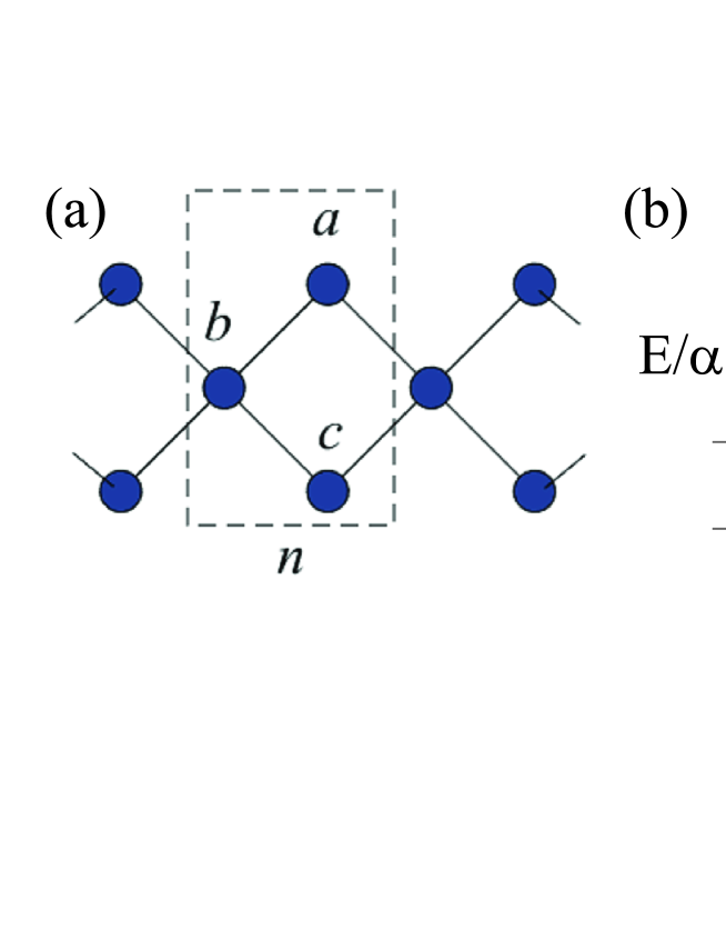
Figure 1: (a) The schematic of the diamond chain corresponding to Eq. (1). Circles and solid lines designate lattice sites, and hoppings, respectively. The dashed rectangle defines the unit cell, consisting of a (upper), b (middle) and c (bottom) sites. (b) The dispersion relation for the linear case $\beta=0$ (see details in the text).

We consider the one-dimensional ”diamond-chain” lattice shown in Fig. 1(a). Its bandgap structure, shown in Fig. 1(b), consists of two DBs which merge with the FB at conical intersection point located at the edge of the Brillouin zone flach14 . The tight-binding (discrete) model governing the propagation of waves through this system is based on the following equations:

$$i\frac{da_{n}}{dt}+\alpha(b_{n}+b_{n+1})+\beta|a_{n}|^{2}a_{n}=0,$$

$$i\frac{db_{n}}{dt}+\alpha(a_{n}+a_{n-1}+c_{n}+c_{n-1})+\beta|b_{n}|^{2}b_{n}=0,$$ (1)

$$i\frac{dc_{n}}{dt}+\alpha(b_{n}+b_{n+1})+\beta|c_{n}|^{2}c_{n}=0,$$

where $\alpha$ is the nearest-neighbor coupling strength and $\beta$ the nonlinearity coefficient. These discrete Gross-Pitaevskii equations (GPEs) describe a BEC trapped in the deep optical lattice. The same system can be realized in optics, as an array of transversely coupled waveguides. In that case, time $t$ is replaced by the propagation distance $z$. The evolution equations (1) can be derived from the Hamiltonian

$$\mathcal{H}=\sum_{n}\left\{\epsilon_{a,n}|a_{n}|^{2}+\epsilon_{b,n}|b_{n}|^{2}+\epsilon_{c,n}|c_{n}|^{2}+\frac{\beta}{2}(|a_{n}|^{4}\right.$$ (2)

$$\left.+|b_{n}|^{4}+|c_{n}|^{4})+\alpha\left[(a_{n}^{\ast}+c_{n}^{\ast})(b_{n}+b_{n+1})+\mathrm{c.c.}\right]\right\},$$ (3)

which is conserved, along with the norm, $N=\sum_{n}(|a_{n}|^{2}+|b_{n}|^{2}+|c_{n}|^{2})$.

In the linear limit, $\beta=0$, the modal profiles, $\mathbf{\psi}_{n}=\{a_{n},b_{n},c_{n}\}$ are looked for as

$$\{{a}_{n}(t),{b}_{n}(t),{c}_{n}(t)\}=\mathbf{\Psi}_{n}e^{-iEt}.$$ (4)

Using the Bloch basis, $\mathbf{\Psi}_{n}=\mathbf{\Psi}e^{ikn}$, with wavenumber $k$ and the polarization eigenvectors

$$\mathbf{\Psi}^{(0)}=\frac{1}{\sqrt{2}}(1,0,-1),\mathbf{\Psi}^{(\pm)}=\frac{1}{2}\left(1,\pm\frac{1+e^{ik}}{\sqrt{1+\cos k}},1\right),$$ (5)

we obtain the band structure which consists of three branches

$$E_{\mathrm{FB}}(k)=0\;,\;E_{\pm}(k)=\pm 2\sqrt{2}\alpha\cos(k/2).$$ (6)

Two DBs are $k$-dependent branches, and the $k$-independent one is the FB, see Fig. 1(b).

Henceforth, we set $\alpha=1$, by means of rescaling. The FB states with $E=0$ in Eq. (5) are independent of $k$, and may be perfectly localized in a single cell in the form of the linear CLS flach14 ,

$$\mathbf{\Psi}_{n}=\delta_{n,n_{0}}\mathbf{\Psi}^{(0)}\equiv\delta_{n,n_{0}}\frac{1}{\sqrt{2}}(1,0,-1),$$ (7)

where $\delta_{i,j}$ is the Kronecker’s symbol, and $n_{0}$ determines the location of the cell. Diffractive decay of the CLS is prevented by the opposite signs of the field amplitudes at sites $a$ and $c$ and the corresponding destructive interference.

The CLSs are, strictly speaking, infinitely degenerate states, as they can be positioned in any unit cell. Any superposition of CLSs eigenvectors is also an eigenvector. The present CLS belongs to class $U=1$, as it occupies only one unit cell.

II.2 The two-component system

The basic model in our study is a two-component (pseudospinor) system carried by the diamond chain, with the (pseudo-) SOC of strength $\lambda$ which induces the linear mixing between the two components, following the lines of Ref. discreteso (where the SOC of the Rashba type SOC was adopted). The components represent two hyperfine states of the same atomic species in the binary BEC. One can think of the diamond chain as a stripe embedded into a two-dimensional network, with the wave functions vanishing at all other sites. The anisotropy of the SOC defines a direction which forms some angle with the diamond-chain’s axis connecting all $b$ sites. Below we set this angle to be $\pi/4$, although the cases of $0$ or $\pi/2$, as well as the general case of an arbitrary angle can be readily considered as well. Thus, the positive $x$-axis is directed from site $b$ to $c$ in a unit cell, and the positive $y$-axis from $b$ to $a$ in the same cell. The two different components of the discrete wave functions are denoted $a_{n}^{\pm},b_{n}^{\pm},c_{n}^{\pm}$. We can also add a (pseudo) magnetic field $B$ which induces a Zeeman splitting, in terms of SOC. The corresponding system of discrete GPEs is

$$i\frac{da_{n}^{+}}{dt}+Ba_{n}^{+}+b_{n}^{+}+b_{n+1}^{+}+\lambda\left(b_{n+1}^{-}+ib_{n}^{-}\right)+(\gamma|a_{n}^{+}|^{2}+\zeta|a_{n}^{-}|^{2})a_{n}^{+}=0,$$

$$i\frac{db_{n}^{+}}{dt}+Bb_{n}^{+}+a_{n}^{+}+a_{n-1}^{+}+c_{n}^{+}+c_{n-1}^{+}+\lambda\left[c_{n}^{-}-a_{n-1}^{-}-i(a_{n}^{-}-c_{n-1}^{-})\right]+(\gamma|b_{n}^{+}|^{2}+\zeta|b_{n}^{-}|^{2})b_{n}^{+}=0,$$

$$i\frac{dc_{n}^{+}}{dt}+Bc_{n}^{+}+b_{n}^{+}+b_{n+1}^{+}-\lambda\left(b_{n}^{-}+ib_{n+1}^{-}\right)+(\gamma|c_{n}^{+}|^{2}+\zeta|c_{n}^{-}|^{2})c_{n}^{+}=0,$$

$$i\frac{da_{n}^{-}}{dt}-Ba_{n}^{-}+b_{n}^{-}+b_{n+1}^{-}-\lambda\left(b_{n+1}^{+}-ib_{n}^{+}\right)+(\gamma_{1}|a_{n}^{-}|^{2}+\zeta|a_{n}^{+}|^{2})a_{n}^{-}=0,$$

$$i\frac{db_{n}^{-}}{dt}-Bb_{n}+a_{n}^{-}+a_{n-1}^{-}+c_{n}^{-}+c_{n-1}^{-}-\lambda\left[c_{n}^{+}-a_{n-1}^{+}+i(a_{n}^{+}-c_{n-1}^{+})\right]+(\gamma_{1}|b_{n}^{-}|^{2}+\zeta|b_{n}^{+}|^{2})b_{n}^{-}=0,$$

$$i\frac{dc_{n}^{-}}{dt}-Bc_{n}^{-}+b_{n}^{-}+b_{n+1}^{-}+\lambda\left(b_{n}^{+}-ib_{n+1}^{+}\right)+(\gamma_{1}|c_{n}^{-}|^{2}+\zeta|c_{n}^{+}|^{2})c_{n}^{-}=0,$$ (8)

where two types of the local nonlinear terms are included: collisions between atoms belonging to the same component generate the cubic self-interaction with coefficients $\gamma$ and $\gamma_{1}$ in Eq. (8), while collisions between atoms from different components give rise to the cross-interaction accounted for by coefficient $\zeta$.

The above set of equations is invariant under the symmetry operation, which involves the permutation of the SOC components, simultaneous sign change of the magnetic field, the complex conjugation, and time reversal:

$$\{a,b,c\}^{\pm}\rightarrow\{a^{\ast},b^{\ast},c^{\ast}\}^{\mp}\;,\;B\rightarrow-B\;,\;t\rightarrow-t\;.$$ (9)

Note that in the nonlinear case this symmetry holds only if $\gamma=\gamma_{1}=\zeta$.

The linear system with $\gamma=\gamma_{1}=\zeta=0$ and in the absence of the SOC and magnetic fields, $\lambda=B=0$, is characterized by a double-degenerate single-component spectrum of the diamond chain from the previous section. Therefore, the FB exists and is double degenerate too, due to the presence of two pseudospin components. For $\lambda=0$ but $B\neq 0$, the spectrum of each component is shifted by $\pm B$ relative to the single-component model outlined in the previous section, see Fig. 2 (a). Thus, both FBs survive, but their degeneracy is lifted. When the SOC is present, $\lambda\neq 0$, together with the Zeeman terms, the FBs are deformed (made dispersive), losing the flatness, see Fig. 2(b-d).

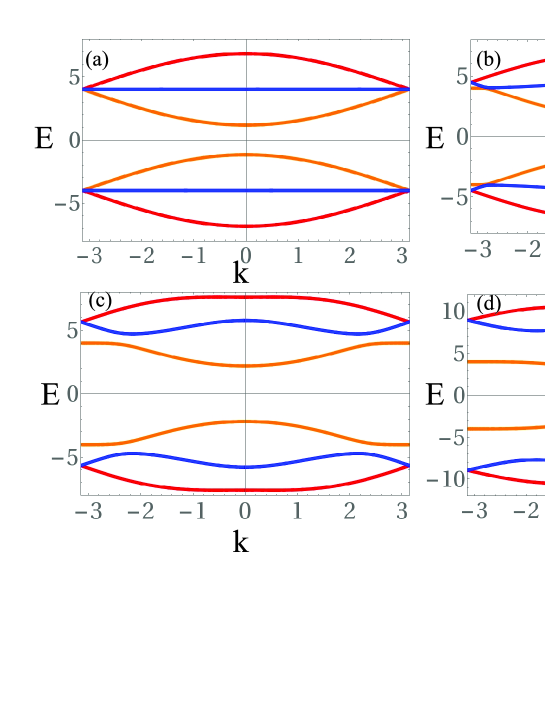
Figure 2: Dispersion relations for the two-component system with $B=4$ and (a) $\lambda=0$, (b) $\lambda=1$, (c) $\lambda=2$, (d) $\lambda=4$. The Zeeman term $\sim B$ acts against the SOC term $\sim\lambda$, making the former FBs dispersive (curved).

Being interested in effects related to the presence of the FB with nonvanishing SOC, in what follows below we focus on the case when the SOC is present ($\lambda\neq 0$), without the Zeeman splitting, $B=0$.

Besides the analytically found CLS solutions, other types of stationary solutions of the nonlinear system are found below by dint of a numerical procedure based on the Powell method nashsoc . The linear stability analysis of all found localized solutions was performed numerically, solving linearized equations for small perturbations which determine the stability eigenvalues (EVs). The linearized equations are derived following the well-known procedure nashsoc ; nashnum . Namely, small perturbations are added to the localized solutions whose stability is under consideration: $\mathbf{\tilde{\psi}}=\mathbf{\psi}+\delta\mathbf{\psi}$, $|\delta\mathbf{\psi}|\ll|\mathbf{\psi}|$, where $\mathbf{\tilde{\psi}}$ and $\mathbf{\psi}$ denote, respectively, the multi-component discrete wave function of the perturbed solution, and of its stationary (unperturbed) counterpart. Perturbation eigenmodes are looked for as $\delta\psi=\phi\exp(\rho t)$, where $\rho$ is the EV. Generally, $\rho$ is a complex number whose positive real part, if any, implies the exponential instability of the solution. Next, the perturbed solution is substituted into Eq. (8), which is linearized with respect to the small perturbations. With the help of a straightforward but cumbersome algebraic procedure, the resulting linear system may be reduced to the EV problem of the corresponding evolution matrix nashnum . Finally, the latter problem is solved in a numerical form. After that, results predicted by the linear-stability analysis are verified against direct simulations of Eq. (8), using the Runge-Kutta algorithm of the sixth order.

III Linear compact localized states in the two-component system with the SOC

For the case $B=0$ and $\lambda\neq 0$, the following branches of the linear dispersion for eigenmodes taken as in Eq. (4) can be obtained from Eq. (8):

$$E_{1,2}=0,$$

$$E_{3,4}=\pm 2\sqrt{1+\lambda^{2}+\cos k-\sqrt{2}\lambda\left|\sin k\right|},$$

$$E_{5,6}=\pm 2\sqrt{1+\lambda^{2}+\cos k+\sqrt{2}\lambda\left|\sin k\right|}.$$ (10)

These dispersion curves are plotted in Fig. 3, which demonstrate that, in accordance with Eq. (10), the double-degenerate FBs survive keeping their eigenvalues $E_{1,2}=0$, unaffected by the SOC. This is by no means trivial, since the SOC is lowering the system symmetry. Further, the FBs are separated from the DBs by minigaps, whose widths, $W_{\mathrm{mg}}$, increase with $\lambda$, as seen in Fig. 3(a):

$$W_{\mathrm{mg}}(\lambda)=2\sqrt{1+\lambda^{2}-\sqrt{1+2\lambda^{2}}}.$$ (11)

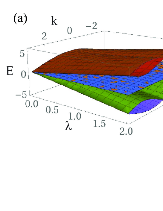
Figure 3: (a) The effect of the SOC with strength $\lambda$ on dispersion relations (10). (b) The dispersion relations explicitly shown for $\lambda=1$.

The two mutually symmetric SIGs, with $E>0$ and $E<0$, are located, respectively, above and beneath the DBs – namely, at

$$|E|>E_{\min}^{\mathrm{(SIG)}}\equiv 2\sqrt{1+\lambda^{2}+\sqrt{1+2\lambda^{2}}}.$$ (12)

Values $E_{\min}^{\mathrm{(SIG)}}$ correspond to maximum values of dispersion branches $E_{5,6}$ given by Eq. (10), which are attained at $k=\pm\arctan\left(\sqrt{2}\lambda\right)$.

Two analytical solutions for the CLSs inside the FBs of the linear system ($\gamma=\gamma_{1}=\zeta=0$) are

$$\mathbf{\Psi}_{n}^{(1)}= C\{\delta_{n,n_{0}}\left(\frac{\lambda^{2}-1}{2}(1+i),0,\frac{\lambda^{2}+1}{2}-i\frac{\lambda^{2}-1}{2},\lambda(1-i),0,i\lambda\right)$$

$$+\delta_{n+1,n_{0}}\left(\frac{\lambda^{2}-1}{2}-i\frac{\lambda^{2}+1}{2},0,\frac{\lambda^{2}+1}{2}(1+i),\lambda,0,0\right)\},$$

$$\mathbf{\Psi}_{n}^{(2)}= C\{\delta_{n,n_{0}}\left(\frac{\lambda^{2}-1}{2}-i\frac{\lambda^{2}+1}{2},0,-\frac{\lambda^{2}-1}{2}(1+i),-i\lambda,0,\lambda(1+i)\right)$$

$$+\delta_{n+1,n_{0}}\left(-\frac{\lambda^{2}+1}{2}(1+i),0,\frac{\lambda^{2}+1}{2}-i\frac{\lambda^{2}-1}{2},0,0,\lambda\right)\},$$ (13)

where $C$ is an arbitrary constant which determines the norm of the wave function, i.e., the number of atoms, in terms of the BEC model. Both solutions are CLSs with $U=2$, as they occupy two unit cells. In the limit of $\lambda\rightarrow 0$, they split into two obvious CLS states (7) set in adjacent cells. Thus, the SOC induces a change of the CLS class from $U=1$ at $\lambda=0$ to $U=2$ at $\lambda\neq 0$. The application of transformation (9) produces two additional symmetry-related solutions. The total norm of each of these solutions is given by $|\Psi|^{2}=2|C|^{2}(\lambda^{2}+1)^{2}$, as follows from Eq. (13).

Localized solutions are characterized by their participation number, which indicates the number of strongly excited sites:

$$P_{t}=\left(\sum_{n}|\Psi_{n}|^{2}\right)^{2}{\LARGE/}\sum_{n}|\Psi_{n}|^{4},\quad\mathbf{\Psi}_{n}\equiv\left\{a_{n}^{+},b_{n}^{+},c_{n}^{+},a_{n}^{-},b_{n}^{-},c_{n}^{-}\right\},$$ (14)

and by the spatial decay rate of the localized-mode’s tail vs. $n$.

For the linear-CLS solutions (13) obtained above, the participation number is

$$P_{t}=\frac{4(\lambda^{2}+1)^{4}}{(1/4)\left[(\lambda^{2}-1)^{4}+(\lambda^{2}+1)^{4}\right]+(1/2)(\lambda^{4}+1)^{2}+6\lambda^{4}}\;,$$ (15)

which yields the correct limit value $P_{t}(\lambda=0)=4$ in the limit of vanishing SOC. In the limit of strong SOC, it returns to the same limit value, $P_{t}(\lambda\rightarrow\infty)=4$ (practically, it is attained for $\lambda\geq 100$). At two values of the SOC strength, $\lambda=\sqrt{2\mp\sqrt{3}}\approx\left(0.52,1.93\right)$, expression (15) attains a maximum, $P_{t}=6$. At an intermediate point, $\lambda=1$, there is a local minimum, $P_{t}=16/3$.

The localized modes in the linear system are restricted to CLSs, sitting solely on the FBs, with $E=0$, see Eq. (10). In the absence of the SOC, there is no coupling between the equations for the two components, hence CLSs are generated in each component independently, the respective general solutions being linear superpositions of the simple stationary modes given by Eq. (7).

The SOC terms alter the shape of the CLS according to Eq. (13). In that case, the two components are coupled, and the structure of the compact modes changes. They feature complex field amplitudes, and, as said above, occupy (at least) two unit cells, see Fig. 4.

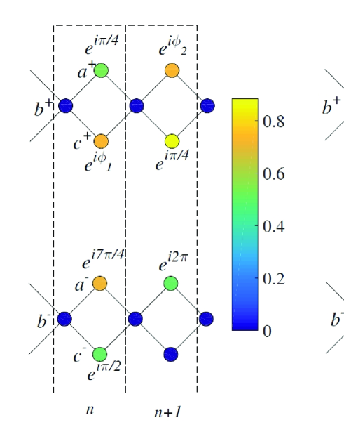
Figure 4: FB-CLS modes in the linear system, $\Psi_{n}^{(1)}$ (left) and $\Psi_{n}^{(2)}$ (right), as given by Eq. (13). Values of the phase, marked in the figure near the respective lattice sites, are $\phi_{1}=-\arctan\left(\lambda^{2}-\left(\lambda^{2}-1\right)/\left(\lambda^{2}+1\right)\right)$ and $\phi_{2}=-\arctan\left(\left(\lambda^{2}+1\right)/\left(\lambda^{2}-1\right)\right)$. The color code displays the squared absolute value of the wave function on each site and for each component. Note that the amplitudes strictly vanish on all $b$-sites. Here, $\lambda=2$.

IV Nonlinear localized modes

IV.1 Nonlinear CLSs and discrete solitons in the minigaps

The next, obviously important, objective is to explore the impact of nonlinearity in Eq. (8). We find that the CLSs survive solely if both the self- and cross-interactions are present, and the corresponding nonlinearity parameters are exactly equal, $\gamma=\gamma_{1}=\zeta$. This is clearly related to the above-mentioned validity condition for symmetry operation (9) in the nonlinear system. Being interested in self-trapped modes, we consider the case of attractive nonlinearity, with

$$\gamma=\gamma_{1}=\zeta>0.$$ (16)

For the opposite sign of the nonlinearity, essentially the same modes are obtained, with the opposite sign of the frequency, $E>0$.

The CLSs have precisely the same structure as given by Eq. (13) for the linear system, while the frequency of the nonlinear CLS families is

$$|E_{\mathrm{CLS}}|=\left(\gamma/2\right)|C|^{2}(\lambda^{2}+1)^{2}$$ (17)

[recall that $C$ is the amplitude of solution (13)]. Thus, the nonlinear CLS modes are found in the exact analytical form, although they exist solely under the strict condition (16). Equation (17) demonstrates that, varying $|C|^{2}$, one can tune the nonlinear CLS frequency to any positive value across the whole minigap, through the dispersive branches, and into the SIG. In particular, the existence of the CLSs in the spectral areas occupied by the dispersive bands implies that the CLSs may be identified as embedded solitons embedded , i.e., ones which are embedded into the bands of dispersive waves.

Straightforward algebraic manipulations show that, for the nonlinear CLS modes, which can be created only if $\zeta=\gamma=\gamma_{1}$, frequency $E$ and the total norm are related as

$$N=4|E|/\gamma.$$ (18)

This relationship does not depend on $\lambda$ and is not valid for discrete solitons (with exponentially decaying tails) considered below.

Both the linear stability analysis and direct simulations show that the nonlinear CLSs are stable for frequencies $E$ staying in a vicinity of the corresponding FB, viz., $|E|<E_{\mathrm{thr}}$. According to Eqs. (17) and (18), this implies that stable are CLSs with sufficiently small amplitudes and norms. The dependence of the stability threshold on the nonlinear-CLS frequency on $\lambda$ is shown in Fig. 5 in units of the minigap’s width, $W_{\mathrm{mg}}$ (11). In the limit of weak SOC, almost the whole minigap is populated by stable nonlinear CLSs (but note that the minigap itself becomes narrow in this case). On the contrary, the increase of the SOC strength $\lambda$ leads to a quick reduction of the relative stability threshold, which falls to $<0.01$ for $\lambda>1$.

To test the results of the linear-stability analysis, we simulated perturbed evolution of the nonlinear CLSs in the framework of Eq. (8). To this end, the nonlinear CLSs, belonging to the predicted stability and instability regions, with added a small amplitude random perturbation nashsoc , were used as initial conditions. In the course of the evolution, stable nonlinear CLSs keep constant phase differences between adjacent lattice sites, see Fig. 6. On the other hand, unstable CLSs feature irregular variations of the phase differences, which is accompanied by emission of energy into the lattice background. The latter feature is illustrated in Fig. 7 by plots for the participation ratio (14) of the respective modes.

In addition to the nonlinear CLSs which persist in the linear limit, the inclusion of the attractive nonlinearity gives rise to exponentially localized discrete solitons (DSs), which are similar to usual DSs in nonlinear lattices discrete , see examples in Figs. 8 and 9. The structure of the DS tails, and the comparison to the CLS shape [taken from Fig. 8(d)], are shown on the logarithmic scale in Fig. 10. A drastic difference of the discrete solitons from the CLSs is that the DSs exist as well when the cross-interaction coefficient, $\zeta$, is different from its self-interaction counterparts, $\gamma$ and $\gamma_{1}$ (for instance, in Fig. 8 $\gamma=\gamma_{1}=1$ but $\zeta=0$).

Different DS modes are numerically obtained by changing the respective input, i.e., its shape and norm, and ratios between the self- and cross-interaction parameters, $\gamma$, $\gamma_{1}$, and $\zeta$. Similar to the CLSs, the DSs have narrow stability regions inside the minigaps. Exact location of boundaries of the regions is a challenging issue, as they are sensitive to variations of all the parameters. On the other hand, the existence and stability of similar exponentially localized DSs in minigaps was studied in other lattice models (see, e.g., Ref. chaosmi . Therefore, we here focus on accurate delineation of the stability area for the CLSs in the minigaps of the nonlinear lattice, which is a new problem.

The simulations demonstrate that perturbed stable states give rise to robust breathers periodically oscillating in time. Outside of the narrow stability regions found in the neighborhood of the FB, unstable perturbed CLSs and DSs spread over the entire lattice in the course of simulations. The evolution of participation number for perturbed stable and unstable DSs of type shown in Fig. 8 (d) is displayed in Fig. 7, confirming the predictions of the linear-stability analysis. The spreading rate of unstable DSs is indeed determined by unstable EVs for these modes.

Figure 5: The linear stability diagram for nonlinear CLSs. Stable CLSs exist for $E<E_{\mathrm{thr}}$, which is plotted, in the log scale, in units of the minigap width $W_{\mathrm{mg}}$ [see Eq. (11)]. Nonlinearity parameters are $\gamma=\gamma_{1}=\zeta=1$.

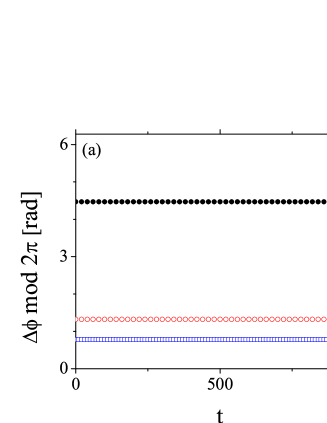
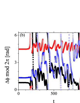
Figure 6: (a) The phase difference between the field components of the stable (slightly perturbed) CLSs at adjacent sites: $a_{n+1}^{+}$ and $a_{n}^{+}$ (black circles), $c_{n+1}^{+}$ and $c_{n}^{+}$ (red empty circles), $a_{n+1}^{-}$ and $a_{n}^{-}$ (blue squares), vs. time. (b) The same for an unstable nonlinear CLSs. The SOC strength is $\lambda=2$. The stable and unstable CLSs have, respectively, $E=-0.0009,\,N=0.0036$, and $E=-1.901,\,N=0.06$. The nonlinearity parameters are $\gamma=\gamma_{1}=\zeta=1$.

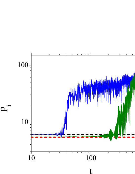
Figure 7: The participation number of a stable nonlinear CLS, with $E=-0.0009,\,N=0.0036$ (the black dashed line) and of an unstable one, with $E=-1.901,\,N=0.06$ (the blue solid line) versus time. Nonlinearity parameters are $\gamma=\gamma_{1}=\zeta=1$. Also shown are the time dependence of the participation ratio for a stable ($E=-0.01,\,N=0.0036$, the red dashed line) and unstable ($E=-0.49,\,N=0.27$, the green solid line) discrete solitons (DSs). The SOC strength is $\lambda=2$.

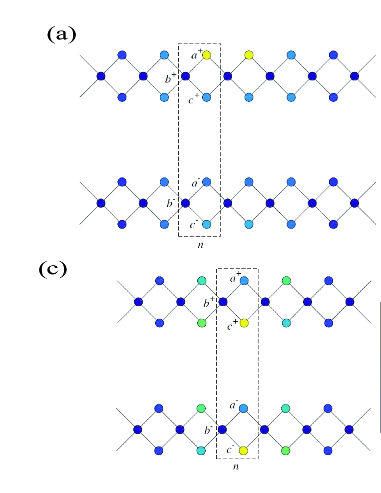
Figure 8: Different discrete-soliton modes for $\gamma=\gamma_{1}=1,\,\zeta=0$ and $\lambda=2$.

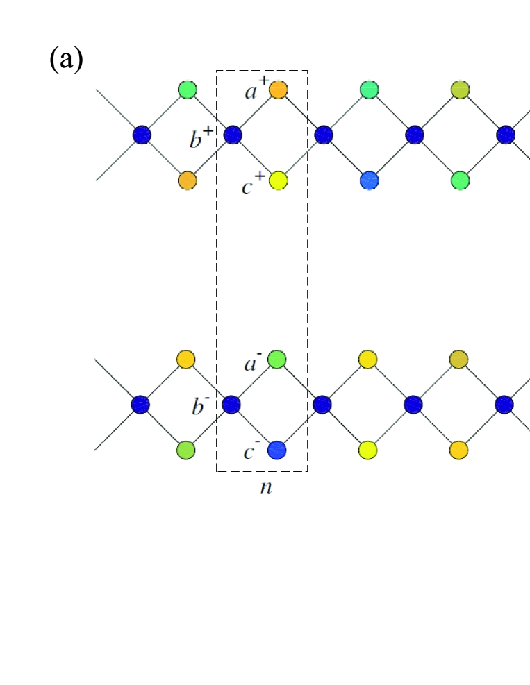
Figure 9: Different discrete-soliton modes for $\gamma=\gamma_{1}=\,\zeta=1$ and $\lambda=2$.

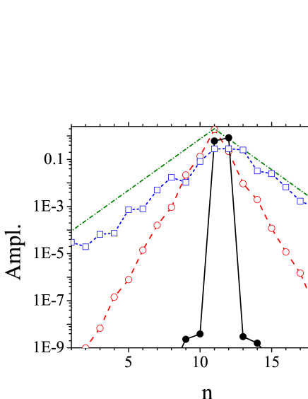
Figure 10: The spatial structure of normalized tails of different discrete solitons on the log-log scale: a CLS (the black line with circles), the discrete soliton, shown in Fig. 8(d) (the blue dashed line with empty squares), and the discrete soliton found in the semi-infinite gap (the red line with empty circles). For comparison, the line with constant slope $-1$ is shown as the olive dot-dashed one. Parameters are $\lambda=2$, $\gamma_{1}=\gamma=\zeta=1$ for the modes denoted by solid lines, and $\lambda=2$, $\gamma_{1}=\gamma=1$, $\zeta=0$ for those denoted by dashed lines. The values of $E$ and $N$ are the same as in Fig. 7.

Finally, it has been checked that stable CLSs and DSs may coexist in a vicinity of the FB. They all are characterized by mutually close (and small) values of the norm. In fact, their shapes are close too, apart from the presence of the exponentially decaying tails in the DSs, which are absent in the CLSs. The DS solutions’ existence area covers the entire minigaps, but their stability region is a narrow strip adjacent to the FB. Unlike the CLSs, DS states do not exists at values of $E$ belonging to the DBs, i.e., the DSs cannot be modes of the embedded type.

IV.2 Localized modes in the semi-infinite gap (SIG)

It is natural to explore the existence and stability of localized states in the SIG. First, as mentioned above, the CLSs can be found in the SIG. Note that the simple relation between the CLS norm and frequency, given by Eq. (18), applies to the SIG as well. The stability area of the CLSs inside of SIG has been identified too, through the linear-stability analysis and direct simulations alike. The stability area in the plane of $\left(E,\lambda\right)$ is shown in Fig. 11, cf. the stability region for the CLSs in the minigaps, shown in Fig. 5. Similar to the fact that the CLSs are stable only a small part of the minigap, the stability area occupies only a small portion of the SIG.

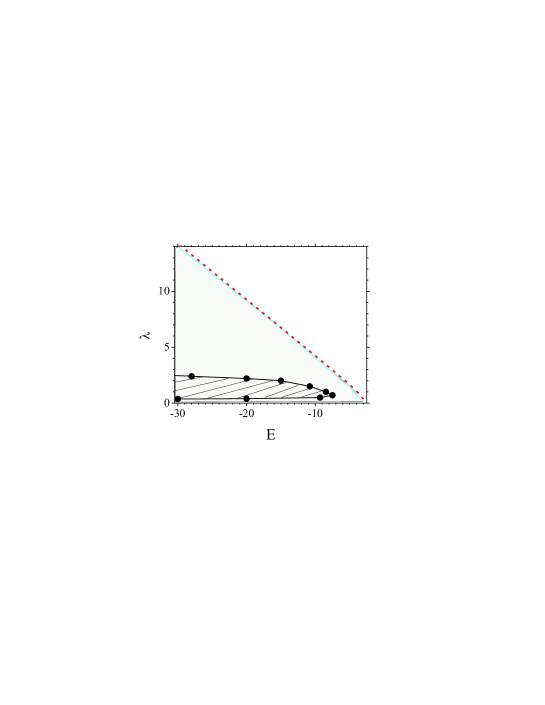
Figure 11: The CLSs and one-peak DS found inside the SIG are stable in the shaded and the gray area below the blue curve, respectively, in the plane of $\left(E\text{,}\lambda\right)$. The nonlinearity parameters are fixed as $\gamma=\gamma_{1}=\zeta=1$ for both solution types (recall that the CLS does not exist if the these coefficients are not equal). The dashed line shows the SIG boundary, as given by the inversion of Eq. (12): $\lambda=\sqrt{E^{2}/4+E/\sqrt{2}}$.

In the absence of the SOC ($\lambda=0$), DSs, which are characterized by the largest amplitude at site $b$ (on the contrary to the CLSs, which have zero amplitudes at $b$), also exist inside the SIG. They are found to be stable at $E<-5$ for $\gamma,\,\gamma_{1}>0$ (or at $E>5$ for $\gamma,\,\gamma_{1}<0$). A typical example of such a mode is displayed in Fig. 12(a).

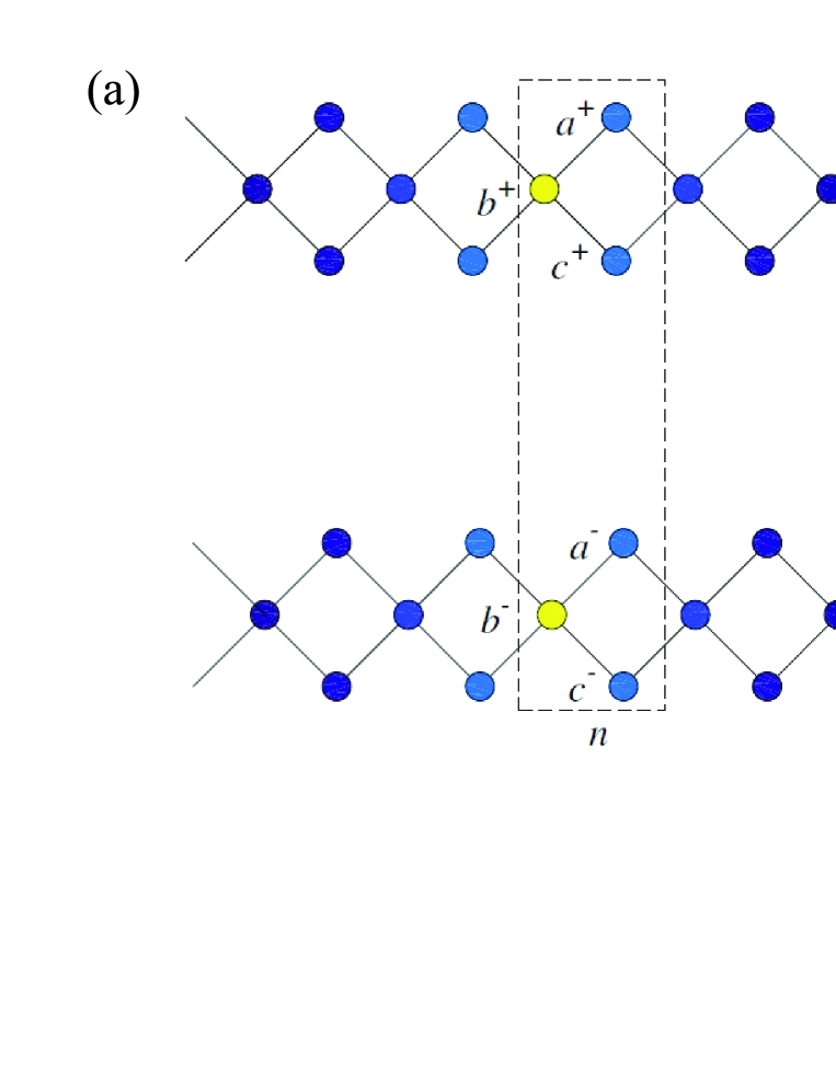
Figure 12: Examples of stable DS mode found in the SIG, for parameters (a) $\lambda=0$, $E=-4.99,\,N=5.03$, and (b) $\lambda=1$, $E=-9.99,\,N=9.79$.

In the presence of the SOC, single-peak DSs are found in the SIG too. Their symmetry with respect to the central $(b)$ site is broken by the SOC. The stability region of the single-peak DSs almost overlaps with the SIG area, as shown in Fig. 11 (the gray area bounded by the blue solid curve). An example of the stable DS is shown for $\lambda=2$, $\gamma=\gamma_{1}=\zeta=1$ in Fig. 12(b). The affinity of these states to the usual discrete solitons is confirmed by plotting tails of the corresponding solutions in Fig. 10 (the red line with empty circles). For the sake of comparison, an exponentially decaying function is shown by the green line in the same plot.

V Conclusions

We have introduced a dynamical lattice system, which may be realized for the two-component BEC with the SOC (spin-orbit coupling), loaded into the optically imprinted ribbon with the structure of the diamond chain, that serves as a paradigm for realizing FB (flatband) spectra. The system includes interactions between its components, both nonlinear and linear, the latter mediated by the SOC. The linear version of the system, in the absence of the SOC, is characterized by the spectrum which consists of a pair of DBs (dispersive bands) which touch the FB at the edge of the corresponding Brillouin zone, for each component. Such a linear decoupled system creates CLS (compact localized states) in each component which extend over one unit cell and belong to the class $U=1$, at a single value of the frequency which exactly corresponds to the FB. The introduction of the SOC changes the spectrum, keeping the double-degenerate FBs and opening narrow minigaps between them and the DBs. The CLSs remain available in the exact analytical form. They increase their size to $U=2$, and can be viewed as a bound state of two CLSs of class $U=1$, with an appropriate phase and amplitude modulation, depending on the strength of SOC. In the presence of the onsite self-attractive cubic nonlinearity, we have shown that the CLSs persist in the form of exact analytical solutions. Their frequency can be tuned throughout the minigap, as well as into the SIG (semi-infinite gap). Parallel to that, usual DSs (discrete solitons) with exponentially decaying tails have been found too, in a numerical form, in the minigap and SIG alike. Both the CLS and DS modes are stable inside of the minigap in narrow stripes abutting on the FB. Stability areas for the CLS and DS families have been found in the SIG too, also being small in comparison with the SIG size.

A main motivation for the interest in CLSs and FBs is due to the macroscopic degeneracy they enforce. Such macroscopic degeneracies are usually removed due to external perturbations, leading to new eigenstates, whose properties are sensitively depending on the type of perturbation added. In this work we show that spin-orbit coupling with cold atoms in optical lattices acts as a degeneracy-preserving perturbation. We also find that properly tuned interactions destroy the notion of a band structure, yet preserve the CLSs which simply detune their frequencies. A detuning of these interactions will finally destroy the CLSs.

In addition to that, in this work we have demonstrated that the presence of the FB strongly affects not only the CLSs but also regular DSs. It is expected that these DSs will keep their properties even if a perturbation of the system will lend the FB a weak curvature.

As a development of the analysis, it may be interesting to analyze a fully two-dimensional version of the system. In particular, modes in the form of stable localized vortices have not been found in the present system, both with and without the SOC terms. It is plausible that vortex modes may exist in the fully two-dimensional lattice.

References

- (1) O. Derzhko, J. Richter and M. Maksymenko, Int. J. Mod. Phys. B 29 1530007 (2015).
- (2) D. Guzman-Silva, C. Mejia-Cortes, M. A. Bandres, M. C. Rechtsman, S. Weimann, S. Nolte, M. Segev, A. Szameit, and R. A. Vicencio, New. J. Phys. 16, 063061 (2014).
- (3) N. Masumoto, N. Y. Kim, T. Burnes, K. Kusudo, A. Löffer, S. Höfling, A. Forchel, and Y. Yamamoto, New. J. Phys. 14, 065002 (2012).
- (4) S. Taie, H. Ozawa, T. Ichinose, T. Nishio, S. Nakajima, and Y. Takahashi, Science Advances 1, e1500854 (2015).
- (5) S. Flach, D. Leykam, J. D. Bodyfelt, P. Matthies, and A. S. Desyatnikov, EPL 105, 30001 (2014).
- (6) A. E. Miroshnichenko, S. Flach and Y. S. Kivshar, Rev. Mod. Phys. 82, 2257 (2010).
- (7) R. A. Vicencio, C. Cantillano, L. Morales-Inostroza, B. Real, C. Mejia-Cortes, S. Weimann, A. Szameit, and M. I. Molina, Phys. Rev. Lett. 114, 245503 (2015).
- (8) S. Mukherjee, A. Spracklen, D. Choudhury, N. Goldman, P. Öhberg, E. Andersson, and R. R. Thomson, Phys. Rev. Lett. 114, 245504 (2015).
- (9) S Weimann, L. Morales-Inostroza, B. Real, C. Cantillano, A. Szameit and R. A. Vicencio, Optics Letters 41, 2414 (2016)
- (10) F. Baboux, L. Ge, T. Jacqmin, M. Biondi, E. Galopin, A. Lemaître, L. Le Gratiet, I. Sagnes, S. Schmidt, H. E. Türeci, A. Amo, and J. Bloch, Phys. Rev. Lett. 116, 066402 (2016).
- (11) Daniel Leykam, Joshua D. Bodyfelt, Anton S. Desyatnikov and S. Flach, arXiv:1601.03784 (2016).
- (12) J. D. Bodyfelt, D. Leykam, C. Danieli, X. Yu and S. Flach, Phys. Rev. Lett. 113 236403 (2014).
- (13) Carlo Danieli, Joshua D. Bodyfelt and S. Flach, Phys. Rev. B 91 235134 (2015).
- (14) R. Khomeriki and S. Flach, Phys. Rev. Lett. 116, 245301 (2016).
- (15) R. A. Vicencio and M. Johansson, Phys. Rev. A 87, 061803(R) (2013).
- (16) D. Leykam, S. Flach, O. Bahat-Treidel, and A. S. Desyatnikov, Phys. Rev. B, 88, 224203 (2013);
- (17) M. Johannson, U. Naether, and R. A. Vicencio, Phys. Rev. E 92, 032912 (2015).
- (18) D. Lopez-Gonzalez and M. I. Molina, Phys. Rev. A 93, 043847 (2016).
- (19) D. L. Campbell, G. Juzeliūnas, and I. B. Spielman, Phys. Rev. A 84, 025602 (2011); Y. J. Lin, K. Jimenez-Garcia, and I. B. Spielman, Nature 471, 83 (2011); V. Galitski I. B. and Spielman, Nature 494, 49 (2013); H. Zhai, Rep. Prog. Phys. 78, 026001 (2015).
- (20) H. Sakaguchi and B. Malomed, Phys. Rev. E 90, 062922 (2014).
- (21) P. P. Beličev, G. Gligorić, J. Petrović, A. Maluckov, Lj. Hadžievski, and B. A. Malomed, Journal of Physics B: Atomic, Molecular and Optical Physics 48, 065301 (2015).
- (22) G. Gligorić, A. Maluckov, Lj. Hadžievski, and B. A. Malomed, Phys. Rev. A 78, 063615 (2008).
- (23) K. Yagasaki, A. R. Champneys, and B. A. Malomed, Nonlinearity 18, 2591 (2005).
- (24) F. Lederer, G. I. Stegeman, D. N. Christodoulides, G. Assanto, M. Segev, and Y. Silberberg, Phys. Rep. 463, 1 (2008).
- (25) G. Gligoric, A. Maluckov, L. Hadzievski, and B. A. Malomed, Chaos 24, 023124 (2014).