Matter-wave dark solitons in box-like traps

Abstract

Motivated by the experimental development of quasi-homogeneous Bose-Einstein condensates confined in box-like traps, we study numerically the dynamics of dark solitons in such traps at zero temperature. We consider the cases where the side walls of the box potential rise either as a power-law or a Gaussian. While the soliton propagates through the homogeneous interior of the box without dissipation, it typically dissipates energy during a reflection from a wall through the emission of sound waves, causing a slight increase in the soliton’s speed. We characterise this energy loss as a function of the wall parameters. Moreover, over multiple oscillations and reflections in the box-like trap, the energy loss and speed increase of the soliton can be significant, although the decay eventually becomes stabilized when the soliton equilibrates with the ambient sound field.

I Introduction

Dark solitons are one-dimensional non-dispersive waves which arise in defocussing nonlinear systems as localized depletions of the field envelope Kivshar1998 . To date, they have been observed in systems ranging from optical fibres Emplit ; Krokel ; Weiner , magnetic films Chen , plasmas Heidemann , waveguide arrays Smirnov , to water Chabchoub and atomic Bose-Einstein condensates Frantzeskakis2010 . This work is concerned with the last system; here the matter field of the gas experiences a defocussing cubic nonlinearity arising from the repulsive short-range atomic interactions. In the limit of zero temperature, the mean matter field is governed by a cubic nonlinear Schrd̈inger equation (NLSE) called the Gross-Pitaevskii equation (GPE) Stenholm-PR363-2002heuristic ; Carretero-N21-2008nonlinear ; Gross-NC20-1961structure ; Gross-1963 ; Pitaevskii-1961 . Many experiments have generated and probed these matter-wave dark solitons Burger1999 ; Denschlag2000 ; Dutton2001 ; Engels2007 ; Jo2007 ; Becker2008 ; Chang2008 ; Stellmer2008 ; Weller2008 ; Aycock2016 .

A necessary feature of an atomic condensate is the trapping potential required to confine it in space. When the trapping potential is highly elongated in one direction compared to the other two, the condensate becomes effectively one-dimensional, and its longitudinal dynamics is described by the 1D GPE. If the system is homogeneous in the longitudinal direction, the GPE is integrable and supports exact dark soliton solutions. Dark solitons appear as a local notch in the atomic density with a phase slip across it, and travel with constant speed Reinhardt1997 ; Frantzeskakis2010 while retaining their shape. However, the presence of confinement in the longitudinal direction breaks the “complete integrability” of the governing equation and causes the dark soliton to decay via the emission of sound waves Busch2000 ; Huang2002 ; Parker2003 ; Pelinovsky2005 ; Parker2010 . An analogous effect arises in nonlinear optics due to inhomogeneities of the optical nonlinearity Kivshar1998 ; Pelinovsky1996 . In condensates, dark solitons may also decay through thermal dissipation Fedichev1999 ; Muryshev2002 ; Jackson2007 and transverse ‘snaking’ instability into vortex pairs or rings Muryshev1999 ; Carr2000 ; Feder2000 ; Anderson2001 ; Dutton2001 ; Theocharis2007 ; Hoefer2016 ; both decay channels can be effectively eliminated by operating at ultracold temperatures and in tight 1D geometries, respectively.

To date, the trapping potentials most commonly used have been harmonic (quadratic in the distance from the centre of the condensate). Evolution and stability of dark solitons moving under a longitudinal harmonic potential have been carefully analyzed. We know that the soliton tends to oscillate back and forth through the condensate at a fixed proportion of the trap’s frequency Fedichev1999 ; Muryshev1999 ; Busch2000 ; Huang2002 ; Theocharis2007 . While the inhomogeneous potential leads to sound emission from the soliton, the harmonic trap uniquely supports an equilibrium between sound emission and reabsorption, such that the soliton decay is stabilized Parker2003 ; Parker2010 . Theoretical work has also considered the radiative behaviour of a dark soliton moving under the effect of linear potentials and steps Parker2003b , perturbed harmonic traps Busch2000 ; Parker2003 ; Allen2011 , optical lattices Kevrekidis2003 ; Parker2004 , localized obstacles Frantzeskakis2002 ; Parker2003b ; Radouani2003 ; Radouani2004 ; Proukakis2004 ; Bilas2005a ; Hans2015 , anharmonic traps Radouani2003 ; Parker2010 and disordered potentials Bilas2005b . For slowly-varying potentials, it is found that the power emitted by the solition is proportional to the square of the soliton’s acceleration Kivshar1998 ; Pelinovsky1996 ; Parker2003 .

Increasingly, however, experiments are employing box-like traps to produce quasi-homogeneous condensates. Such traps have been realized in one Meyrath ; VanEs , two Chomaz and three Gaunt dimensions (with tight harmonic trapping in the remaining directions in the 1D and 2D cases). These new traps feature flat-bottomed central regions and end-cap potential provided by optical or electromagnetic fields; the boundaries are therefore soft, unlike infinite hard walls of existing mathematical models. For example, the 1D optical box trap of Ref. Meyrath featured approximately Gaussian walls, while the 2D and 3D optical box traps of Refs. Gaunt ; Chomaz had a power-law scaling in the range from $x^{10}$ to $x^{15}$. In the bulk of the box-trap, where the density is homogeneous, a dark soliton is expected to propagate at constant speed and retain its shape; however, the nature of the reflection of the soliton from boundaries which are steeper than the traditional quadratic dependence and softer than hard boundaries is still unexplored. Here we seek to address this problem through a systematic computational study of the reflection of a dark soliton from power-law and Gaussian walls.

II Mathematical model

We consider an atomic condensate in the limit of zero-temperature, with arbitrary trapping $V(x)$ along the axis and tight harmonic trapping in the transverse directions. Assuming the quasi-1D configuration, the condensate is described by the one-dimensional wavefunction, $\Psi(x,t)$; the atomic density follows as $n(x,t)=|\Psi(x,t)|^{2}$. The dynamical evolution equation of $\Psi$ is governed by the one-dimensional Gross-Pitaevskii equation,

$$i\hbar\Psi_{t}=-\frac{\hbar^{2}}{2m}\Psi_{xx}+V(x)\Psi+g|\Psi|^{2}\Psi,$$ (II.1)

where $m$ is the atomic mass and the nonlinear coefficient $g=4\pi\hbar^{2}a_{s}/m$ arises from short-range atomic interactions of s-wave scattering length $a_{s}$, and subscripts denote partial derivatives.

Since we are concerned with quasi-homogeneous condensates, it is natural to adopt units relating to the bulk of the 1D condensate, where the density is $n_{0}=\sqrt{\mu_{0}/g}$ Primer , and the chemical potential $\mu_{0}$ is the characteristic energy scale. The healing length $\xi_{0}=\hbar/\sqrt{mn_{0}g}$ is the minimum spatial scale of density variations, and the speed of sound $c=\sqrt{n_{0}g/m}$ is the typical speed scale; the natural timescale of the bulk condensate follows as $\xi_{0}/c_{0}$. Employing these quantities as units leads to the following dimensionless GPE Primer ,

$${\textrm{i}}u_{t}=-\frac{1}{2}u_{xx}+|u|^{2}u+V(x)u,$$ (II.2)

where all variables are in their dimensionless form. Throughout the rest of this paper we employ dimensionless variables.

The total energy of the condensate, given by the integral,

$$E_{\rm tot}=\int\left(\frac{1}{2}\left|\psi_{x}\right|^{2}+V(x)|\psi|^{2}+\frac{1}{2}|\psi|^{4}\right)~{}{\rm d}x$$ (II.3)

is conserved within the GPE, as confirmed by our numerical simulations.

Equation (II.2) have been investigated over the years in terms of the “complete integrability” (see BruguarinoJMP51-2010 and reference therein). This property (even though still not univocally defined) regards the existence of infinite number of conservation laws and the possibility of relating the nonlinear PDE (partial differential equation) to a linear PDE by an explicit transformation. The main feature is that Eq. (II.2) is not completely integrable except for the case $V(x)=ax+b$, with $a$ and $b$ constants BruguarinoJMP51-2010 . For $V(x)=0$, the GP equation (II.2) has the following exact dark soliton solution Kivshar1998 ; Frantzeskakis2010 ,

$$u=\left\{k\tanh\left[k\left(x-tv-s_{0}\right)\right]+{\textrm{i}}v\right\}e^{-{\textrm{i}}\left(t-\theta_{0}\right)},$$ (II.4)

where $k=\sqrt{1-v^{2}}$ is the amplitude of the dark soliton, $v$ is the soliton’s speed (and $|v|<1$) and $s_{0}$ and $\theta_{0}$ are arbitrary reference values of the position and phase of the soliton. The normalized dark soliton’s energy is Kivshar1998 ,

$$E_{\rm sol}=\frac{4}{3}(1-v^{2})^{3/2}.$$ (II.5)

In the absence of the external potential ($V(x)=0$), the soliton (II.4) propagates without any loss along the BEC. This lossless motion results from the perfect balance of nonlinear ($|u|^{2}u$) and linear ($u_{xx}$) terms in Eq. (II.2). In optics the soliton is the envelope of different plane waves of different frequencies and phase velocities which moves with the group speed $v$, and the two terms induce self-phase modulation (SPM) and group velocity dispersion (GVD), respectively. When the balance between the two terms ceases or is altered, some harmonic components acquire more energy or new harmonics are generated by the nonlinearity, and what one sees is the generation of small-amplitude density (sound) waves (as also explained in Section IV).

Our work is based on numerical simulations of the dimensionless 1D GPE (II.2). Numerical time integration of the equation is performed using the split-step Fourier method. The initial condition consists of the ground state condensate solution obtained via the technique of imaginary-time propagation of the GPE, into which a dark soliton solution of (II.4) is multiplied at the origin (this solution is appropriate because at the origin the system is locally homogeneous). During the course of the longest simulations (e.g. Fig. 6) the total energy of the system, $E_{\rm tot}$, changes by less than 1 part in $10^{4}$.

We consider two types of quasi-homogeneous box potentials. The first, termed the power-law box and motivated by the experiments of Refs. Gaunt ; Chomaz , is characterised by boundaries where the potential increases as a power of the spatial coordinate. The overall potential has the form,

$$V(x)=\left\{\begin{array}[]{ll}0&\mbox{ if $|x|\leq w$}\\ \left(\frac{|x|-w}{l}\right)^{\alpha}&\mbox{ if $w<|x|\leq L$}\end{array}\right.$$ (II.6)

where $\alpha$ is the exponent of the potential at the boundaries, $2w$ is the width of the flat part of the potential, and $2L$ is the whole width of the potential. This potential is shown schematically in Fig. 1(a). The width of the boundary is then $\displaystyle L-w$. The height of the potential wall is given by $\displaystyle V_{0}=V(L)=\left(\frac{L-w}{l}\right)^{\alpha}$, and $l$ is a parameter used to enstablish the height of the side of the potential. The parameters we modify in our numerical experiments are the exponent $\alpha$, the height of the boundary potential $V_{0}$ and the width of the boundary potential $\displaystyle L-w$.

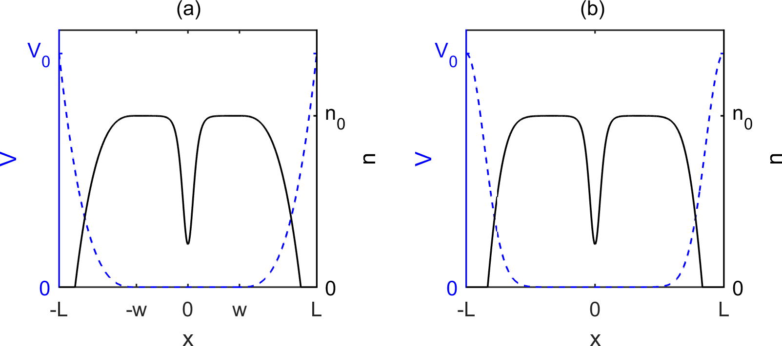
Figure 1: (Color online) Schematic representations of the potential $V(x)$ and density $n(x)$ in our box traps, with a dark soliton at the origin. (a) In the power-law box, the potential is flat ($V=0$) over the region $[-w,w]$, and increases as a power-law outside this region, reaching the maximum value $V_{0}=V(L)$ at the edges $x=\pm L$ of the box. (b) In the exponential box, Gaussian potentials (centred at $x=\pm L$ and with width $L-w$ form the end-caps of the box.

The second form of quasi-homogeneous box trap is that where the end-caps are formed by laser-induced Gaussian potentials, as used in Refs. Meyrath . This box, termed the exponential box and shown schematically in Fig. 1(b), has the form,

$$V(x)=V_{0}\left[{\rm e}^{-\frac{\left(x-L\right)^{2}}{c^{2}}}+{\rm e}^{-\frac{\left(x+L\right)^{2}}{c^{2}}}\right].$$ (II.7)

The crest of the Gaussian potentials are located at $x=\pm L$, $V_{0}$ is their amplitude, and $c$ characterises their width. As in the power-law box, we perform numerical experiments to explore the dependence on the amplitude $V_{0}$ and the width $c$ of the boundary potentials on the soliton’s motion.

III Results

In Section III.1 we shall examine a single reflection of a dark soliton with a boundary of the box, for both the power-law and exponential box types. Later, in Section III.2, we shall extend our analysis to multiple oscillations and reflections in the box. Throughout this section we set the box width to the arbitrary value $L=80$.

III.1 Single reflection

A dark soliton (II.4) is introduced at the origin with arbitrary speed $v=0.5$ (in the positive $x$ direction) and launched at the $x=L$ boundary of the power-law box. Figure 2 shows the dynamics during the reflection from a power-law boundary with fixed width $w=60$ and amplitude $V_{0}=30$, and three different exponents. For $\alpha=0.5$ (a, b), the soliton reflects elastically. Here the boundary looks effectively like a hard wall - up to the typical energy scale of the condensate, $V\sim 1$, the potential remains very steep. For a quadratic potential $\alpha=2$ (c, d), however, a pulse of sound waves is generated during the reflection which propagate in the negative $x$ direction at the speed of sound. These waves have amplitude of around $\sim 5\%$ of the peak density. For a much higher exponent $\alpha=13$ (e, f), again sound waves are emitted during the reflection, with a slightly reduced amplitude.

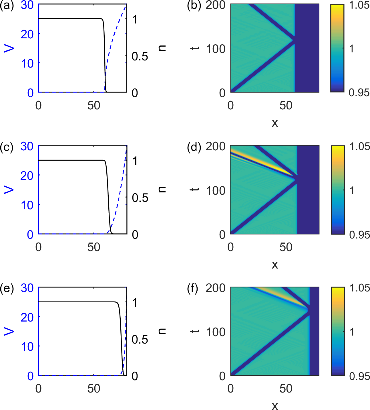
Figure 2: (Color online). Examples of the reflection of a $v=0.5$ dark soliton from the boundary of a power-law box. Shown is (a, c, e) the box potential (II.6) and ground-state density profile, and (b, d, f) the evolution of the density during the reflection. Plots (a, b) correspond to a power-law exponent of $\alpha=0.5$, (c, d) correspond to $\alpha=2$ and (e, f) correspond to $\alpha=13$. The remaining parameters are fixed to $L=80$, $w=60$ and $V_{0}=30$.

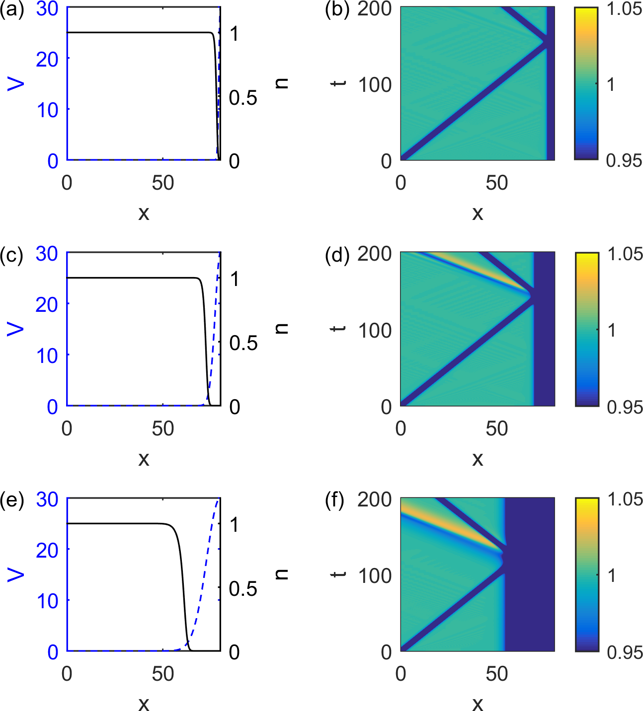
Figure 3: (Color online). Examples of the reflection of a $v=0.5$ dark soliton from the boundary of an exponential box. Shown is (a, c, e) the box potential (II.6) and ground-state density profile, and (b, d, f) the evolution of the density during the reflection. Plots (a, b) correspond to a Gaussian width of $c=1$, (c, d) correspond to $c=4$ and (e, f) correspond to $c=10$. The remaining parameters are fixed to $L=80$ and $V_{0}=30$.

Figure 3 shows example dynamics for the soliton reflecting from an exponential boundary. Here the amplitude of the boundaries is fixed to $V(L)=30$ and the width $c$ varied. For a narrow edge $c=1$ (a, b) the soliton reflects elastically. Like above, the boundary appears as a hard wall. However, for wider boundaries, $c=4$ (c, d) and $c=10$ (e, f), the soliton dissipates energy through the emission of sound waves.

It is evident that the reflection of the dark soliton from the soft boundary is typically dissipative (where we are referring to the dissipation of the soliton; the total energy of the system is conserved), although the amount of sound radiated is sensitive to the boundary parameters. Now we characterise this dissipation in terms of the energy lost from the soliton. The soliton’s energy $E_{\rm sol}$ is evaluated numerically before and after the reflection. This is performed by calculating the energy associated with the soliton within a small region around the soliton, according to the scheme described in Ref. Parker2010 . We report the proportional loss in soliton energy after the reflection, normalized with respect to its initial value, and denote this as $\Delta E_{\rm sol}$.

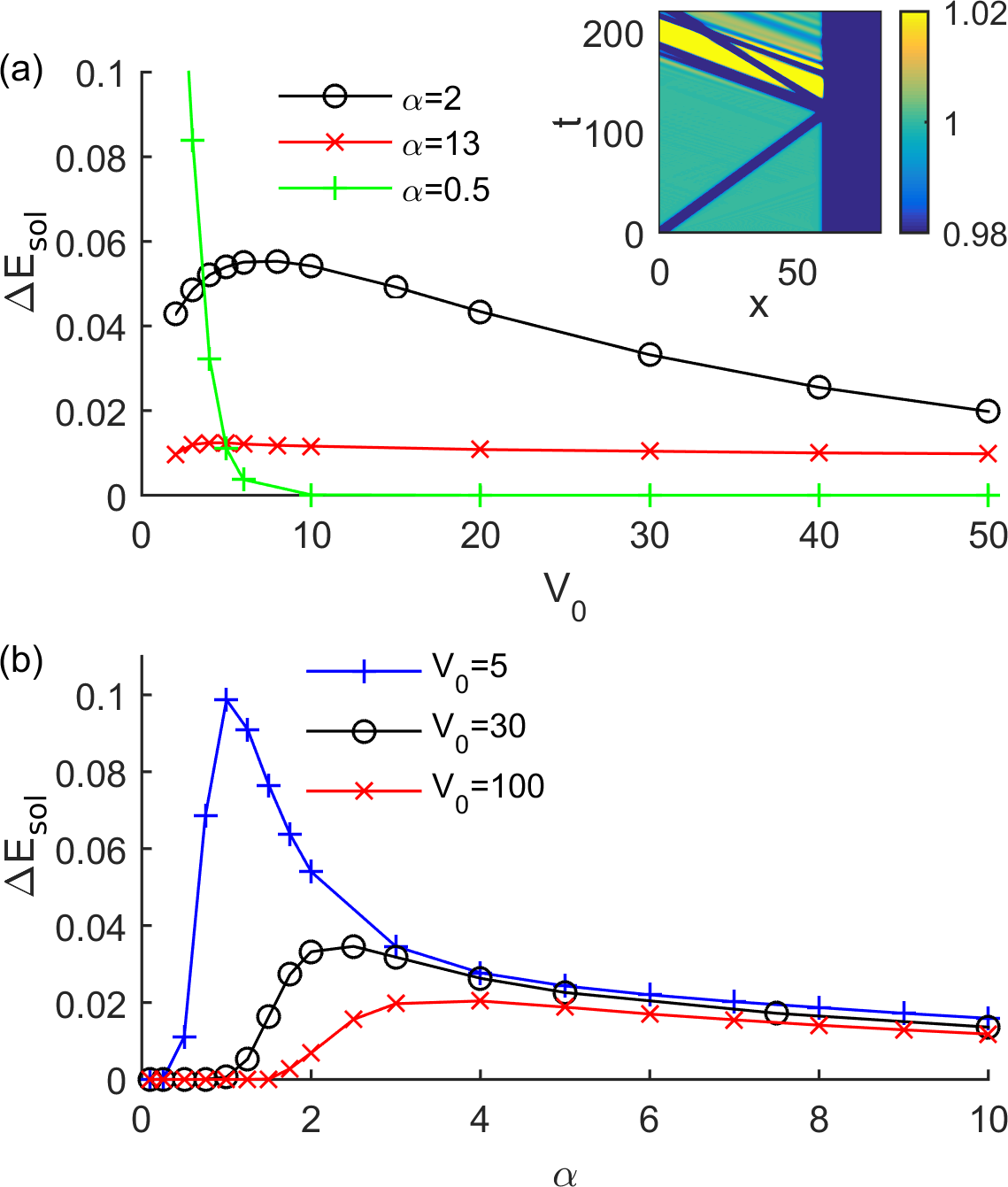
Figure 4: (Color online). Energy loss in the dark soliton (normalized by its initial energy) $\Delta E_{\rm sol}$ due to a reflection against a power-law boundary. Panel (a) shows this energy loss as a function of the amplitude of the boundary potential $V(L)$, for three values of the exponent $\alpha$. Panel (b) shows $\Delta E_{\rm sol}$ as a function of the exponent $\alpha$ for fixed potential amplitude $V_{0}$. In (a) the inset is for $\alpha=0.5$ and $V_{0}=2$, showing anomalously high sound emission.

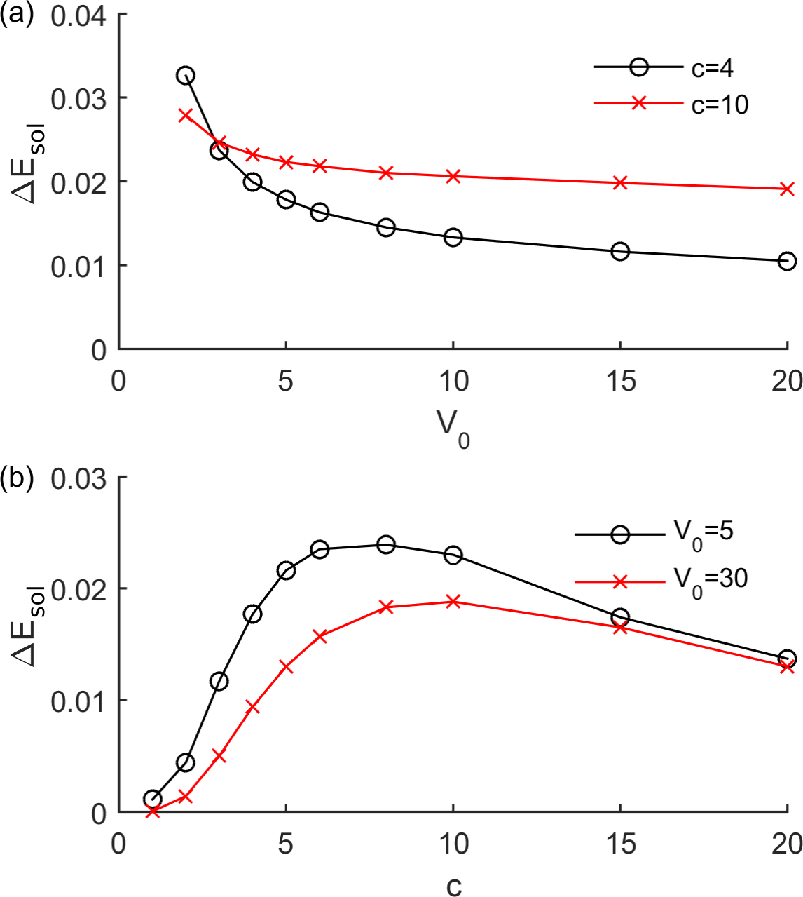
Figure 5: (Color online). Energy loss in the dark soliton (normalized by its initial energy) $\Delta E_{\rm sol}$ due to a reflection against an exponential boundary. Panel (a) shows this energy loss as a function of the amplitude of the boundary potential $V_{0}$, for two values of the Gaussian width $c$, while (b) displays it as a function of the $c$ for fixed potential amplitude $V_{0}$.

Figure 4(a) shows the energy loss for the power-law trap as a function of the amplitude of the boundary potential $V_{0}$, for three values of the potential exponent $\alpha$. Note that we limit our analysis to $V_{0}\geq 2$; below this range the potential does not fully confine the condensate. For $\alpha=2$ and $\alpha=13$, the energy loss increases to a maximum at moderate $V_{0}$ ($V_{0}\sim 5-10$ for these cases), before decaying with increasinging $V_{0}$. This is typical of the general behaviour for $\alpha\geq 1$. It is worth noting that the softer boundary, $\alpha=2$, gives the most energy loss (up to $5\%$), and that the energy loss decays very slowly with $V_{0}$, and so causes significant dissipation even for large amplitudes. For $\alpha<1$, however, the trend is distinct. For large $V_{0}$, sound emission is heavily suppressed; this is because for $\alpha<1$ the boundary potential rises up with a very large gradient (which decreases with distance into the boundary). As such, for $V_{0}\gg 1$ the condensate/soliton effectively experiences a hard wall potential. For smaller $V_{0}$, however, the condensate/soliton experiences the low gradient region of the boundary, inducing sound emission. The energy loss increases rapidly as $V_{0}$ is decreased towards the value of $2$, enchanced by an unusual effect where sound waves are generated from the boundary even after the soliton has left the boundary (see inset of Fig. 4(b)).

Figure 4(b) shows the energy loss as a function of the exponent $\alpha$, for three values of the potential amplitude. The general behaviour is that the energy loss is typically vanishingly small for small $\alpha$, due to the hard-wall effect mentioned above, and is also small for very large $\alpha$, since the potential increases rapidly and also begins to approximate a hard wall. However, in between these limits, the energy loss reaches maximum; this position of this maximum is dependent on $\alpha$ but typically lies in the range $1<\alpha<5$.

Similarly, we have explored the energy loss from a single reflection of an exponential boundary. For fixed width $c$ (Fig. 5(a)), the energy loss is highest for the lowest amplitudes, and decreases as $V_{0}$ is increased. Meanwhile, for fixed amplitude $V_{0}$ (Fig. 5(b)) the energy loss is vanishingly small for small width $c$; here the exponential wall is so narrow that it resembles the hard wall. The energy loss increases with $c$, reaches a maximum for moderate values $c\sim 5-10$, and then decreases slowly with $c$. The energy loss is typically of the order of a few percent.

III.2 Multiple reflections

In a single reflection, the energy loss from the soliton is small, typically of the order of a few percent, and the increase in its speed is so small that it is not visible by eye. However, in the course of multiple reflections, such as due to a dark soliton oscillating back and forth in a box trap, significant decay of the soliton can be expected.

Figure 6 shows the long-term evolution of a dark soliton, with initial speed $v=0.5$, oscillating back and forth in a power-law trap (parameters $\alpha=2$, $V_{0}=5$). With each reflection the soliton loses amplitude and speeds up, while the condensate becomes increasingly populated with density waves. After of the order of 25 reflections the soliton has reached a speed $v\sim 0.9$. Interestingly, at late times (see upper plot), additional fast dark soliton-like structures (low density, localized structures) appear to pass back and forth through the box.

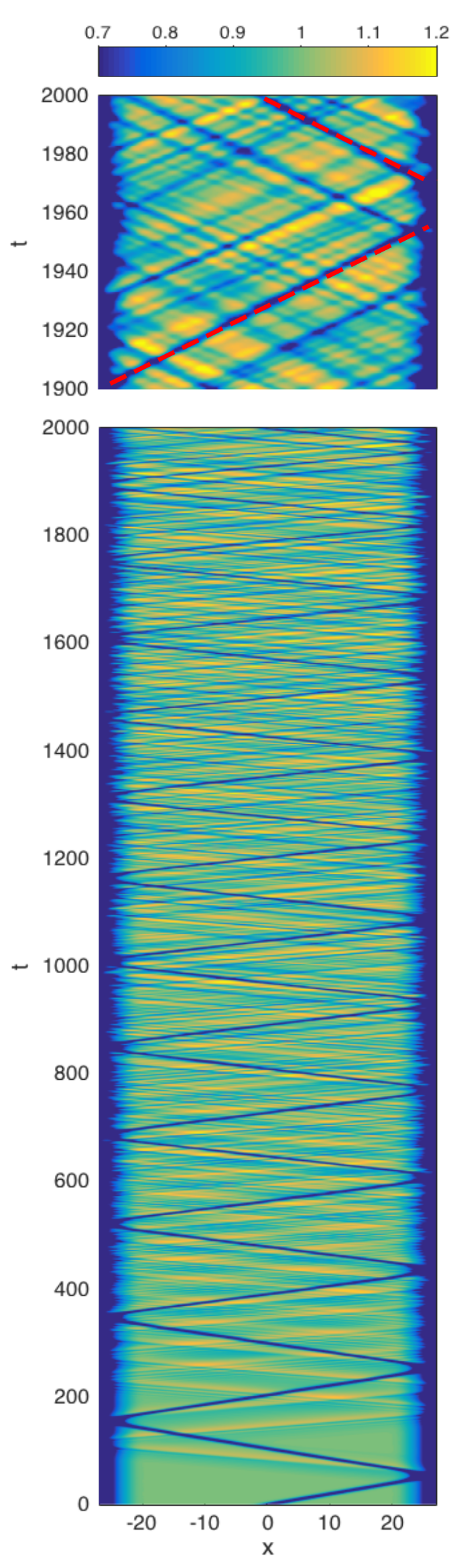
Figure 6: Dark soliton (initial speed $v=0.5$) oscillating in a power-law box trap. The upper plot shows a zoom-up over the time-range [1900,2000], with the original solition indicated by the dashed red line. Trap parameters $V_{0}=5$, $\alpha=2$, $L=40$ and $w=20$.

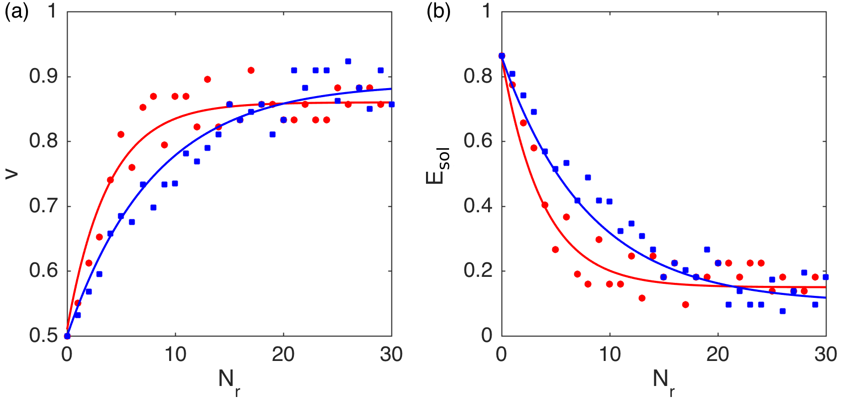
Figure 7: Decay of a soliton with initial speed $v=0.5$ after multiple reflections in a power-law trap. (a) Soliton speed after $N_{\rm r}$ reflections for $\alpha=1$ (red points) and $\alpha=2$ (blue data). The speed is measured as the average speed through the bulk of the condensate. (b) The soliton’s energy $E_{\rm sol}$, determined using the speed-energy relation (II.5). The solid lines are exponential fits to the data. Other parameters: $V_{0}=5$, $L=40$ and $w=20$.

To quantify the decay of the soliton during the repeated oscillations through the box we monitor the speed of the soliton through the bulk of the condensate following each reflection. Figure 7(a) shows the soliton speed versus the number of reflections $N_{\rm r}$ for two power-law boxes, while Fig. 7(b) shows the corresponding behaviour for the soliton’s energy, calculated using the energy-speed relation for a dark soliton (II.5). The qualitative behaviour is general: the soliton speed increases, relaxes towards a maximum value (which is less than unity), while the soliton’s energy decays towards a value (which exceeds zero). The trends are captured by an exponential fit (solid lines). Importantly, these results shows that the soliton does not decay away completely, but saturates towards a high speed/low energy state. By these late times, the system is full of density waves of similar amplitude, suggesting that the decay may be stabilized by absorption of energy from the density waves.

IV Discussion

We have seen that the reflection of the dark soliton from a soft wall is typically dissipative, in that the soliton loses energy through the emission of sound waves. An explanation of the partial reflection of the soliton can be found in the context of the propagation of optical pulses in an optical fiber. Indeed, the evolution equation of a dark solition in a normal-dispersion optical fiber is the so-called nonlinear Schrödinger equation, which is essentially the Gross-Pitaevskii equation (II.2) with time and spatial coordinates inverted. It is known there that the propagation of dark soliton is guaranteed thanks to the balancing between the linear term $u_{xx}$ (dispersion relation) and the nonlinear term $|u|^{2}u$ (self-phase modulation), as it occurs in our experiments where $V(x)=0.$ When the soliton approaches the potential wall, the balancing between the linear term $u_{xx}$ and $|u|^{2}u$ no longer occurs since the latter term now becomes $\left(|u|^{2}+V(x)\right)u$. In the optical context, the presence of $V(x)$ corresponds to a modification of the refractive index, which is equivalent to say that some energy of the soliton is supplied to generate some harmonic waves which travel faster than all the harmonic waves making their “envelope”, that is, the dark soliton wave.

To make more evident how the potential $V(x)$ modifies the mechanism of “spectral broadening” of the dark soliton caused by nonlinearity, we consider equation (II.2) without the dispersion term $u_{xx}$ (which is responsible only for the dispersion mechanism). The wave solution is then straightforward to find, and it takes the form $u(x,t)=|u(x,0)|\exp({\textrm{i}}\phi)$ with the phase $\phi=(|u(x,0)|^{2}+V(x))t$ depending also on $x$, which implies that the instantaneous wavenumber $\kappa$ differs across the wave from the central value. In Figs. 8 and 9 we show how the wavenumbers $\kappa$ of the dark soliton are shifted by the nonlinearity and the potential wall by plotting $\partial\phi/\partial x$ for $\alpha=2$ and $\alpha=0.001$ when the dark soliton approaches the potential wall. The dot-dashed red line refers to the absence of potential (which occurs in the central region of the BEC), while the blue line to the presence of the potential wall in the region between $w$ and $L$. Note that for $\alpha=0.001$ (Fig. 9) the two curves perflectly match, namely the potential wall does not affect the dark soliton which keeps on running undisturbed. However, for $\alpha=2$ (Fig. 8) the potential strongly modifies the instantaneous wavenumber $\kappa$, shifting it upwards and causing a different distribution of the energy (energy is supplied to other harmonics which run away from the soliton).

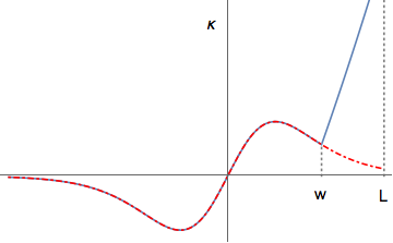
Figure 8: The instantaneous wavenumber $\kappa$ versus the $x$ axis for $\alpha=2$. The dot-dashed red line refers to $V(x)=0$, whereas the blue one to $V(x)\sim x^{2}$. The black solid line focus the center of the dark soliton and the dashed grey lines, instead, mark the region where the potential takes place.

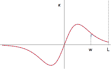
Figure 9: The same configuration used in Fig. 8 with $\alpha=0.001$.

As shown in Figures 2, 3 and 6, after the interaction of the soliton with the side of the potential, the “new” dark soliton (with lower energy and higher speed) enters again in the region with null potential, where the GP is completely integrable. The important issue here is that GP (II.2) admits the solution (II.4) for any $k$, namely the “new” dark soliton (just recovered from the side) may propagate undisturbed again in the BEC without any loss and showing its main features, as for instance to keep its identity after a collision with the other waves (in our case, the sound waves).

Over multiple oscillations in the box-like trap, the energy loss and speed increase of the soliton (which is very small for a single reflection) can become significant. With each reflection the condensate becomes increasingly populated with dispersive density waves, which are soon well-distributed through the condensate. This procedure lasts untill the density depth $k$ of the soliton is comparable to the amplitude of these dispersive waves (see Fig. 6). It is then hard to distinguish the residual dark soliton from the overlapping waves (see the top of Fig. 6), causing two complications. Firstly, the evaluation of the speed or energy of the soliton becomes affected by these waves overlapping the soliton (causing the scatter in the points in Fig. 7). Secondly, the interaction of the soliton with these dispersive waves cannot be neglected, even though the soliton keeps its identity after the reflections Oreshnikov-OL2015 . Indeed, density waves (sound) can supply energy back to some harmonics of the soliton, enhancing its energy.

V Conclusions

We have studied the propagation of dark solitons in 1D zero-temperature Bose-Einstein condensates confined by box-like external potentials consisting of a central flat region where the condensate is pratically free and two “soft” walls (power-law or Gaussian) of variable height and steepness. In the central region the one-dimensional GP is completely integrable, and dark solitons propagate undisturbed. When a soliton meets a side of the trap, depending on the steepness, the soliton may experience total or partial reflection. In the case of partial reflection, small amplitude density waves (sound) are generated and carry energy away from the soliton, and the soliton’s speed increases slightly. We map this energy loss as a function of the wall parameters. The reflection is perfect for almost vertical sides. In the dissipative regime and for multiple reflections, the soliton’s decay becomes significant. The condensate becomes increasingly populated by dispersive density waves and when the soliton’s depth reaches the level of these waves, its decay stabilizes. Finally, we can conclude that the stability and dynamics of dark solitons in box-like traps is fundamentally distinct from that in the well-studied case of harmonic potentials, where the soliton is established to propagate with no net dissipation.

References

- (1) Y. S. Kivshar and B. Luther-Davies, Phys. Rep. 278, 81 (1998).
- (2) P. Emplit, J.P. Hamaide, F. Reynaud, C. Froehly, and A. Barthelemy, Optics Comm. 62, 374 (1987).
- (3) D. Krökel, N. J. Halas, G. Giuliani, and D. Grischkowsky, Phys. Rev. Lett. 60, 29 (1988).
- (4) A. M. Weiner, J. P. Heritage, R. J. Hawkins, R. N. Thurston, E. M. Kirschner, D. E. Leaird, and W. J. Tomlinson, Phys. Rev. Lett. 61, 2445 (1988).
- (5) M. Chen, M. A. Tsankov, J. M. Nash and C. E. Patton, Phys. Rev. Lett. 70, 1707 (1993)
- (6) R. Heidemann, S. Zhdanov, R. Sütterlin, H. M. Thomas, and G. E. Morfill, Phys. Rev. Lett., 102, 135002 (2009).
- (7) E. Smirnov, C. E. Rüter, M. Stepić, D. Kip, and V. Shandarov, Phys. Rev. E 74, 065601 (2006).
- (8) A. Chabchoub, O. Kimmoun, H. Branger, N. Hoffmann, D. Proment, M. Onorato, and N. Akhmediev, Phys. Rev. Lett. 110, 124101 (2013).
- (9) D J Frantzeskakis, J. Phys. A 43, 213001 (2010).
- (10) S. Stenholm, Phys. Rep. 363, 173 (2002).
- (11) R. Carretero-González, D. J. Frantzeskakis, and P. G. Kevrekidis, Nonlinearity 21, R139 (2008).
- (12) E. P. Gross, Il Nuovo Cimento (1955-1965) 20, 454 (1961).
- (13) E. P. Gross, J. Math. Phys. 4, 195 (1963).
- (14) LP Pitaevskii, J. Exp. Theor. Phys. 13, 451 (1961).
- (15) S. Burger, K. Bongs, S. Dettmer, W. Ertmer, K. Sengstock, A. Sanpera, G. V. Shlyapnikov, and M. Lewenstein, Phys. Rev. Lett. 83, 5198 (1999).
- (16) J. Denschlag, J. E. Simsarian, D. L. Feder, C. W. Clark, L. A. Collins, J. Cubizolles, L. Deng, E. W. Hagley, K. Helmerson, W. P. Reinhardt, S. L. Rolston, B. I. Schneider, W. D. Phillips, Science 287, 97 (2000).
- (17) Z. Dutton, M. Budde, C. Slowe and L. V. Hau, Science 293, 663 (2001).
- (18) G.-B. Jo, J.-H. Choi, C. A. Christensen, T. A. Pasquini, Y.-R. Lee, W. Ketterle, and D. E. Pritchard, Phys. Rev. Lett. 98, 180401 (2007).
- (19) P. Engels and C. Atherton, Phys. Rev. Lett. 99, 160405 (2007).
- (20) C. Becker, S. Stellmer, P. S.-Panahi, S. Dörscher, M. Baumert, E.-M. Richter, J. Kronjäger, K. Bongs, and K. Sengstock, Nat. Phys. 4, 496 (2008).
- (21) J. J. Chang, P. Engels and M. A. Hoefer, Phys. Rev. Lett. 101, 170404 (2008).
- (22) S. Stellmer, C. Becker, P. Soltan-Panahi, E.-M. Richter, S. Dörscher, M. Baumert, J. Kronjäger, K. Bongs, and K. Sengstock, Phys. Rev. Lett. 101, 120406 (2008).
- (23) A. Weller, J. P. Ronzheimer, C. Gross, J. Esteve, M. K. Oberthaler, D. J. Frantzeskakis, G. Theocharis, and P. G. Kevrekidis, Phys. Rev. Lett. 101, 130401 (2008).
- (24) L. M. Aycock, H. M. Hurst, D. Genkina, H.-I. Lu, V. Galitski and I. B. Spielman, arXiv:1608.03916 (2016).
- (25) W. P. Reinhardt and C. W. Clark, J. Phys. B 30, L785 (1997).
- (26) Th. Busch and J. R. Anglin, Phys. Rev. Lett. 84, 2298 (2000).
- (27) G. Huang, J. Szeftel and S. Zhu, Phys. Rev. A 65, 053605 (2002).
- (28) N. G. Parker, N. P. Proukakis, M. Leadbeater and C. S. Adams, Phys. Rev. Lett. 90, 220401 (2003).
- (29) D. E. Pelinovsky, D. J. Frantzeskakis and P. G. Kevrekidis, Phys. Rev. E 72, 016615 (2005)
- (30) N. G. Parker, N. P. Proukakis and C. S. Adams, Phys. Rev. A 81, 033606 (2010).
- (31) D. E. Pelinovsky, Y. S. Kivshar and V. V. Afanasjev, Phys. Rev. E 54, 2015 (1996).
- (32) P. O. Fedichev, A. E. Muryshev, and G. V. Shlyapnikov, Phys. Rev. A 60, 3220 (1999).
- (33) A. E. Muryshev, G. V. Shlyapnikov, W. Ertmer, K. Sengstock and M. Lewenstein, Phys. Rev. Lett. 89, 110401 (2002).
- (34) B. Jackson, N. P. Proukakis and C. F. Barenghi, Phys. Rev. A 75, 051601(R) (2007).
- (35) G. Theocharis, P. G. Kevrekidis, M. K. Oberthaler and D. J. Frantzeskakis, Phys. Rev. A 76, 045601 (2007).
- (36) A. E. Muryshev, H. B. van Linden van den Heuvell, and G. V. Shlyapnikov, Phys. Rev. A 60, R2665 (1999).
- (37) L. D. Carr, M. A. Leung and W. P. Reinhardt, J. Phys. B: At. Mol. Opt. Phys. 33, 3983 (2000).
- (38) D. L. Feder, M. S. Pindzola, L. A. Collins, B. I. Schneider and C. W. Clark, Phys. Rev. A 62, 053606 (2000).
- (39) B. P. Anderson et al., Phys. Rev. Lett. 86, 2926 (2001).
- (40) M. A. Hoefer and B. Ilan, Phys. Rev. A 94, 013609 (2016).
- (41) N. G. Parker, N. P. Proukakis, M. Leadbeater and C. S. Adams, J. Phys. B 36, 2891 (2003).
- (42) A. J. Allen, D. P. Jackson, C. F. Barenghi and N. P. Proukakis, Phys. Rev. A 83, 013613 (2011).
- (43) P. G. Kevrekidis, R. Carretero-Gonzalez, G. Theocharis, D. J. Frantzeskakis, and B. A. Malomed, Phys. Rev. A 68, 035602 (2003).
- (44) N. G. Parker et al. J. Phys. B 37, S175 (2004).
- (45) D. J. Frantzeskakis et al., Phys. Rev. A 66, 053608 (2002).
- (46) N. P. Proukakis, N. G. Parker, D. J. Frantzeskakis and C. S. Adams, J. Opt. B 6, S380 (2004).
- (47) A. Radouani, Phys. Rev. A 68, 043620 (2003).
- (48) A. Radouani, Phys. Rev. A 70, 013602 (2004).
- (49) N. Bilas and N. Pavloff, Phys. Rev. A 72, 033618 (2005).
- (50) I. Hans, J. Stockhofe, and P. Schmelcher, Phys. Rev. A 92, 013627 (2015).
- (51) N. Bilas and N. Pavloff, Phys. Rev. Lett. 95, 130403 (2005)
- (52) T. P. Meyrath, F. Schreck, J. L. Hanssen, C.-S. Chuu, M. G. Raizen, Phys. Rev. A 71, 041604(R) (2005).
- (53) J. J. P. van Es, P. Wicke, A. H. van Amerongen, C. Rétif, S. Whitlock and N. J. van Druten, J. Phys. B 43, 155002 (2010)
- (54) L. Chomaz, L. Corman, T. Bienaime, R. Desbuquois, C. Weitenberg, S. Nascimbene, J. Beugnon and J. Dalibard, Nat. Comm. 6, 6162 (2015).
- (55) A.L. Gaunt, T.F. Schmidutz, I. Gotlibovych, R.P. Smith and Z. Hadzibabic, Phys. Rev. Lett. 110, 200406 (2013).
- (56) T. Brugarino and M. Sciacca, J. Math. Phys. 51, 093503 (2010).
- (57) C. F. Barenghi and N. G. Parker, “A Primer on Quantum Fluids” (Springer, Berlin, 2016)
- (58) I. Oreshnikov, R. Driben, and A.V. Yulin. Opt. Lett. 40, 4871 (2015).