Nonequilibrium phase behaviour from minimization of free power dissipation

Abstract

We develop a general theory for describing phase coexistence between nonequilibrium steady states in Brownian systems, based on power functional theory (M. Schmidt and J.M. Brader, J. Chem. Phys. 138, 214101 (2013)). We apply the framework to the special case of fluid-fluid phase separation of active soft sphere swimmers. The central object of the theory, the dissipated free power, is calculated via computer simulations and compared to a simple analytical approximation. The theory describes well the simulation data and predicts motility-induced phase separation due to avoidance of dissipative clusters.

Phase transitions in soft matter occur both in equilibrium and in nonequilibrium situations. Examples of the latter type include the glass transition weeks , various types of shear-banding instabilities observed in colloidal suspensions schall ; dhont , shear-induced demixing in semidilute polymeric solutions onuki , and motility-induced phase separation in assemblies of active particles phaseSeparationPapers ; CatesTailleurReview . In contrast to phase transitions in equilibrium, which obey the statistical mechanics of Boltzmann and Gibbs, very little is known about general properties of transitions between out-of-equilibrium states. A corresponding universal framework for describing nonequilibrium soft matter is lacking at present.

Theoretical progress has recently been made for the case of many-body systems governed by overdamped Brownian dynamics, encompassing a broad spectrum of physical systems Hansen06 . It has been demonstrated that the dynamics of such systems can be described by a unique time-dependent power functional $R_{t}[\rho,{\bf J}]$, where the arguments are the space- and time-dependent one-body density distribution, $\rho({\mathbf{r}},t)$, and the one-body current distribution, ${\bf J}({\mathbf{r}},t)$, in the case of a simple substance power ; brader13noz . Both these fields are microscopically sharp and act as trial variables in a variational theory. The power functional theory is regarded to be “important, [as it] provides (i) a rigorous framework for formulating dynamical treatments within the [density functional theory] formalism and (ii) a systematic means of deriving new approximations” EvansEtAl2016Preface .

The physical time evolution is that which minimizes $R_{t}[\rho,{\bf J}]$ at time $t$ with respect to ${\bf J}({\mathbf{r}},t)$, while keeping $\rho({\mathbf{r}},t)$ fixed. Hence

$$\frac{\delta R_{t}[\rho,{\bf J}]}{\delta{\bf J}({\mathbf{r}},t)} =0$$ (1)

at the minimum of the functional. Here the variation is performed at fixed time $t$ with respect to the position-dependent current. The density distribution is then obtained from integrating the continuity equation, $\partial\rho({\mathbf{r}},t)/\partial t=-\nabla\cdot{\bf J}({\mathbf{r}},t)$, in time. The power functional possesses units of energy per time, and can be split according to

$$R_{t}[\rho,{\bf J}]=P_{t}[\rho,{\bf J}]+\dot{F}[\rho]-X_{t}[\rho,{\bf J}],$$ (2)

where $P_{t}[\rho,{\bf J}]$ accounts for the irreversible energy loss due to dissipation, $\dot{F}[\rho]$ is the total time derivative of the intrinsic (Helmholtz) free energy density functional evans79 ; Hansen06 , and $X_{t}[\rho,{\bf J}]$ is the external power, given by

$$X_{t}[\rho,{\bf J}] =\int d{\mathbf{r}}[{\bf J}({\mathbf{r}},t)\cdot{\bf F}_{\rm ext}({\mathbf{r}},t)-\rho({\mathbf{r}},t)\dot{V}_{\rm ext}({\mathbf{r}},t)],$$ (3)

where $\dot{V}_{\rm ext}({\mathbf{r}},t)$ is the partial time derivative of the external potential $V_{\rm ext}({\mathbf{r}},t)$, and ${\bf F}_{\rm ext}({\mathbf{r}},t)$ is the external one-body force field, which in general consists of a sum of a conservative contribution, $-\nabla V_{\rm ext}({\mathbf{r}},t)$, and a further non-conservative term. The power dissipation is conveniently split into ideal and excess (above ideal) contributions: $P_{t}[\rho,{\bf J}]=P_{t}^{\rm id}[\rho,{\bf J}]+P_{t}^{\rm exc}[\rho,{\bf J}]$, where $P_{t}^{\rm exc}[\rho,{\bf J}]$ is nontrivial and arises from the internal interactions between the particles. The exact free power dissipation of the ideal gas is local in time and space and given by

$$P_{t}^{\rm id}[\rho,{\bf J}]=\frac{\gamma}{2}\int d{\mathbf{r}}\frac{{\bf J}({\mathbf{r}},t)^{2}}{\rho({\mathbf{r}},t)},$$ (4)

where $\gamma$ is the friction constant of the Brownian particles against the (implicit) solvent. This framework is formally exact and goes beyond dynamical density functional theory evans79 ; marinibettolomarconi99 ; archer04ddft ; the latter follows from neglecting the excess dissipation, $P_{t}^{\rm exc}[\rho,{\bf J}]=0$.

In this Letter we apply the general framework of power functional theory to treat phase coexistence of nonequilibrium steady states. Such a state of $N$ particles in a volume $V$ at temperature $T$ is characterized by a value of the total power functional taken at the (local) minimum, $R_{t}^{0}(N,V,T)\equiv R_{t}[\rho^{0},{\bf J}^{0}]$, where the superscript 0 indicates a quantity at the minimum. We define the chemical power derivative $\nu$ and the (negative) volumetric power derivative $\pi$ via partial differentiation,

$$\nu=\left.\frac{\partial R_{t}^{0}}{\partial N}\right|_{V,T},\quad\pi =-\left.\frac{\partial R_{t}^{0}}{\partial V}\right|_{N,T},$$ (5)

where $\nu$ and $\pi$ possess units of energy per time and pressure per time, respectively. In the limit of large $N$ and large $V$, the specific free power per volume, $r_{t}(\rho_{b})=R_{t}^{0}/V$, will depend only on the (bulk) number density $\rho_{b}=N/V$; this implies the identity $R_{t}^{0}=-\pi V+\nu N$, which neglects possible surface contributions. The simple relations $\nu=\partial r_{t}/\partial\rho_{b}$ and $\pi=-r_{t}+\rho_{b}\nu$ follow straightforwardly. We shall demonstrate below that the free power density, $r_{t}(\rho_{b})$, is the relevant physical quantity for analyzing phase behavior out-of-equilibrium.

We assume that two coexisting nonequilibrium steady states, $A$ and $B$, are characterized by particle number $N_{A}$ and $N_{B}$ and by volume $V_{A}$ and $V_{B}$, respectively. The density in phase A (B) is $\rho_{A}=N_{A}/V_{A}$ ($\rho_{B}=N_{B}/V_{B}$). Hence, in a phase separated state, the total power is a weighted sum,

$$R_{t}^{0}=r_{t}(\rho_{A})V_{A}+r_{t}(\rho_{B})V_{B},$$ (6)

where the partial volumes of the two phases are $V_{A}/V=(\rho_{B}-\rho_{b})/(\rho_{B}-\rho_{A})$ and $V_{B}/V=(\rho_{b}-\rho_{A})/(\rho_{B}-\rho_{A})$, with $\rho_{A}\leq\rho_{b}\leq\rho_{B}$.

The task of finding a global minimum of $R_{t}[\rho,{\bf J}]$ can now be facilitated by a Maxwell common tangent construction on $r_{t}(\rho_{b})$, which implies the identities

$$r_{t}^{\prime}(\rho_{A}) =r_{t}^{\prime}(\rho_{B})=\frac{r_{t}(\rho_{B})-r_{t}(\rho_{A})}{\rho_{B}-\rho_{A}},$$ (7)

where $r_{t}^{\prime}(\rho_{b})=\partial r_{t}(\rho_{b})/\partial\rho_{b}$. As a consequence, both the chemical and the volumetric derivatives have the same value in the coexisting phases:

$$\nu_{A} =\nu_{B},\quad\pi_{A}=\pi_{B},$$ (8)

and equality of temperature is trivial by construction.

In order to illustrate this framework, we apply it to treat active Brownian particles, which form a class of systems attracting much current interest CatesAndCompany1a ; CatesAndCompany1b ; CatesAndCompany2 ; phaseSeparationPapers . We consider spherical particles in $d$-dimensional space, with position coordinates ${\mathbf{r}}^{N}\equiv\{{\mathbf{r}}_{1}\ldots{\mathbf{r}}_{N}\}$ and (unit vector) orientations $\boldsymbol{\omega}^{N}\equiv\{\boldsymbol{\omega}_{1}\ldots\boldsymbol{\omega}_{N}\}$; here the orientational motion of each ${\boldsymbol{\omega}}_{i}$, where $i=1\ldots N$, is freely diffusive with orientational diffusion constant $D_{\rm rot}$. The swimming is due to an orientation-dependent external force field, ${\bf F}_{\rm ext}({\boldsymbol{\omega}}_{i})=\gamma s{\boldsymbol{\omega}}_{i}$, which is nonconservative and does not depend explicitly on ${\mathbf{r}}$ and $t$; here $s$ is the speed for free swimming. We follow Refs. CatesAndCompany1a ; CatesAndCompany1b and use the Weeks-Chandler-Andersen model, i.e., a Lennard-Jones pair potential, which is cut and shifted at its minimum, such that the resulting short-ranged pair force is continuous and purely repulsive. For numerical convenience our Brownian dynamics (BD) simulations will be performed in $d=2$.

Power functional theory provides a microscopic many-body expression for $R_{t}^{0}$ power . Omitting an irrelevant rotational contribution, this is given (up to a constant $C$) by

$$R_{t}^{0}=-\frac{\gamma}{2}\langle\sum_{i}{\bf v}_{i}(t)^{2}\rangle+C,$$ (9)

where the sum is over all particles and the angles denote a steady state average. To directly simulate the dissipated free power, we use a discretized version of the instantaneous velocity fortini14prl , ${\bf v}_{i}(t)=({\mathbf{r}}_{i}(t+\Delta t)-{\mathbf{r}}_{i}(t-\Delta t))/(2\Delta t)$, where $\Delta t$ is the time step of the standard (Euler) computer simulation algorithm, where ${\mathbf{r}}_{i}(t+\Delta t)={\mathbf{r}}_{i}(t)+\gamma^{-1}\Delta t[-\nabla_{i}U({\mathbf{r}}^{N})+\boldsymbol{\xi}_{i}(t)+{\bf F}_{\rm ext}({\boldsymbol{\omega}}_{i}(t))]$, with $\boldsymbol{\xi}_{i}(t)$ being a Gaussian-distributed delta-correlated noise term, with finite-difference, equal-time strength $\langle\boldsymbol{\xi}_{i}(t)\cdot\boldsymbol{\xi}_{j}(t)\rangle=\delta_{ij}k_{B}Td/(\gamma\Delta t)$; $C=Nk_{B}Td/(2\Delta t)$ is an irrelevant constant, and $k_{B}$ is the Boltzmann constant. The external power is given by

$$X_{t} =\langle\sum_{i}{\bf v}_{i}(t)\cdot{\bf F}_{\rm ext}({\boldsymbol{\omega}}_{i}(t))\rangle,$$ (10)

and we define the corresponding internal power, due to interparticle interactions and Brownian forces, as

$$I_{t}=\langle\sum_{i}{\bf v}_{i}(t)\cdot(-\nabla_{i}U({\mathbf{r}}^{N})+{\boldsymbol{\xi}}_{i}(t))\rangle.$$ (11)

This allows us to split (9) into a sum of external and internal contributions,

$$R_{t}^{0}=-I_{t}/2-X_{t}/2.$$ (12)

By inserting (2) into (1) and observing the structure of (4), it is straightforward to show that

$$I_{t}=-\dot{F}-2P_{t}^{\rm exc}+\int d{\mathbf{r}}d{\boldsymbol{\omega}}{\bf J}({\mathbf{r}},{\boldsymbol{\omega}},t)\cdot\left.\frac{\delta P_{t}^{\rm exc}[\rho,{\bf J}]}{\delta{\bf J}({\mathbf{r}},{\boldsymbol{\omega}},t)}\right|_{0},$$ (13)

where the integrand is evaluated at the minimum, and we included the argument ${\boldsymbol{\omega}}$, treating the system effectively as a mixture of different components brader14tpl .

To sample (9) efficiently in simulation, we decompose the velocity as ${\bf v}_{i}(t)=(\Delta{\mathbf{r}}_{i}(t-\Delta t)+\Delta{\mathbf{r}}_{i}(t))/(2\Delta t)$, where $\Delta{\mathbf{r}}_{i}(t)={\mathbf{r}}_{i}(t+\Delta t)-{\mathbf{r}}_{i}(t)$, given via the Euler algorithm as a sum of three contributions, i.e., intrinsic, $\Delta{\mathbf{r}}_{i}^{\rm int}(t)=-\Delta t\nabla_{i}U({\mathbf{r}}^{N}(t))$; random, $\Delta{\mathbf{r}}_{i}^{\rm ran}(t)=\Delta t\boldsymbol{\xi}_{i}(t)$; and external, $\Delta{\mathbf{r}}_{i}^{\rm ext}(t)=\Delta t{\bf F}_{\rm ext}({\boldsymbol{\omega}}_{i}(t))$. Multiplying out (9) yields 36 contributions, of which we only sample the three non-trivial types: $\langle\Delta{\mathbf{r}}_{i}^{\rm int}(t)\cdot\Delta{\mathbf{r}}_{i}^{\rm int}(t)\rangle$ and $\langle\Delta{\mathbf{r}}_{i}^{\rm int}(t)\cdot\Delta{\mathbf{r}}_{i}^{\rm ext}(t)\rangle$ (where also similar contributions arise with one or both displaced time arguments), as well as $\langle\Delta{\mathbf{r}}_{i}^{\rm ran}(t-\Delta t)\cdot\Delta{\mathbf{r}}_{i}^{\rm int}(t)\rangle$. We use $N=1000$ and adjust $V$ in order to control the density in the square simulation box with periodic boundaries. The time step is chosen as $\Delta t/\tau_{0}=10^{-5}$, where the timescale is $\tau_{0}=\gamma\sigma^{2}/\epsilon$, with Lennard-Jones diameter $\sigma$ and energy scale $\epsilon$. We allow the system to reach a steady state in $10^{7}$ steps, and collect data for a further $10^{8}$ steps. The rotational diffusion constant is set to $D_{\rm rot}=3k_{B}T/(\gamma\sigma^{2})$, and the external field strength is chosen as $s=24\sigma/\tau_{0}$. The Peclet number CatesAndCompany1a ; CatesAndCompany1b is ${\rm Pe}\equiv 3s/(D_{\rm rot}\sigma)=\gamma s\sigma/(k_{B}T)$.

Figure 1(a) shows simulation results for $R_{t}^{0}$ and $X_{t}$, as respectively given by (9) and (10), as a function of density. Due to the simple form of the external force, the external power (10) is trivially related to the (well-studied CatesAndCompany1a ; CatesAndCompany1b ; CatesAndCompany2 ) average forward swimming speed $v$ via $X_{t}=\gamma svN$, where $v=\langle\sum_{i}{\bf v}_{i}(t)\cdot{\boldsymbol{\omega}}_{i}\rangle/N$. Remarkably, we find that $R_{t}^{0}$ coincides with $-X_{t}/2$ within our numerical precision. This implies that (i) the internal dissipation is negligible, $I_{t}\approx 0$ (cf. (12)) and (ii) that the value of the power functional for active particles is a known quantity. We have systematically studied the variation with temperature (as is analogous to varying Pe CatesAndCompany1a ; CatesAndCompany1b ). While hardly any effect for low densities is observed, a dip develops for $\rho\sigma^{2}\gtrsim 0.5$, cf. Fig. 1a footnoteStenhammar .

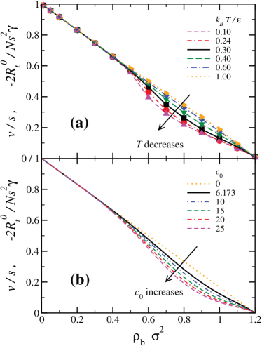
Figure 1: (a) Scaled average forward swimming speed $v/s$ (symbols) and scaled free power $-2R_{t}^{0}/(Ns^{2}\gamma)$ per particle (lines), as obtained from BD computer simulations via Eqs. (9) and (10), respectively, for temperatures $k_{B}T/\epsilon=0.1$–1 (as indicated). (b) Theoretical results corresponding to (a), as given by Eqs. (17) and (19), where $m=5$, $\rho_{0}\sigma^{2}=1.2$, and for values of $c_{0}=0$–25 as indicated.

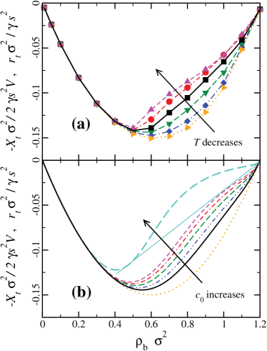
Figure 2: The same as Fig. 1, but scaled per volume $V$, rather than per particle $N$; the conversion factor is $-2V/\sigma^{2}$, such that $r_{t}\sigma^{2}/(\gamma s^{2})$ and $-X_{t}\sigma^{2}/(2\gamma s^{2}V)$ are shown as a function of $\rho_{b}\sigma^{2}$. The straight line in (b) indicates the double tangent for the case $c_{0}=100$; the black solid line indicates the result at the critical value of $c_{0}$.

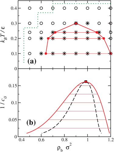
Figure 3: (a) Phase diagram for active particles, obtained from simulations, as a function of scaled density $\rho_{b}\sigma^{2}$ and scaled temperature $k_{B}T/\epsilon$. Shown are the binodal (red solid line) obtained from double tangent construction (red filled symbols), horizontal tielines (thin red lines), and estimate for the critical point (red square). Also shown are single-phase (open symbols) and phase-separated (stars) states based on analysis of the decay of $g(r)$. The phase boundary of Ref. CatesAndCompany1a ; CatesAndCompany1b is also shown (green dotted line). (b) Same as (a), but obtained from power functional theory, and shown as a function $1/c_{0}$ instead of scaled temperature. The dashed line indicates the spinodal.

We next seek to develop a simple theoretical model to capture the key features of the simulation data; the corresponding results shown in Fig. 1(b) will be discussed below. We assume $P_{t}^{\rm exc}[\rho,{\bf J}]$ to possess a simple Markovian, spatially nonlocal form:

$$P_{t}^{\rm exc}[\rho,{\bf J}] =\frac{\gamma}{2}\int\!d1\!\!\int\!d2\,\rho(1)\rho(2)\left(\frac{{\bf J}(1)}{\rho(1)}-\frac{{\bf J}(2)}{\rho(2)}\right)^{2}\!M(1,2),$$ (14)

where $1\equiv{\mathbf{r}},{\boldsymbol{\omega}}$ and $2\equiv{\mathbf{r}}^{\prime},{\boldsymbol{\omega}}^{\prime}$. Here $M(1,2)$ is a (dimensionless) correlation kernel that couples the particles at points 1 and 2, similar to the mean-field form of the excess free energy functional in equilibrium density functional theory Hansen06 ; evans79 . Note that the term in brackets in (14) is the (squared) velocity difference between the two points. We parameterize the current, which in general depends on particle position ${\mathbf{r}}$ and orientation ${\boldsymbol{\omega}}$, as ${\bf J}({\mathbf{r}},{\boldsymbol{\omega}},t)=J_{b}{\boldsymbol{\omega}}$, where the $J_{b}$ is a variational parameter that determines the (homogeneous) bulk current in direction ${\boldsymbol{\omega}}$. This implies $v=J_{b}/\rho_{b}$. Inserting into (14) and observing the general structure (2), we obtain

$$\frac{R_{t}}{\gamma V} =\frac{J_{b}^{2}}{2\rho_{b}}+\frac{M_{0}}{2}J_{b}^{2}-sJ_{b},$$ (15)

where the right hand side consists of a sum of contributions due to ideal dissipation ($P_{\rm id}$), excess contribution to dissipation ($P_{\rm exc}$) and external power ($X_{t}$). The coefficient $M_{0}$ is density-dependent and can be expressed as a moment of the correlation kernel brader13noz $M(1,2)$, as $M_{0}=\int d{\mathbf{r}}d{\boldsymbol{\omega}}d{\boldsymbol{\omega}}^{\prime}({\boldsymbol{\omega}}-{\boldsymbol{\omega}}^{\prime})^{2}M(1,2)$, where due to symmetries $M(1,2)$ depends only on the differences ${\mathbf{r}}-{\mathbf{r}}^{\prime}$ and ${\boldsymbol{\omega}}-{\boldsymbol{\omega}}^{\prime}$, and $M_{0}$ is hence independent of ${\mathbf{r}}^{\prime}$. Clearly, in steady states $\dot{F}[\rho]=0$.

The minimization principle (1) implies $\partial R_{t}/\partial J_{b}=0$ for (15), which yields

$$J_{b} =s\rho_{b}/(1+M_{0}\rho_{b}).$$ (16)

Using (16) in order to eliminate $M_{0}$ from (15) gives the value at the minimum

$$R_{t}^{0} =-\gamma sJ_{b}V/2,$$ (17)

which implies that $R_{t}^{0}=-X_{t}/2$, where here the external power is $X_{t}=\gamma sJ_{b}V$. A detailed derivation will be given elsewhere. The internal contribution $I_{t}=0$, as $\dot{F}=0$ in steady state, and the additional contributions in (13) vanish for the present form (14) of $P_{\rm exc}[\rho,{\bf J}]$, which is quadratic in ${\bf J}({\mathbf{r}},{\boldsymbol{\omega}},t)$.

We assume a simple analytical expression,

$$M_{0} =(\rho_{0}-\rho_{b})^{-1}+c_{0}\rho_{b}^{m}/\rho_{0}^{m+1},$$ (18)

where $\rho_{0}$ is the jamming density at which the dynamics arrests, $c_{0}\geq 0$ is a temperature-dependent dimensionless constant, and the exponent $m>0$ is a measure for the number of particles that cause the additional dissipation due to local cluster formation (second term in (18)). We expect the exponent $m$ to grow with $d$, as clusters consist of an increasing number of particles upon increasing $d$. Furthermore, we expect $c_{0}$ to decrease to zero with increasing temperature, as clusters are broken up by thermal motion. We leave a microscopic derivation of $M_{0}$, e.g. starting from the correlation kernel $M(1,2)$ (which is in principle accessible e.g. via simulations schindler2016 ) to future work. Equation (18) can be interpreted as describing an overall increase, and eventual divergence, of dissipation with density plus a specific dissipation channel due to small groups of the order of $m$ particles that block each other. Blocking is only relevant at intermediate densities, high enough so that the $m$-th density order contributes, but low enough in order to be not overwhelmed by the singularity.

Inserting (18) into (16) yields

$$\frac{J_{b}}{s\rho_{b}} =\frac{1-x}{1+c_{0}x^{m+1}(1-x)},$$ (19)

where we have defined the scaled density $x=\rho_{b}/\rho_{0}$. In case of high temperature, where $c_{0}\to 0$, this reduces to the simple and well-known (see, e.g., CatesAndCompany1a ; CatesAndCompany1b ; CatesAndCompany2 ) linear (velocity) relationship $v/s\equiv J_{b}/(s\rho_{b})=1-x$. In Fig. 1(b), we show the theoretical results for the (scaled) external and total free power per particle corresponding to the simulation results in Fig. 1(a). Clearly, despite the simplicity of (18) the theory reproduces the simulation data very well.

As outlined above, in order to assess phase behavior, the relevant quantity is the free power per volume $r_{t}$ (rather than per particle), which we show in Fig. 2, obtained from simulations (Fig. 2(a)) and theory (Fig. 2(b)). For low temperatures $k_{B}T/\epsilon=0.1,0.24$, the simulation data clearly show a change in curvature, which we attribute to a first-order phase transition in the finite system footnoteSystemSize . (In an infinite system, we expect no negative curvature to occur, and the coexistence region to be characterized by a strictly linear variation of $r_{t}$ with $\rho_{b}$.) For $k_{B}T/\epsilon=0.3$ a quasilinear part can be observed, which we interpret as being very close to a nonequilibrium critical point. The theoretical curve displays the same type of behavior, which we attribute to the mean-field character of the approximation (14). We can now apply the general phase coexistence conditions (7) and (8) to the active system. A representative double tangent is shown in Fig. 2(b). The low-density (high-density) coexisting phase is characterized by high (low) value of $X_{t}$.

The phase diagram (cf. Fig. 3) displays two-phase coexistence between a high-density and a low-density active fluid. We find the simulation results (Fig. 3(a)) for the binodal obtained from double tangent construction (on the results shown above in Fig. 2(a)) as a function of $k_{B}T/\epsilon$ to be consistent with the behaviour of the tail ($5<r/\sigma<10$) of the radial pair distribution function $g(r)$. A characteristic slow decay indicates occurrence of phase separation (see, e.g., farage2015 ). The corresponding theoretical phase diagram is shown in Fig. 3(b), where we also display the spinodal, defined as the point(s) of inflection of $r_{t}(\rho_{b})$. The phase separation vanishes upon increasing $1/c_{0}$ at an upper nonequilibrium critical point. Although we have not attempted to model the dependence of $1/c_{0}$ on $T$ systematically, the agreement between simulation and theoretical results is striking. Our simulation results for the phase behaviour underestimate the boundaries given by Stenhammar et al. CatesAndCompany1a ; CatesAndCompany1b ; this is not surprising given that these authors investigated significantly larger systems. In simulations we have found only a slight decrease of the slope of $v(\rho_{b})$ for increasing $s$, and corresponding increase in the jamming density, but with little effect on the phase separation itself. This is consistent with the fact that $P_{\rm exc}[\rho,{\bf J}]$, and hence, $c_{0}$ is an intrinisic quantity. The conditions for spinodal and binodal both differ from the density “where macroscopic MIPS [mobility-induced phase separation] is initiated by spinodal decomposition” CatesTailleurReview , $v^{\prime}/v=-1/\rho_{b}$, where $v^{\prime}=dv(\rho_{b})/d\rho_{b}$; this can be rephrased as $d(\rho_{b}v)/d\rho_{b}=0$, implying, within $I_{t}=0$, that $r_{t}^{\prime}(\rho_{b})=0$. This condition is quite different from the spinodal within power functional theory, $r_{t}^{\prime\prime}(\rho_{b})=0$, or equivalently $v^{\prime\prime}/v^{\prime}=-2/\rho_{b}$. Furthermore, for linear variation of $v$ with $\rho_{b}$, i.e., $c_{0}=0$, we find phase separation to be absent, in contrast to Ref. CatesTailleurReview ; cf. Eqs.(35)-(37) and Fig. 5 therein.

We have developed a general approach, based on power functional theory power , to treat coexistence between nonequilibrium steady states in Brownian systems. Our theory is fundamentally different from other approaches to active systems (e.g. phaseSeparationPapers ; farage2015 ; furtherPapers ) which were developed specifically for phase separation. We rather identify a generating functional providing a unified, internally self-consistent description of out-of-equilibrium states. The free power density plays a role in nonequilibrium systems analogous to that of the free energy density in equilibrium, although it is an entirely distinct physical quantity.

References

- (1) G. L. Hunter and E. Weeks, Rep. Prog. Phys. 75, 066501 (2012).
- (2) V. Chikkadi, D. M. Miedema, M. T. Dang, B. Nienhuis, and P. Schall, Phys. Rev. Lett. 113, 208301 (2014).
- (3) J. K. G. Dhont, Faraday Discuss. 123, 157 (2003).
- (4) A. Onuki, Phase Transition Dynamics, (Cambridge University Press, Cambridge, 2002).
- (5) Y. Fily, S. Henkes and M. C. Marchetti, Soft Matter 10, 2132 (2014); J. Bialké, H. Löwen and T. Speck, EPL 103, 30008 (2013);
- (6) M. E. Cates and J. Tailleur, Annu. Rev. Condens. Matter Phys. 6, 219 (2015).
- (7) J. P. Hansen and I. R. McDonald, Theory of Simple Liquids, 4rd ed. (Academic Press, Amsterdam, 2013).
- (8) M. Schmidt and J. M. Brader, J. Chem. Phys. 138 214101 (2013).
- (9) J. M. Brader and M. Schmidt, J. Chem. Phys. 139, 104108 (2013).
- (10) R. Evans et al., J. Phys.: Condens. Matter 28, 240401 (2016).
- (11) R. Evans, Adv. Phys. 28, 143 (1979).
- (12) U. Marini Bettolo Marconi and P. Tarazona, J. Chem. Phys. 110, 8032 (1999).
- (13) A. J. Archer and R. Evans, J. Chem. Phys. 121, 4246 (2004).
- (14) J. Stenhammar, A. Tiribocchi, R. J. Allen, D. Marenduzzo, and M. E. Cates, Phys. Rev. Lett. 111, 145702 (2013);
- (15) J. Stenhammar, D. Marenduzzo, R. J. Allen and M. E. Cates, Soft Matter 10, 1489 (2014).
- (16) A. P. Solon, J. Stenhammar, R. Wittkowski, M. Kardar, Y. Kafri, M. E. Cates, and J. Tailleur, Phys. Rev. Lett. 114, 198301 (2015); A. P. Solon, Y. Fily, A. Baskaran, M. E. Cates, Y. Kafri, M. Kardar and J. Tailleur, Nat. Phys. 11, 673 (2015).
- (17) A. Fortini, D. de las Heras, J. M. Brader, M. Schmidt, Phys. Rev. Lett. 113, 167801 (2014). The trajectory-based velocity is analogous to the operator description of Refs. power ; brader13noz .
- (18) J. M. Brader and M. Schmidt, J. Phys.: Condens. Matter 27, 194106 (2015).
- (19) Nonlinear behaviour of simulation results for has been reported before, see Fig. S3 in the supplementary material of Ref. CatesAndCompany1a .
- (20) T. Schindler and M. Schmidt, J. Chem. Phys. 145, 064506 (2016).
- (21) We expect the precise form of and hence the value of the phase coexistence densities to be affected by finite size effects.
- (22) T. F. F. Farage, P. Krinninger, and J. M. Brader, Phys. Rev. E 91, 042310 (2015).
- (23) I. Theurkauff et al., Phys. Rev. Lett. 108, 268303 (2012); G. S. Redner et al., Phys. Rev. Lett. 110, 055701 (2013); I. Buttinoni et al., Phys. Rev. Lett. 110, 238301 (2013); G. S. Redner et al., arXiv:1603.01362 (2016); D. Richard et al., Soft Matter 12, 5257 (2016).