Abstract

$Q$-conditional symmetries (nonclassical symmetries) for the general class of two-component reaction-diffusion systems with non-constant diffusivities are studied. Using the recently introduced notion of $Q$-conditional symmetries of the first type, an exhausted list of reaction-diffusion systems admitting such symmetry is derived. The results obtained for the reaction-diffusion systems are compared with those for the scalar reaction-diffusion equations. The symmetries found for reducing reaction-diffusion systems to two-dimensional dynamical systems, i.e., ODE systems, and finding exact solutions are applied. As result, multiparameter families of exact solutions in the explicit form for a nonlinear reaction-diffusion system with an arbitrary diffusivity are constructed. Finally, the application of the exact solutions for solving a biologically and physically motivated system is presented.

2000 Mathematics Subject Classification : 35K50, 35K60, 22E70.

Keywords: nonlinear reaction-diffusion system, Lie symmetry, $Q$-conditional symmetry, non-classical symmetry, exact solution.

1 Introduction

The paper is devoted to the investigation of the two-component RD systems of the form

$$\begin{array}[]{l}U_{t}=[D^{1}(U)U_{x}]_{x}+F(U,V),\\ V_{t}=[D^{2}(V)V_{x}]_{x}+G(U,V),\end{array}$$ (1)

where $U=U(t,x)$ and $V=V(t,x)$ are two unknown functions representing the densities of populations (cells, chemicals), the pressures in thin films, etc. $F(U,V)$ and $G(U,V)$ are the given smooth functions describing interaction between them and environment, the functions $D^{1}(U)$ and $D^{2}(V)$ are the relevant diffusivities (hereafter they are positive smooth functions) and the subscripts $t$ and $x$ denote differentiation with respect to these variables. The class of RD systems (1) generalizes many well-known nonlinear second-order models and is used to describe various processes in physics, biology, chemistry and ecology (see, e.g., the well-known books [2, 3, 4, 5]). As a particular case, this system corresponds to a model for the chemical basis of morphogenesis proposed by Turing [6] and is called the interacting population diffusion system (for two species) [3, Section 9.2]. Usually the diffusivities $D^{k}\ (k=1,2)$ are taken to be positive constant, however, in certain insect dispersal models they depend on the densities $U$ and $V$, for example, a power dependence is adopted in [3, Section 11.4], [7], and [8].

During the last decades RD systems of the form (1) have been extensively studied by means of different mathematical methods, including the classical Lie method. The search of Lie symmetries of the class of RD systems (1) with constant diffusivities, i.e.

$$\begin{array}[]{l}U_{t}=d_{1}U_{xx}+F(U,V),\\ V_{t}=d_{2}V_{xx}+G(U,V)\end{array}$$ (2)

was initiated in the paper [9]. At present, one can claim that all possible Lie symmetries of (1) with the constant diffusivities are completely described [10, 11]. In the case of non-constant diffusivities, it has been done in [12], where 30 RD systems admitting non-trivial Lie algebras of invariance were found. It turns out that many of them are locally equivalent therefore those 30 systems can be reduced to 10 RD systems with non-trivial Lie symmetry [8]. In the paper [13], this result was extended on RD systems in the $(n+1)$ – dimensional Euclid space. Note that Lie symmetries of RD systems (2) with the linear cross-diffusion were described in [14].

In contrary to the Lie symmetry classification problem, one of $Q$-conditional symmetry classification for the class of RD systems (1) is not solved at the present time. To the best of our knowledge the most general result was derived in [15], where the $Q$-conditional symmetries (non-classical symmetries) of the subclass

$$\begin{array}[]{l}U_{t}=(U^{k}U_{x})_{x}+F(U,V),\\ V_{t}=(V^{l}V_{x})_{x}+G(U,V)\end{array}$$ (3)

where described (here $k$ and $l$ are real constants). Note that the result obtained therein is incomplete because the system of determining equations (16) [15] was solved only under additional restrictions. The main reason of such incompleteness follows from the structure of determining equations, which are essentially nonlinear in contrary to those in the case of the Lie symmetry classification problem. Thus, to solve $Q$-conditional symmetry classification problem for the class of RD systems (1), one should look for new constructive approaches helping to solve the relevant nonlinear system of determining equations. A possible approach was recently proposed in [16] and is used in this paper.

The paper is organized as follows. In section 2, two different definitions of $Q$-conditional invariance are presented, the system of determining equations is derived and the main theorem is proved. In section 3, the $Q$-conditional symmetries obtained for reducing of RD systems to systems of ODEs are applied and multiparameter families of exact solutions are constructed. An example of application of the exact solution obtained for solving a boundary value problem with the zero-flux conditions is presented, too. Finally, we summarize and discuss the results obtained in the last section.

2 Conditional symmetry for RD systems

2.1 Definitions and preliminary analysis

One notes that the RD system (1) can be simplified by applying the Kirchhoff substitution

$$u=\int D^{1}(U)dU,\quad v=\int D^{1}(V)dV,$$ (4)

where $u(t,x)$ and $v(t,x)$ are new unknown functions. Hereafter we assume that there exist unique inverse functions to those arising in right-hand-sides of (4). Substituting (4) into (1), one obtains

$$\begin{array}[]{l}u_{xx}=d^{1}(u)u_{t}+C^{1}(u,v),\\ v_{xx}=d^{2}(v)v_{t}+C^{2}(u,v),\end{array}$$ (5)

where the functions $d^{1},\ d^{2}$ and $C^{1},C^{2}$ are uniquely defined via $D^{1},\ D^{2}$ and $F,G$, respectively. In fact, the formulae

$$d^{1}(u)=\frac{1}{D^{1}(U)},\ d^{2}(v)=\frac{1}{D^{2}(V)},\ C^{1}(u,v)=-F(U,V),\ C^{2}(u,v)=-G(U,V),$$ (6)

where $U=D^{1}_{*}(u)\equiv\Bigl{(}\int D^{1}(u)du\Bigl{)}^{-1},\quad V=D^{2}_{*}(v)\equiv\Bigl{(}\int D^{2}(v)dv\Bigl{)}^{-1}$ (the upper subscripts $-1$ mean inverse functions). Hereafter we construct conditional symmetries for class of RD systems (5) instead of (1). Having any conditional symmetry operator of a RD system of the form (5), one may easily transform those into the relevant operator and a RD system from the class (1) provided the inverse functions in (6) are known.

Here we use the definition of $Q$-conditional symmetry of the first type introduced recently in [16] and applied successfully to search such symmetries for the classical Lotka-Volterra system [17].

It is well-known that to find Lie invariance operators, one needs to consider system (5) as the manifold ${\cal{M}}=\{S_{1}=0,S_{2}=0\}$ where

$$\begin{array}[]{l}S_{1}\equiv\ u_{xx}-d^{1}(u)u_{t}-C^{1}(u,v),\\ S_{2}\equiv\ v_{xx}-d^{2}(v)v_{t}-C^{2}(u,v),\end{array}$$ (7)

in the prolonged space of the variables: $t,x,u,v,u_{t},v_{t}$,$u_{x},v_{x},u_{xx},v_{xx},u_{xt},v_{xt},u_{tt},v_{tt}.$ According to the definition, system (5) is invariant under the transformations generated by the infinitesimal operator

$$Q=\xi^{0}(t,x,u,v)\partial_{t}+\xi^{1}(t,x,u,v)\partial_{x}+\eta^{1}(t,x,u,v)\partial_{u}+\eta^{2}(t,x,u,v)\partial_{v},$$ (8)

if the following invariance conditions are satisfied:

$$\begin{array}[]{l}\mbox{\raisebox{-4.73611pt}{$\stackrel{{\scriptstyle\displaystyle Q}}{{\scriptstyle 2}}$}}S_{1}\equiv\mbox{\raisebox{-4.73611pt}{$\stackrel{{\scriptstyle\displaystyle Q}}{{\scriptstyle 2}}$}}\big{(}u_{xx}-d^{1}(u)u_{t}-C^{1}(u,v)\big{)}\Big{|}_{\cal{M}}=0,\\[8.5359pt] \mbox{\raisebox{-4.73611pt}{$\stackrel{{\scriptstyle\displaystyle Q}}{{\scriptstyle 2}}$}}S_{2}\equiv\mbox{\raisebox{-4.73611pt}{$\stackrel{{\scriptstyle\displaystyle Q}}{{\scriptstyle 2}}$}}\big{(}v_{xx}-d^{2}(v)v_{t}-C^{2}(u,v)\big{)}\Big{|}_{\cal{M}}=0.\end{array}$$ (9)

The operator $\stackrel{{\scriptstyle\displaystyle Q}}{{\scriptstyle 2}}$ is the second prolongation of the operator $Q$, i.e.

$$\mbox{\raisebox{-4.73611pt}{$\stackrel{{\scriptstyle\displaystyle Q}}{{\scriptstyle 2}}$}}=Q+\rho_{t}^{1}\frac{\partial}{\partial u_{t}}+\rho_{t}^{2}\frac{\partial}{\partial v_{t}}+\rho^{1}_{x}\frac{\partial}{\partial u_{x}}+\rho^{2}_{x}\frac{\partial}{\partial v_{x}}+\sigma_{xx}^{1}\frac{\partial}{\partial u_{xx}}+\sigma_{xx}^{2}\frac{\partial}{\partial v_{xx}},$$ (10)

where the coefficients $\rho$ and $\sigma$ with relevant subscripts are expressed via the functions $\xi^{0},\xi^{1},\eta^{1}$ and $\eta^{2}$ by well-known formulae (see, e.g., [18, 19, 20]).

The crucial idea used for introducing the notion of $Q$-conditional symmetry (non-classical symmetry) is to change the manifold ${\cal{M}}$, namely: the operator $Q$ is used to reduce ${\cal{M}}$ (see the pioneer paper [21]). However, there are two essentially different possibilities to realize this idea in the case of two-component systems. Moreover, there are many different possibilities in the case of multi-component systems [16]. Following [16], we formulate two definitions in the case of system (5).

Definition 1. Operator (8) is called the $Q$-conditional symmetry of the first type for the RD system (5) if the following invariance conditions are satisfied:

$$\begin{array}[]{l}\mbox{\raisebox{-4.73611pt}{$\stackrel{{\scriptstyle\displaystyle Q}}{{\scriptstyle 2}}$}}S_{1}\equiv\mbox{\raisebox{-4.73611pt}{$\stackrel{{\scriptstyle\displaystyle Q}}{{\scriptstyle 2}}$}}\big{(}u_{xx}-d^{1}(u)u_{t}-C^{1}(u,v)\big{)}\Big{|}_{{\cal{M}}_{1}}=0,\\[8.5359pt] \mbox{\raisebox{-4.73611pt}{$\stackrel{{\scriptstyle\displaystyle Q}}{{\scriptstyle 2}}$}}S_{2}\equiv\mbox{\raisebox{-4.73611pt}{$\stackrel{{\scriptstyle\displaystyle Q}}{{\scriptstyle 2}}$}}\big{(}v_{xx}-d^{2}(v)v_{t}-C^{2}(u,v)\big{)}\Big{|}_{{\cal{M}}_{1}}=0,\end{array}$$ (11)

where the manifold ${\cal{M}}_{1}$ is either $\{S_{1}=0,S_{2}=0,Q(u)=0\}$ or $\{S_{1}=0,S_{2}=0,Q(v)=0\}$.

Definition 2. Operator (8) is called the $Q$-conditional symmetry of the second type, i.e., the standard non-classical symmetry for the RD system (5) if the following invariance conditions are satisfied:

$$\begin{array}[]{l}\mbox{\raisebox{-4.73611pt}{$\stackrel{{\scriptstyle\displaystyle Q}}{{\scriptstyle 2}}$}}S_{1}\equiv\mbox{\raisebox{-4.73611pt}{$\stackrel{{\scriptstyle\displaystyle Q}}{{\scriptstyle 2}}$}}\big{(}u_{xx}-d^{1}(u)u_{t}-C^{1}(u,v)\big{)}\Big{|}_{{\cal{M}}_{2}}=0,\\[8.5359pt] \mbox{\raisebox{-4.73611pt}{$\stackrel{{\scriptstyle\displaystyle Q}}{{\scriptstyle 2}}$}}S_{2}\equiv\mbox{\raisebox{-4.73611pt}{$\stackrel{{\scriptstyle\displaystyle Q}}{{\scriptstyle 2}}$}}\big{(}v_{xx}-d^{2}(v)v_{t}-C^{2}(u,v)\big{)}\Big{|}_{{\cal{M}}_{2}}=0,\end{array}$$ (12)

where the manifold ${\cal{M}}_{2}=\{S_{1}=0,S_{2}=0,Q(u)=0,Q(v)=0\}$.

Remark 1

To the best of our knowledge, there are not many paper devoted to search of $Q$-conditional symmetries for the systems of PDEs [15, 22, 23, 24, 25, 26]. One may easily check that Definition 2 was only used in all these papers.

It is easily seen that ${\cal{M}}_{2}\subset{\cal{M}}_{1}\subset{\cal{M}}$, hence, each Lie symmetry is automatically a $Q$-conditional symmetry of the first and second type, while $Q$-conditional symmetry of the first type is one of the second type. From the formal point of view is enough to find all the $Q$-conditional symmetry of the second type. Having the full list of $Q$-conditional symmetries of the second type, one may simply check which of them is Lie symmetry or/and $Q$-conditional symmetry of the first type.

On the other hand, to construct $Q$-conditional symmetries of both types for a system of PDEs, one needs to solve new nonlinear system, so called system of determining equations, which usually is much more complicated than one for searching Lie symmetries. As follows from the paper [15], the complete description of $Q$-conditional symmetries of the second type (non-classical symmetries) for the class of RD systems (5) is very difficult problem. The corresponding system of determining equations was not completely solved even for power diffusivity coefficients $d^{1}(u)$ and $d^{2}(v)$ (this was done only under additional restrictions on the form of non-classical symmetry operators). It turns out that the system of determining equations (DEs) to find $Q$-conditional symmetries of the first type for RD systems of the form (5) is simpler and can be completely integrated. Having in the mind the complete description of $Q$-conditional symmetries of the first type, we present here the most interesting result occurring in the case $d^{1}_{u}d^{2}_{v}\neq 0$, i.e., both diffusivity coefficients are arbitrary non-constant functions.

Formally speaking, we should construct systems of DEs using two different manifolds ${\cal{M}}_{1}$ (see Definition 1). However, the class of RD systems (5) is invariant under discrete transformations $u\to v,\,v\to u$. Thus, we can use only the manifold, say, $\{S_{1}=0,S_{2}=0,Q(u)=0\}$. Having the complete list of the conditional symmetry operators and the relevant forms of RD systems, one may simply extend such list by application the transformations mentioned above.

Thus, now we present the system of DEs, obtained by direct application of Definition 1 with ${\cal{M}}_{1}=\{S_{1}=0,S_{2}=0,Q(u)=0\}$:

$$\xi^{0}_{x}=\xi^{0}_{u}=\xi^{0}_{v}=\xi^{1}_{u}=\xi^{1}_{v}=0,$$ (13)

$$\eta^{1}_{v}=\eta^{1}_{uu}=\eta^{2}_{uu}=\eta^{2}_{vv}=\eta^{2}_{uv}=0,$$ (14)

$$\xi^{1}\eta^{2}_{u}(d^{2}-d^{1})+2\xi^{0}\eta^{2}_{xu}=0,$$ (15)

$$(\xi_{t}^{0}\xi^{1}-\xi^{0}\xi^{1}_{t}-2\xi^{1}\xi^{1}_{x})d^{1}-\xi^{1}\eta^{1}d^{1}_{u}-2\xi^{0}\eta^{1}_{xu}+\xi^{0}\xi^{1}_{xx}=0,$$ (16)

$$(2\xi^{1}_{x}-\xi^{0}_{t})d^{2}+\eta^{2}d^{2}_{v}=0,$$ (17)

$$\xi^{1}_{t}d^{2}+2\eta^{2}_{xv}-\xi^{1}_{xx}=0,$$ (18)

$$\frac{\eta^{1}}{\xi^{0}}\eta^{1}d^{1}_{u}+(\eta^{1}_{t}+2\xi^{1}_{x}\frac{\eta^{1}}{\xi^{0}}-\xi^{0}_{t}\frac{\eta^{1}}{\xi^{0}})d^{1}-\eta^{1}_{xx}+\eta^{1}C^{1}_{u}+\eta^{2}C^{1}_{v}+(2\xi^{1}_{x}-\eta^{1}_{u})C^{1}=0,$$ (19)

$$(\eta^{2}_{t}+\frac{\eta^{1}}{\xi^{0}}\eta^{2}_{u})d^{2}-\frac{\eta^{1}}{\xi^{0}}\eta^{2}_{u}d^{1}-\eta^{2}_{xx}+\eta^{1}C^{2}_{u}+\eta^{2}C^{2}_{v}-\eta^{2}_{u}C^{1}+(2\xi^{1}_{x}-\eta^{2}_{v})C^{2}=0,$$ (20)

where $\xi^{0}\neq 0$. If $\xi^{0}=0$ then the system of DEs takes the form

$$\xi^{1}_{u}=\xi^{1}_{v}=0,$$ (21)

$$\eta^{1}_{v}=\eta^{2}_{u}=\eta^{2}_{vv}=0,$$ (22)

$$2\xi^{1}_{x}d^{1}+\eta^{1}d^{1}_{u}=0,$$ (23)

$$2\xi^{1}_{x}d^{2}+\eta^{2}d^{2}_{v}=0,$$ (24)

$$\xi^{1}_{t}d^{2}+2\eta^{2}_{xv}-\xi^{1}_{xx}=0,$$ (25)

$$\eta^{1}_{t}d^{1}-\Big{(}\frac{\eta^{1}}{\xi^{1}}\Big{)}^{2}\eta^{1}_{uu}-\frac{\eta^{1}}{\xi^{1}}\big{(}\xi^{1}_{t}d^{1}+2\eta^{1}_{xu}-\xi^{1}_{xx}\big{)}-\eta^{1}_{xx}+\eta^{1}C^{1}_{u}+\eta^{2}C^{1}_{v}+(2\xi^{1}_{x}-\eta^{1}_{u})C^{1}=0,$$ (26)

$$\eta^{2}_{t}d^{2}-\eta^{2}_{xx}+\eta^{1}C^{2}_{u}+\eta^{2}C^{2}_{v}+(2\xi^{1}_{x}-\eta^{2}_{v})C^{2}=0.$$ (27)

One notes that systems of DEs (13)–(20) ($\xi^{0}\neq 0$) and (21)–(27) ($\xi^{0}=0$) are essentially different and must be solved separately. Here we restrict ourselves on the case $\xi^{0}\neq 0$, which is more complicated.

It should be stressed that we find purely conditional symmetry operators, i.e., exclude all such operators, which are equivalent to these presented in [8]. Having this aim, we use the system DEs for search Lie symmetry operators,

$$\xi^{0}_{x}=\xi^{0}_{u}=\xi^{0}_{v}=\xi^{1}_{u}=\xi^{1}_{v}=0,$$ (28)

$$\eta^{1}_{v}=\eta^{2}_{u}=\eta^{1}_{uu}=\eta^{2}_{vv}=0,$$ (29)

$$(2\xi^{1}_{x}-\xi^{0}_{t})d^{1}+\eta^{1}d^{1}_{u}=0,$$ (30)

$$(2\xi^{1}_{x}-\xi^{0}_{t})d^{2}+\eta^{2}d^{2}_{v}=0,$$ (31)

$$\xi^{1}_{t}d^{1}+2\eta^{1}_{xu}-\xi^{1}_{xx}=0,$$ (32)

$$\xi^{1}_{t}d^{2}+2\eta^{2}_{xv}-\xi^{1}_{xx}=0,$$ (33)

$$\eta^{1}_{t}d^{1}-\eta^{1}_{xx}+\eta^{1}C^{1}_{u}+\eta^{2}C^{1}_{v}+(2\xi^{1}_{x}-\eta^{1}_{u})C^{1}=0,$$ (34)

$$\eta^{2}_{t}d^{2}-\eta^{2}_{xx}+\eta^{1}C^{2}_{u}+\eta^{2}C^{2}_{v}+(2\xi^{1}_{x}-\eta^{2}_{v})C^{2}=0,$$ (35)

which can be easily derived using the paper [8] and substitution (4). One notes, that systems of DEs (13)–(20) and (28)–(35) coincide if the restrictions

$$\eta^{2}_{u}=0,\quad(2\xi^{1}_{x}-\xi^{0}_{t})d^{1}+\eta^{1}d^{1}_{u}=0$$ (36)

take place. Thus, we take into account only such solutions of (13)–(20) , which don’t satisfy one of the equations from (36). Moreover, since $Q$-conditional symmetry of the first type is automatically one of the second type, we should also check the same for coefficients of the operator obtained by multiplying (8) on any smooth functions. Otherwise the $Q$-conditional symmetry obtained will be equivalent to a Lie symmetry.

Now we need to solve the nonlinear system (13)-(20). Obviously equations (13) and (14) can be easily integrated:

$$\xi^{0}=\xi^{0}(t),\ \xi^{1}=\xi^{1}(t,x),\ \eta^{1}=r^{1}(t,x)u+p^{1}(t,x),\ \eta^{2}=q(t,x)u+r^{2}(t,x)v+p^{2}(t,x),$$ (37)

where $\xi^{0}(t),\ \xi^{1}(t,x),\ q(t,x),\ r^{k}(t,x),\ p^{k}(t,x)$ ($k=1,2$) are arbitrary (at the moment) functions. Substituting (37) into (17) and differentiating with respect to $u$, one arrives at the restriction $qd^{2}_{v}=0$ hence $q=0$ in (37).

Since $d^{2}_{v}\neq 0$, one obtains $\xi^{1}_{t}=0$ from Eq. (18), i.e. $\xi^{1}$ is a function on the variable $x$. Now we need to exam two essentially different cases $\eta^{2}=0$ and $\eta^{2}\neq 0$, which follows from Eq. (17). It is done in the next section.

2.2 The main theorem

Theorem 1

The RD system (5) with $d^{1}_{u}d^{2}_{v}\neq 0$ is invariant under $Q$-conditional operator of the first type if and only if one and the corresponding operator have the forms listed in table 1. Any other RD system admitting such $Q$-conditional operator is reduced to one of those from table 1 by either continues equivalence transformations

$$\begin{array}[]{l}t\rightarrow C_{1}t+C_{2},\\ x\rightarrow C_{3}x+C_{4},\\ u\rightarrow C_{5}u+C_{6},\\ v\rightarrow C_{7}v+C_{8},\end{array}$$ (38)

with correctly-specified constants $C_{l},l=1,\dots,8$ or by discrete transformations

$$u\rightarrow v,\quad v\rightarrow u.$$ (39)

Proof. To prove the theorem one needs to solve the nonlinear PDE system (15) – (20) with restriction (37) and $q=0$. As follows from the preliminary analysis, we should exam two cases.

Let us assume that $\eta^{2}=0$. In this case the subsystem (15) – (17) is reduced to the equation

$$\xi^{1}\eta^{1}d^{1}_{u}+2\xi^{0}r^{1}_{x}=0$$ (40)

because Eq. (17) are equivalent to the requirements $2\xi^{1}_{x}-\xi^{0}_{t}=0,\,\xi^{1}_{xx}=0.$ Since $\eta^{1}\not=0$ in Eq. (40) (otherwise (36) will be fulfilled ) we arrive at two subcases a) $\xi^{1}\neq 0\Leftrightarrow r^{1}_{x}\neq 0;$ b) $\xi^{1}=0\Leftrightarrow r^{1}_{x}=0$.

Subcase a) doesn’t lead to any conditional symmetry operators. In fact, differentiating (20) with respect to $x$ gives $(r^{1}_{x}u+p^{1}_{x})C^{2}_{u}=0\Rightarrow C^{2}_{u}=0.$ Thus, Eq. (20) takes the form  $\xi^{1}_{x}C^{2}=0$.

If $\xi^{1}_{x}\neq 0$ then $C^{2}=0$. Similarly, differentiating Eq. (19) with respect to $v,\ u,\ x$ and taking into account that $\xi^{1}\neq 0,\eta^{1}_{x}\neq 0$ while $\xi^{1}_{xx}=0$, we conclude that $C^{1}_{v}=0.$ So, we arrive at non-couple RD systems which are excluded from the consideration.

If $\xi^{1}_{x}=0$ then the corresponding calculations lead to the requirement $r^{1}=const$, i.e., the contradiction to $r^{1}_{x}\not=0$ is obtained.

Thus, the subcase a) has been completely studied.

Subcase b) is more complicated. First of all Eq. (20) immediately gives $\eta^{1}C^{2}_{u}=0\Rightarrow C^{2}=g(v)$, where $g(v)$ is an arbitrary smooth function. To solve Eq. (19)

$$(r^{1}u+p^{1})C^{1}_{u}-r^{1}C^{1}=p^{1}_{xx}-(r^{1}u+p^{1})^{2}d^{1}_{u}-(r^{1}_{t}u+p^{1}_{t})d^{1},$$ (41)

one needs to exam two subcases: $r^{1}\neq 0$ and $r^{1}=0,\ p^{1}\neq 0$. If $r^{1}\neq 0$ then the general solution of (41) has the form

$$C^{1}=(r^{1}u+p^{1})\Big{(}f(t,x,v)+\int\frac{p^{1}_{xx}-(r^{1}_{t}u+p^{1}_{t})d^{1}}{(r^{1}u+p^{1})^{2}}du-d^{1}\Big{)},$$ (42)

where $f(t,x,v)$ is an arbitrary smooth function at the moment and the restriction $f_{v}\neq 0$ should take place. Analyzing the differential consequences of (42): $C^{1}_{v,x}\equiv p^{1}_{x}f_{v}+(r^{1}u+p^{1})f_{vx}=0$ and $C^{1}_{v,x,u}\equiv r^{1}f_{vx}=0$, we conclude $p^{1}_{x}=0,\ f_{x}=0$.

The differential consequences of (42) with respect to $v$ and $t$ leads to the equation

$$(r^{1}_{t}u+p^{1}_{t})f_{v}+(r^{1}u+p^{1})f_{vt}=0,$$ (43)

Now it may be shown that $p^{1}_{t}\neq 0$ leads to the relation $p^{1}=\alpha r^{1},\alpha\in\mathbb{R}$. So, the $Q$-conditional symmetry operator has the form $Q=\partial_{t}+r^{1}(u+\alpha)\partial_{u}.$ However, the equivalence transformation $u+\alpha\rightarrow u$, makes $p^{1}=0$. Thus, assuming $p^{1}_{t}=0$, we derive from (43) that $p^{1}f_{vt}=0$, i.e. either $p^{1}=0$ or $f_{vt}=0\Rightarrow r^{1}_{t}=0$. If $p^{1}=0$ then formula (42) gives $C^{1}=uf(v)-\alpha ud^{1}(u)$, provided $r^{1}=\alpha$. Thus, the case 9 of table 1 is derived. Formula (42) with non-constant $r^{1}(t)$ leads to the differential consequence

$$r^{1}_{t}d^{1}_{u}+\Big{(}\frac{r^{1}_{t}}{r^{1}}\Big{)}_{t}\ \frac{d^{1}}{u}=0$$

to find the function $d^{1}(u)$. Solving this linear ODE, one easily finds $d^{1}=\beta u^{\alpha}$ and the relevant forms for $r^{1}(t)$. Substituting these expressions for $d^{1}$ and $r^{1}(t)$ into (42), cases 10 and 11 from table 1 are obtained.

The examination of subcase b) with $r^{1}=0$ can be done in a similar way and cases 12– 15 from table 1 derived.

Thus, the subcase b) has been completely studied.

Let us assume that $\eta^{2}\neq 0$. Solving Eq. (17) with respect to the function $d^{2}(v)$ and using the equivalence transformation $v\rightarrow v+C_{8}$, one obtains two types of the general solution depending on the function $r^{2}$ (see the expression for $\eta^{2}$ in (37)):

$$d^{2}=\alpha_{1}e^{\alpha_{2}v},\ \eta^{2}=\frac{1}{\alpha_{2}}(\xi^{0}_{t}-2\xi^{1}_{x}),$$ (44)

$$d^{2}=\alpha_{1}v^{\alpha_{2}},\ \eta^{2}=\frac{1}{\alpha_{2}}(\xi^{0}_{t}-2\xi^{1}_{x})v,$$ (45)

where $\alpha_{1}$ and $\alpha_{2}$ are arbitrary non-zero constants. Substituting (44) into Eq. (18), one concludes that the equation obtained is equivalent to the conditions

$$r^{2}_{x}=0,\quad\xi^{1}_{xx}=0.$$ (46)

The same result yields the substitution of (45) into Eq. (18), excepting the special power $\alpha_{2}=-4$. We have examined this power separately and established that Lie symmetry operators are obtained presented in case 10 of table 1 [8] because the diffusivity power $\alpha_{2}=-4$ is equivalent to the conformal power $-4/3$ in the case of the RD system (1).

Thus, to solve the system of DEs, we need to integrate the equations (16), (19) and (20). These equations under restrictions derived above take the forms

$$\ \xi^{1}\big{(}(r^{1}u+p^{1})d^{1}_{u}+(2\xi^{1}_{x}-\xi^{0}_{t})d^{1}\big{)}+2\xi^{0}r^{1}_{x}=0,$$ (47)

$$\begin{array}[]{l}(r^{1}u+p^{1})C^{1}_{u}+\eta^{2}C^{1}_{v}=(r^{1}-\xi^{1}_{x})C^{1}+r^{1}_{xx}u+p^{1}_{xx}-(r^{1}_{t}u+p^{1}_{t})d^{1}-\\ \vskip 6.0pt plus 2.0pt minus 2.0pt\qquad\frac{r^{1}u+p^{1}}{\xi^{0}}\big{(}(r^{1}u+p^{1})d^{1}_{u}+(2\xi^{1}_{x}-\xi^{0}_{t})d^{1}\big{)},\\ (r^{1}u+p^{1})C^{2}_{u}+\eta^{2}C^{2}_{v}=(r^{2}-\xi^{1}_{x})C^{2}+p^{2}_{xx}-(r^{2}_{t}v+p^{2}_{t})d^{2}.\end{array}$$ (48)

Now one notes that the standard integration procedure leads to three different subcases

$$\begin{array}[]{l}1)\ r^{1}=0,\ p^{1}\neq 0,\\ 2)\ r^{1}=p^{1}=0,\\ 3)\ r^{1}\neq 0\end{array}$$ (49)

because derivatives (w.r.t. $u$) of all unknown functions contain the term $r^{1}u+p^{1}$ as multiplier.

Consider the first subcase $r^{1}=0,\ p^{1}\neq 0$. Eq. (47) with $\xi^{1}\neq 0$ gives the exponential form of the function $d^{2}$ and the relevant calculations leads only to $Q$-conditional symmetry operators, which are equivalent to Lie symmetry operators derived in [8]. Thus, inserting $\xi^{1}=0$ and expressions for $d^{2},\ \eta^{2}$ from (44) into (48) and integrating the equations obtained, one construct their general solution

$$\begin{array}[]{l}\vskip 6.0pt plus 2.0pt minus 2.0ptC^{1}(u,v)=f(\omega)+\frac{p^{1}_{xx}}{p^{1}}u-\frac{p^{1}}{\xi^{0}}d^{1}+\big{(}\frac{\xi^{0}_{t}}{\xi^{0}}-\frac{p^{1}_{t}}{p^{1}}\big{)}\int d^{1}du,\\ C^{2}(u,v)=g(\omega)-\frac{\alpha_{1}}{\alpha_{2}}\frac{\xi^{0}_{tt}}{\xi^{0}_{t}}e^{\alpha_{2}v},\end{array}$$ (50)

where $f(\omega)$ and $g(\omega)$ are arbitrary smooth functions ( generally speaking, they contain the variables $t$ and $x$ as parameters) while $\omega=u-\alpha_{2}\frac{p^{1}}{\xi^{0}_{t}}v$ ($\xi^{0}_{t}\not=0$ otherwise $\eta^{2}=0$ !).

Since left-hand-sides in (50) don’t depend on $t$ and $x$, the equations

$$\frac{p^{1}}{\xi^{0}_{t}}=\beta_{1},\quad\frac{\xi^{0}_{tt}}{\xi^{0}_{t}}=\beta_{2}$$ (51)

($\beta_{1}$ and $\beta_{2}$ are non-zero constants) are immediately obtained if $g(\omega)$ is not a correctly-specified function. Solving this ODE system and making the equivalence transformations, we arrive at case 3 of table 1. We use also restriction $d^{1}(u)$ ($d^{1}\neq\lambda e^{u}$) otherwise both equations (36) will be fulfilled.

The correctly-specified forms for $g(\omega)$ can be identified from such differential consequences of (50)

$$C^{2}_{ux}\equiv g_{\omega\omega}\omega_{x}=0,\quad C^{2}_{ut}\equiv g_{\omega\omega}\omega_{t}=0.$$

If $g_{\omega\omega}\neq 0$ then again case 3 of table 1 is obtained. If $g(\omega)$ is a linear function, say, $g(\omega)=g_{1}(t,x)+g_{2}(t,x)\omega$ then the second equation from (50) immediately gives $g_{2}(t,x)=0,g_{1}=\beta_{1}$ and $\frac{\xi^{0}_{tt}}{\xi^{0}_{t}}=\beta_{2}$.

The similar analysis for the function $C^{1}$ from (50) leads to the requirement $f(\omega)=f_{1}(t,x)+f_{2}(t,x)\omega$, where $f_{1}$ and $f_{2}$ are arbitrary smooth functions at the moment, hence

$$C^{1}=f_{1}+f_{2}u-\alpha_{2}f_{2}\frac{p^{1}}{\xi^{0}_{t}}v+\frac{p^{1}_{xx}}{p^{1}}u-\frac{p^{1}}{\xi^{0}}d^{1}+\Big{(}\frac{\xi^{0}_{t}}{\xi^{0}}-\frac{p^{1}_{t}}{p^{1}}\Big{)}\int d^{1}du.$$ (52)

Since left-hand-side of (52) cannot depend on $t$ and $x$, one concludes that $f_{2}(t,x)=\beta_{3}\frac{\xi^{0}_{t}}{p^{1}}$ ($\beta_{3}$ is a non-zero constant). To find the function $d^{1}(u)$, we used the differential consequence of (52)

$$C^{1}_{ut}\equiv\Big{(}f_{2}+\frac{p^{1}_{xx}}{p^{1}}\Big{)}_{t}+\Big{(}\frac{\xi^{0}_{t}}{\xi^{0}}-\frac{p^{1}_{t}}{p^{1}}\Big{)}_{t}d^{1}-\Big{(}\frac{p^{1}}{\xi^{0}}\Big{)}_{t}d_{u}^{1}=0,$$

which is a linear ODE with respect to $d^{1}(u)$. It turns out that only solution of the form $d^{1}=\beta_{4}+\beta_{5}u$ ($\beta_{4}$ and $\beta_{5}\neq 0$ are arbitrary constants) leads to new $Q$-conditional symmetry operator. This operator and the corresponding functions $C^{1}$ and $C^{2}$ are listed in case 16 of table 1.

To complete the examination of the first subcase, we insert the expressions for $d^{2}$ and $\eta^{2}$ from (45) into (48) and integrate the equations obtained. The general solution takes the form

$$\begin{array}[]{l}\vskip 6.0pt plus 2.0pt minus 2.0ptC^{1}(u,v)=f(\omega)+\frac{p^{1}_{xx}}{p^{1}}u-\frac{p^{1}}{\xi^{0}}d^{1}+\big{(}\frac{\xi^{0}_{t}}{\xi^{0}}-\frac{p^{1}_{t}}{p^{1}}\big{)}\int d^{1}du,\\ C^{2}(u,v)=v\big{(}g(\omega)-\frac{\alpha_{1}}{\alpha_{2}}\frac{\xi^{0}_{tt}}{\xi^{0}_{t}}v^{\alpha_{2}}\big{)},\end{array}$$ (53)

where $\omega=\exp\big{(}-\frac{\xi^{0}_{t}}{p^{1}}u\big{)}v^{\alpha_{2}}$. Assuming that $g(\omega)$ is an arbitrary smooth function, we again arrive at equations (51) to find $\xi^{0}$ and $p^{1}$. Thus, case 4 of table 1 was identified.

Finally, we establishes that the function $g(\omega)=\beta_{1}$ only leads to another $Q$-conditional symmetry operator. Then the second equation of (53) ultimately requires that $\frac{\xi^{0}_{tt}}{\xi^{0}_{t}}=\beta_{2}$. Analyzing the differential consequences $C^{1}_{vx}=0,\ C^{1}_{vt}=0$ for the function $C^{1}$ from (53) we find $f(\omega)=f_{1}(t,x)+f_{2}(t,x)\ln(\omega).$

Thus, we arrive at the expression

$$C^{1}=f_{1}+\alpha_{2}f_{2}\ln(v)-f_{2}\frac{\xi^{0}_{t}}{p^{1}}u+\frac{p^{1}_{xx}}{p^{1}}u-\frac{p^{1}}{\xi^{0}}d^{1}+\Big{(}\frac{\xi^{0}_{t}}{\xi^{0}}-\frac{p^{1}_{t}}{p^{1}}\Big{)}\int d^{1}du$$ (54)

that have a similar structure to one from (52), hence , we used the same approach to find the function $d^{1}(u)$ and find the $Q$-conditional symmetry operator listed in case 17 of table 1.

Thus, the first subcase from (49) is completely examined and cases 3, 4, 16 and 17 are derived. Examination of the second subcase from Eq. (49) is rather trivial because Eqs. (47)–(48) possess simple structures so that cases cases 5–8 can be easily derived. Finally, we have done a detailed study of the the third subcase and found six new $Q$-conditional symmetry operators and corresponding RD systems, which are listed in cases 1,2, 18–21 of table 1.

The proof is now completed. $\blacksquare$

Remark 2

All the $Q$-conditional symmetries of the first type listed in table 1 are automatically those of the second type, i.e., non-classical symmetries. Because the operators of non-classical symmetry are equivalent up to multiplication via arbitrary smooth function, one may observe that cases 5,6,7, and 8 from table 1 are equivalent to those 10, 13, 11, and 14, respectively. It should be stressed that such multiplication does not allowed for operators of $Q$-conditional symmetry of the first type [16].

Table 1. $Q$-conditional symmetry operators of the RD system (5) with  $d^{1}_{u}(u)\,d_{v}^{2}(v)\neq 0$. The following restrictions are assumed: $d^{1}\neq\lambda u^{\alpha}$ in cases 1 and 2, $d^{1}\neq\lambda e^{\alpha u}$ in case 3, $d^{1}\neq\lambda e^{u}$ in case 4.

	$d^{1}(u)$	$d^{2}(v)$	$C^{1}(u,v)$	$C^{2}(u,v)$	$Q$
1	$d^{1}(u)$	$v^{\beta}$	$u\Big{(}f(v^{\beta}u^{-\alpha})-\frac{1}{\alpha}d^{1}(u)\Big{)}$	$v\Big{(}g(v^{\beta}u^{-\alpha})-\frac{1}{\beta}v^{\beta}\Big{)}$	$e^{t}\big{(}\partial_{t}+\frac{1}{\alpha}u\partial_{u}+\frac{1}{\beta}v\partial_{v}\big{)},\ \alpha\beta\neq 0$
2	$d^{1}(u)$	$e^{v}$	$u\Big{(}f(e^{v}u^{-\alpha})-d^{1}(u)\Big{)}$	$g(e^{v}u^{-\alpha})-\alpha e^{v}$	$e^{\alpha t}\big{(}\partial_{t}+u\partial_{u}+\alpha\partial_{v}\big{)},\ \alpha\neq 0$
3	$d^{1}(u)$	$e^{v}$	$f(v-\alpha u)-d^{1}(u)$	$g(v-\alpha u)-\alpha e^{v}$	$e^{\alpha t}\big{(}\partial_{t}+\partial_{u}+\alpha\partial_{v}\big{)},\ \alpha\neq 0$
4	$d^{1}(u)$	$v^{\beta}$	$f(v^{\beta}e^{-u})-d^{1}(u)$	$v\big{(}g(v^{\beta}e^{-u})-\frac{1}{\beta}v^{\beta}\big{)}$	$e^{t}\big{(}\partial_{t}+\partial_{u}+\frac{1}{\beta}v\partial_{v}\big{)},\ \beta\neq 0$
5	$d^{1}(u)$	$v^{\beta}$	$f(u)$	$v\big{(}g(u)-\frac{\alpha}{\beta}v^{\beta}\big{)}$	$(\lambda+e^{\alpha t})\partial_{t}+\frac{\alpha}{\beta}e^{\alpha t}v\partial_{v},\ \alpha\beta\neq 0$
6	$d^{1}(u)$	$e^{v}$	$f(u)$	$g(u)-\alpha e^{v}$	$(\lambda+e^{\alpha t})\partial_{t}+\alpha e^{\alpha t}\partial_{v},\ \alpha\neq 0$
7	$d^{1}(u)$	$v^{\beta}$	$f(u)$	$vg(u)$	$t\partial_{t}+\frac{1}{\beta}v\partial_{v},\ \beta\neq 0$
8	$d^{1}(u)$	$e^{v}$	$f(u)$	$g(u)$	$t\partial_{t}+\partial_{v}$
9	$d^{1}(u)$	$d^{2}(v)$	$u\big{(}f(v)-\alpha d^{1}(u)\big{)}$	$g(v)$	$\partial_{t}+\alpha u\partial_{u},\ \alpha\neq 0$
10	$u^{\beta}$	$d^{2}(v)$	$u\big{(}f(v)-\frac{\alpha}{\beta}u^{\beta}\big{)}$	$g(v)$	$\partial_{t}+\frac{e^{\alpha t}}{\lambda+e^{\alpha t}}\frac{\alpha}{\beta}u\partial_{u},\ \lambda\alpha\beta\neq 0$
11	$u^{\beta}$	$d^{2}(v)$	$uf(v)$	$g(v)$	$\partial_{t}+\frac{1}{\beta t}u\partial_{u},\ \beta\neq 0$
12	$d^{1}(u)$	$d^{2}(v)$	$f(v)-\alpha d^{1}(u)$	$g(v)$	$\partial_{t}+\alpha\partial_{u},\ \alpha\neq 0$
13	$e^{u}$	$d^{2}(v)$	$f(v)-\alpha e^{u}$	$g(v)$	$\partial_{t}+\frac{\alpha e^{\alpha t}}{\lambda+e^{\alpha t}}\partial_{u},\ \lambda\alpha\neq 0$
14	$e^{u}$	$d^{2}(v)$	$f(v)$	$g(v)$	$\partial_{t}+\frac{1}{t}\partial_{u}$
15	$u$	$d^{2}(v)$	$f(v)+\alpha u$	$g(v)$	$\partial_{t}+p(x)\partial_{u},p^{\prime\prime}=p^{2}+\alpha p$
16	$u$	$e^{v}$	$\alpha_{1}v+\alpha_{2}u+\alpha_{3}$	$\alpha_{4}-e^{v}$	$e^{t}(\partial_{t}+p(x)\partial_{u}+\partial_{v}),\ \alpha_{1}\neq 0,$
					$p^{\prime\prime}=p^{2}+\alpha_{2}p+\alpha_{1}$
17	$u$	$v^{\beta}$	$\alpha_{1}\ln v+\alpha_{2}u+\alpha_{3}$	$v(\alpha_{4}-v^{\beta})$	$e^{\beta t}(\partial_{t}+p(x)\partial_{u}+v\partial_{v}),$
					$p^{\prime\prime}=p^{2}+\alpha_{2}p+\alpha_{1},\ \alpha_{1}\beta\neq 0$

18	$u$	$v^{\beta}$	$\alpha_{2}v^{\frac{1}{\alpha_{1}}}+\alpha_{3}u+\alpha_{4}-u^{2}$	$v(\alpha_{5}-\alpha_{1}v^{\beta}),$	$\exp(\alpha_{1}\beta t)\Big{(}\partial_{t}+(p(x)+u)\partial_{u}+$
				$\alpha_{1}\beta\neq 0$	$\alpha_{1}v\partial_{v}\Big{)},\ p^{\prime\prime}=p^{2}+\alpha_{3}p-\alpha_{4}$
19	$u$	$\ e^{v}\$	$\ \alpha_{2}e^{\frac{v}{\alpha_{1}}}+\alpha_{3}u+\alpha_{4}-u^{2}\$	$\ \alpha_{5}-\alpha_{1}e^{v},\$	$e^{\alpha_{1}t}\big{(}\partial_{t}+(p(x)+u)\partial_{u}+\alpha_{1}\partial_{v}\big{)},\$
				$\alpha_{1}\alpha_{2}\neq 0$	$p^{\prime\prime}=p^{2}+\alpha_{3}p-\alpha_{4}$
20	$u^{-1}$	$v^{\beta}$	$\alpha_{1}v^{-\beta}+\alpha_{2}u^{-1}$	$\alpha_{3}v$	$t\partial_{t}-(u+\alpha_{2}t)\partial_{u}+\frac{1}{\beta}v\partial_{v},\ \alpha_{1}\alpha_{2}\beta\neq 0$
21	$u^{-1}$	$e^{v}$	$\alpha_{1}e^{-v}+\alpha_{2}u^{-1}$	$\alpha_{3}$	$t\partial_{t}-(u+\alpha_{2}t)\partial_{u}+\partial_{v},\ \alpha_{1}\alpha_{2}\neq 0$

3 Reduction nonlinear RD systems to ODE systems
and constructing exact solutions

It is well-known that using any $Q$-conditional symmetry (non-classical symmetry), one reduces the given system of PDEs to a system of ODEs via the same procedure as for classical Lie symmetries. Since any $Q$-conditional symmetry of the first type is automatically one of the second type, i.e., the standard $Q$-conditional symmetry, we apply this procedure for finding exact solutions.

Thus, to construct an ansatz corresponding to the given operator $Q$, the system of the linear first-order PDEs

$$Q(u)=0,\quad Q(v)=0$$ (55)

should be solved. Substituting the ansatz obtained into the RD system with correctly-specified coefficients, one obtains the reduced system of ODEs. Since this procedure is the same for all operators, we consider in details only the operator and system arising in case 1 of table 1. One sees that PDEs (55) for the operator

$$Q=e^{t}\big{(}\partial_{t}+\frac{1}{\alpha}u\partial_{u}+\frac{1}{\beta}v\partial_{v}\big{)}$$ (56)

takes the form

$$u_{t}=\frac{1}{\alpha}u,\quad v_{t}=\frac{1}{\beta}v,$$ (57)

where $x$ should be involved as a parameter because unknown functions depend on two variables. The general solution of (57) is easily constructed, hence, the ansatz

$$u=\varphi(x)\exp\Big{(}\frac{t}{\alpha}\Big{)},\ v=\psi(x)\exp\Big{(}\frac{t}{\beta}\Big{)}$$ (58)

is obtained. Here $\varphi(x)$ and $\psi(x)$ are new unknown functions. To construct the reduced system, we substitute ansatz (58) into the RD system in question (see table 1)

$$\begin{array}[]{l}u_{xx}=d^{1}u_{t}+u\Big{(}f(v^{\beta}u^{-\alpha})-\frac{1}{\alpha}d^{1}\Big{)},\\ v_{xx}=v^{\beta}v_{t}+v\Big{(}g(v^{\beta}u^{-\alpha})-\frac{1}{\beta}v^{\beta}\Big{)}.\end{array}$$ (59)

It means that we simply calculate the derivatives $u_{t},\ v_{t},\ u_{xx},\ v_{xx},$ and insert them into (59). After the relevant simplifications one arrives at the ODEs system

$$\begin{array}[]{l}\varphi^{\prime\prime}=\varphi f(\varphi^{-\alpha}\psi^{\beta}),\\ \psi^{\prime\prime}=\psi g(\varphi^{-\alpha}\psi^{\beta})\end{array}$$ (60)

(hereafter $\varphi^{\prime\prime}=\varphi_{xx},\psi^{\prime\prime}=\psi_{xx}$)

Ansätze and the corresponding reduced systems for other operators and systems arising in table 1 can be constructed in quite similar way. It should be noted that the results obtained in cases 15–19 will be rather cumbersome because the function $p(x)$ arising therein cannot be expressed in terms of elementary functions.

In table 2, the ansätze and the reduced systems are presented for cases 1–4 of table 1 because those contain the most general and interesting for application systems of the nonlinear RD equations. The reader may easily extend this table for other cases listed in table 1.

Table 2. Ansätze and reduced systems of ODEs corresponding to cases 1–4 of table 1, respectively.

	Ansätze	Systems of ODEs
1	$u=\varphi(x)\exp\Big{(}\frac{t}{\alpha}\Big{)}$	$\varphi^{\prime\prime}=\varphi f(\varphi^{-\alpha}\psi^{\beta})$
	$v=\psi(x)\exp\Big{(}\frac{t}{\beta}\Big{)}$	$\psi^{\prime\prime}=\psi g(\varphi^{-\alpha}\psi^{\beta})$
2	$u=\varphi(x)e^{t}$	$\varphi^{\prime\prime}=\varphi f(\varphi^{-\alpha}e^{\psi})$
	$v=\psi(x)+\alpha t$	$\psi^{\prime\prime}=g(\varphi^{-\alpha}e^{\psi})$
3	$u=\varphi(x)+t$	$\varphi^{\prime\prime}=f(\psi-\alpha\varphi)$
	$v=\psi(x)+\alpha t$	$\psi^{\prime\prime}=g(\psi-\alpha\varphi)$
4	$u=\varphi(x)+t$	$\varphi^{\prime\prime}=f(\psi^{\beta}e^{-\varphi})$
	$v=\psi(x)\exp\Big{(}\frac{t}{\beta}\Big{)}$	$\psi^{\prime\prime}=\psi g(\psi^{\beta}e^{-\varphi})$

One sees that the reduced systems of ODEs are nonlinear and it is quite implausible that those are integrable for arbitrary smooth functions $f$ and $g$. However, these systems can be integrated if the functions $f$ and $g$ are correctly specified. For example, the ODE system arising in case 1, i.e. system (60) takes the form

$$\begin{array}[]{l}\varphi^{\prime\prime}=\lambda_{11}\varphi+\lambda_{12}\psi,\\ \psi^{\prime\prime}=\lambda_{21}\varphi+\lambda_{22}\psi,\end{array}$$ (61)

if one sets $\alpha=\beta$ and the functions $f$ and $g$ as follows $f=\lambda_{11}+\lambda_{12}\varphi^{-1}\psi,\ g=\lambda_{22}+\lambda_{21}\varphi\psi^{-1}$, where $\lambda_{ij}$ ($i,j=1,2$) are arbitrary constants. Assuming $\lambda_{12}\neq 0$ (otherwise should be $\lambda_{21}\neq 0$ and one will start from the second equation of (61)) the function $\psi$ can be expressed from the first equation so that the second equation takes the form

$$\varphi^{\prime\prime\prime\prime}-(\lambda_{11}+\lambda_{22})\varphi^{\prime\prime}+(\lambda_{11}\lambda_{22}-\lambda_{12}\lambda_{21})\varphi=0.$$ (62)

Since (62) is the 4-th order linear ODE its solutions is constructed using roots of the algebraic equation

$$z^{4}-(\lambda_{11}+\lambda_{22})z^{2}+(\lambda_{11}\lambda_{22}-\lambda_{12}\lambda_{21})=0.$$ (63)

Obviously, the roots will depend on the values of constants $\lambda_{ij}$ ($i,j=1,2$) and the accurate analysis shows that nine different forms of the general solutions occur. They are listed in table 3. For example, if $\lambda_{11}\lambda_{22}-\lambda_{12}\lambda_{21}=0$ then the roots of (63) are

$$z_{1}=z_{2}=0,\ z_{3}=\sqrt{\lambda_{11}+\lambda_{22}},\ z_{4}=-\sqrt{\lambda_{11}+\lambda_{22}}.$$

Thus, the general solution of (62) has the form

$$\varphi(x)=C_{1}\cos(hx)+C_{2}\sin(hx)+C_{3}x+C_{4},\ h=\sqrt{-(\lambda_{11}+\lambda_{22})},$$ (64)

if $\lambda_{11}+\lambda_{22}<0$;

$$\varphi(x)=C_{1}\exp(hx)+C_{2}\exp(-hx)+C_{3}x+C_{4},\ h=\sqrt{\lambda_{11}+\lambda_{22}},$$ (65)

if $\lambda_{11}+\lambda_{22}>0$ (hereafter $C_{i}\ (i=1\dots 4)$ are arbitrary constants).

Thus, any pair ($\varphi,\psi$) from table 3 generates the four-parameter family of solutions

$$\begin{array}[]{l}u=\varphi(x)\exp\Big{(}\frac{t}{\alpha}\Big{)},\\ v=\psi(x)\exp\big{(}\frac{t}{\alpha}\big{)},\end{array}$$ (66)

for non-linear RD system

$$\begin{array}[]{l}\vskip 6.0pt plus 2.0pt minus 2.0ptu_{xx}=d^{1}(u)u_{t}+\lambda_{11}u+\lambda_{12}v-\frac{1}{\alpha}ud^{1},\\ v_{xx}=v^{\alpha}v_{t}+\lambda_{21}u+\lambda_{22}v-\frac{1}{\alpha}v^{\alpha+1},\end{array}$$ (67)

with the corresponding restrictions on the coefficients $\lambda_{ij}$ ($i,j=1,2$). It should be noted that the exact solutions obtained are valid for the RD system (67) with arbitrary diffusion coefficient $d^{1}(u)$.

Finally, we consider an example of possible application of the solutions obtained.

Example. System (67) with the power diffusivity $d^{1}=u^{\gamma}$ takes the form

$$\begin{array}[]{l}U_{t}=(U^{k}U_{x})_{x}-\frac{1}{k+1}\Big{(}\lambda_{11}U^{k+1}+\lambda_{12}V^{l+1}+\frac{l+1}{l}U\Big{)},\\ V_{t}=(V^{l}V_{x})_{x}-\frac{1}{l+1}\Big{(}\lambda_{21}U^{k+1}+\lambda_{22}V^{l+1}+\frac{l+1}{l}V\Big{)}.\end{array}$$ (68)

if one applies the substitution ( a particular case of (4))

$$u=U^{k+1},\ v=V^{l+1},\quad k=-\frac{\gamma}{\gamma+1},\ l=-\frac{\alpha}{\alpha+1},\ k\neq-1,\ l\neq-1.$$ (69)

Remark 3

The RD system (68) is a particular case of system (34) [15]. In fact, setting $\lambda_{1}=\lambda_{3}=0$ in (34) [15] one arrives at (68). However, this interesting case was not analyzed in [15].

Using the notations $\lambda^{*}_{1i}=-\frac{\lambda_{1i}}{k+1}$ and $\lambda^{*}_{2i}=-\frac{\lambda_{2i}}{l+1}\,(i=1,2)$ system (68) can be rewritten as follows

$$\begin{array}[]{l}U_{t}=(U^{k}U_{x})_{x}-\frac{l+1}{l(k+1)}U+\lambda^{*}_{11}U^{k+1}+\lambda^{*}_{12}V^{l+1},\\ V_{t}=(V^{l}V_{x})_{x}-\frac{1}{l}V+\lambda^{*}_{21}U^{k+1}+\lambda^{*}_{22}V^{l+1}.\end{array}$$ (70)

This system can be used as a mathematical model for description of some real processes. For example, (70) with $k=l=1$, i.e.

$$\begin{array}[]{l}U_{t}=(UU_{x})_{x}-U+\lambda^{*}_{11}U^{2}+\lambda^{*}_{12}V^{2},\\ V_{t}=(VV_{x})_{x}-V+\lambda^{*}_{21}U^{2}+\lambda^{*}_{22}V^{2}.\end{array}$$ (71)

is a system of Lotka-Volterra type, with porous diffusivities (see, e.g., [3]), in which the standard terms $\lambda^{*}_{12}UV$ and $\lambda^{*}_{21}UV$ are replaced by the terms $\lambda^{*}_{12}V^{2}$ and $\lambda^{*}_{21}U^{2}$, respectively, and a negative birth-dead rate is assumed.

System (71) with $\lambda^{*}_{11}+\lambda^{*}_{21}=0$ and $\lambda^{*}_{12}+\lambda^{*}_{22}=0$ can also be regarded as a model for the gravity-driven flow of thin films of viscous fluid through two networks of pores (in which the fluid pressures are $U(t,x)$ and $V(t,x)$, the film heights being proportional to the pressures) in a porous medium [8]. The two networks are connected from one to other with some mass transport presented by the quadratic terms, while the linear terms represent the sinks assumed to be proportional to the pressures.

Table 3. The general solutions of (61).

	Exact solutions	Restrictions
1	$\varphi=C_{1}+C_{2}x+C_{3}x^{2}+C_{4}x^{3}$	$\lambda_{11}+\lambda_{22}=0$
	$\psi=-\frac{1}{\lambda_{12}}\big{(}\lambda_{11}C_{1}-2C_{3}+(\lambda_{11}C_{2}-6C_{4})x+\lambda_{11}C_{3}x^{2}+\lambda_{11}C_{4}x^{3}\big{)}$	$\lambda_{11}\lambda_{22}-\lambda_{12}\lambda_{21}=0$
2	$\varphi(x)=C_{1}\cos(hx)+C_{2}\sin(hx)+C_{3}x+C_{4}$	$\lambda_{11}+\lambda_{22}<0$
	$\psi(x)=\frac{\lambda_{22}}{\lambda_{12}}\Big{(}C_{1}\cos(hx)+C_{2}\sin(hx)\Big{)}-\frac{\lambda_{11}}{\lambda_{12}}(C_{3}x+C_{4})$	$\lambda_{11}\lambda_{22}-\lambda_{12}\lambda_{21}=0$
		$h=\sqrt{-(\lambda_{11}+\lambda_{22})}$
3	$\varphi(x)=C_{1}\exp(hx)+C_{2}\exp(-hx)+C_{3}x+C_{4}$	$\lambda_{11}+\lambda_{22}>0$
	$\psi(x)=\frac{\lambda_{22}}{\lambda_{12}}\Big{(}C_{1}\exp(hx)+C_{2}\exp(-hx)\Big{)}-\frac{\lambda_{11}}{\lambda_{12}}(C_{3}x+C_{4})$	$\lambda_{11}\lambda_{22}-\lambda_{12}\lambda_{21}=0$
		$h=\sqrt{\lambda_{11}+\lambda_{22}}$
4	$\varphi=\exp(hx)\big{(}C_{1}+C_{2}x\big{)}+\exp(-hx)\big{(}C_{3}+C_{4}x\big{)}$	$\triangle\equiv(\lambda_{11}-\lambda_{22})^{2}+4\lambda_{12}\lambda_{21}$
	$\psi=\frac{1}{2\lambda_{12}}\Big{(}\exp(hx)\big{(}(\lambda_{22}-\lambda_{11})(C_{1}+C_{2}x)+4hC_{2}\big{)}+$	$\triangle=0$, $\lambda_{11}+\lambda_{22}>0$
	$\exp(-hx)\big{(}(\lambda_{22}-\lambda_{11})(C_{3}+C_{4}x)-4hC_{4}\big{)}\Big{)}$	$h=\sqrt{\frac{\lambda_{11}+\lambda_{22}}{2}}$
5	$\varphi=\cos(hx)\big{(}C_{1}+C_{2}x)+\sin(hx)\big{(}C_{3}+C_{4}x)$	$\triangle=0$
	$\psi=\frac{1}{2\lambda_{12}}\Big{(}\cos(hx)\big{(}(\lambda_{22}-\lambda_{11})(C_{1}+C_{2}x)+4hC_{4}\big{)}+$	$\lambda_{11}+\lambda_{22}<0$
	$\sin(hx)\big{(}(\lambda_{22}-\lambda_{11})(C_{3}+C_{4}x)-4hC_{2}\big{)}\Big{)}$	$h=\sqrt{-\frac{(\lambda_{11}+\lambda_{22})}{2}}$
6	$\varphi=C_{1}\exp(h^{-}x)+C_{2}\exp(-h^{-}x)+C_{3}\exp(h^{+}x)+C_{4}\exp(-h^{+}x)$	$\triangle>0$
	$\psi=\frac{1}{2\lambda_{12}}(\lambda_{22}-\lambda_{11}-\sqrt{\triangle})\big{(}C_{1}\exp(h^{-}x)+C_{2}\exp(-h^{-}x)\big{)}+$	$\lambda_{11}+\lambda_{22}>\sqrt{\triangle}$
	$\frac{1}{2\lambda_{12}}(\lambda_{22}-\lambda_{11}+\sqrt{\triangle})\big{(}C_{3}\exp(h^{+}x)+C_{4}\exp(-h^{+}x)\big{)}$	$h^{\pm}=\sqrt{\frac{\lambda_{11}+\lambda_{22}\pm\sqrt{\triangle}}{2}}$
7	$\varphi=C_{1}\cos(h_{1}x)+C_{2}\sin(h_{1}x)+C_{3}\exp(h_{2}x)+C_{4}\exp(-h_{2}x)$	$\triangle>0$
	$\psi=\frac{1}{2\lambda_{12}}(\lambda_{22}-\lambda_{11}-\sqrt{\triangle})\big{(}C_{1}\cos(h_{1}x)+C_{2}\sin(h_{1}x)\big{)}+$	$(\lambda_{11}+\lambda_{22})^{2}<\triangle$
	$\frac{1}{2\lambda_{12}}(\lambda_{22}-\lambda_{11}+\sqrt{\triangle})\big{(}C_{3}\exp(h_{2}x)+C_{4}\exp(-h_{2}x)\big{)}$	$h_{1}=\sqrt{\frac{\sqrt{\triangle}-\lambda_{11}-\lambda_{22}}{2}}$
		$h_{2}=\sqrt{\frac{\lambda_{11}+\lambda_{22}+\sqrt{\triangle}}{2}}$
8	$\varphi=C_{1}\cos(h^{-}x)+C_{2}\sin(h^{-}x)+C_{3}\cos(h^{+}x)+C_{4}\sin(h^{+}x)$	$\triangle>0$
	$\psi=\frac{1}{2\lambda_{12}}(\lambda_{22}-\lambda_{11}-\sqrt{\triangle})\big{(}C_{1}\cos(h^{-}x)+C_{2}\sin(h^{-}x)\big{)}+$	$\lambda_{11}+\lambda_{22}<-\sqrt{\triangle}$
	$\frac{1}{2\lambda_{12}}(\lambda_{22}-\lambda_{11}+\sqrt{\triangle})\big{(}C_{3}\cos(h^{+}x)+C_{4}\sin(h^{+}x)\big{)}$	$h^{\pm}=\sqrt{-\frac{\lambda_{11}+\lambda_{22}\pm\sqrt{\triangle}}{2}}$
9	$\varphi=\exp(h_{1}x)\big{(}C_{1}\cos(h_{2}x)+C_{2}\sin(h_{2}x)\big{)}+$	$\triangle<0$
	$\exp(-h_{1}x)\big{(}C_{3}\cos(h_{2}x)+C_{4}\sin(h_{2}x)\big{)}$	$h_{1}=\frac{1}{2}\sqrt{\delta+|\lambda_{11}+\lambda_{22}|}$
	$\psi=\frac{1}{2\lambda_{12}}\Big{[}\exp(h_{1}x)\Big{(}\big{(}C_{1}(|\lambda_{11}+\lambda_{22}|-2\lambda_{11})+\sqrt{-\triangle}C_{2}\big{)}\cos(h_{2}x)+$	$h_{2}=\frac{1}{2}\sqrt{\delta-|\lambda_{11}+\lambda_{22}|}$
	$\big{(}C_{2}(|\lambda_{11}+\lambda_{22}|-2\lambda_{11})-\sqrt{-\triangle}C_{1}\big{)}\sin(h_{2}x)\Big{)}+$	$\delta=2\sqrt{\lambda_{11}\lambda_{22}-\lambda_{12}\lambda_{21}}$
	$\exp(-h_{1}x)\Big{(}\big{(}C_{3}(|\lambda_{11}+\lambda_{22}|-2\lambda_{11})-\sqrt{-\triangle}C_{4}\big{)}\cos(h_{2}x)+$
	$\big{(}C_{4}(|\lambda_{11}+\lambda_{22}|-2\lambda_{11})+\sqrt{-\triangle}C_{3}\big{)}\sin(h_{2}x)\Big{)}\Big{]}$

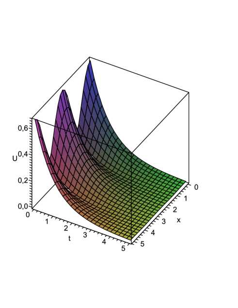
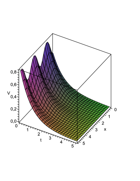
Figure 1: Solution (73) with $k=l=1,\ \lambda^{*}_{11}=2,\ \lambda^{*}_{12}=-1,\ \lambda^{*}_{21}=-2,\ \lambda^{*}_{22}=1,C_{1}=0.2,\ C_{2}=0,\ C_{4}=0.25,\ h=\sqrt{6}.$

Consider the solution listed in case 2 of table 3. Setting $C_{3}=0$, one takes the form

$$\begin{array}[]{l}\varphi(x)=C_{1}\cos(hx)+C_{2}\sin(hx)+C_{4},\\ \psi(x)=\frac{(l+1)\lambda^{*}_{22}}{(k+1)\lambda^{*}_{12}}\Big{(}C_{1}\cos(hx)+C_{2}\sin(hx)\Big{)}-\frac{\lambda^{*}_{11}}{\lambda^{*}_{12}}C_{4},\end{array}$$ (72)

where $h=\sqrt{(k+1)\lambda^{*}_{11}+(l+1)\lambda^{*}_{22}},\ (k+1)\lambda^{*}_{11}+(l+1)\lambda^{*}_{22}>0,\ \lambda^{*}_{11}\lambda^{*}_{22}-\lambda^{*}_{12}\lambda^{*}_{21}=0.$

Using the ansatz (58) and substitution (69), one obtain the three-parameter family of solutions

$$\begin{array}[]{l}U=\Big{(}C_{1}\cos(hx)+C_{2}\sin(hx)+C_{4}\Big{)}^{\frac{1}{k+1}}\exp\Big{(}-\frac{l+1}{l(k+1)}t\Big{)},\\ V=\Big{(}\frac{(l+1)\lambda^{*}_{22}}{(k+1)\lambda^{*}_{12}}\big{(}C_{1}\cos(hx)+C_{2}\sin(hx)\big{)}-\frac{\lambda^{*}_{11}}{\lambda^{*}_{12}}C_{4}\Big{)}^{\frac{1}{l+1}}\exp\Big{(}-\frac{t}{l}\Big{)}.\end{array}$$ (73)

We note that this solution tends to the stable steady-state point $(0,0)$ of system (70) provided $t\rightarrow\infty$ and the restrictions $l>0,\ k>-1$ take place. Moreover, solution (73) is non-negative and satisfies the standard zero-flux conditions on the correctly-specified intervals. For instance, solution (73) with $C_{2}=0$ satisfies the boundary conditions

$$U_{x}|_{x=0}=0,\ V_{x}|_{x=0}=0,\ U_{x}|_{x=j\frac{\pi}{h}}=0,V_{x}|_{x=j\frac{\pi}{h}}=0$$ (74)

on the space interval $[0,j\frac{\pi}{h}],\ j\in\mathbb{N}$ and its components are positive provided $\lambda^{*}_{11}\lambda^{*}_{12}<0,\ C_{4}>\max\{|\frac{(l+1)\lambda^{*}_{22}}{(k+1)\lambda^{*}_{11}}\,C_{1}|,|C_{1}|\}.$ Thus, we established that the exact solutions obtained can satisfy the typical requirements addressed to physically and biologically motivated problems. For example, the solution of the model for the gravity-driven flow of thin films is presented in Fig.1.

4 Discussion

In this paper $Q$-conditional symmetries of the class of RD systems (5) and their application for finding exact solutions are studied. Following the recent paper [16], the notion of $Q$-conditional symmetry of the first type was used for these purposes. The main result is presented in Theorem 1 giving an exhausted list of RD systems of the form (5) with $d^{1}_{u}d^{2}_{v}\neq 0$, which admit such symmetry. It turns out that there are exactly 21 RD systems (up to transformations (38) – (39)) admitting $Q$-conditional symmetry operators of the first type of the form (8) with $\xi^{0}\not=0$. Note that all the operators found are inequivalent to the Lie symmetry operators presented in [8].

It is interesting to compare this result with the known that for the single RD equation

$$U_{t}=\left[D(U)U_{x}\right]_{x}+F(U).$$ (75)

There are several papers devoted to search of $Q$-conditional (non-classical) symmetry operators of equation (75) (see [27, 28] for details). The complete results were derived in [29, 30] for (75) with constant diffusivity and in [31] for (75) with power and exponential diffusivities (note that some operators obtained in [31] are equivalent to the Lie symmetry operators). However, there is no complete description of $Q$-conditional symmetry operators with $\xi^{0}\not=0$ for equation (75) if $D$ and $F$ are arbitrary smooth function. In contrary to the single RD equation, we have done this for the two-component RD systems with arbitrary non-constant diffusivities applying notion of $Q$-conditional symmetry of the first type. It turns out that there are 15 systems of the quite general forms (see cases 1–15 in table 1) admitting such type of symmetry. On the other hand, there is no any single RD equation with the arbitrary function $D$ (or $F$) admitting $Q$-conditional (non-classical) symmetry.

The work is in progress to construct all possible symmetries for the class of RD system (5) with the constant diffusivity ($d^{1}_{u}d^{2}_{v}=0$). The preliminary analysis shows that a wide range new RD systems admitting $Q$-conditional symmetry operators will be found.

Some $Q$-conditional operators obtained were used to construct non-Lie ansätze and to reduce the relevant RD systems to the corresponding ODE systems, which are presented in table 2. Moreover, multiparameter families of exact solutions in the explicit form (66) were constructed for the RD system (67) with an arbitrary diffusivity. Finally, application of the exact solutions for solving the biologically and physically motivated system (70) is presented. It turns out that the relevant boundary value problem at with the zero-flux conditions can be exactly solved on correctly-specified space intervals.

References

• [1]
• [2] Ames WF. Nonlinear Partial Differential Equations in Engineering. New York: Academic Press; 1972.
• [3] Murray JD. Mathematical Biology. Berlin: Springer; 1989.
• [4] Murray JD. Mathematical Biology II: Spatial Models and Biomedical Applications. Berlin: Springer; 2003.
• [5] Okubo A, Levin SA. Diffusion and Ecological Problems. Modern Perspectives, 2-nd ed. Berlin: Springer; 2001.
• [6] Turing AM. The chemical basis of morphogenesis. Phil Trans Roy Soc Lond 1952;237:37-72.
• [7] Feireisl E, Hilhorst D, Mimura M and Weidenfeld R. On a nonlinear diffusion system with resource-consumer interaction. Hiroshima Math J 2003;33:253-95.
• [8] Cherniha R, King JR. Nonlinear Reaction-Diffusion Systems with Variable Diffusivities: Lie Symmetries, Ansätze and Exact Solutions. J Math Anal Appl 2005;308:11-35.
• [9] Zulehner W, Ames WF. Group analysis of a semilinear vector diffusion equation. Nonlinear Anal 1983;7:945-69.
• [10] Cherniha R, King JR. Lie Symmetries of Nonlinear Multidimensional Reaction-Diffusion Systems:I. J Phys A Math Gen 2000;33:267-82, 7839-41.
• [11] Cherniha R, King JR. Lie Symmetries of Nonlinear Multidimensional Reaction-Diffusion Systems:II. J Phys A Math Gen 2003;36:405-25.
• [12] Knyazeva IV, Popov MD. A system of two diffusion equations. CRC Handbook of Lie Group Analysis of Differential Equations, vol. 1. Boca Rato: CRC Press; 1994;171-76.
• [13] Cherniha R, King JR. Lie symmetries and conservation laws of non-linear multidimensional reaction–diffusion systems with variable diffusivities. IMA J Appl Math 2006;71:391-408.
• [14] Nikitin AG. Group classification of systems of non-linear reaction-diffusion equations. Ukrainian Math Bull 2005;2:153-204.
• [15] Cherniha R, Pliukhin O. New conditional symmetries and exact solutions of reaction-diffusion systems with power diffusivities. J Phys A Math Theor 2008;41:185208-22.
• [16] Cherniha R. Conditional symmetries for systems of PDEs: new definition and its application for reaction-diffusion systems. J Phys A Math Theor 2010; 43: 405207-19.
• [17] Cherniha R, Davydovych V. Conditional symmetries and exact solutions of the diffusive Lotka-Volterra system. Math Comput Modelling 2011;54:1238-51.
• [18] Fushchych WI, Shtelen WM, Serov MI. Symmetry analysis and exact solutions of equations of nonlinear mathematical physics. Kluwer; 1993.
• [19] Olver P. Applications of Lie Groups to Differential Equations. Berlin: Springer; 1986.
• [20] Bluman GW, Kumei S. Symmetries and Differential Equations. Berlin:Springer; 1989.
• [21] Bluman GW, Cole JD. The general similarity solution of the heat equation. J Math Mech 1969;18:1025-42.
• [22] Lou S-y. Nonclassical symmetry reductions for the dispersive wave equations in shallow water. J Math Phys 1992;33:4300-5.
• [23] Barannyk T. Symmetry and exact solutions for systems of nonlinear reaction–diffusion equations. Proc Inst Math of NAS of Ukraine 2002;43:80–5.
• [24] Cherniha R, Serov M. Nonlinear Systems of the Burgers-type Equations: Lie and $Q$- conditional Symmetries, Ansätze and Solutions. J Math Anal Appl 2003;282:305-28.
• [25] Murata S. Non-classical symmetry and Riemann invariants. Int J Non-Lin Mech 2006;41:242-46.
• [26] Arrigo DJ, Ekrut DA, Fliss JR, Long Le. Nonclassical symmetries of a class of Burgers’ systems. J Math Anal Appl 2010;371:813-20.
• [27] Cherniha R, Pliukhin O. New conditional symmetries and exact solutions of nonlinear reaction-diffusion-convection equations. J Phys A Math Theor 2007;40:10049-70.
• [28] Kunzinger M, Popovych R.O. Is a nonclassical symmetry a symmetry? In: Proceedings of 4th Workshop ”Group Analysis of Differential Equations and Integrable Systems” 2009; Protaras, Cyprus, p. 107-120.
• [29] Clarkson PA, Mansfield EL. Symmetry reductions and exact solutions of a class of nonlinear heat equations. Physica D 1993;70:250-88.
• [30] Arrigo DJ, Broadbridge P, Hill JM. Nonclassical symmetry reductions of the linear diffusion equation with a nonlinear source. IMA J Appl Math 1994;52:1-24.
• [31] Arrigo DJ, Hill JM. Nonclassical symmetries for nonlinear diffusion and absorption. Stud Appl Math 1995;94:21-39.