Spontaneous Decoherence of Coupled Harmonic Oscillators Confined in A Ring

Abstract

We study the spontaneous decoherence of the coupled harmonic oscillators confined in a ring container, where the nearest-neighbor harmonic potentials are taken into consideration. Without any external symmetry breaking field or surrounding environment, the quantum superposition state prepared in the relative degrees of freedom gradually loses its quantum coherence spontaneously. This spontaneous decoherence is interpreted by the hidden couplings between the center-of-mass and relative degrees of freedoms, which actually originates from the symmetries of the ring geometry and corresponding nontrivial boundary conditions. Especially, such spontaneous decoherence completely vanishes at the thermodynamical limit because the nontrivial boundary conditions become trivial Born-von Karman boundary conditions when the perimeter of the ring container tends to infinity. Our investigation shows that a thermal macroscopic object with certain symmetries has chance to degrade its quantum properties even without applying an external symmetry breaking field or surrounding environment.

I INTRODUCTION

Quantum decoherence has been a subject of active research since the quantum mechanics was established Zurek91 . The revival of the studies of the decoherence as a hot subject merits from the development of the science and technology of the quantum information. As the physical states in quantum mechanics are described by the superposition of some eigenstates, the coherence existing between different eigenstates is the important criteria for that whether the quantum properties of the system remain or not. In this sense, the quantum decoherence explains the emergence of the classical limit of a system with quantum nature, which apparently determines the quantum-classical boundary Haroche98 ; Zurek03 ; Bennett00 ; Quan06a .

In the first place, quantum decoherence was named for the collapse of the wave function in the Copenhagan interpretation Howard04 . In stead of generating actual wave function collapse, it only gives the appearance of the wave function collapse. Nowadays, the studies of the decoherence focus on the quantum correlation between the system and its environment Joos85 ; Zeh70 ; Zurek81 ; Zhou02 . As commonly understood, the decoherence process can be viewed as that the quantum system loses information into its environment. Mathematically, losing information in decoherence process can be defined by the disappearance of the off-diagonal elements of the system’s reduced density matrix. A perfect decoherence process requires that the environment approaches its thermodynamic limit, whose infinite degrees of freedom guarantee the infinitely long recurrence time of the decoherence process Sun93 ; Zurek94 ; Sun01 ; Zeh01 ; Joos03 ; Schlosshauer05 ; Xue06 .

To reveal the mechanism of the quantum decoherence, Heisenberg introduced a random phase factor according to the uncertainty principle. This phase factor also results in the randomness of the coefficients of the off-diagonal elements of the system’s reduced density matrix, whose average on time tends to zero eventually. However, the uncertainty principle is not the only mechanism to cause decoherence, which has been verified experimentally Durr98 ; Arndt99 . Generally speaking, the random factor originally comes from the interaction between the quantum system and its environment. In contrast of the external environment mentioned above, we are more interested in an internal one Ommes94 ; Zhang02 . For the most quantum systems, only some subspaces of the complete Hilbert space of the system are concentrated on, whose adjoint space can be regarded as the “internal” environment with interaction between these two spaces such as the spin-orbit interaction, the electron-phonon interaction and so on. Instead of infinite degrees of freedom the external environment has, the internal environment only possesses a few degrees of freedom.

Previous theoretical research indicated that due to the spontaneous symmetry breaking Wezel05 ; Wezel06 ; Wezel08a ; Wezel08b in association with quantum phase transition Quan06b , the quantum decoherence emerges in the multi-particle system when a small but finite symmetry breaking field was added to a closed symmetric quantum system. Such decoherence is called “intrinsic decoherence” because there is no usual environment at all. When the symmetry is broken, a serious of thin spectrum emerge in the vicinity of the original energy levels. The subtle energy differences of the thin spectrum actually results in the spontaneous decoherence. Recently, researchers show than the spontaneous decoherence also can be induced by gravitational time dilation Pikovski15a ; Pikovski15b ; Gooding15 .

In this paper, we shall study the spontaneous decoherence of closed multi-particle system without symmetry breaking. Considering $N$ coupled harmonic oscillators confined in a ring container, the Hamiltonian can be decoupled into one center-of-mass motion and $N-1$ relative motions. It is essential that the harmonic potentials between oscillators are periodically repeated because of the ring configuration. Such bosonic multi-particle system possesses $U(1)\otimes C_{\mathrm{N}}$ symmetry, where the continuous $U(1)$ symmetry and discrete $C_{\mathrm{N}}$ symmetry respectively relate the center-of-mass and relative motions’ symmetries. Then nontrivial boundary conditions emerge in order to guarantee the single-valuedness of the wave function, which eventually results in that the total energy spectrum not only depends on the excitations of the relative motion, but also on the total momentum corresponding to the center-of-mass motion. Similar to Aharonov-Bohm effect, the nontrivial boundary conditions actually are equivalent to applying an induced gauge fields Yang61 . This hidden coupling between the center-of-mass motion and relative motions introduces a series of thin spectrum of the total momentum, which contributes to the decoherence process of relative motions. If the center-of-mass motion is not condensed to the state with single momentum, the spontaneous decoherence process occurs in the superposition states in the relative motions. Since there is no environment or symmetry breaking field at all, the decoherence in our model is definitely intrinsic and its dynamical process is spontaneous. The paradox of such spontaneous decoherence is the information represented by the quantum coherence is mysteriously missing in a completely closed system. The key point to explain this is that the center-of-mass motion actually acting like a surrounding environment to the relative motions we concentrate on. The information is only transferred from the subspace of the complete Hilbert space into its adjoint space.

This article is arranged as follows. We describe the multi-particle model and derive the nontrivial boundary conditions in Sec. II. Then the explicit total energy spectrum including all the thin spectrum is obtained in Sec. III. In Sec. IV, we demonstrate how the thin spectrum contributes to the dynamic decoherence process. We conclude in Sec V.

II COUPLED HARMONIC OSCILLATORS CONFINED IN A RING CONTAINER

II.1 Model setup

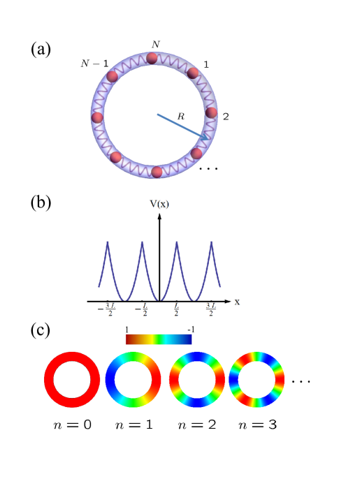
Figure 1: (Color online) (a) Schematic illustration of the coupled harmonic oscillators confined in a ring container. Here, the light blue torus and the red spheres represent the ring container with the perimeter $R$ and the oscillators, respectively. (b) Schematic illustration of the periodic harmonic potential. Here, $x$ denotes any displacement difference between nearest neighbor oscillators. (c) Schematic illustration of the real part of the center-of-mass motion wavefunction versus the displacement $X_{0}$ for the first four quantum number $n$.

To investigate the mechanism of the decoherence due to symmetries of system, we consider a bosonic multi-particle system confined in a ring container (Fig. 1(a)), which is modeled as $N$ coupled harmonic oscillators with Hamiltonian

$$\hat{H}=\sum_{j=1}^{N}\left[\frac{\hat{p}_{j}^{2}}{2m}+V(\hat{x}_{j}-\hat{x}_{j+1})\right],$$ (1)

where

$$V(\hat{x}_{j}-\hat{x}_{j+1})=\frac{\kappa}{2}\left(\hat{x}_{j}-\hat{x}_{j+1}\right)^{2}$$ (2)

are harmonic potentials between nearest neighbor oscillators. Here, $\hat{p}_{j}$ and $\hat{x}_{j}$ are the momentum and the displacement of the $j-$th oscillator. For the sake of simplicity, the oscillator mass $m$ and the spring constant $\kappa$ are supposed to be identical for all oscillators, and the system is considered as one-dimensional since the cross section radius of the ring container is much smaller than the radius of the ring $R$. If all the oscillators only vibrate in the vicinity of their equilibrium positions, it is the textbook example of the phonons in the solid state physics with Born-von Karman boundary condition. However, in the present situation, the oscillators can potentially amove far away from their equilibrium positions if their kinetic energies are sufficiently large. In this case, the harmonic potentials becomes periodic as

$$V(x_{j}-x_{j+1}+nL)=V(x_{j}-x_{j+1})$$ (3)

when any of the displacement difference between the nearest neighbor oscillators is augmented by $nL$ ($n$ is an integer). This periodic potential is schematically plotted in Fig. 1(b). Here, $L=2\pi R$ is the perimeter of the ring container. Since the harmonic potentials only involve the displacement difference between the nearest neighbor oscillators, the above coupled-oscillator system can be decoupled to $N$ oscillators, which correspond to one center-of-mass motion and $(N-1)$ relative motions.

To decouple the system into $N$ oscillators, we successively perform the Fourier transformation as $\left(\hat{q}_{j}=\hat{p}_{j},\hat{x}_{j}\right)$

$$\hat{Q}_{k}=\begin{cases}\sqrt{\frac{2}{N}}\sum_{j=1}^{N}\hat{q}_{j}\cos\left(\frac{2\pi kj}{N}\right),&1\leq k\leq\frac{N}{2},\\ \sqrt{\frac{2}{N}}\sum_{j=1}^{N}\hat{q}_{j}\sin\left(\frac{2\pi kj}{N}\right),&k>\frac{N}{2},\end{cases}$$ (4)

where $\hat{Q}_{k}=\hat{P}_{k},\hat{X}_{k}$ $(k=1,\cdots,N-1)$ are the momentums and the displacements of the $N-1$ independent relative motions. Besides the relative motions, there is unique center-of-mass motion, whose momentum and displacement are described as $\hat{P}_{0}=\sum_{j=1}^{N}\hat{p}_{j}$ and $\hat{X}_{0}=1/N\sum_{j=1}^{N}\hat{x}_{j}.$ We introduce the different forms for momentums and the displacements when $1\leq k\leq N/2$ and $k>N/2$ in order to guarantee that they are still Hermitian operators and satisfy the standard commutaion relation $\left[\hat{X}_{k},\hat{P}_{k^{\prime}}\right]=i\hbar\delta_{k,k^{\prime}}$. After the Fourier transformation, the Hamiltonian becomes $N$ decoupled harmonic oscillators as

$$\hat{H} = \hat{H}_{0}+\sum_{k=1}^{N-1}\hat{H}_{k}\text{,}$$ (5a)

$$\hat{H}_{k} = \frac{\hat{P}_{k}^{2}}{2m}+\frac{\kappa}{2}\left(2\sin\frac{\pi k}{N}\right)^{2}\hat{X}_{k}^{2}.$$ (5b)

It should be indicated that the zero-th Hamiltonian

$$\hat{H_{0}}=\frac{\hat{P}_{0}^{2}}{4mN}=\frac{1}{2mN}\left(\sum_{j=1}^{N}\hat{p}_{j}\right)^{2}$$ (6)

describes the center-of-mass motion of the multiple particle system, which is regarded as a whole carrying a kinetic energy associated with total mass of the system. The rest part of the Hamiltonian $\hat{H}_{R}=\hat{H}-\hat{H}_{0}=\sum_{k=1}^{N-1}\hat{H}_{k}$ describes the decoupled $N-1$ relative motions. Obviously, each relative mode is described by a periodic harmonic oscillator. Although the periodicities of these relative motions are no longer simply demonstrated, the sum of all relative harmonic oscillators potentials still possesses the periodicities shown in Eq. (3). By solving the eigenvalue problem of the system, we can obtain the thin spectrum which plays essential role in our spontaneous quantum decoherence process.

II.2 Origin of the thin spectrum

Although the center-of-mass motion and relative motions seems independent with each other in the Hamiltonian, there is a hidden coupling between them due to the symmetry of the system. For a given quantum system, the energy spectrum and eigen-wavefunctions are not only governed by its Hamiltonian, but also determined by the boundary conditions which depend on the symmetries of the system Yang61 . We will find the boundary conditions for our system as follows.

We first analyse the existing symmetries of the system shown in Fig.1(a). If all the oscillator displacements $x_{j}(j=1,\ldots,N)$ are augmented by the same increment $\delta x$, Hamiltonian keeps unchanged, which means the system possesses $U(1)$ symmetry. Since the Hamiltonian has been decoupled as Eq. (5a), the eigenstate of the system is obtained as

$$\Psi\left(\mathbf{X}\right)=\exp\left(\frac{i}{\hbar}P_{0}X_{0}\right)\chi\left(\mathbf{X}\right),$$ (7)

where the plane wave $\exp\left(iP_{0}X_{0}/\hbar\right)$ and the product state

$$\chi\left(\mathbf{\mathbf{X}}\right)=\prod\limits_{j=1}^{N-1}\chi_{j}\left(X_{j}\right)$$ (8)

describes the center-of-mass motion and the relative motions, respectively. Here, the vector $\mathbf{X}=\{X_{1},X_{2},\ldots,X_{N-1}\}$ represents the displacements of relative motions as well as $\mathbf{x}=\{x_{1},x_{2},\ldots,x_{N-1}\}$ is the displacements of original oscillators. They are linked by the a linear transformation as $\mathbf{X}=M\mathbf{x}$, where the transformation matrix is determined by Eq. (4). If all the oscillator displacements $x_{j}(j=1,\ldots,N)$ are augmented by the same increment $\mu L$ ($\mu$ is integer), the relative motions keep unchanged because all the relative displacements are unchanged, but there is an additional phase to the center-of-mass motion wave function

$$\Psi^{\prime}\left(\mathbf{\mathbf{X}}\right)=\exp\left(\frac{i}{\hbar}P_{0}\left(X_{0}+\mu L\right)\right)\chi\left(\mathbf{X}\right).$$ (9)

The single-valuedness condition of the quantum mechanics requires $\Psi^{\prime}\left(\mathbf{\mathbf{X}}\right)=\Psi\left(\mathbf{X}\right),$ which leads to the quantized total momentum as ($n$ is integer)

$$P_{0}\left(n\right)=n\frac{\hbar}{R}.$$ (10)

The real part of the plane waves of the center-of-mass motion versus the displacement $X_{0}$ is depicted in Fig. 1(c). With the quantum number $n$ increases, the nodes number of the real part of the center-of-mass motion wavefunction also increases.

Besides this continuous symmetry, there is discrete symmetry due to the periodicity of the harmonic potential shown in Eq. (3). When any one of the displacement $x_{j}$ is augmented by $\mu L$, the Hamiltonian is still unchanged. In this sense, the operation not only introduces a similar phase to the center-of-mass motion as

$$\Psi^{\prime}\left(\mathbf{\mathbf{\mathbf{X}}^{\prime}}\right)=\exp\left[\frac{i}{\hbar}P_{0}\left(n\right)\left(X_{0}+\frac{1}{N}\mu L\right)\right]\chi\left(\mathbf{\mathbf{X}}^{\prime}\right),$$ (11)

but also change the displacements of the relative motions to $\mathbf{\mathbf{X}}^{\prime}=\mathbf{X}+\mu L\boldsymbol{M}_{j_{0}}.$ Here, $\boldsymbol{M}_{j_{0}}$ is the column vector of the transformation matrix $\mathbf{M}$. If we only focus on the additional phase of the center-of-mass motion and substitute the quantized total momentum in Eq. (10), the phase $\exp\left(i2\pi n\mu/N\right)$ actually only have $N$ possible values for $\mod[n\mu,N]=0,1,\ldots,N-1,$ where $\mod[x,y]$ gives the remainder on division of x by y. These $N$ operations actually constitutes the $N$ elements of the $C_{N}$ group. Therefore, the total system symmetry group is $U(1)\otimes C_{\mathrm{N}}$.

To obtain the energy spectrum, the corresponding Schrodinger equation is taken into consideration as

$$\hat{H}\Psi\left(\mathbf{X}\right)=E\left(n\right)\Psi\left(\mathbf{X}\right),$$ (12)

where the eigen-energy contains the kinetic energy of center-of-mass motion and the energies of the relative motions as

$$E\left(n,\alpha\right)=\frac{n^{2}\hbar^{2}}{2mNR^{2}}+\epsilon\left(\alpha\right).$$ (13)

Here, we already have substituted the quantized total momentum into the kinetic energy $P_{0}^{2}/2mN$. Since the total momentum commutes with all displacements of relative motions as $\left[\hat{X}_{k},\hat{P}_{0}\right]=i\hbar\delta_{k,0}$, the eigenstates describing the relative motions also satisfy the following Schrodinger equation as

$$\hat{H}\chi\left(\mathbf{\mathbf{X}}\right)=\epsilon\chi\left(\mathbf{X}\right).$$ (14)

Usually, the energy spectrum of the relative modes $\epsilon$ is independent of the total momentum $P_{0}$ and the coherence of the relative motion states can be maintained all the time. However, single-valuedness condition requires the wavefunction in Eq. (11) is the same as the wavefunction in Eq. (7), which leads to

$$\chi\left(\mathbf{X}\right)=\exp\left(i\mu\theta_{n}\right)\chi\left(\mathbf{X}+\mu L\boldsymbol{M}_{k_{0}}\right)$$ (15)

with $\theta_{n}=2\pi n/N$ for any $k_{0}=1,2,\ldots,N-1$. Here, the boundary conditions in Eq. (15) actually can guarantee the single-valuedness condition for any $\mu$ as

$$\chi\left(\mathbf{\mathbf{X}}\right) =\exp\left(i\theta_{n}\right)\chi\left(\mathbf{X}+L\boldsymbol{M}_{k_{0}}\right)$$

$$=\exp\left(i2\theta_{n}\right)\chi\left(\mathbf{X}+2L\boldsymbol{M}_{k_{0}}\right)$$

$$=\ldots=\exp\left(i\mu\theta_{n}\right)\chi\left(\mathbf{X}+\mu L\boldsymbol{M}_{k_{0}}\right).$$ (16)

Obviously, $\theta_{n}$ depends on the total momentum $P_{0}$, which eventually results in that the energy of relative motions $\epsilon\left(n,\alpha\right)$ becomes dependent of the total momentum. For different quantum number $n$ of the total momentum, the group of the energy levels form the thin spectrum, which plays the essential role in the spontaneous decoherence. The Hamiltonian in the first place possesses the $C_{N}$ symmetry implying periodic $\theta_{n}$ as $\theta_{n}$=$\theta_{n+\mu N}$, therefore the thin spectrum is also periodic as $\epsilon\left(n,\alpha\right)=\epsilon\left(n+\mu N,\alpha\right).$ Since the Hamiltonian has inversion symmetry when $\mathbf{x}\rightarrow-\mathbf{x},$ which imply that the thin spectrum is even function of $n$ as $\epsilon\left(n,\alpha\right)=\epsilon\left(-n,\alpha\right).$

We will solve the energy spectrum of the relative motions from its eigen-equation in Eq. (14) together with the nontrivial boundary conditions in Eq. (15) in order to obtain the thin spectrum depending on the quantum number $n$ of the total momentum in the next section.

III THE TOTAL ENERGY SPECTRUM

Since the harmonic oscillator potential for relative motions are still periodic, according to the Floquet theorem Magnus04 , the $k-$th relative motion can be rewritten as

$$\chi_{k}\left(X_{k}\right) = e^{iq_{k}X_{k}}u_{k}\left(X_{k}\right)$$ (17)

with wave vector $q_{k}$ and the periodic part $u_{k}\left(X_{k}\right).$ According to Eq. (8), the total relative motions are described by the product state as

$$\chi\left(\mathbf{\mathbf{X}}\right)=e^{\sum_{k=1}^{N-1}iq_{k}X_{k}}\prod\limits_{k=1}^{N-1}u_{k}\left(X_{k}\right).$$ (18)

In order to satisfy the boundary conditions as Eq. (15), we calculate the wavefunction of all the relative motions when the $j_{0}-$th oscillator displacement is augmented by $L$ as

$$\chi\left(\mathbf{X}+L\boldsymbol{M}_{j_{0}}\right)$$ (19)

$$= e^{\sum_{k=1}^{N-1}iq_{k}\left(X_{k}+LM_{k_{0}}^{k}\right)}\prod\limits_{k=1}^{N-1}u_{k}\left(X_{k}+LM_{k_{0}}^{k}\right)$$

$$= e^{\sum_{k=1}^{N-1}iq_{k}LM_{k_{0}}^{k}}e^{\sum_{k=1}^{N-1}iq_{k}X_{k}}\prod\limits_{k=1}^{N-1}u_{k}\left(X_{k}+LM_{k_{0}}^{k}\right)$$

$$= e^{\sum_{k=1}^{N-1}iq_{k}LM_{k_{0}}^{k}}\chi\left(\mathbf{X}\right),$$

where $M_{k_{0}}^{k}$ are the elements of the vector $\boldsymbol{M}_{k_{0}}=\left(M_{k_{0}}^{1},M_{k_{0}}^{2},\ldots,M_{k_{0}}^{N-1}\right)$ and in the last step we apply the periodicity of the wavefunctions $\left\{u_{k}\left(X_{k}\right)\right\}$ as

$$\prod\limits_{k=1}^{N-1}u_{k}\left(X_{k}+LM_{k_{0}}^{k}\right)=\prod\limits_{k=1}^{N-1}u_{k}\left(X_{k}\right).$$ (20)

In contrat with the boundary conditions in Eq. (15), we actually obtain the constrains for the wave vectors $\{q_{k}\}$ as

$$LM_{k_{0}}^{k}q_{k}+\theta_{n}=0,$$ (21)

which should be satisfied for any $k_{0}.$ The $N-1$ constrains completely determine the wave vectors $\{q_{k}\}$. In the vector form, it can be rewritten as

$$L\mathbf{M}\mathbf{q}+\theta_{n}\mathbf{I}=0,$$ (22)

where $\mathbf{q}=(q_{1},q_{2,}\ldots,q_{N-1})^{T}$ and $\mathbf{I}=(1,1,\ldots,1)^{T}$. The solution is straightforwardly obtained as (see Appendix A)

$$q_{j}=\begin{cases}q,&1\leq k\leq\frac{N-1}{2},\\ 0,&\frac{N+1}{2}\leq k\leq N-1,\end{cases}$$ (23)

for odd number $N$ and

$$q_{j}=\begin{cases}q,&1\leq k\leq\frac{N}{2}-1,\\ \frac{q}{2},&k=\frac{N}{2},\\ 0,&\frac{N}{2}+1\leq k\leq N-1,\end{cases}$$ (24)

for even number $N$ with $q=\frac{\sqrt{2}n}{\sqrt{N}R}.$ It indicates that for those relative motions with $k<N/2$ the wave vectors $q$ are exactly same, which is proportional to the quantum number $n$ as well as the total momentum $P_{0}\left(n\right).$ While for those relative motions with $k>N/2$ the wave vectors vanish. In this sense, the phase factor $\theta_{n}$ resulting from the total momentum now is divided into individual phase factors of those relative motions with $k\leq N/2$. Actually, the consequence of the nontrivial boundary conditions is adding an additional phase factor in Eq. (15), which actually is equivalent to introducing a gauge field onto the relative motions (see Appendix B).

Therefore it is feasible to deal with single relative motion in order to obtain the corresponding energy spectrum once the individual periodicity of the relative motion is determined. When the $j_{0}$-th oscillator’s displacement is augmented by $\mu L$, the change of the relative motion displacements is $\mathbf{\mathbf{X}}^{\prime}=\mathbf{X}+\mu L\boldsymbol{M}_{k_{0}}$ and the periodic part of the wavefunction $u_{k}\left(X_{k}\right)$ satisfies

$$u_{k}\left(X_{k}\right) = u_{k}\left(X_{k}+LM_{k_{0}}^{k}\right).$$ (25)

Since we can permutate the indices of the original oscillators such as $\{k_{0},k_{0}+1,\ldots,N,1,2,\ldots,k_{0}-1\}\rightarrow\{1,2,\ldots,N\}$ in order to always augment the first oscillator’s displacement, the periodicities of those relative motions are considered as $u_{k}\left(X_{k}\right)=u_{k}\left(X_{k}+LM_{1}^{k}\right).$ In this sense, we can solve the Schrodinger equation

$$\hat{H_{k}}\chi_{k}\left(X_{k}\right)=\epsilon_{k}\chi_{k}\left(X_{k}\right)$$ (26)

and corresponding boundary conditions, which require both the wavefunction and derivative of the wavefunction is continuous as

$$\chi_{k}\left(-\frac{L}{2}M_{1}^{k}\right) = e^{iq_{k}LM_{1}^{k}}\chi_{k}\left(\frac{L}{2}M_{1}^{k}\right),$$ (27a)

$$\left.\frac{d}{dX_{k}}\chi_{k}\left(X_{k}\right)\right|_{X_{k}=-\frac{L}{2}M_{1}^{k}} = e^{iq_{k}LM_{1}^{k}}\left.\frac{d}{dX_{k}}\chi_{k}\left(X_{k}\right)\right|_{X_{k}=\frac{L}{2}M_{1}^{k}}.$$ (27b)

The energy spectrum depends on quantum number $n$ can be approximately obtained as (see Appendix C)

$$\epsilon_{k}\left(n,\alpha\right)=\left(\frac{1}{2}+\alpha+\delta_{k}\left(n,\alpha\right)\right)\hbar\omega_{k}$$ (28)

with the frequency of the oscillator of the $k$-th relative motion $\omega_{k}=4\sqrt{\kappa/m}\sin\left(\pi k/N\right)$. The explicit form of the total-momentum dependent term $\delta_{k}\left(n,\alpha\right)$ can be found in Appendix C.

The total thin spectrum is the sum of all the energies of the relative motions as $\epsilon\left(n,\alpha\right)=\sum_{k=1}^{N-1}\epsilon_{k}\left(n,\alpha\right).$ The schematics of the the spectrum is depicted in Fig.2, which is almost quadratic of the $n$ and linear of $\alpha$. The subtle difference between different thin spectra with different excitation quantum number of the relative modes $\alpha$ usually still depends on the total momentums, which leads to the decoherence of the relative modes. The details of such decoherence process will be discussed in the next section.

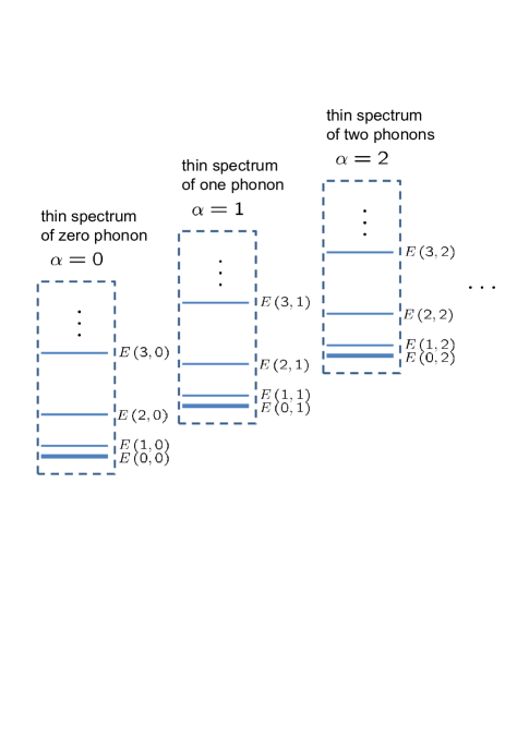
Figure 2: Schematic illustration of the total energy spectrum $E\left(n,\alpha\right)$. The thin spectrum is almost quadratic of the quantum number $n$ of the total momentum, and linear of the quantum number $\alpha$ of the relative motions.

IV DECOHERENCE OF THE RELATIVE MOTIONS

IV.1 Decoherence factor

To explore the decoherence of the relative modes caused by the thin spectrum, we consider the dynamics of an actual qubit of the multi-particle system. The qubit is chosen as $(a\left|0\right\rangle+b\left|1\right\rangle)\otimes\left|n\right\rangle$with the ground state of the relative modes $\left|\alpha=0\right\rangle$, the first excitation state of the relative modes $\left|\alpha=1\right\rangle$ and the center-of-mass state $\left|n\right\rangle$ (see fig.2). If the multi-particle system condensates on the BEC state with a single momentum, which is equivalent to that $\left|n\right\rangle$ only contains a single mode plane wave, the effect of the thin spectrum is adding a phase factor to the off-diagonal elements of the reduced density matrix of the relative modes and thus no decoherence process occurs. However, in a relative high temperature such as $k_{B}T\gg\hbar^{2}/2mNR^{2},$ the center-of-mass state usually stays in thermal state as

$$\rho_{T}=\frac{1}{Z}\sum_{n=-\infty}^{\infty}e^{-\beta E\left(n,\alpha\right)}\left|n\right\rangle\left\langle n\right|$$ (29)

for a macroscopic object with $\beta^{-1}=k_{B}T$, where the thin spectrum is labeled by the quantum number $n$ of total momentum and $\alpha$ of the relative motions as

$$E\left(n,\alpha\right) = \frac{n^{2}\hbar^{2}}{2mNR^{2}}+\epsilon\left(n,\alpha\right)$$ (30)

and $Z=\sum_{n}e^{-\beta E\left(n,0\right)}$ is the partition function corresponding to the product of the center-of-mass thermal state and the ground state of the relative modes.

We prepare the initial state of the qubit on its ground state $\left|0\right\rangle$ and then apply a rotation to transform the ground state into $a\left|0\right\rangle+b\left|1\right\rangle.$ In this case, the initial density matrix is the product of the thermal state density matrix and qubit one as

$$\rho_{0} = \rho_{T}\otimes\rho_{Q}$$ (31)

$$= \frac{1}{Z}\sum_{n=-\infty}^{\infty}e^{-\beta E\left(n,0\right)}\left|n\right\rangle\left\langle n\right|\times$$

$$(a\left|0\right\rangle+b\left|1\right\rangle)(a^{*}\left\langle 0\right|+b^{*}\left\langle 1\right|).$$

Since we have solved the total energy spectrum of the system, the time evolution of the eigenstate $\left|n,\alpha\right\rangle\equiv\left|n\right\rangle\otimes\left|\alpha\right\rangle(\alpha=0,1)$ can be described by a time evolution operator as

$$U_{t}\left|n,\alpha\right\rangle=\exp\left[-\frac{i}{\hbar}E\left(n,\alpha\right)t\right]\left|n,\alpha\right\rangle.$$ (32)

Then the time evolution of the density matrix is

$$\rho_{t} = U_{t}\rho_{0}U_{t}^{\dagger}$$ (33)

$$= \frac{1}{Z}\sum_{n=-\infty}^{\infty}e^{-\beta E\left(n,0\right)}\left|n\right\rangle\left\langle n\right|\left(\left|a\right|^{2}\left|0\right\rangle\left\langle 0\right|+\left|b\right|^{2}\left|1\right\rangle\left\langle 1\right|\right.$$

$$\left.+a^{*}be^{-\frac{i}{\hbar}(E\left(n,1\right)-E\left(n,0\right))t}\left|1\right\rangle\left\langle 0\right|+h.c.\right).$$

Tracing out the degree of freedom of the center-of-mass, we can define the decoherence factor from the coefficients of the off-diagonal elements as

$$F=\left|\frac{1}{Z}\sum_{n=-\infty}^{\infty}e^{-\beta E\left(n,0\right)}e^{-\frac{i}{\hbar}\Delta E\left(n\right)t}\right|$$ (34)

with $\Delta E\left(n\right)=E\left(n,1\right)-E\left(n,0\right)$. Obviously, the decoherence factor is equal or less then $1$, which characterizes the completeness of the decoherence process. $F=1$ means the state has the same coherence as the initial quantum state, $F<1$ means the decoherence occurs and the multi-particle system becomes classical when $F=0.$

IV.2 Time scale of the decoherence at two limits

Since the ground state is the product of the ground states of all relative motions, namely $\left|0\right\rangle=\prod_{k=1}^{N-1}\otimes\left|0_{k}\right\rangle$, the ground state energy

$$E\left(n,0\right)=\frac{n^{2}\hbar^{2}}{2mNR^{2}}+\sum_{k=1}^{N-1}\left(\frac{1}{2}+\delta_{k}^{n}\right)\hbar\omega_{k}$$ (35)

is the summation of the ground state energy of all relative motions and the kinetic energy of center-of-mass motion. Additionally, since the first excited state is the state that $\left(N-1\right)$-th relative motions remain at ground state and only the first relative motion is excited to the excited state as $\left|1\right\rangle=\left|1_{1}\right\rangle\prod_{k=2}^{N-1}\otimes\left|0_{k}\right\rangle,$ the energy difference in the decoherence factor actually only depends on the energy level spacing of the ground state and the excited state of the first relative motion, namely

$$\Delta E\left(n\right)=\epsilon_{1}\left(n,1\right)-\epsilon_{1}\left(n,0\right)$$

$$\approx-\hbar\omega_{1}\frac{g}{2}\cos\left(4\pi\frac{n}{N}\right),$$ (36)

where $g\hbar\omega_{1}=\Delta E\left(N/4\right)-\Delta E\left(0\right)$ is the maximum energy difference between thin spectrum. Here, we have assumed the thin spectrum has the cosine type oscillating behavior because it is periodic even function associating with the period $N/2$ of phase factor $\theta_{n}$. Under this approximation, the decoherence factor in Eq. (34) can be written in a series of Bessel functions as

$$F \approx\left|\frac{1}{Z}\int_{-\infty}^{\infty}e^{-\beta\Delta_{e}^{\prime}n^{2}}e^{i\frac{g}{2}\omega_{1}t\cos\left(4\pi\frac{n}{N}\right)}dn\right|$$

$$=\left|\frac{1}{Z}\int_{-\infty}^{\infty}e^{-\beta\Delta_{e}^{\prime}n^{2}}\sum_{\gamma=-\infty}^{\infty}e^{i\alpha\left(4\pi\frac{n}{N}+\frac{\pi}{2}\right)}J_{\gamma}\left[\frac{g}{2}\omega_{1}t\right]dn\right|$$

$$=\left|\sum_{\gamma=-\infty}^{\infty}J_{\gamma}\left(\frac{g}{2}\omega_{1}t\right)e^{i\gamma\frac{\pi}{2}}\exp\left(-\frac{4\pi^{2}\gamma^{2}}{N^{2}\beta\Delta_{e}^{\prime}}\right)\right|.$$ (37)

Here, we have assumed the second term in $E\left(n,0\right)$ is quadratic of $n$ as $\sum_{k=1}^{N-1}\delta_{k}^{n}\hbar\omega_{k}=\Delta_{e}n^{2}$ and $\Delta_{e}^{\prime}=\Delta_{e}+\hbar^{2}/2mNR^{2}.$ We also have neglected the $n$ independent term because they will vanish in the absolute value of the Eq. (34).

Obviously for the first limit, if $4\pi^{2}/N^{2}\beta\Delta_{e}^{\prime}\gg 1$ the last term exponentially decays as $\gamma$ increases and eventually only $\gamma=0$ term contributes to the decoherecne factor as $F=J_{0}\left(\frac{g}{2}\omega_{1}t\right).$ In this limit, the decoherence factor is independent of the temperature and has an oscillating behavior associating with the $0$-th Bessel function.

We can obtain the decoherence factor in another limit. Since the decoherence factor in Eq.(34) basically is the integral of both the Gaussian part and the dynamic phase, if the period of the dynamic phase ($N/2$) is greater than the full width at half maximum (FWHM) of the Gaussian part, only the first period of the thin spectrum contributes to the decoherence factor. In this sense, the energy difference is approximately linear one as

$$\Delta E\left(n\right)= \epsilon_{1}\left(n,1\right)-\epsilon_{1}\left(n,0\right)$$

$$\approx \frac{\Delta_{g}}{N}\left|n\right|\hbar\omega_{k}$$ (38)

with $\Delta g=g_{1}\left(1,1\right)-g_{1}\left(1,0\right)$. The defininition of function $g_{1}\left(k,m\right)$ can be found in Appendix C. The decoherence factor actually possesses an exponentially decay behavior as

$$F \approx\left|\frac{1}{Z}\int_{-\infty}^{\infty}e^{-\beta\Delta_{e}^{\prime}n^{2}}e^{-i\sqrt{\frac{\kappa}{m}}2\pi\frac{\Delta_{g}}{N^{2}}\left|n\right|t}dn\right|$$

$$=e^{-\left(\frac{t}{\tau}\right)^{2}}\sqrt{1+\mathrm{Erfi}\left(\frac{t}{\text{$\tau$}}\right)^{2}},$$ (39)

where

$$\tau=\sqrt{\frac{\beta N^{4}m\Delta_{e}^{\prime}}{\pi^{2}\Delta_{g}^{2}\kappa}},$$ (40)

$\mathrm{Erfi}(t/\tau)$ is the imaginary error function and the summation becomes a integral at high temperature such as $k_{B}T\gg\hbar^{2}/2mNR^{2}$. The typical time scale of the decoherence is

$$\tau_{spon}=\sqrt{\frac{2\left(\pi-2\right)}{\pi}}\tau\approx 0.85\tau.$$ (41)

Since usually the $\Delta_{e}$ and $\Delta_{g}$ usually depend on all other parameters such as $N$,$T$, $\kappa,$ $m$ and $R$ (see Appendix C), it is hard to determine the exact dependence of the decoherence factor on those parameters, and we will present numerical analysis in the next subsection. Especially, if the lattice constant $R/N$ is unchanged while increasing the ring container radius $R$, the decoherence tends to infinity, $\Delta_{e}$ and $\Delta_{g}$ both tend to constant and thus the $\tau_{spon}$ is proportional to the $\sqrt{R}$. This implies no spontaneous decoherence occurs in the thermodynamical limit. This is consistent with the textbook example of phonon in the solid state physics.

IV.3 Numerical results

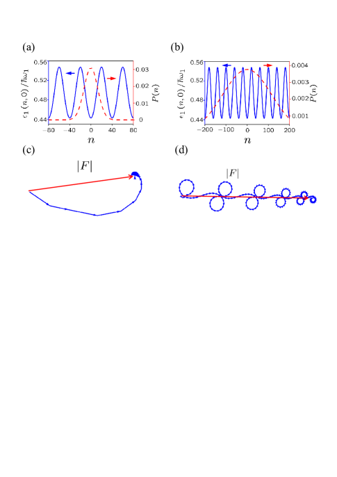
Figure 3: (a) (b) The typical thin spectrum $\epsilon_{1}\left(n,0\right)$ for the zero phonon of the first relative motion and the normalized Gaussian part $P\left(n\right)$ versus the quantum number $n$. The blue solid line and the red dashed line represent $\epsilon_{1}\left(n,0\right)$ and $P\left(n\right)$, respectively. The parameters are chosen as $N=80,R=0.5\mu m,\kappa=10^{-13}N/s,m=40m_{p}$ with $m_{p}$ is mass of proton. The temperature is $T=0.1\mu K$ for (a) and $T=8\mu K$ for (b). (c) and (d) are the typical vector summation pictures of the decoherence factor $\left|F\right|$ respectively corresponds to the cases (a) and (b). The red arrow and the blue arrows respectively represent the decoherence factor $\left|F\right|$ and the successive terms in decoherence factor. Obviously, for case (a) there is only the single period of the thin spectrum contributing to the decoherence factor. While for the case (b) there are multi-periods of the thin spectrum contributing to the decoherence factor.

The numerical calculations based on Eq. ( 34) are present in this section. The typical thin spectrum $\epsilon_{1}\left(n,0\right)$ for the zero phonon of the first relative motion and the normalized Gaussian part

$$P\left(n\right)=\frac{1}{Z}e^{-\beta\left(\frac{n^{2}\hbar^{2}}{2mNR^{2}}\right)}$$ (42)

in the decoherence factor versus the quantum number $n$ are depicted in Fig. 3(a) and (b). The parameters are chosen as $N=80,R=0.5\mu m,\kappa=10^{-13}N/s,m=40m_{p}$ with $m_{p}$ the mass of proton. The temperature is $T=0.1\mu K$ for (a) and $T=8\mu K$ for (b). This mechanism is depicted in the Fig. 3(c) and (d), where the each complex successive term in the summation of the decoherence factor is regarded as a vector. In this sense of the vector summation picture, the decoherence factor is the length of the vector summation. There are three typical decoherence processes. If all the phases of the vectors are the same, the coherence can be maintained well. If the $N/4$ is larger than the full width at half maximum of the Gaussian part, only the first period of the thin spectrum contributes to the decoherence factor shown in Fig. 3(a) and (c). While $N/4$ is smaller than the FWHM of the Gaussian part, the next several periods of the thin spectrum also contributes to the decoherence factor and usually it will elongate the decoherence time shown in Fig. 3(b) and (d). Usually, the FWHM of the Gaussian part

$$n_{\mathrm{FWHM}}=\sqrt{\frac{2mNR^{2}}{\beta\hbar^{2}}}$$ (43)

decreases when decreasing the temperature $T$, the particle mass $m$, the particle number $N$ and the radius of the ring container $R$. In this sense, we can define one parameter

$$r=\frac{n_{\mathrm{FWHM}}}{N/4}=4\sqrt{\frac{2mR^{2}}{\beta N\hbar^{2}}}$$ (44)

to distinguish these two cases, where $r<1$ and $r>1$ respectively corresponds to single and multi period contributions shown in Fig. 3(a) and Fig. 3 (b).

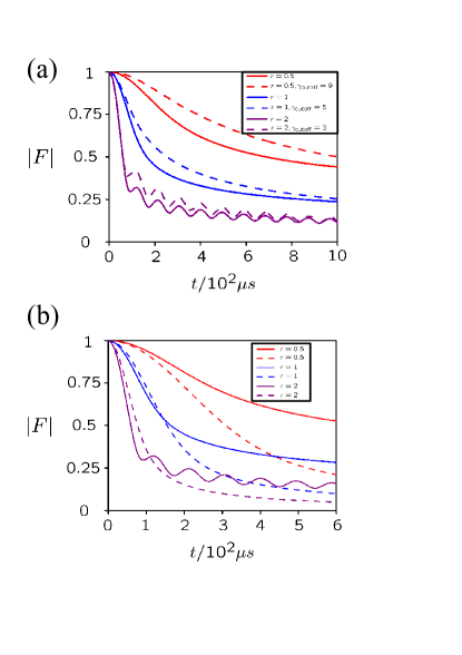
Figure 4: The decoherence factor obtained by the exact solution (solid lines) and the approximate solution (dashed lines) based on (a) Eq.(37) and (b) Eq.(39). The parameters are chosen as $N=80,\kappa=10^{-13}N/s,R=0.5\mu m,m=40m_{p}$. The temperatures are respectively $T=483nK,121nK,31nK$ to guarantee $r=0.5,1,2$ for red, blue and purple lines. And the cutoff $\gamma_{\mathrm{cutoff}}=9,5,3$ for red, blue and purple dashed lines respectively.

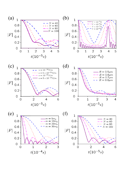
Figure 5: The evolutions of the decoherence factor for different (a)particle number $N$, (b)the temperature $T$, (c)spring constant $\kappa$, (d)the radius of the ring container $R$ and (e)the particle mass $m$. For (f), the particle number $N$ and the ring container $R$ increase simultaneously in order to keep the linear mass density $\eta=N/2\pi R$ unchanged. The basic parameters are chosen as $N=80,T=10^{-5}K,\kappa=10^{-13}N/s,R=1\mu m,m=4m_{p}$ with $m_{p}$ is mass of proton. Basically, the decoherence time is elongated for smaller particle number, lower temperature, stronger spring constant, larger ring container, and heavier particle. If the linear mass density $\eta=N/2\pi R\approx 9.55\times 10^{6}m^{-1}$ is kept unchanged and increase the particle number, the decoherenc time is elongated instead of being shortened when only the particle number is increased shown in (a). It implies that the spontaneous decoherence vanishes at the thermodynamical limit.

Eq. (37) is valid to describe the decoherence process when the thin spectrum approximately has the cosine type oscillating behavior. The contrast of the exactly decoherence factor obtained from Eq. (34) and the approximate decoherence factor in Eq. (37) are shown in Fig. 4(a) with solid lines and dashed lines, respectively. For the summation of the series of Bessel functions in Eq. (37), we need to set a cutoff of the $\gamma$. Here, we set a parameter

$$\eta=\frac{4\pi^{2}}{N^{2}\beta\Delta_{e}^{\prime}}$$ (45)

to determine the cutoff as

$$\exp\left(-\eta\gamma_{\mathrm{cutoff}}^{2}\right)=10^{-2}.$$ (46)

The parameters are chosen as $N=80,\kappa=10^{-13}N/s,R=0.5\mu m,m=40m_{p}$. The temperatures are respectively $T=483nK,121nK,31nK$ to guarantee $r=0.5,1,2$ for red, blue and purple lines. And the cutoff $\gamma_{\mathrm{cutoff}}=9,5,3$ for red, blue and purple dashed lines respectively. The approximate solution describes the decoherence process quite well for the low temperature case, where only few Bessel functions are involved contributing to the oscillating behavior of the decoherence factor.

For the relatively high temperature case such as $r<1$, Eq. (39) is valid to describe the decoherence process. The contrast of the exactly decoherence factor obtained from Eq. (34) and the approximate decoherence factor in Eq. (39) are shown in Fig. 4(b) with solid lines and dashed lines, respectively. The parameters are as same as ones used for Fig. 4(a). The decoherence processes for short time can be described quite well by Eq. (39), while the long time behavior deviate from the approximate solution because of the linear dependence of the energy difference we assumed in Eq. (38). For $\gamma>1$ the multi period contributions introduce the oscillating behavior into the decoherence factor.

Besides the temperature, the decoherence time can be elongated by adjusting other parameters such as particle number $N$, spring constant $\kappa$, the radius of the ring container $R$ and the particle mass $m$. The numerical calculation directly based on the exact solution is shown in Fig. 5. The basic parameters are chosen as $N=80,T=10^{-5}K,\kappa=10^{-13}N/s,R=1\mu m,m=4m_{p}$ with $m_{p}$ is mass of proton. From (a)-(e), the evolutions of the decoherence factor are depicted for different particle number $N$, the temperature $T$, spring constant $\kappa$, the radius of the ring container $R$ and the particle mass $m$. The spontaneous decoherence occur at first place and it is possible for the decoherence factor to revive to a relative large quantity at a later time. In some cases the revival can reach almost 1 as shown in Fig. 5(b). Such revival of the decoherence factor results from the contributions from different periods shown in Fig.  3(d), which possibly cancel each other and eventually elongate the decoherence time. If we define the decoherence time before the first possible revival, obviously it is elongated when decreasing the particle number and the temperature or increasing the spring constant, the ring container radius and the particle mass. Intriguingly, if the linear mass density $\eta=N/2\pi R$ is kept unchanged and the particle number increases just as shown in Fig. 5(f), the decoherence time is elongated instead of being shortened when only the particle number is increased shown in Fig. 5(a). It implies that the spontaneous decoherence vanishes at the thermodynamical limit, which is consistent with the textbook example of phonon in the solid state physics.

V CONCLUSION

We study the spontaneous decoherence of coupled harmonic oscillators confined in a ring container, where the nearest-neighbor harmonic potentials are taken into consideration. Without any surrounding environment, the quantum superposition state prepared in the relative degrees of freedom gradually loses its quantum decoherence. We study the spontaneous decoherence existing as the same in the closed multi-particle system when the symmetry is not broken.

The multi-particle system we study actually possesses s $U(1)\otimes C_{\mathrm{n}}$ symmetry. The Hamiltonian can be divided into the center-of-mass motion part and the relative motions part. The harmonic potentials between oscillators are periodic because of the ring configuration. Then nontrivial boundary conditions emerge to guarantee the single valuedness of the wave function, which eventually results in that the total energy spectrum not only depends on the excitations of the relative motion, but also on the total momentum corresponding to the center-of-mass motion. The consequence of the nontrivial boundary conditions is adding an additional phase factor in Eq. (15), which actually is equivalent to introducing a gauge field onto the relative motions. There is thin spectrum of the total momentum that contributes to the decoherence process. If the center-of-mass motion is not condensed to the state with single momentum, the spontaneous decoherence process occurs in the superposition states of the relative motions. Since there is no environment or symmetry breaking field at all, the decoherence in our model is definitely spontaneous.

This spontaneous decoherence is interpreted by the hidden coupling between the center-of-mass and relative degrees of freedoms. The paradox that the information represented by the coherence is always losing in a closed system can be explained by the infinite degrees of freedom of the center-of-mass motion acting like a heat bath. Especially, the spontaneous decoherence completely vanishes at the thermodynamical limit because the nontrivial boundary conditions become trivial Born-von Karman boundary condition. Our investigation shows that a thermal macroscopic object with certain symmetries has chance to degrade its quantum properties even without applying an external symmetry breaking field or surrounding environment.

Appendix A Solutions of Wave Vectors

To obtain the wave vectors $\mathbf{q}=(q_{1},q_{2,}\ldots,q_{N-1})^{T}$, we need to solve the Eq. (22). Here, $\mathbf{I}=(1,1,\ldots,1)^{T}$ and $L=2\pi R$ is the perimeter of the ring container. The matrix$\mathbf{M}$ in Eq. (22) is determined by the Fourier transforation as Eq. (4). Both the explicity forms of $\mathbf{M}$ for odd and even number $N$ can be unified written as

$$\mathbf{M}=\sqrt{\frac{2}{N}}\left[\begin{array}[]{cc}A&B\\ A^{*}&B^{*}\end{array}\right].$$ (47)

Takeing the odd number $N$ case as an example, the block matrices respectively are

$$A =\left[\begin{array}[]{c}C_{1}\\ C_{2}\\ \vdots\\ C_{\frac{N-1}{2}}\end{array}\right] ,\mbox{ }A^{*}=\left[\begin{array}[]{c}C_{\frac{N-1}{2}}\\ C_{\frac{N-3}{2}}\\ \vdots\\ C_{1}\end{array}\right],$$ (48i)

$$B =\left[\begin{array}[]{c}S_{1}\\ S_{2}\\ \vdots\\ S_{\frac{N-1}{2}}\end{array}\right] ,\mbox{ }B^{*}=-\left[\begin{array}[]{c}S_{\frac{N-1}{2}}\\ S_{\frac{N-3}{2}}\\ \vdots\\ S_{1}\end{array}\right],$$ (48r)

with row vectors

$$C_{n} = \left[\begin{array}[]{cccc}\cos\left(n\phi\right)&\cos\left(2n\phi\right)&\cdots&\cos\left(\left(\frac{N-1}{2}\right)n\phi\right)\end{array}\right],$$ (49b)

$$S_{n} = \left[\begin{array}[]{cc}-\sin\left(\left(\frac{1}{2}+n\right)\phi\right)&\sin\left(2\left(\frac{1}{2}+n\right)\phi\right)\end{array}\right.$$ (49f)

$$\left.\begin{array}[]{cc}\cdots&\left(-1\right)^{\left(\frac{N-1}{2}\right)}\sin\left(\left(\frac{N-1}{2}\right)\left(\frac{1}{2}+n\right)\phi\right)\end{array}\right],$$

$(n=1,2,\ldots,\frac{N-1}{2})$ and $\phi=2\pi/N.$ According to identities

$$\sum_{n=1}^{\frac{N-1}{2}}\cos\left(nj\phi\right)=const.$$ (50)

for any $j=1,2,\ldots,\frac{N-1}{2}$ and the fact that the wave vectors $\mathbf{q}=(q_{A},q_{B})^{T}$ can be divided into two parts according to the dimension of the block matrices, the only possible solution is $q_{A}=\left(q,q,\ldots,q\right)^{T}$ and $q_{B}=\left(0,0,\ldots,0\right)^{T}$. Therefore, the Eq. (22) is simplified as

$$qL\sqrt{\frac{2}{N}}\sum_{n=1}^{\frac{N-1}{2}}\cos\left(nm\phi\right)+\frac{2\pi n}{N}=0,$$ (51)

from which we find the solution $q=\frac{\sqrt{2}n}{\sqrt{N}R}.$

The same procedure can be applied to the case of even number N case and the solution is a little different from the odd number $N$ case as $q_{A}=\left(q,q,\ldots,q,q/2\right)^{T}$ and $q_{B}=\left(0,0,\ldots,0\right)^{T}$.

Appendix B Effective Gauge Fields on Relative Motions

The total momentum actually plays the role of the effective gauge field on the relative motions. Starting from the wavefunction obeying the Floquet theorem as Eq. (17), the original Schrodiger equation of the $k$-th relative motion

$$H_{k}\chi_{k}\left(X_{k}\right) = \epsilon_{k}\chi_{k}\left(X_{k}\right)$$ (52)

can be transformed to the Schrodinger equation of the periodic part as

$$H_{k}^{eff}u_{k}\left(X_{k}\right)=\epsilon_{k}u_{k}\left(X_{k}\right),$$ (53)

with the exactly same eigenenergy $\epsilon_{k}.$ Here, the effective Hamiltonian is obtained by a unitary transformation of the original one as

$$H_{k}^{eff} =e^{-iq_{k}X_{k}}H_{k}e^{iq_{k}X_{k}}$$

$$=\frac{\left(P_{k}+\hbar q_{k}\right)^{2}}{2m}+\frac{\kappa}{2}\left(2\sin\frac{\pi k}{N}\right)^{2}X_{k}^{2}.$$ (54)

Apprently the wave vector $q_{k}$ shifts the momentum of the relative motion, which is equivalent to an $U(1)$ gauge field. Since the wavevector $q_{k}$ linearly depends on quantum number $n$ as well as the total momentum $P_{0},$ such gauge fields on relative motions exactly results from the nonzero total momentum of the system.

Appendix C Energy Spectrum of The Periodic Harmonic Oscillator

The Schrodinger equation of the $k$-th relative motions given in Eq. (26) is described by a periodic harmonic oscillator with periodicity

$$\chi_{k}\left(X_{k}+LM_{1}^{k}\right)=e^{iq_{k}LM_{1}^{k}}\chi_{k}\left(X_{k}\right).$$ (55)

The basic idea to solve the energy spectrum in a periodic potential is solving the Schrodinger equation in a period and its adjacent period, then the wavefunctions at the interface of these two periods should satisfy the continuous condition as Eq. (27).

The wavefunction of the $k$-th relative mode is the linear combination of the two degenerate Kummer or confluent hypergeometric functions Jr08 as

$$f_{\mathrm{e}}(X_{k}) =\exp\left(-\frac{\xi_{k}^{2}X_{k}^{2}}{2}\right){}_{1}F_{1}\left[\frac{1}{4}(1-\frac{2}{\hbar\omega_{k}}\epsilon_{k});\frac{1}{2};\xi_{k}^{2}X_{k}^{2}\right],$$ (56a)

$$f_{\mathrm{o}}(X_{k}) =\xi_{k}r_{k}\exp\left(-\frac{\xi_{k}^{2}X_{k}^{2}}{2}\right){}_{1}F_{1}\left[\frac{1}{4}(3-\frac{2}{\hbar\omega_{k}}\epsilon_{k});\frac{3}{2};\xi_{k}^{2}X_{k}^{2}\right],$$ (56b)

with frequencies $\omega_{k}=2\sqrt{\kappa/m}\left|\sin\left(k\pi/N\right)\right|$ and $\xi_{k}=\sqrt{m\omega_{k}/\hbar}$. Here, the subindices $\mathbf{e}$ and $\mathbf{o}$ represent the even and odd parity, respectively. In contrast to the eigenenergy of the regular harmonic oscillator, the eigenenergy of the periodic harmonic oscillator $\epsilon_{k}$ is no longer the integer times of the frequencies $\hbar\omega_{k}$. Consequently, the wavefunction of the $k$-th relative modes within the coordinate range $X_{k}/LM_{1}^{k}\in\left[-1/2,1/2\right]$ is assumed to be

$$\chi_{k}(X_{k})=Af_{\mathrm{e}}(X_{k})+Bf_{\mathrm{o}}(X_{k})$$ (57)

with undetermined coefficients $A$ and $B$. Thus in the next period $X_{k}/LM_{1}^{k}\in\left[1/2,3/2\right]$, according to Eq.(55) the wavefunction can be written as

$$\chi_{k}(X_{k}+LM_{1}^{k})=e^{iq_{k}LM_{1}^{k}}\left[Af_{\mathrm{e}}(X_{k})+Bf_{\mathrm{o}}(X_{k})\right].$$ (58)

The continuous conditions require both the wavefunction and derivative of the wavefunction is continuous as shown in Eq. (27). Since the coefficients $A$ and $B$ can not be zero simultaneously, the determinant of the coefficients matrix of {$A,B$} should be zero as

$$\left|\begin{array}[]{cc}f_{\mathrm{e}}(-\frac{l}{2})-e^{i\theta_{k}}f_{\mathrm{e}}(\frac{l}{2})&f_{\mathrm{o}}(-\frac{l}{2})-e^{i\theta_{k}}f_{\mathrm{o}}(\frac{l}{2})\\ f_{\mathrm{e}}^{\prime}(-\frac{l}{2})-e^{i\theta_{k}}f_{\mathrm{e}}^{\prime}(\frac{l}{2})&f_{\mathrm{o}}^{\prime}(-\frac{l}{2})-e^{i\theta_{k}}f_{\mathrm{o}}^{\prime}(\frac{l}{2})\end{array}\right|=0$$ (59)

with $l=LM_{1}^{k}$, $\theta_{k}=q_{k}l$ and $f^{\prime}(a)\equiv\left.\frac{d}{dX}f(X)\right|_{X=a}$. Finaly we can obtain the constrain for the energy $\epsilon_{k}$ as

$$f_{\mathrm{o}}(\frac{l}{2})f_{\mathrm{e}}^{\prime}(\frac{l}{2})\cos^{2}\frac{\theta_{k}}{2}+f_{\mathrm{e}}(\frac{l}{2})f_{\mathrm{o}}^{\prime}(\frac{l}{2})\sin^{2}\frac{\theta_{k}}{2}=0,$$ (60)

where we have used the parity of the functions $f_{\mathrm{e}}\left(X\right)$ and $f_{\mathrm{o}}\left(X\right)$ to simplify the Eq. (59). Whether the energy spectrum depends on the total momentum or not relies on $\theta_{k}\neq 0$. Obviously, for those relative motion $k>N/2$ their energy spectrum is independent of the total momentum and thus have no contribution to the decoherence process.

The energy spectrum $\epsilon_{k}=\left(n_{k}+1/2\right)\hbar\omega_{k}$ depends on both the phase factor $\theta_{k}$ and the dimensionless parameter $\xi_{k}l$, which is shown in Fig. A1. In Fig. A1(a), the dimensionless parameter is chosen as $\xi_{k}l=5$ and the particle number is $N=100.$ Definitely, the energy spectrum depends on the phase factor $\theta_{k}=q_{k}l.$ For those relative motions with $q_{k}=0,$ the energy spectrum is only determined by the dimensionless parameter, which is determined by the geometry of the ring container and the spring constant. However, for those relative motions with $q_{k}=\frac{\sqrt{2}n}{\sqrt{N}R},$ the energy spectrum is not only depends on the total momentum now, but also form a group of thin spectrum when the total momentum chooses its possible values. In Fig. A1(b), the phase factor is chosen as $\theta_{k}=\pi/2$ and the particle number is $N=100.$ By confining the particles in a smaller ring container via decreasing $\xi_{k}l$, the energy spectrum deviates from the energy spectrum of standard harmonic oscillator greatly. When $\xi_{k}l\gg 1$ the energy spectrum is almost coincide with the standard one, which means the affect of the phase factor is also suppressed for a larger ring container or weak spring constant.

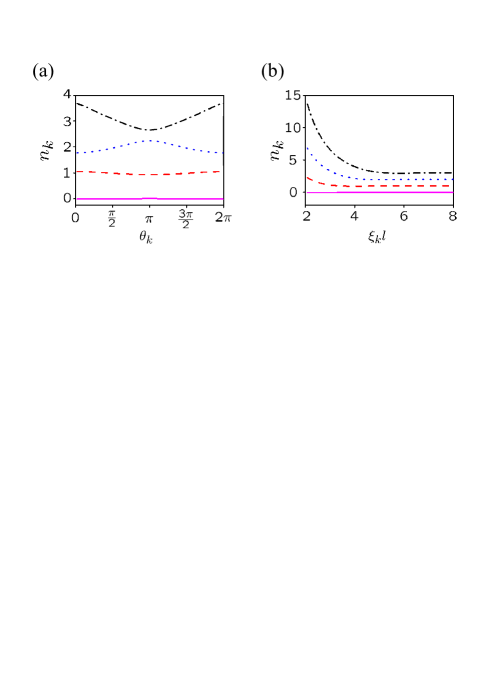
Figure 6: (Color online) (a) Energy spectrum $n_{k}$ versus phase factor $\theta_{k}$. The parameters are chosen as $N=100,\xi_{k}l=5$. (b) Energy spectrum $n_{k}$ versus the periodicity $\xi_{k}l$. The parameters are chosen as $N=100,\theta_{k}=\pi/2$. The black dotdashed line, blue dotted line, red dashed line and the magenta solid line represent the first four eigenstates of the periodic harmonic oscillator. Definitely, the energy spectrum varies with the $\theta_{k}$, implying the dependence of the total momentum. Moreover, the periodic harmonic oscillator becomes normal one when $\xi_{k}l\gg 1$ whatever $\theta_{k}$ is.

We rewrite the Eq.(60) as

$$\tan^{2}\frac{\theta_{k}}{2}=-F\left(l,\epsilon_{k}\right)$$ (61)

with

$$F\left(l,n_{k}\right)=\frac{f_{\mathrm{o}}(\frac{l}{2})f_{\mathrm{e}}^{\prime}(\frac{l}{2})}{f_{\mathrm{e}}(\frac{l}{2})f_{\mathrm{o}}^{\prime}(\frac{l}{2})}.$$ (62)

To obtain the approximate energy spectrum which depends linearly on the total momentum, we expand the Eq.(61) at the vicinity of the phase factor $\theta_{k}=\left(\frac{1}{2}+\mu\right)\pi$ and $\xi_{k}l\apprge 1.$ In this sense, the approximate energy spectrum is obtained as

$$\epsilon_{k}\left(n,\alpha\right)=\left(\frac{1}{2}+\alpha^{\prime}+\delta_{k}\left(n,\alpha\right)\right)\hbar\omega_{k},$$ (63)

where $\alpha^{\prime}$ is the solution of $F\left(l,\alpha^{\prime}\right)=-1$, $\alpha=0,1,\ldots$ is non-negative integer number and deviation

$$\delta_{k}\left(n,\alpha\right)=g_{0}\left(\alpha\right)+g_{1}\left(k,\alpha\right)n$$ (64)

with coefficients

$$g_{0}\left(\alpha\right) =-\frac{1+F\left(l,\alpha\right)+\left(-1\right)^{\mu}\left(1+2\mu\right)\pi}{G\left(l,\alpha\right)},$$ (65a)

$$g_{1}\left(k,\alpha\right) =\left(-1\right)^{\mu}2\pi\frac{M_{1}^{k}}{G\left(l,\alpha\right)}\frac{\sqrt{2}}{\sqrt{N}},$$ (65b)

and function $G\left(l,\alpha\right)\equiv\left.\frac{d}{dn_{k}}F\left(l,n_{k}\right)\right|_{n_{k}=\alpha^{\prime}}$ is the derivative of the function $F\left(l,n_{k}\right).$

- (1) W. H. Zurek, Physics Today 44,36 (1991) and reference therein.
- (2) S. Haroche, Physics Today 51,36 (1998).
- (3) W. H. Zurek, Rev. Mod. Phys. 75, 715 (2003).
- (4) C. H. Bennett and D. P. DiVincenzo, Nature (London) 404, 247 (2000).
- (5) H. T. Quan, P. Zhang, and C. P. Sun, Phys. Rev. A 73, 036122 (2006).
- (6) D. Howard, Philosophy of Science 71, 669 (2004).
- (7) O. Kübler and H. D. Zeh, Ann. Phys. (N.Y.) 76, 405 (1973).
- (8) E. Joos and H. D. Zeh, Z. Phys. B 59, 223 (1985).
- (9) H. D. Zeh, Found. Phys. 1, 69 (1970); Found. Phys. 3, 109 (1973); Phys. Lett. A 172, 189 (1993).
- (10) Zurek, W. H., Phys. Rev. D 24, 1516 (1981); Phys. Rev. D 26, 1862 (1982); Prog. Theor. Phys. 89, 281 (1993).
- (11) D. L. Zhou, P. Zhang, and C. P. Sun, Phys. Rev. A 66, 012112 (2002).
- (12) C. P. Sun, Phys. Rev. A 48, 898 (1993).
- (13) W. H. Zurek and J. P. Paz, Phys. Rev. Lett. 72, 2508 (1994).
- (14) C. P. Sun, D. L. Zhou, S. X. Yu, and X. F. Liu, Eur. Phys. J. D 13, 145 (2001); Eur. Phys. J. D 17, 85 (2001); Phys. Rev. A 63, 012111 (2001).
- (15) H. D. Zeh, The Physical Basis of the Direction of Time (Springer, Berlin), 4th edition, 2001.
- (16) E. Joos, H. D. Zeh, C. Kiefer, D. Giulini, J. Kupsch, and I.-O. Stamatescu, Decoherence and the Appearance of a Classical World in Quantum Theory (Springer, NewYork), 2nd edition, 2003.
- (17) M. Schlosshauer, Reviews of Modern Physics 76, 1267 (2005).
- (18) F. Xue, S. X. Yu, and C. P. Sun, Phys. Rev. A 73, 013403 (2006).
- (19) S. Dürr, T. Nonn, and G. Rempe, Nature 395, 33 (1998).
- (20) M. Arndt, O. Nairz, J. Vos-Andreae, C. Keller, G. van der Zouw, and A. Zeilinger, Nature 401, 680 (1999).
- (21) R. Omnès, The Interpretation of Quantum Mechanics, (Princeton University Press), 1994.
- (22) P. Zhang, X. F. Liu, and C. P. Sun, Phys. Rev. A 66, 042104 (2002).
- (23) J. van Wezel, J. van den Brink, and J. Zaanen, Phys. Rev. Lett. 94, 230401 (2005).
- (24) J. van Wezel, J. Zaanen, and J. van den Brink, Phys. Rev. B 74, 094430 (2006).
- (25) J. van Wezel, Phys. Rev. B 78, 054301 (2008).
- (26) J. van Wezel and J. van den Brink, Phys. Rev. B 77, 064523 (2008).
- (27) H. T. Quan, Z. Song, X. F. Liu, P. Zanardi, and C. P. Sun, Phys. Rev. Lett. 96, 140604 (2006).
- (28) I. Pikovski, M. Zych, F. Costa, and Caslav Brukner, Nat. Phys. 11, 668 (2015).
- (29) I. Pikovski, M. Zych, F. Costa, and Caslav Brukner, arXiv:1508.03296.
- (30) C. Gooding and W. G. Unruh, Found. Phys. 45, 1166 (2015).
- (31) N. Byers and C. N. Yang, Phys. Rev. Lett. 7, 46 (1961).
- (32) W. Magnus, S. Winkler. Hill’s Equation, Dover-Phoenix Editions (2004).
- (33) H. E. Montgomery Jr., G. Campoy, and N. Aquino, arXiv:0803.4029.