The value of timing information
in event-triggered control

Abstract

We study event-triggered control for stabilization of unstable linear plants over rate-limited communication channels subject to unknown, bounded delay. On one hand, the timing of event triggering carries implicit information about the state of the plant. On the other hand, the delay in the communication channel causes information loss, as it makes the state information available at the controller out of date. Combining these two effects, we show a phase transition behavior in the transmission rate required for stabilization using a given event-triggering strategy. For small values of the delay, the timing information carried by the triggering events is substantial, and the system can be stabilized with any positive rate. When the delay exceeds a critical threshold, the timing information alone is not enough to achieve stabilization, and the required rate grows. When the delay equals the inverse of the entropy rate of the plant, the implicit information carried by the triggering events perfectly compensates the loss of information due to the communication delay, and we recover the rate requirement prescribed by the data-rate theorem. We also provide an explicit construction yielding a sufficient rate for stabilization, as well as results for vector systems. Our results do not rely on any a priori probabilistic model for the delay or the initial conditions.

I Introduction

Cyber-physical systems (CPS) are engineering systems that integrate computing, communication, and control. They arise in a wide range of areas such as robotics, energy, civil infrastructure, manufacturing, and transportation [3, 4]. Due to the need for tight integration of different components, requirements and time scales, the modeling, analysis, and design of CPS present new challenges. One key aspect is the presence of finite-rate, digital communication channels in the feedback loop. Data-rate theorems quantify the effect that communication has on stabilization by stating that the communication rate available in the feedback loop should be at least as large as the intrinsic entropy rate of the system (corresponding to the sum of the logarithms of the unstable modes). In this way, the controller can compensate for the expansion of the state occurring during the communication process. Early formulations of data-rate theorems appeared in [5, 6, 7], followed by the key contributions in [8, 9]. More recent extensions include time-varying rate, Markovian, erasure, additive white and colored Gaussian, and multiplicative noise feedback communication channels [10, 11, 12, 13, 14, 15, 16], formulations for nonlinear systems [17, 18, 19], for optimal control [20, 21, 22], for systems with random parameters [23, 24, 25], and for switching systems [26, 27]. Connections with information theory are highlighted in [19, 28, 29, 30, 31]. Extended surveys of the literature appear in [32, 33] and in the book [34].

Another key aspect of CPS to which we pay special attention here is the need to efficiently use the available resources. Event-triggering control techniques [35, 36, 37] have emerged as a way of trading computation and decision-making for other services, such as communication, sensing, and actuation. In the context of communication, event-triggered control seeks to prescribe information exchange between the controller and the plant in an opportunistic manner. In this way, communication occurs only when needed for the task at hand (e.g., stabilization, tracking), and the primary focus is on minimizing the number of transmissions while guaranteeing the control objectives and the feasibility of the resulting real-time implementation. While the majority of this literature relies on the assumption of continuous availability and infinite precision of the communication channel, recent works also explore event-triggered implementations in the presence of data-rate constraints [38, 39, 40, 41, 42, 43], and packet drops [44, 45, 46]. In this context, one important observation raised in [39] is that using event-triggering it is possible to “beat” the data-rate theorem. Namely, if the channel does not introduce any delay and the controller knows the triggering mechanism, then an event-triggering strategy can achieve stabilization for any positive rate of transmission. This apparent contradiction can be explained by noting that the timing of the triggering events carries information, revealing the state of the system. When communication occurs without delay, the controller can track the state with arbitrary precision, and transmitting a single data payload bit at every triggering event is enough to compute the appropriate control action. The works [39, 40] take advantage of this observation to show that any positive rate of transmission is sufficient for stabilization when the delay is sufficiently small. In contrast, the work in [38] studies the problem of stabilization using an event-triggered strategy, but it does not exploit the implicit timing information carried by the triggering events. The recent work in [47] studies the required information transmission rate for containability [6] of scalar systems, when the delay in the communication channel is at most the inverse of the intrinsic system’s entropy rate. Finally,  [2] compares the results presented here with those of a time-triggered implementation.

The main contribution of this paper is the precise quantification of the amount of information implicit in the timing of the triggering events across the whole spectrum of possible communication delay values, and the use of both timing information and data payload for stabilization. For a given event-triggering strategy, we derive necessary and sufficient conditions for the exponential convergence of the state estimation error and the stabilization of the plant, revealing a phase transition behavior of the transmission rate as a function of the delay. Key to our analysis is the distinction between the information access rate, that is the rate at which the controller needs to receive information, conveyed by both data payload and timing information and regulated by the classic data-rate theorem; and the information transmission rate, that is the rate at which the sensor needs to send data payload, that is affected by channel delays, as well as design choices such as event-triggering or time-triggering strategies. We show that for sufficiently low values of the delay, the timing information carried by the triggering events is large enough and the system can be stabilized with any positive information transmission rate. At a critical value of the delay, the timing information carried by the triggering events is not enough for stabilization, and the required information transmission rate begins to grow. When the delay reaches the inverse of the entropy rate of the plant, the timing information becomes completely obsolete, and the required information transmission rate becomes larger than the information access rate imposed by the data-rate theorem. We also provide necessary conditions on the information access rate for asymptotic stabilizability and observability with exponential convergence guarantees; necessary conditions on the information transmission rate for asymptotic observability with exponential convergence guarantees; as well as a sufficient condition with the same asymptotic behavior. We consider both scalar and vector linear systems without disturbances. Extensions for future work include the consideration of disturbances and the analysis under triggering strategies different from the one considered here.

Notation

Let $\mathbb{R}$, $\mathbb{Z}$ and $\mathbb{N}$ denote the set of real numbers, integers, and positive integers, respectively. We denote by $\mathcal{B}(r)$ the ball centered at $0$ of radius $r$. We let $\log$ and $\ln$ denote the logarithm with bases $2$ and $e$, respectively. For a function $f:\mathbb{R}\rightarrow\mathbb{R}^{n}$ and $t\in\mathbb{R}$, we let $f(t^{+})$ denote the limit from the right, namely $\lim_{s\downarrow t}f(s)$. We let $M_{n,m}(\mathbb{R})$ be the set of $n\times m$ matrices over the field of real numbers. Given $A=[a_{i,j}]_{1\leq i,j\leq n}\in M_{n,n}(\mathbb{R})$, we let $\operatorname*{\operatorname{Tr}}(A)=\sum_{i=1}^{n}a_{ii}$ and $\det(A)$ denote its trace and determinant, respectively. We let $m$ denote the Lebesgue measure on $\mathbb{\mathbb{R}}^{n}$, which for $n=2$ and $n=3$ can be interpreted as area and volume, respectively. We let $\lfloor x\rfloor$ denote the greatest integer less than or equal to $x$, and $\lceil x\rceil$ denote the smallest integer greater than or equal to $x$. We denote by $\text{mod}(x,y)$ the modulo function, whose value is the remainder left after dividing $x$ by $y$. We let $\|x\|$ be the $L^{2}$ norm of $x$ in $\mathbb{R}^{n}$. We let $\text{sign}(x)$ be $1$, $-1$, or $0$ when $x$ is positive, negative, or zero, respectively.

II Problem formulation

Here we describe the system evolution, the model for the communication channel, and the event-triggering strategy.

II-A System model

We consider the standard networked control system model composed of the plant-sensor-channel-controller tuple depicted in Figure 1. We start with a scalar, continuous-time, linear time-invariant (LTI) system, and then extend the model to the vector case.

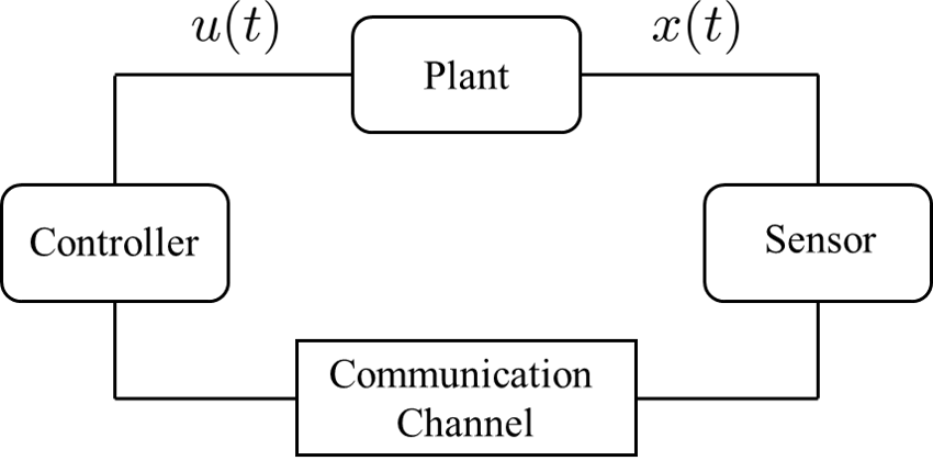
Figure 1: System model. The sensor can measure the full state of the system and the controller applies the input with infinite precision and without delay. The communication channel only supports a finite rate and is subject to delay.

The plant dynamics are described by

$$\dot{x}(t)=Ax(t)+Bu(t),$$ (1)

where $x(t)\in\mathbb{R}$ and $u(t)\in\mathbb{R}$ for $t\in[0,\infty)$ are the system state and control input, respectively. Here, $A$ is a positive real number, $B$ is a nonzero real number, and $|x(0)|<L$ is any bounded initial condition, where $L$ is known to both sensor and controller. The sensor can measure the state of the system perfectly, and the controller can apply the control input with infinite precision and without delay. However, the sensor and the controller communicate through a channel that can support only a finite communication rate and is subject to delay. At each triggering event, the sensor can transmit a packet composed of a finite number of bits, representing a quantized version of the state, through the communication channel, which is received by the controller entirely and without error, after an unknown, bounded delay, as described next.

II-B Triggering strategy and controller dynamics

We denote by $\{t_{s}^{k}\}_{k\in\mathbb{N}}$ the sequence of times at which the sensor transmits to the controller a packet composed of $g(t_{s}^{k})$ bits representing the state of the plant. For every $k\in\mathbb{N}$, we let $t_{c}^{k}$ be the time at which the controller receives the packet that the sensor transmitted at time $t_{s}^{k}$. We assume a uniform upper bound, known to both the sensor and the controller, on the unknown communication delays

$$\Delta_{k}=t_{c}^{k}-t_{s}^{k}\leq\gamma,$$ (2)

and denote the $k^{\text{th}}$ triggering interval by

$$\Delta^{\prime}_{k}=t_{s}^{k+1}-t_{s}^{k}.$$

We assume the upper bound on the communication delays in (2) to be independent of the packet size. When referring to a generic triggering time or reception time, for notational convenience we omit the superscript $k$ in $t_{s}^{k}$ and $t_{c}^{k}$. Our model does not assume any a priori probability distribution for the delay, and our results hold for any random communication delay with bounded support.

From the data received from the sensor, and from the timing at which the data is received, the controller maintains an estimate $\hat{x}$ of the plant state, which starting from $\hat{x}(t_{c}^{k+})$ evolves during the inter-reception times as

$$\dot{\hat{x}}(t)=A\hat{x}(t)+Bu(t),\quad t\in[t_{c}^{k},t_{c}^{k+1}].$$ (3)

The controller then computes the control input $u(t)$ based on this estimate. The sensor can compute the same estimate $\hat{x}(t)$ for the plant state at the controller via communication through the control input [28]. Namely, assuming that the input has been computed by the controller as $u(t)=\mu(\hat{x}(t))$, where $\mu$ an invertible function known to both parties, the sensor can first compute $u(t)=(\dot{x}(t)-Ax(t))/B$ and then compute $\hat{x}(t)$ by inversion.

The state estimation error computed at the sensor is then

$$z(t)=x(t)-\hat{x}(t).$$

Initially, we let $x(0)-\hat{x}_{0}=z(0)$. Without updated information from the sensor, this error grows, and the system can potentially become unstable. The sensor should, therefore, select the sequence of transmission times $\{t_{s}^{k}\}_{k\in\mathbb{N}}$, the packet sizes $\{g(t^{k}_{s})\}_{k\in\mathbb{N}}$ and the corresponding quantization strategy used to determine the data payload, so that the controller can ensure stability. This choice requires a certain communication rate available in the channel, which we wish to characterize.

To select the transmission times, we adopt an event-triggering approach. Consider the event-triggering function known to both sensor and controller

$$v(t)=v_{0}e^{-\sigma t},$$ (4)

where $v_{0}$ and $\sigma$ are positive real numbers. A transmission occurs whenever

$$|z(t)| =v(t).$$ (5)

Upon reception of the packet, the controller updates the estimate of the state according to the jump strategy

$$\hat{x}(t_{c}^{+})=\bar{z}(t_{c})+\hat{x}(t_{c}),$$ (6)

where $\bar{z}(t_{c})$ is an estimate of ${z}(t_{c})$ constructed by the controller knowing that $|z(t_{s})|=v(t_{s})$, the bound (2), and the decoded packet received through the communication channel. It follows that

$$|z(t_{c}^{+})|=|x(t_{c})-\hat{x}(t_{c}^{+})|=|z(t_{c})-\bar{z}(t_{c})|.$$

We also point out that if the control law is not invertible, the sensor can perform the same computation of the controller to obtain $\hat{x}(t_{c}^{+})$, provided that it can infer the reception times from jumps in the control input.

By transmitting when the state estimation error $|z(t)|$ reaches the threshold $|v(t)|$, the sensor effectively encodes information in timing using the event-triggering rule (5). On the other hand, the data payload of the transmissions also carries information, and the sensor can choose any arbitrary, finite-precision quantization of the state to construct the data payload as long as it ensures that, for all $t_{c}\in[t_{s},t_{s}+\gamma]$,

$$|z(t_{c}^{+})|=|z(t_{c})-\bar{z}(t_{c})|\leq\rho(t_{s}):=\rho_{0}e^{-\sigma\gamma}v(t_{s}),$$ (7)

where $0<\rho_{0}<1$ is a given design parameter. Note that $v(t_{c})=v_{0}e^{-\sigma t_{c}}\geq v_{0}e^{-\sigma t_{s}}e^{-\sigma\gamma}=v(t_{s})e^{-\sigma\gamma}$, and hence (7) ensures that at each triggering event the estimation error drops below the triggering function, namely

$$|z(t_{c}^{+})| \leq\rho_{0}v(t_{c}).$$

Consequently, the sequence of transmission times $\{t_{s}^{k}\}_{k\in\mathbb{N}}$ is monotonically increasing, i.e., $\Delta^{\prime}_{k}>0$ for all $k\in\mathbb{N}$. Moreover, based on $\dot{z}=Az$ and (5), a new transmission occurs only after the previous packet has been delivered to the controller, that is $t_{s}^{k+1}>t_{c}^{k}$. Additionally, using $\dot{z}=Az$ and (2), we deduce

$$|z(t_{c})| \leq v(t_{s})e^{A\gamma}\leq v_{0}e^{-\sigma(t_{c}-\gamma)}e^{A\gamma}$$

$$=v_{0}e^{(A+\sigma)\gamma}e^{-\sigma t_{c}}.$$ (8)

From (7) and (8), it follows that the described triggering strategy ensures an exponentially decaying estimation error. The design parameter $\rho_{0}$ regulates the resolution of the quantization, and hence the size of the transmitted packets; as well as the magnitude of the jumps below the triggering function, and hence the triggering rate. These also depend on the delay, which governs the amount of overshoot of the estimation error above the triggering function, see Figure 2.

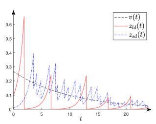
Figure 2: Evolution of the state estimation error $|z_{ld}(t)|$ for a larger delay upper bound $\gamma=1.2$, and $|z_{sd}(t)|$ for a smaller delay upper bound $\gamma=0.9$. Here, $A=1$, $\sigma=0.1$, and $\rho_{0}=0.1$. The dashed exponential decaying curve represents the triggering function $v(t)=0.27e^{-\sigma t}$. A larger delay corresponds to a larger overshoot of the estimation error above the triggering function and higher uncertainty about the state at the controller. Since $\gamma$ regulates the resolution of the quantization (7) in an exponential manner, larger delay corresponds to larger jumps under the triggering function upon reception of the packet.

The design parameter $v_{0}$ determines the initial condition of the estimation error when the first triggering event occurs. For any given $0<\rho_{0}<1$, and $0<v_{0}<\infty$, our objective is to determine the rate required to achieve these exponential bounds for all possible delay realizations, and then provide an explicit quantization strategy that satisfies these bounds.

II-C Information transmission rate

To define the transmission rate, we take the viewpoint of the sensor and examine the amount of information that it needs to transmit so that the controller is able to stabilize the system. Let $b_{s}(t)$ be the number of bits in the data payload transmitted by the sensor up to time $t$, and define the information transmission rate as

$$R_{s}=\limsup_{t\rightarrow\infty}\frac{b_{s}(t)}{t}.$$

Since at every triggering time, $t_{s}^{k}$ the sensor sends $g(t_{s}^{k})$ data payload bits, we have

$$R_{s}=\limsup_{N\rightarrow\infty}\frac{\sum_{k=1}^{N}g(t_{s}^{k})}{\sum_{k=1}^{N}\Delta^{\prime}_{k}}.$$

We now make two key observations. First, in the presence of unknown communication delays, the state estimate received by the controller might be out of date so that the sensor might need to send data at a higher rate than what is needed on a channel without delay. Second, in the presence of event-triggered transmissions, the timing of the triggering events carries implicit information. For example, if the communication channel does not introduce any delay, and assuming that the sensor and the controller can keep track of time with infinite precision, then the time of a triggering event reveals the system state up to a sign, since according to (5),

$$x(t)=\hat{x}(t)\pm v(t).$$

It follows that in this case, the controller can stabilize the system even if the sensor uses the channel very sparingly, transmitting a single data payload bit at a triggering event, that is at a much smaller rate than what needed in any time-triggered implementation. In general, there is a trade-off between the information gain due to triggering timing, and the information loss due to the delay. As we shall see below, this leads to a phase transition in the minimum rate required to satisfy (7) and as a consequence (8).

Finally, it is worth pointing out that the exponential convergence of the state estimation error to zero implies the asymptotic stabilizability of the system.

II-D Information access rate

We now consider the viewpoint of the controller and examine the amount of information that it needs to receive from the plant to be able to stabilize the system. We define $b_{c}(t)$ to be the amount of information, measured in bits, conveyed by both data payload and timing information, received by the controller up to time $t$. We define the information access rate as

$$R_{c}=\limsup_{t\rightarrow\infty}\frac{b_{c}(t)}{t}.$$

Classic data-rate theorems describe the information access rate required to stabilize the system. They are generally stated for discrete-time systems, albeit similar results hold in continuous time as well, see e.g. [48]. They are based on the fundamental observation that there is an inherent entropy rate

$$h=\frac{A}{\ln 2},$$

at which the system generates information. It follows that for the system to be stabilizable the controller must have access to state information at a rate

$$R_{c}\geq h.$$ (9)

This result indicates what is required by the controller, and it does not depend on the feedback structure — including aspects such as communication delays, information pattern at the sensor and the controller, and whether the times at which transmissions occur are state-dependent, as in event-triggered control, or periodic, as in time-triggered control.

III Necessary condition on the access rate

In this section, we quantify the amount of information that the controller needs to ensure exponential convergence of the state estimation error or the state to zero, independently of the feedback structure used by the sensor to decide when to transmit. The result obtained here generalizes (9) and establishes a common ground to compare later against the results for the information transmission rate, which depend on the given policy adopted by the sensor. The proof follows, with minor modifications, the argument in [8, Propositions $3.1$ and $3.2$] for discrete-time systems.

Theorem 1.

Consider the plant-sensor-channel-controller model described in Section II, with plant dynamics (1), and state estimation error $z(t)$, and let $\sigma>0$. The following necessary conditions hold:

1. If the state estimation error satisfies

   $$|z(t)|\leq|z(0)|~{}e^{-\sigma t},$$

   then

   $$b_{c}(t)\geq t~{}\frac{A+\sigma}{\ln 2}+~{}\log\frac{L}{|z(0)|}.$$ (10)

2. If the system is stabilizable and

   $$|x(t)|\leq|x(0)|~{}e^{-\sigma t},$$

   then

   $$b_{c}(t)\geq t~{}\frac{A+\sigma}{\ln 2}.$$ (11)

In both cases, the necessary information access rate is

$$R_{c}\geq\frac{A+\sigma}{\ln 2}.$$ (12)

Proof.

From (1), we have

$$x(t) =e^{At}x(0)+\alpha(t),$$ (13a)

$$\alpha(t) =e^{At}\int_{0}^{t}{e^{-A\tau}Bu(\tau)d\tau}.$$ (13b)

Using (13a) we define the uncertainty set at time $t$

$$\Gamma_{t}=\{x\in\mathbb{R}:x=e^{At}x(0)+\alpha(t)\text{ and }x(0)\in\mathcal{B}(L)\}.$$

The state of the system can be any point in this uncertainty set. Letting $\epsilon(t)=|z(0)|~{}e^{-\sigma t}$, we can then find a lower bound on $b_{c}(t)$ by counting the number of one-dimensional balls of radius $\epsilon(t)$ that cover $\Gamma_{t}$. Specifically,

$$b_{c}(t) \geq\log\frac{m(\Gamma_{t})}{m(\mathcal{B}(\epsilon(t)))}=\log\frac{e^{At}m(\mathcal{B}(L))}{2|z(0)|~{}e^{-\sigma t}}$$

$$=t~{}\log e^{A+\sigma}+\log\frac{L}{|z(0)|},$$

which proves (i).

To prove (ii), for any given control trajectory $\{u(\tau)\}_{\tau\in[0,t]}$, define the set of initial conditions for which the plant state $x(t)$ tends to zero exponentially with rate $\sigma$, i.e.,

$$\Pi_{\{u(\tau)\}_{\tau\in[0,t]}}=\{x(0)\in\mathcal{B}(L):|x(t)|\leq|x(0)|~{}e^{-\sigma t}\}.$$

By (13b) $x(t)$ depends linearly on $\{u(\tau)\}_{\tau\in[0,t]}$, so that all the sets $\Pi_{\{u(\tau)\}_{\tau\in[0,t]}}$ are linear transformations of each other. The measure of $\Pi_{\{u(\tau)=0\}_{\tau\in[0,t]}}$ is $2|x(0)|e^{-At}e^{-\sigma t}$, which is upper bounded by $2Le^{-At}e^{-\sigma t}$. Hence, this quantity also upper bounds the measure of each $\Pi_{\{u(\tau)\}_{\tau\in[0,t]}}$. It follows that we can determine a lower bound for $b_{c}(t)$ by counting the number of sets of measure $2Le^{-At}e^{-\sigma t}$ required to cover the ball $|x(0)|\leq L$, and we have

$$b_{c}(t) \geq\log\frac{2L}{2Le^{-(A+\sigma)t}}=t~{}\frac{A+\sigma}{\ln 2},$$

showing (ii). Finally, (12) follows by dividing (10) and (11) by $t$ and taking the limit for $t\rightarrow\infty$. ∎

Remark 1.

Theorem 1 is valid for any control scheme, and the controller does not necessarily have to compute the state estimate following (3). This result can be viewed as an extension of the data-rate theorem with exponential convergence guarantees. It states that to have exponential convergence of the estimation error and the state, the access rate should be larger than the estimation entropy, the latter concept having been recently introduced in [49]. A similar result for continuous-time systems appears in [38], but only for linear feedback controllers. In fact, this work shows that the bound in (12) is also sufficient for scalar systems when the controller does not use any timing information about the triggering events. The classic formula of the data-rate theorem (9) [8, 9], can be derived as a special case of Theorem 1 by taking $\sigma\rightarrow 0$ and using continuity. $\bullet$

IV Necessary and sufficient conditions on the transmission rate

In this section, we determine necessary and sufficient conditions on the transmission rate for the exponential convergence of the estimation error under the event-triggered control strategy described in Section II. We start by observing that in an event-triggering implementation, the transmission times and the packet sizes are state-dependent. Thus, there may be some initial conditions and delay realizations for which both the necessary and sufficient transmission rates are arbitrarily small. For this reason, we provide results that hold in worst-case conditions, namely accounting for all possible realizations of the delay and initial conditions, without assuming any a priori distribution on these realizations.

IV-A Necessary condition on the transmission rate

Here we quantify the necessary rate at which the sensor needs to transmit to ensure the exponential convergence of the estimation error to zero under the given event-triggering strategy. This rate depends on the number of bits that the sensor transmits at each triggering event, as well as the frequency with which transmission events occur, according to the triggering rule. Our strategy to obtain a necessary rate consists of appropriately bounding each of these quantities.

To obtain a lower bound on the number of bits transmitted at each triggering event, consider the uncertainty set of the sensor about the estimation error at the controller, $z(t_{c})$, given $t_{s}$

$$\Omega(z(t_{c})|t_{s})=\{y:y=\pm v(t_{s})e^{A(t_{c}-{t}_{s})},\ t_{c}\in[t_{s},t_{s}+\gamma]\}.$$

On the other hand, consider the uncertainty from the point of view of the controller about $z(t_{c})$, given $t_{c}$

$$\Omega(z(t_{c})|t_{c}) =\{y:y=\pm v(\bar{t}_{r})e^{A(t_{c}-\bar{t}_{r})},\ \bar{t}_{r}\in[t_{c}-\gamma,t_{c}]\}.$$

Clearly, for any $t_{c}\in[t_{s},t_{s}+\gamma]$, we have $\Omega(z(t_{c})|t_{c})\neq\Omega(z(t_{c})|t_{s})$, namely there is a mismatch between the uncertainties at the controller and at the sensor. The next result shows that the uncertainty at the sensor is always smaller than the one at the controller.

Lemma 1.

Consider the plant-sensor-channel-controller model described in Section II, with plant dynamics (1), estimator dynamics (3), event-triggering function (4), triggering strategy (5), and jump strategy (6). Then, $\Omega(z(t_{c})|t_{s})\subseteq\Omega(z(t_{c})|t_{c})$.

Proof.

The uncertainty set of the sensor can be expressed as

$$\Omega(z(t_{c})|t_{s})=[v(t_{s}),v(t_{s})e^{A\gamma}]\cup[-v(t_{s})e^{A\gamma},-v(t_{s})].$$

Noting that for any $t_{c}\in[t_{s},t_{s}+\gamma]$, $v(\bar{t}_{r})e^{A(t_{c}-\bar{t}_{r})}$ is a decreasing function of $\bar{t}_{r}$, we have

$$\Omega( z(t_{c})|t_{c})=$$

$$[v(t_{c}),v(t_{c})e^{(A+\sigma)\gamma}]\cup[-v(t_{c})e^{(A+\sigma)\gamma},-v(t_{c})].$$

The result now follows by noting that, since $v$ is a decreasing function, for all $t_{c}\in[t_{s},t_{s}+\gamma]$ we have $v(t_{s})\geq v(t_{c})$ and $v(t_{s})e^{A\gamma}\leq v(t_{c})e^{(A+\sigma)\gamma}$. ∎

To ensure that (7) holds, the controller needs to reduce the state estimation error $z(t_{c})$ to within an interval of radius $\rho(t_{s})$. From Lemma 1, this implies that the sensor needs to cover at least the uncertainty set $\Omega(z(t_{c})|t_{s})$ with one-dimensional balls of radius $\rho(t_{s})$. This observation leads us to the following lower bound on the number of bits that the sensor must transmit at every triggering event.

Lemma 2.

Under the assumptions of Lemma 1, if (7) holds for all $k\in\mathbb{N}$, then the packet size at every triggering event must satisfy

$$g(t_{s}^{k})\geq\max\left\{0,\log\frac{(e^{A\gamma}-1)}{\rho_{0}e^{-\sigma\gamma}}\right\}.$$ (14)

Proof.

We compute the number of bits that must be transmitted to guarantee that the sensor uncertainty set $\Omega(z(t_{c})|t_{s})$ is covered by balls of radius $\rho(t_{s})$. Define $\chi_{\gamma}=\{y:y=e^{At},t\in[0,\gamma]\}$. Since $g(t_{s})$ is the packet size, it is non-negative. Hence, $g(t_{s})\geq\max\left\{0,H_{\rho(t_{s})}\right\}$, where

$$H_{\rho(t_{s})} :=\log\frac{m(\Omega(z(t_{c})|t_{s}))}{m(\mathcal{B}(\rho(t_{s})))}$$

$$=\log\frac{2v(t_{s})m(\chi_{\gamma})}{2\rho_{0}e^{-\sigma\gamma}v(t_{s})}$$

$$=\log\frac{2v(t_{s})(e^{A\gamma}-1)}{2\rho_{0}e^{-\sigma\gamma}v(t_{s})},$$ (15)

and the result follows. ∎

Our next goal is to characterize the frequency with which transmission events are triggered. We define the triggering rate

$$R_{tr} =\limsup_{N\rightarrow\infty}\frac{N}{\sum_{k=1}^{N}\Delta^{\prime}_{k}}.$$ (16)

First, we provide an upper bound on the triggering rate that holds for all initial conditions and possible communication delays upper bounded by $\gamma$.

Lemma 3.

Under the assumptions of Lemma 1, if (7) holds for all $k\in\mathbb{N}$, then the triggering rate is upper bounded as

$$R_{tr}\leq\frac{A+\sigma}{-\ln(\rho_{0}e^{-\sigma\gamma})}.$$ (17)

Proof.

Consider two successive triggering times $t_{s}^{k}$ and $t_{s}^{k+1}$ and the reception time $t_{c}^{k}$. We have $t_{s}^{k}\leq t_{c}^{k}\leq t_{s}^{k+1}$. From (1) and (3), we have $\dot{z}(t)=A(x(t)-\hat{x}(t))=Az(t)$. The triggering time $t_{s}^{k+1}$ is defined by

$$|z(t_{c}^{k+})e^{A(t_{s}^{k+1}-t_{c}^{k})}|=v(t_{s}^{k+1}).$$ (18)

From (7), we have

$$\rho_{0}e^{-\sigma\gamma}v(t_{s}^{k})e^{A(t_{s}^{k+1}-t_{c}^{k})}\geq v(t_{s}^{k+1}).$$

Using (4) and $t_{s}^{k}\leq t_{c}^{k}$, it follows that

$$\rho_{0}e^{-\sigma\gamma}v_{0}e^{-\sigma t_{s}^{k}}e^{A(t_{s}^{k+1}-t_{s}^{k})}\geq v_{0}e^{-\sigma t_{s}^{k+1}},$$

and after some algebra we obtain

$$(A+\sigma)(t_{s}^{k+1}-t_{s}^{k})\geq-\ln(\rho_{0}e^{-\sigma\gamma}).$$

We then have the uniform lower bound for all $k\in\mathbb{N}$

$$\Delta^{\prime}_{k}=t_{s}^{k+1}-t_{s}^{k}\geq\frac{-\ln(\rho_{0}e^{-\sigma\gamma})}{A+\sigma},$$ (19)

which substituted into (16) leads to the desired upper bound on the triggering rate. ∎

Remark 2.

In addition to providing an upper bound on the triggering rate, Lemma 3 also shows that our event-triggered scheme does not exhibit “Zeno behavior” [50], namely the occurrence of infinitely many triggering events in a finite time interval. This follows from the uniform lower bound for all $k\in\mathbb{N}$ on the size of triggering interval in (19). $\bullet$

If $\Delta_{k}=0$ and $|z(t_{c}^{k+})|=\rho_{0}e^{-\sigma\gamma}v(t_{s})$ for all $k\in\mathbb{N}$, then the upper bound on the triggering rate in Lemma 3 is tight. Our next goal is to provide a lower bound on the triggering rate that holds for a given initial condition and delay value. To obtain a nontrivial lower bound, we need to restrict the class of allowed quantization policies used to construct the data payload. We assume that, at each triggering event, there exists a delay such that the sensor can reduce the estimation error at the controller to at most a fraction of the maximum value $\rho(t_{s})$ required by (7). This is a natural assumption, and in practice corresponds to assuming an upper bound on the size of the packet that the sensor can transmit at every triggering event and hence on the precision of the quantization strategy. Without such a bound, a packet may carry an unlimited amount of information, the quantization error may become arbitrary small, and $|z(t_{c}^{+})|$ may become arbitrarily close to zero for all delay values, resulting in a triggering rate arbitrarily close to zero. The next assumption precludes such an unrealistic scenario.

Assumption 1.

The controller can only achieve $\nu$-precision quantization. Formally, letting $\beta=\frac{1}{A}\ln(1+2\rho_{0}e^{-\sigma\gamma})$, we assume there exists a delay realization $\{\Delta_{k}\leq\beta\}_{k\in\mathbb{N}}$, an initial condition $x(0)$, and a real number $\nu\geq 1$, such that for all $k\in\mathbb{N}$

$$|z(t_{c}^{k})-\bar{z}(t_{c}^{k})|\geq\frac{\rho(t_{s}^{k})}{\nu}.$$ (20)

The upper bound $\beta$ on the delay in Assumption 1 corresponds to the time required for the state estimation error to grow from $z(t_{s})$ to $z(t_{s})+2\rho(t_{s})$. In fact,

$$z(t_{c}) =z(t_{s})e^{A\beta}=z(t_{s})(1+2\rho_{0}e^{-\sigma\gamma}),$$

from which it follows that

$$z(t_{c})-z(t_{s})=2z(t_{s})\rho_{0}e^{-\sigma\gamma},$$

and since $z(t_{s})=\pm v(t_{s})$, we have

$$|z(t_{c})-z(t_{s})|=2\rho(t_{s}).$$

To ensure (7), the size of the quantization cell should be at most $2\rho(t_{s})$. As the delay takes values in $[0,\beta]$, the value of $z(t_{c})$ sweeps an area of measure $2\rho(t_{s})$. It follows that Assumption 1 corresponds to the existence of a value of the communication delay for which the uncertainty ball about the state shrinks from having a radius at most $\rho(t_{s})$ to having a radius at least $\rho(t_{s})/\nu$. With this assumption in place, we can now compute the desired lower bound on the triggering rate.

Lemma 4.

Under the assumptions of Lemma 1, if (7) holds with $\nu$-precision for all $k\in\mathbb{N}$, then there exists a delay realization $\{\Delta_{k}\}_{k\in\mathbb{N}}$ and an initial condition such that

$$R_{tr}\geq\frac{A+\sigma}{\ln\nu+\ln(2+\frac{e^{\sigma\gamma}}{\rho_{0}})}.$$

Proof.

By Assumption 1, for all $k\in\mathbb{N}$ there exists a delay $\Delta_{k}\leq\beta$ such that

$$|z(t_{c}^{k+})|\geq(1/\nu)\rho_{0}v(t_{s}^{k})e^{-\sigma\gamma}.$$

From the definition of the triggering time $t_{s}^{k+1}$ in (18), we also have

$$(1/\nu)\rho_{0}e^{-\sigma\gamma}v(t_{s}^{k})e^{A(t_{s}^{k+1}-t_{s}^{k}-\Delta_{k})}\leq v(t_{s}^{k+1}).$$

Noting that for all $k\in\mathbb{N}$, $\Delta_{k}\leq\beta$, we have

$$(1/\nu)\rho_{0}e^{-\sigma\gamma}v(t_{s}^{k})e^{A(t_{s}^{k+1}-t_{s}^{k}-\beta)}\leq v(t_{s}^{k+1}).$$

By dividing both sides by $(1/\nu)\rho_{0}e^{-\sigma\gamma}$ and using the definition of triggering function, we obtain

$$e^{(A+\sigma)(t_{s}^{k+1}-t_{s}^{k})}\leq\frac{1}{(1/\nu)\rho_{0}e^{-\sigma\gamma}e^{-A\beta}}.$$

Taking the logarithm, we get

$$\Delta_{k}^{\prime}=t_{s}^{k+1}-t_{s}^{k}\leq\frac{-\ln((1/\nu)\rho_{0}e^{-\sigma\gamma})+A\beta}{A+\sigma}.$$ (21)

By substituting (21) into (16), we finally have

$$R_{tr} \geq\lim_{N\rightarrow\infty}\frac{1}{\frac{-\ln((1/\nu)\rho_{0}e^{-\sigma\gamma})}{A+\sigma}+\frac{A}{A+\sigma}\beta}$$

$$=\frac{A+\sigma}{\ln\nu-\ln(\rho_{0}e^{-\sigma\gamma})+\ln(1+2\rho_{0}e^{-\sigma\gamma})}$$

$$=\frac{A+\sigma}{\ln\nu+\ln(2+\frac{e^{\sigma\gamma}}{\rho_{0}})}.$$

∎

We can now combine Lemma 2 and Lemma 4 to obtain a lower bound on the information transmission rate.

Theorem 2.

Under the assumptions of Lemma 1, if (7) holds with $\nu$-precision for all $k\in\mathbb{N}$, then there exists a delay realization $\{\Delta_{k}\}_{k\in\mathbb{N}}$ and an initial condition such that

$$R_{s}\geq\frac{A+\sigma}{\ln\nu+\ln(2+\frac{e^{\sigma\gamma}}{\rho_{0}})}\max\left\{0,\log\frac{(e^{A\gamma}-1)}{\rho_{0}e^{-\sigma\gamma}}\right\}.$$ (22)

Remark 3.

Theorem 2 provides a necessary transmission rate for the exponential convergence of the estimation error to zero using our event-triggering strategy. By noting that the lower bound in (22) does not depend on $v_{0}$, it is easy to check that as $\sigma\rightarrow 0$, this result also gives a necessary condition for asymptotic stability, although it does not provide an exponential convergence guarantee of the state. $\bullet$

IV-B Phase transition behavior

We now show a phase transition for the rate required for stabilization expressed in Theorem 2. By combining Lemmas 3 and 4, we have

$$\frac{A+\sigma}{\ln\nu+\ln(2+\frac{1}{\rho_{0}e^{-\sigma\gamma}})}\leq R_{tr}\leq\frac{A+\sigma}{-\ln(\rho_{0}e^{-\sigma\gamma})}.$$

It follows that if $\rho_{0}\ll e^{\sigma\gamma}/\max\{2,\nu\}$, we can neglect the value of 2 inside the logarithm in the left-hand side, as well as $\ln\nu$, and we have

$$R_{tr}\approx\frac{A+\sigma}{-\ln(\rho_{0}e^{-\sigma\gamma})}.$$

In this case, the necessary condition on the transmission rate can be approximated as

$$R_{s}\geq\frac{A+\sigma}{\ln 2}\max\left\{0,1+\frac{\log(e^{A\gamma}-1)}{-\log(\rho_{0}e^{-\sigma\gamma})}\right\}.$$ (23)

We use this approximation to discuss the phase transition behavior. The approximation clearly holds for large values of the delay upper bound $\gamma$. It also holds for small values of $\gamma$, since in this case both (22) and (23) tend to zero. For intermediate values of $\gamma$, the approximation holds for large values of the convergence rate $\sigma$. The phase transition is illustrated in Figure 3.

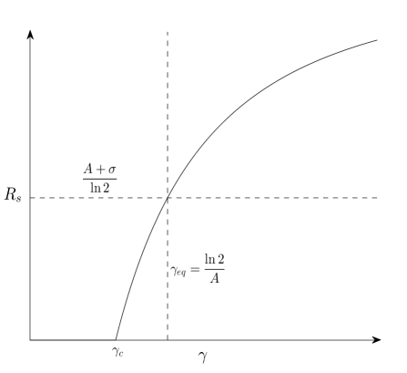
Figure 3: Illustration of the phase transition behavior in (23). $R_{s}$ is measured in $\mbox{bits}/\mbox{sec}$, and $\gamma$ is measured in sec. The plot is valid for a generic system and design parameters. In this specific example, we have chosen $A=5$, $\sigma=3$, and $\rho_{0}=0.7$. Consequently, $(A+\sigma)/\ln 2=11.5416$, $\ln 2/A=0.1386$, and $\gamma_{c}=0.0864$.

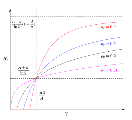
Figure 4: Illustration of the phase transition behavior in (23) for different values of $\rho_{0}$. $R_{s}$ is measured in $\mbox{bits}/\mbox{sec}$, and $\gamma$ is measured in sec. The plots are valid for a generic system and design parameters. In this specific example, we have chosen $A=1$, and $\sigma=0.5$. Therefore, $(A+\sigma)/\ln 2=2.1640$, $\ln 2/A=0.6931$, $\frac{A+\sigma}{\ln 2}(1+\frac{A}{\sigma})=6.4921$.

We make the following observations. For small values of $\gamma$, the amount of timing information carried by the triggering events is higher than what is needed to stabilize the system and the value of $R_{s}$ is zero. This means that if the delay is sufficiently small, then only a positive transmission rate is required to track the state of the system and the controller can successfully stabilize the system by receiving a single bit of information at every triggering event. This situation persists until a critical value $\gamma=\gamma_{c}$ is reached. This critical value is the solution of the equation

$$e^{A\gamma}-\rho_{0}e^{-\sigma\gamma}=1.$$

For this level of delay, the timing information of the triggering events becomes so much out of date that the transmission rate must begin to increase.

When $\gamma$ reaches the equilibrium point $\gamma_{eq}=\ln 2/A$, which equals the inverse of the intrinsic entropy rate of the system, the timing information carried by the triggering events compensates exactly the loss of information due to the delay introduced by the communication channel. This situation is analogous to having no delay, but also no timing information. It follows that in this case the required transmission rate matches the access rate in Theorem 1, and we have $R_{s}=(A+\sigma)/\ln 2$.

When $\gamma$ is increased even further, then the timing information carried by event triggering is excessively out of date and cannot fully compensate for the channel’s delay. The required transmission rate then exceeds the access rate imposed by the data-rate theorem. In this case, a more precise estimate of the state must be sent at every triggering time to compensate for the larger delay. Another interpretation of this behavior follows by considering the definition $H_{\rho(t_{s})}$ in (IV-A). The value $\gamma=\gamma_{eq}=\ln 2/A$ marks a transition point for $H_{\rho(t_{s})}$ from negative to positive values. For $\gamma>\gamma_{eq}$ event triggering does not supply enough information and $H_{\rho(t_{s})}$ presents a positive information balance in terms of the number of bits required to cover the uncertainty set. On the other hand, for $\gamma<\gamma_{eq}$, event triggering supplies more than enough information, and $H_{\rho(t_{s})}$ presents a negative information balance. We can then think of event triggering as a “source” supplying information, the controller as a “sink” consuming information, and $H_{\rho(t_{s})}$ as measuring the balance between the two, indicating whether additional information is needed in terms of quantized observations sent through the channel.

Finally, Figure 4 illustrates the phase transition for different values of $\rho_{0}$. For $\gamma<\gamma_{eq}$, since according to (17) smaller values of $\rho_{0}$ imply fewer triggering events, it follows that curves associated to smaller values of $\rho_{0}$ must have larger transmission rates to compensate for the lack of timing information. On the other hand, for $\gamma>\gamma_{eq}$ the situation is reversed. The timing information carried by the triggering events is now completely exhausted by the delay, and the controller relies only on the state information contained in the quantized packets. Since, according to (14), smaller values of $\rho_{0}$ imply larger packets sent through the channel and, for each value of the delay, the information in the larger packets becomes out of date at a slower rate than that in the smaller packets, it follows that in this case curves associated to smaller values of $\rho_{0}$ correspond to smaller transmission rates. Finally, we observe that all curves have the same asymptotic behavior for large values of $\gamma$, which is independent of $\rho_{0}$. This occurs because as $\gamma$ increases, more information needs to be sent through the channel and also the triggering rate decreases. Taking both effects into account yields the asymptotic value of the transmission rate $\frac{A+\sigma}{\ln 2}(1+\frac{A}{\sigma})$.

Remark 4.

The value of $\gamma_{c}$ is a threshold distinguishing whether (22) is zero or strictly positive. This threshold tends to $\gamma_{eq}=\ln 2/A$ as $\sigma\rightarrow 0$ and $\rho_{0}\rightarrow 1$. This is consistent with the fact that in this case there is only an asymptotic convergence guarantee (not an exponential one), and when the delay upper bound $\gamma$ is at most the inverse of entropy rate of the system only a positive transmission rate is necessary for stabilization. $\bullet$

IV-C Sufficient condition on the transmission rate

We now determine a sufficient transmission rate for the exponential convergence of the state estimation error using the event-triggering strategy described in Section II-B.

In our strategy, we let the sensor send a packet consisting of the sign of $z(t_{s})$ and a quantized version of $t_{s}$ to the controller. Using the bound (2), and the decoded packet, the controller constructs $q(t_{s})$, a quantized version of $t_{s}$. The controller then estimates $z(t_{c})$ as follows

$$\bar{z}(t_{c})=\text{sign}(z(t_{s}))v(q(t_{s}))e^{A(t_{c}-q(t_{s}))}.$$ (24)

The next result provides a bound on the error in the time quantization that guarantees that the requirements of the design are satisfied.

Lemma 5.

Under the assumptions of Lemma 1, using (24), if

$$|t_{s}-q(t_{s})|\leq\frac{1}{A+\sigma}\ln(1+\rho_{0}e^{-(\sigma+A)\gamma})$$ (25)

then (7) holds.

Proof.

Using (24), it follows that

$$|z(t_{c})- \bar{z}(t_{c})|$$ (26)

$$=v(t_{s})e^{A(t_{c}-t_{s})}\left|1-\frac{v(q(t_{s}))}{v(t_{s})}e^{A(t_{s}-q(t_{s}))}\right|$$

$$=v(t_{s})e^{A(t_{c}-t_{s})}\left|1-\frac{v_{0}e^{-\sigma q(t_{s})}}{v_{0}e^{-\sigma t_{s}}}e^{A(t_{s}-q(t_{s}))}\right|$$

$$=v(t_{s})e^{A(t_{c}-t_{s})}\left|1-e^{(A+\sigma)(t_{s}-q(t_{s}))}\right|.$$

As a consequence, (7) may be expressed as

$$|1-e^{(A+\sigma)(t_{s}-q(t_{s}))}|\leq\rho_{0}e^{-\sigma\gamma}e^{-A(t_{c}-t_{s})}.$$

The smallest possible value of $e^{-A(t_{c}-t_{s})}$ for $(t_{c}-t_{s})\in[0,\gamma]$ is $e^{-A\gamma}$. Therefore, by ensuring

$$\left|1-e^{(A+\sigma)(t_{s}-q(t_{s}))}\right|\leq\rho_{0}e^{-(\sigma+A)\gamma},$$ (27)

we can also ensure (7). The condition in  (27) can be rewritten as

$$1-\rho_{0}e^{-(\sigma+A)\gamma}\leq e^{(A+\sigma)(t_{s}-q(t_{s}))}\leq 1+\rho_{0}e^{-(\sigma+A)\gamma}.$$

Taking logarithms and dividing by $(A+\sigma)$, we obtain

$$\frac{1}{A+\sigma}\ln(1-x^{\prime})\leq t_{s}-q(t_{s})\leq\frac{1}{A+\sigma}\ln(1+x^{\prime}),$$ (28)

where $x^{\prime}=\rho_{0}e^{-(\sigma+A)\gamma}$. It follows that to satisfy (7) for all delay values it is enough that

$$|t_{s}-q(t_{s})|\leq\min\{|\frac{1}{A+\sigma}\ln(1-x^{\prime})|,|\frac{1}{A+\sigma}\ln(1+x^{\prime})|\}.$$

The result now follows. ∎

The next result presents a sufficient transmission rate, along with the design that meets it.

Theorem 3.

Under the assumptions of Lemma 1, if the state estimation error satisfies $|z(0)|<v_{0}$, then for any information transmission rate

$$R_{s}\geq\frac{A+\sigma}{-\ln(\rho_{0}e^{-\sigma\gamma})}\max\left\{0,1+\log\frac{b\gamma(A+\sigma)}{\ln(1+\rho_{0}e^{-(\sigma+A)\gamma})}\right\},$$ (29)

where $b>1$, there exists a quantization policy that achieves (7) for all $k\in\mathbb{N}$ (and consequently $|z(t)|\leq v_{0}e^{(A+\sigma)\gamma}e^{-\sigma t}$).

Proof.

Our proof strategy is as follows. We design a quantizer to construct a packet of length $g(t_{s})$ that the sensor sends to the controller. Using this packet, the decoder reconstructs the quantized version $q(t_{s})$ of $t_{s}$ satisfying (25). The result then follows from Lemma 5 and quantifying the associated transmission rate.

In our construction, the first bit of the packet determines the sign of $z(t_{s})$, i.e., whether $z(t_{s})=+v(t_{s})$ or $z(t_{s})=-v(t_{s})$. For quantizing $t_{s}$, we first divide the whole positive time line in sub-intervals of length $b\gamma$. Recall that the controller receives a packet at time $t_{c}$, and $t_{s}\in[t_{c}-\gamma,t_{c}]$. Noting that $b\gamma>\gamma$, upon the reception of the packet at time $t_{c}$ the decoder identifies two consecutive sub-intervals of length $b\gamma$ that $t_{s}$ can belong to — the second bit of the packet is $\text{mod}\left(\lfloor\frac{t_{s}}{b\gamma}\rfloor,2\right)$, which informs the decoder that $t_{s}\in[\iota b\gamma,(\iota+1)b\gamma]$ for some fixed $\iota$. The encoder divides this interval uniformly into $2^{g(t_{s})-2}$ sub-intervals, one of which contains $t_{s}$. After receiving the packet, the decoder determines the correct sub-interval and chooses $q(t_{s})$ as the middle point of it. With this strategy, we have

$$|t_{s}-q(t_{s})|\leq\frac{b\gamma}{2^{g(t_{s})-1}}.$$ (30)

Hence, from Lemma 5, it is enough to ensure

$$\frac{b\gamma}{2^{g(t_{s})-1}}\leq\frac{1}{A+\sigma}\ln(1+\rho_{0}e^{-(\sigma+A)\gamma}),$$ (31)

to guarantee that (7) holds. This is equivalent to

$$g(t_{s})\geq\max\left\{0,1+\log\frac{b\gamma(A+\sigma)}{\ln(1+\rho_{0}e^{-(\sigma+A)\gamma})}\right\}.$$ (32)

The characterization (29) of the transmission rate now follows from using this bound and the uniform upper bound on the triggering rate (17). ∎

Theorem 3 ensures the exponential convergence of the state estimation error. The following result shows that (29) is sufficient for asymptotic stabilizability when employing a linear controller.

Corollary 1.

Under the assumptions of Theorem 3, (29) is also a sufficient condition for asymptotic stabilizability.

Proof.

With $u(t)=-K\hat{x}(t)$, we can rewrite (1) as

$$\dot{x}(t)=(A-BK)x(t)+BKz(t).$$

As a consequence, we have

$$x(t)=e^{(A-BK)t}x(0)+e^{(A-BK)t}\int_{0}^{t}e^{-(A-BK)\tau}BKz(\tau)d\tau.$$

According to Theorem 3, (29) is sufficient to guarantee $\lim_{t\rightarrow\infty}z(t)=0$. Since $B\neq 0$ one can choose $K$ such that $A-BK<0$, and it follows that criterion (29) is also sufficient for $\lim_{t\rightarrow\infty}x(t)=0$. Stability can also be guaranteed from the above expression. ∎

It should be clear that if the quantization policy designed for establishing Theorem 3 satisfies Assumption 1, then the number of bits transmitted at each triggering time is finite. We conclude this section by providing a condition under which the designed policy satisfies Assumption 1.

Theorem 4.

Under the assumptions of Lemma 1, let $\nu\geq 2$, and let the number of bits in each transmitted packet be a constant $g(t_{s}^{k})=g$. If $g$ satisfies the lower bound (32) and the upper bound

$$g\leq\log\frac{b\gamma(A+\sigma)}{\left|\ln\left(1-\frac{1}{(\nu-1)\left(2+\dfrac{1}{\rho_{0}e^{-\sigma\gamma}}\right)}\right)\right|},$$ (33)

and

$$\frac{1-e^{-(A+\sigma)\frac{\delta}{2}}}{1-e^{-(A+\sigma)\frac{\delta}{4}}}\geq e^{(A+\sigma)\frac{3\delta}{4}},$$ (34)

where $\delta=b\gamma/2^{g-2}$, then the quantization policy used in Theorem 3 satisfies Assumption 1 at every triggering time.

Proof.

The proof follows from the following two claims.

Claim (a): For all $k\in\mathbb{N}$, if $t_{s}^{k}$ satisfies

$$-\frac{\delta}{2}=-\frac{b\gamma}{2^{g-1}}\leq t_{s}^{k}-q(t_{s}^{k})\leq-\frac{b\gamma}{2^{g}}=-\frac{\delta}{4},$$ (35)

then there exists a delay $\Delta_{k}\leq\beta$ such that (20) is satisfied.

Claim (b): The sequence of transmission times $\{t_{s}^{k}\}$ is uniquely determined by the initial condition $z(0)$ and there exists a $z(0)$ such that for each $k\in\mathbb{N}$, $t_{s}^{k}$ satisfies (35).

We first prove Claim (a). Note that when the sensor transmits $g$ bits, lower bounded by (32), the upper bound on the quantization error (30) holds and thus (35) is well defined. From (35) and (33), we have

$$t_{s}^{k}-q(t_{s}^{k})\leq\frac{1}{A+\sigma}\ln\left(1-\frac{1}{(\nu-1)(2+\frac{1}{\rho_{0}e^{-\sigma\gamma}})}\right),$$ (36)

where we have used the fact that $\nu\geq 2$ to simplify the absolute value. We rewrite this inequality as

$$1-e^{(A+\sigma)(t_{s}^{k}-q(t_{s}^{k}))} \geq\frac{\rho_{0}e^{-\sigma\gamma}}{(\nu-1)(1+2\rho_{0}e^{-\sigma\gamma})}>0.$$

Thus, from (26), we see that

$$|z(t_{c}^{k})-\bar{z}(t_{c}^{k})| \geq v(t_{s}^{k})e^{A\Delta_{k}}\frac{\rho_{0}e^{-\sigma\gamma}}{(\nu-1)(1+2\rho_{0}e^{-\sigma\gamma})}$$

$$\geq\frac{\rho(t_{s}^{k})}{\nu}e^{A(\Delta_{k}-\beta+\ln(\frac{\nu}{\nu-1}))}$$

$$\geq\frac{\rho(t_{s}^{k})}{\nu},\quad\forall\Delta_{k}\in\left[\beta-\ln\left(\frac{\nu}{\nu-1}\right),\beta\right],$$

where in the second inequality, we have used the definition of $\rho(t_{s}^{k})$ in (7). This proves Claim (a).

We now prove Claim (b). First, we need to determine the dependence of $t_{s}^{k+1}$ on $t_{s}^{k}$ and $\Delta_{k}$. Recall the triggering rule (5), which we express as $v(t_{s}^{k})e^{-\sigma\Delta^{\prime}_{k}}=|z(t_{c}^{k+})|e^{A(\Delta^{\prime}_{k}-\Delta_{k})}=v(t_{s}^{k})|1-e^{(A+\sigma)(t_{s}^{k}-q(t_{s}^{k}))}|e^{A\Delta^{\prime}_{k}}$, where we have used the fact $\Delta^{\prime}_{k}=t_{s}^{k+1}-t_{s}^{k}$ and (26). On simplification, we obtain

$$\Delta^{\prime}_{k}=\mathfrak{h}(t_{s}^{k}-q(t_{s}^{k})),$$ (37)

where, for convenience, we have defined $\mathfrak{h}(t):=-\frac{1}{A+\sigma}\ln(|1-e^{(A+\sigma)t}|)$. Notice that $t_{s}^{k+1}$ depends only on $t_{s}^{k}$ and not on $\Delta_{k}$ and. We show next that $t_{s}^{k}-q(t_{s}^{k})$ uniquely determines $t_{s}^{k+1}-q(t_{s}^{k+1})$.

To show this, recall that according to the proof of Theorem 3, the quantization policy has the encoder divide the interval $[\iota b\gamma,(\iota+1)b\gamma]$ for some fixed $\iota$ uniformly into $2^{g-2}$ sub-intervals, one of which includes $t_{s}^{k}$. The decoder chooses as $q(t_{s}^{k})$ the middle point of the sub-interval that contains $t_{s}^{k}$. Thus, we have

$$q(t)=\left\lfloor\frac{t}{\delta}\right\rfloor\delta+\frac{\delta}{2},\quad\delta=\frac{b\gamma}{2^{g-2}}.$$ (38)

Letting $y_{k}=t_{s}^{k}-q(t_{s}^{k})$, we obtain

$$y_{k+1} =t_{s}^{k}+\Delta^{\prime}_{k}-q(t_{s}^{k}+\Delta^{\prime}_{k})$$

$$=y_{k}+\left\lfloor\frac{t_{s}^{k}}{\delta}\right\rfloor\delta+\Delta^{\prime}_{k}-\left\lfloor\frac{y_{k}+\left\lfloor\frac{t_{s}^{k}}{\delta}\right\rfloor\delta+\frac{\delta}{2}+\Delta^{\prime}_{k}}{\delta}\right\rfloor\delta$$

$$=y_{k}+\mathfrak{h}(y_{k})-\left\lfloor\frac{y_{k}+\frac{\delta}{2}+\mathfrak{h}(y_{k})}{\delta}\right\rfloor\delta=:\mathcal{H}(y_{k}),$$

where in the second step we have used $t_{s}^{k}=y_{k}+q(t_{s}^{k})$ and (38), and in the third step we have used (37). From the conditions on $g$, we know that (30) is satisfied and hence $\mathcal{H}$ is a map from the interval $[-\frac{\delta}{2},\frac{\delta}{2}]$ onto itself. We also notice that $\mathcal{H}$ is a piecewise continuous function. In fact, it is easy to verify that on $[-\frac{\delta}{2},0)$, the function is piecewise strictly increasing. Further, note that if $\mathcal{H}$ is discontinuous at $w<0$, then the left limit of $\mathcal{H}$ at $w$ is $\delta/2$ while the right limit of $\mathcal{H}$ at $w$ is $-\delta/2$.

Next, (34) implies that

$$\ln(1-e^{-(A+\sigma)\frac{\delta}{2}})-\ln(1-e^{-(A+\sigma)\frac{\delta}{4}})\geq(A+\sigma)\frac{3\delta}{4},$$

which, after rearranging the terms, we see that it implies

$$-\frac{\delta}{4}+\mathfrak{h}\left(-\frac{\delta}{4}\right)\geq-\frac{\delta}{2}+\mathfrak{h}\left(-\frac{\delta}{2}\right)+\delta.$$

Now, observe that if $w_{1},w_{2}\in[-\frac{\delta}{2},\frac{\delta}{2}]$ are such that $w_{2}+\mathfrak{h}(w_{2})=w_{1}+\mathfrak{h}(w_{1})+n\delta$ for some $n\in\mathbb{Z}$, then $\mathcal{H}(w_{1})=\mathcal{H}(w_{2})$. As a result, we conclude that there exists an interval $I\in[-\frac{\delta}{2},-\frac{\delta}{4}]$ such that the restriction $\mathcal{H}:I\rightarrow[-\frac{\delta}{2},\frac{\delta}{2}]$ is continuous, one-to-one and onto. Hence the inverse mapping of this restriction is continuous and is a contraction and hence using the Banach contraction principle [51], there exists a fixed point of the original map $\mathcal{H}$ in $I$. Finally, note that as we sweep $z(0)$ through $(0,v(0)]$, $t_{s}^{1}$ varies continuously from $\infty$ to $0$. Thus, there exists a $z(0)$ such that $y_{1}=t_{s}^{1}-q(t_{s}^{1})$ is the fixed point in $I$. This proves Claim (b). ∎

Remark 5.

We use the assumption in (34) in the proof of Theorem 4 to be able to apply the Banach contraction principle in establishing the existence of a suitable initial condition. We use the assumption $\nu\geq 2$ to ensure that the upper bound in (33) is well defined. $\bullet$

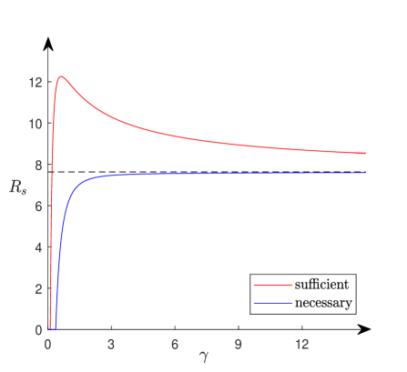
Figure 5: Comparison between the sufficient and necessary conditions. $R_{s}$ is measured in $\mbox{bits}/\mbox{sec}$, and $\gamma$ is measure in sec. Here, $A=1.3$, $\sigma=1$, $b=1.0001$, and $\rho_{0}=0.9$. The dashed line represents the asymptote $((A+\sigma)/\ln 2)(1+A/\sigma)=7.6319$.

Remark 6.

Figure 5 illustrates the gap between the sufficient conditiont (29) and the supremum over $\sigma$ of the necessary condition (22). For small values of $\gamma$, both conditions reduce to $R_{s}>0$. As $\gamma$ grows to infinity, both conditions converge to the same asymptote with value $\frac{A+\sigma}{\ln 2}(1+\frac{A}{\sigma})$. While (23) reaches the asymptote monotonically increasing for all $\rho_{0}$ values, the sufficient condition has an overshoot behavior for larger values of $\rho_{0}$ as depicted in Figure 6. For intermediate values of $\gamma$, the gap can be explained noticing that the exact value of the communication delay is unknown to the sensor and the controller, and hence there can be a mismatch between the uncertainty sets at the controller and the sensor. In addition, the sensor and the controller lack a common reference frame for the quantization of the transmission time. $\bullet$

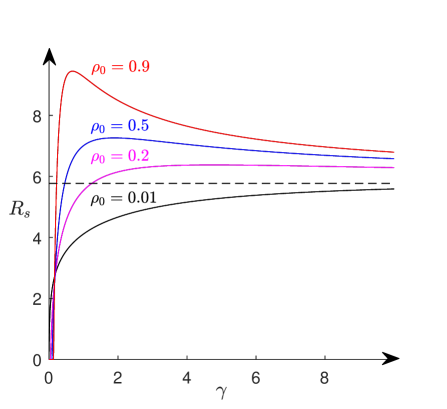
Figure 6: Illustration of the sufficient transmission rate for asymptotic observability versus the upper bound of delay for different values of $\rho_{0}$. $R_{s}$ is measured in $\mbox{bits}/\mbox{sec}$, and $\gamma$ is measure in sec. Here, $A=1$, $\sigma=1$, and $b=1.0001$. The dashed line represents the asymptote n$((A+\sigma)/\ln 2)(1+A/\sigma)=5.7708$.

IV-D Simulation

In this section, we illustrate an execution of our design for deriving the sufficient condition on the transmission rate. Using Theorem 3, we choose the size of the packet to be

$$g(t_{s})=\max\left\{1,\lceil 1+\log\frac{b\gamma(A+\sigma)}{\ln(1+\rho_{0}e^{-(\sigma+A)\gamma})}\rceil\right\},$$ (39)

where the ceiling operator ensures that the packet size is an integer number (we take the maximum between this quantity and 1 to make sure to send at least one bit  of data payload at each transmission).

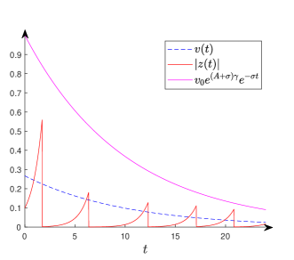
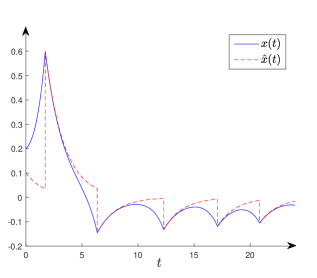
Figure 7: An example realization of our design. (a) shows the evolution of the absolute value of the state estimation error, the value of the event-triggering function, and the upper bound on the state estimation error. (b) shows the corresponding evolution of the state and state estimation. The continuous-time dynamics is discretized with step size $0.0002$. Because of this, a triggering happens when $z(t)$ becomes larger than the triggering function and there is no packet in the communication channel. In fact, since the sampling time is small, a triggering happens when $z(t)$ becomes approximately equal $v(t)$.

We illustrate the execution of our design for the system

$$\dot{x}(t)=x(t)+0.2u(t),\qquad u(t)=-8\hat{x}(t).$$

The event-triggering function is $v(t)=0.2671e^{-0.1t}$. The upper bound on the communication delay is $\gamma=1.2$. The design parameter are $b=1.0001$, $\rho_{0}=0.1$, and the initial condition $x(0)=0.2$, and $\hat{x}(0)=0.1$. Figure 7(a) shows the evolution of the state estimation error. The triggering strategy ensures that the state estimation error $z(t)$ converges exponentially to zero and triggering occurs every time the state estimation error crosses the triggering function $v(t)$. The overshoots observed in the plot are due to the unknown delay in the communication channel. Clearly, $|z(t)|$ is upper bounded by $v_{0}e^{(A+\sigma)\gamma}e^{-\sigma t}=e^{-0.1t}$. Figure 7(b) shows the corresponding evolution of $x(t)$ and $\hat{x}(t)$. The values of $x(t)$ and $\hat{x}(t)$ become close to each other at the reception times because of the jump strategy, while the distance between $x(t)$ and $\hat{x}(t)$ grows during the inter-reception interval.

Finally, Figure 8 shows the information transmission rate of a simulation versus the delay upper bound $\gamma$ in the channel. The packet size is chosen according to (39). We calculate the information transmission rate by multiplying the packet size and the number of triggering events in the simulation time interval divided by its length. One can observe from the plot that, for small delay upper bound $\gamma$, the system is stabilized with an information transmission rate smaller than the data-rate theorem ($3.75$ bits$/$sec in this example). Instead, for larger $\gamma$, the transmission rate becomes greater than the threshold determined by the data-rate theorem.

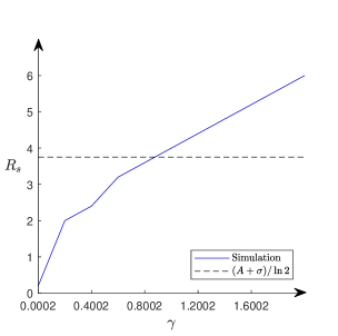
Figure 8: Information transmission rate versus the upper bound of the delay in the communication channel. $R_{s}$ is measured in $\mbox{bits}/\mbox{sec}$, and $\gamma$ is measured in sec. Here, $A=2.4$, $B=1$, $u(t)=-8\hat{x}(t)$, $\sigma=0.2$, $b=1.0001$, $\rho_{0}=0.1$, $v_{0}=0.0442$, $x(0)=0.201$, and $\hat{x}(0)=0.2$. The value of $\gamma$ ranges from $0.0005$ to $2.0005$, in steps of $0.2$. For each value of $\gamma$, we compute the transmission rate over an interval of $7$ seconds of simulation.

V Extension to vector systems

We generalize here our results to vector systems, building on the scalar case. Consider the plant-sensor-channel-controller tuple in Figure 1, and let the plant dynamics be described by a continuous-time, linear time-invariant (LTI) system

$$\dot{x}=Ax(t)+Bu(t),$$ (40)

where $x(t)\in\mathbb{R}^{n}$ and $u(t)\in\mathbb{R}^{m}$ for $t\in[0,\infty)$ are the plant state and the control input, respectively. Here, $A\in M_{n,n}(\mathbb{R})$, $B\in M_{n,m}(\mathbb{R})$, and $\|x(0)\|<L$, where $L$ is known to both sensor and controller. We assume all the eigenvalues of $A$ are real. Without loss of generality, we also assume that they are positive (since stable modes do not need any actuation and we can disregard them). In this setting, the intrinsic entropy rate of the plant is

$$h_{v}=\frac{\operatorname*{\operatorname{Tr}}(A)}{\ln 2}=\frac{\sum_{i=1}^{n}\lambda_{i}}{\ln 2}.$$ (41)

Hence, to guarantee stability it is necessary for the controller to have access to state information at a rate

$$R_{c}\geq h_{v}.$$

Using the Jordan block decomposition [52], we can write the matrix $A\in M_{n,n}(\mathbb{R})$ as $\Phi\Psi\Phi^{-1}$, where $\Phi$ is a real-valued invertible matrix and $\Psi=\text{diag}[J_{1},\ldots,J_{q}]$, where each $J_{j}$ is a Jordan block corresponding to the real-valued eigenvalue $\lambda_{j}$ of $A$. We let $p_{j}$ indicate the order of each Jordan block. For simplicity of exposition, we assume from here on that $A$ is equal to its Jordan block decomposition, that is, $A=\text{diag}[J_{1},\ldots,J_{q}]$.

In the following, we deal with each state coordinate separately. This corresponds to treating the $n$-dimensional system as $n$ scalar, coupled systems. When a triggering occurs for one of the coordinates, the controller should be aware of which coordinate the received packet corresponds to. Accordingly, we assume there are $n$ parallel finite-rate digital communication channels between each coordinate of the system and the controller, each subject to unknown, bounded delay.

We use the same notation of Section II, but add subindex $i$ and superindex $j$ to specify the $i^{\text{th}}$ coordinate of the $j^{\text{th}}$ Jordan block. So, for instance, $\{t_{s,i}^{k,j}\}_{k\in\mathbb{N}}$, $\{t_{c,i}^{k,j}\}_{k\in\mathbb{N}}$, $g(t_{s,i}^{k,j})$ denote the sequences of transmission times, reception times, and number of bits that the sensor transmits at each triggering time. Similarly, the $k^{\text{th}}$ communication delay $\Delta_{k,i}^{j}$ and $k^{\text{th}}$ triggering interval ${\Delta^{\prime}}_{k,i}^{j}$ can be specified for each coordinate. The communication delays for all coordinates are uniformly upper-bounded by $\gamma$, a non-negative real number known to both the sensor and the controller. The transmission rate for each coordinate is then

$$R_{s,i}^{j}=\limsup_{N_{i}^{j}\rightarrow\infty}\frac{\sum_{k=1}^{N_{i}^{j}}g(t_{s,i}^{k,j})}{\sum_{k=1}^{N_{i}^{j}}\Delta^{\prime j}_{k,i}}.$$

Assuming $n$ parallel communication channels between the plant and the controller, each devoted to a coordinate separately, we have

$$R_{s}=\sum_{j=1}^{q}\sum_{i=1}^{p_{j}}R_{s,i}^{j}.$$

Using the same notation of Section II, when referring to a generic triggering or reception time, we omit the superscript $k$.

The controller maintains an estimate $\hat{x}$ of the state, which evolves according to

$$\dot{\hat{x}}(t)=A\hat{x}(t)+Bu(t),$$ (42)

during the inter-reception times. The state estimation error is $z(t)=x(t)-\hat{x}(t)$, which initially is set to $z(0)=x(0)-x_{0}$. For the $i^{\text{th}}$ coordinate of the $j^{\text{th}}$ Jordan block, we consider an event-triggering function as in (4) with different initial values $v^{j}_{0}$ for each coordinate, namely

$$v_{i}^{j}(t)=v_{0,i}^{j}e^{-\sigma t}.$$ (43)

For each coordinate, we employ the triggering rule (5) and the jump strategy (6). When a triggering occurs for the $i^{\text{th}}$ coordinate of the $j^{\text{th}}$ Jordan block, we assume that the sensor sends a packet large enough to ensure

$$|z_{i}^{j}(t_{c,i}^{j+})|\leq\rho_{0}e^{-\sigma\gamma}v(t_{s,i}^{j}).$$ (44)

When referring to a generic Jordan block, we omit the superscript and subscript $j$.

Although each Jordan block is effectively independent of each other, the vector case is not an immediate extension of the scalar one. Specifically, from (40) and (42), we have that

$$\dot{z}_{1}(t) =\lambda z_{1}(t)+z_{2}(t)$$ (45)

$$\;\vdots$$

$$\dot{z}_{p-1}(t) =\lambda z_{p-1}(t)+z_{p}(t)$$

$$\dot{z}_{p}(t) =\lambda z_{p}(t),$$

where $p$ denotes the order of the Jordan block. This shows that the evolution of the coordinates is coupled and hence, even assuming parallel communication channels, care must be taken in generalizing the results for the scalar case.

Our first result generalizes Theorem 1 on the necessary condition for the information access rate.

Theorem 5.

Consider the plant-sensor-channel-controller model described in Section II, with plant dynamics (40), and state estimation error $z(t)$. Let $\sigma\in\mathbb{R}$ be positive, then the following necessary conditions hold:

1. If the state estimation error satisfies

   $$\|z(t)\|\leq\|z(0)\|~{}e^{-\sigma t},$$

   then

   $$b_{c}(t)\geq t~{}\frac{\operatorname*{\operatorname{Tr}}(A)+n\sigma}{\ln 2}+n~{}\log\frac{L}{\|z(0)\|}.$$

2. If the system in (40) is stabilizable and

   $$\|x(t)\|\leq\|x(0)\|~{}e^{-\sigma t},$$

   then

   $$b_{c}(t)\geq t~{}\frac{\operatorname*{\operatorname{Tr}}(A)+n\sigma}{\ln 2}.$$

In both cases, the information access rate is $R_{c}\geq\frac{\operatorname*{\operatorname{Tr}}(A)+n\sigma}{\ln 2}$.

The proof of this result, omitted for space reasons, is analogous to that of Theorem 1, noting that for $A\in M_{n,n}(\mathbb{R})$ and $X\in\mathbb{R}^{n}$, $m(AX)=|\det(A)|m(X)$, $\det(e^{A})=e^{\operatorname*{\operatorname{Tr}}(A)}$, and that the Lebesgue measure of a sphere of radius $\epsilon$ in $\mathbb{R}^{n}$ is $k_{n}\epsilon^{n}$, where $k_{n}$ is a constant that changes with dimension.

We next generalize the necessary condition on the information transmission rate. If $A$ is diagonalizable, then the necessary and sufficient bit rate for the vector system is equal to the sum of the necessary and sufficient bit rates that we provide in Section IV for each coordinate of the system. We now generalize this idea to any matrix with real eigenvalues.

Theorem 6.

Consider the plant-sensor-channel-controller model with plant dynamics (40), where all eigenvalues of $A$ are real, estimator dynamics (42), event-triggering strategy (5), event-triggering function (43), and packet sizes such that $z_{i}^{j}(t_{c,i}^{k,j})$ is determined at the controller within a ball of radius $\rho(t_{s,i}^{k,j})=\rho_{0}e^{-\sigma\gamma}v(t_{s,i}^{k,j})$ with $\nu$-precision, ensuring (44) via the jump strategy (6) for all $k\in\mathbb{N}$, $i=1,\ldots,p_{j}$, and $j=1,\ldots,q$. Then, there exists a delay realization and initial condition, such that

$$R_{s}\geq\sum_{j=1}^{q}\frac{p_{j}(\lambda_{j}+\sigma)}{\ln\nu+\ln(2+\frac{e^{\sigma\gamma}}{\rho_{0}})}\max\left\{0,\log\frac{(e^{\lambda_{j}\gamma}-1)}{\rho_{0}e^{-\sigma\gamma}}\right\}.$$

Proof.

Since there is no coupling across different Jordan blocks in (40), the inherent entropy rate (41) is

$$h_{v}(A)=h_{v}(J_{1})+\cdots+h_{v}(J_{q}).$$

Therefore, it is enough to prove the result for one of the Jordan blocks. Let $J$ be a Jordan block of order $p$ with associated eigenvalue $\lambda$. Note that the part of the vector $z(t)$ which corresponds to $J$ is governed by (45). The solution of the first differential equation in (45) is

$$z_{1}(t)=e^{\lambda t}z_{1}(0)+e^{\lambda t}\int_{0}^{t}e^{-\lambda\tau}z_{2}(\tau)d\tau.$$

If for the first coordinate a triggering event occurs at time $t_{s,1}$, then $z_{1}(t_{c,1})$ belongs to the set

$$\Omega(z(t_{c,1})|t_{s,1})=\{y=y_{1}+y_{2}:y_{1}=\pm v_{1}(t_{s,1})e^{\lambda(t_{c,1}-t_{s,1})},$$

$$\hskip 30.1388pty_{2}=\int_{t_{s,1}}^{t_{c,1}}e^{\lambda(t_{c,1}-\tau)}z_{2}(\tau)d\tau;\;t_{c,1}\in[t_{s,1},t_{s,1}+\gamma],$$

$$\hskip 64.58313ptz_{2}(\tau)\in\zeta_{\tau}^{s,2}~{}~{}\text{for}~{}\tau\in[t_{s,1},t_{c,1}]\},$$

where $\zeta_{\tau}^{s,2}$ is the uncertainty set for $z_{2}(\tau)$ at the sensor. We define

$$Y_{1} =\{y_{1}:y_{1}=\pm v(t_{s,1})e^{\lambda(t_{c,1}-t_{s,1})},t_{c,1}\in[t_{s,1},t_{s,1}+\gamma]\},$$

which is the uncertainty set of $z_{1}(t_{c,1})$ given $t_{s,1}$ for the differential equation $\dot{z}_{1}=\lambda z_{1}$. By comparing the definitions of the sets $\Omega(z(t_{c,1})|t_{s,1})$ and $Y_{1}$, we have

$$m(\Omega(z(t_{c,1})|t_{s,1}))\geq m(Y_{1}).$$

Finally, we apply Lemmas 2 and 4 for each coordinate separately, so that the necessary bit rate for each must satisfy

$$R_{s,i}\geq\frac{\lambda+\sigma}{\ln\nu+\ln(2+\frac{e^{\sigma\gamma}}{\rho_{0}})}\max\left\{0,\log\frac{(e^{\lambda\gamma}-1)}{\rho_{0}e^{-\sigma\gamma}}\right\}$$

for $i=1,\ldots,p$. The result now follows. ∎

Note that, when $\rho_{0}\ll e^{\sigma\gamma}/\max\{2,\nu\}$, the result in Theorem 6 can be simplified to

$$R_{s}\geq\sum_{j=1}^{q}\frac{p_{j}(\lambda_{j}+\sigma)}{\ln 2}\max\left\{0,1+\frac{\log(e^{\lambda_{j}\gamma}-1)}{-\log(\rho_{0}e^{-\sigma\gamma})}\right\}.$$

Our next result generalizes the sufficient condition of Theorem 3 to vector systems.

Theorem 7.

Consider the plant-sensor-channel-controller model with plant dynamics (40), where all eigenvalues of $A$ are real, estimator dynamics (42), event-triggering strategy (5), and event-triggering function (43). For the $j^{\text{th}}$ Jordan block choose the following sequence of design parameters

$$0<\rho_{1}^{j}<\ldots<\rho_{p_{j}-1}^{j}<\rho_{p_{j}}^{j}=\rho_{0}<1.$$

If the state estimation error satisfies $|z_{i}^{j}(0)|\leq v_{0,i}^{j}$, then we can achieve (44) and

$$|z_{i}^{j}(t)|\leq v_{0,i}^{j}((\rho_{0}-\rho_{i}^{j})+e^{(\lambda_{j}+\sigma)\gamma})e^{-\sigma t}$$

for $i=1,\ldots,p_{j}$ and $j=1,\ldots,q$, with an information transmission rate, $R_{s}$, at least equal to

$$\sum_{j=1}^{j=q}\sum_{i=1}^{i=p_{j}}\frac{(\lambda_{j}+\sigma)}{-\ln(\rho_{0}e^{-\sigma\gamma})}\max\left(0,1+\log\frac{b\gamma(\lambda_{j}+\sigma)}{\ln(1+\rho_{i}^{j}e^{-(\sigma+\lambda_{j})\gamma})}\right),$$

where

$$0<v_{0,i}^{j}\leq\frac{v_{0,i-1}^{j}(\lambda_{j}+\sigma)(\rho_{0}-\rho_{i}^{j})}{((\rho_{0}-\rho_{i}^{j})+e^{(\lambda_{j}+\sigma)\gamma})(e^{(\lambda_{j}+\sigma)\gamma}-1)},$$ (46)

for $i=2,\ldots,p_{j}$ and $j=1,\ldots,q$, and $b>1$.

Proof.

It is enough to prove the result for one Jordan block. The solution of the last two equations in (45) is

$$z_{p-1}(t) =e^{\lambda t}z_{p-1}(0)+e^{\lambda t}\int_{0}^{t}e^{-\lambda\tau}z_{p}(\tau)d\tau,$$ (47)

$${z}_{p}(t) =e^{\lambda t}z_{p}(0).$$

The differential equation that governs $z_{p}(t)$ is similar to what we considered in Theorem 3. It follows that if the transmission rate for coordinate $p$ is lower bounded as (29) and $|z_{p}(0)|\leq v_{0,p}$, then we can ensure $|z_{p}(t)|\leq v_{0,p}e^{(\sigma+\lambda)\gamma}e^{-\lambda t}$.

Assume now that a triggering happens for coordinate $p-1$ at time $t_{s,p-1}$, namely $|z_{p-1}(t_{s,p-1})|=v(t_{s,p-1})$, and the controller receives the packet related to coordinate $p-1$ at time $t_{c,p-1}$. Then the uncertainty set for $z_{p-1}(t_{c,p-1})$ at the controller is

$$\Omega(z(t_{c,p-1})|t_{c,p-1})=\{w_{p-1}=w_{p-1}^{(1)}+w_{p-1}^{(2)}:\\ w_{p-1}^{(1)}=\pm v_{p-1}(\bar{t}_{r,p-1})e^{\lambda(t_{c,p-1}-\bar{t}_{r,p-1})},\\ w_{p-1}^{(2)}=\int_{\bar{t}_{r,p-1}}^{t_{c,p-1}}e^{\lambda(t_{c,p-1}-\tau)}z_{p}(\tau)d\tau;\\ \bar{t}_{r,p-1}\in[t_{c,p}-\gamma,t_{c,p-1}],\\ z_{p}(\tau)\in\zeta_{\tau}^{c,p}~{}\text{for}~{}\tau\in[\bar{t}_{r,p-1},t_{c,p-1}]\},$$ (48)

where $\zeta_{\tau}^{c,p}$ is the uncertainty set for $z_{p}(\tau)$ at the controller. Clearly, the measure of $\Omega(z(t_{c,p-1})|t_{c,p-1})$ is larger when $w_{p-1}^{(1)}$ and $w_{p-1}^{(2)}$ in (48) have the same sign. Hence, we can assume that $z_{p-1}(\bar{t}_{r,p-1})$ and $z_{p}(\tau)$ for $\tau\in[\bar{t}_{r,p-1},t_{c,p-1}]$ and $\bar{t}_{r,p-1}\in[t_{c,p-1}-\gamma,t_{c,p-1}]$ are positive. Define

$$W_{p-1}=\{w_{p-1}=w_{p-1}^{(1)}+w_{p-1}^{(2)}:\\ w_{p-1}^{(1)}=\pm v_{p-1}(\bar{t}_{r,p-1})e^{A(t_{c,p-1}-\bar{t}_{r,p-1})},\\ w_{p-1}^{(2)}=\int_{\bar{t}_{r,p-1}}^{t_{c,p-1}}e^{\lambda(t_{c,p-1}-\tau)}z_{p}(\tau)d\tau;\\ \bar{t}_{r,p-1}\in[t_{c,p}-\gamma,t_{c,p-1}],\\ |z_{p}(\tau)|\leq v_{0,p}e^{(\sigma+\lambda)\gamma}e^{-\sigma\tau}~{}\text{for}~{}\tau\in[\bar{t}_{r,p-1},t_{c,p-1}]\}.$$

Clearly, we have

$$m(\Omega(z(t_{c,p-1})|t_{c,p-1}))\leq m(W_{p-1}).$$ (49)

Hence, a sufficient condition for $W_{p-1}$ will also be a sufficient condition for $\Omega(z(t_{c,p-1})|t_{c,p-1})$. We note that $W_{p-1}$ is the Brunn-Minkowski sum of the following sets

$$W_{p-1}^{(1)} =\{w_{p-1}^{(1)}:w_{p-1}^{(1)}=\pm v_{p-1}(\bar{t}_{r,p-1})e^{A(t_{c,p-1}-\bar{t}_{r,p-1})},$$

$$~{}~{}~{}~{}~{}~{}~{}~{}~{}~{}~{}~{}~{}~{}~{}~{}~{}~{}~{}~{}~{}~{}~{}~{}~{}~{}~{}~{}~{}~{}~{}\bar{t}_{r,p-1}\in[t_{c,p}-\gamma,t_{c,p-1}]\}$$

$$W_{p-1}^{(2)} =\{w_{p-1}^{(2)}:w_{p-1}^{(2)}=\int_{\bar{t}_{r,p-1}}^{t_{c,p-1}}e^{\lambda(t_{c,p-1}-\tau)}z_{p}(\tau)d\tau;$$

$$~{}~{}~{}|z_{p}(\tau)|\leq v_{0,p}e^{(\sigma+\lambda)\gamma}e^{-\sigma\tau}~{}\text{for}~{}\tau\in[\bar{t}_{r,p-1},t_{c,p-1}],$$

$$~{}~{}~{}~{}~{}~{}~{}~{}~{}~{}~{}~{}~{}~{}~{}~{}~{}~{}~{}~{}~{}~{}~{}~{}~{}~{}~{}~{}~{}~{}~{}\bar{t}_{r,p-1}\in[t_{c,p}-\gamma,t_{c,p-1}]\}.$$

By the Brunn-Minkowski inequality [53], we have

$$m(W_{p-1})\geq m(W_{p-1}^{(1)})+m(W_{p-1}^{(2)}).$$ (50)

The operators in the definition of $W_{p-1}^{(1)}$ and $W_{p-1}^{(2)}$ are continuous and the operator in the definition of $W_{p-1}^{(2)}$ is integral. Hence, even if during the time interval $[\bar{t}_{r,p-1},t_{c,p-1}]$ the value of $z_{p}(\tau)$ jumps according to (6), $W_{p-1}^{(2)}$ remains a connected compact set. Therefore, $W_{p-1}^{(1)}$ and $W_{p-1}^{(2)}$ are closed intervals that are translation and dilation of each other. In this case, the inequality (50) is tight [54], and by (49) we have

$$m(\Omega(z(t_{c,p-1})|t_{c,p-1}))\leq m(W_{p-1}^{(1)})+m(W_{p-1}^{(2)}).$$ (51)

This allows us to deal with each coordinate, $p-1$ and $p$, separately as follows. If there is no coupling in the differential equation that governs $z_{p-1}(t)$, we have

$$\dot{z}_{p-1}(t)=\lambda z_{p-1}(t).$$

Using Theorem  3, and equation (51) with the rate

$$R_{s,p-1}\geq$$ (52)

$$\quad\frac{\lambda+\sigma}{-\ln(\rho_{p-1}e^{-\sigma\gamma})}\max\Big{\{}0,1+\log\frac{b\gamma(\lambda+\sigma)}{\ln(1+\rho_{p-1}e^{-(\sigma+\lambda)\gamma})}\Big{\}},$$

we can ensure

$$\Upsilon_{t_{c,p-1}^{+}}^{c}\leq\rho_{p-1}v_{p-1}(t_{c,p-1})+m(W_{p-1}^{(2)}),$$ (53)

where $\Upsilon_{t_{c,p-1}^{+}}^{c}$ is the uncertainty set for $z_{p-1}(t_{c,p-1}^{+})$ at the controller.

We now find an upper bound for $m(W_{p-1}^{(2)})$ as follows. Since, $R_{s,p}$ is lower bounded as (29), we can ensure $|z_{p}(t)|\leq v_{0,p}e^{(\sigma+\lambda)\gamma}e^{-\sigma t}$, and

$$m(W_{p-1}^{(2)}) =\int_{t_{c,p-1}-\gamma}^{t_{c,p-1}}e^{\lambda(t_{c,p-1}-\tau)}z_{p}(\tau)d\tau$$

$$\leq v_{0,p}e^{(\sigma+\lambda)\gamma}e^{\lambda t_{c,p-1}}\int_{t_{c,p-1}-\gamma}^{t_{c,p-1}}e^{-(\lambda+\sigma)\tau}d\tau$$

$$=\frac{v_{0,p}e^{(\sigma+\lambda)\gamma}e^{-\sigma t_{c,p-1}}}{\lambda+\sigma}(e^{(\lambda+\sigma)\gamma}-1).$$ (54)

From (46), we have

$$v_{0,p}\leq\frac{v_{0,p-1}(\lambda+\sigma)(\rho_{0}-\rho_{p-1})}{e^{(\lambda+\sigma)\gamma}(e^{(\lambda+\sigma)\gamma}-1)}.$$

Hence,

$$\frac{v_{0,p}e^{(\sigma+\lambda)\gamma}e^{-\sigma t_{c,p-1}}}{\lambda+\sigma}(e^{(\lambda+\sigma)\gamma}-1) \leq(\rho_{0}-\rho_{p-1})v_{0,p-1}e^{-\sigma t_{c,p-1}}$$

$$=(\rho_{0}-\rho_{p-1})v_{p-1}(t_{c,p-1}).$$

Consequently, from (V) we have

$$m(W_{p-1}^{(2)})\leq(\rho_{0}-\rho_{p-1})v_{p-1}(t).$$ (55)

Therefore, using (53) and (55) we have $m(\Upsilon_{t_{c,p-1}^{+}}^{c})\leq\rho_{0}v_{p-1}(t_{c,p-1})$ and $|z_{p-1}(t_{c}^{+})|\leq\rho_{0}v_{p-1}(t_{c,p-1})$. When $R_{s,p}$ is lower bounded as (29) and $R_{s,p-1}$ is lower bounded as (52), we can ensure

$$|z_{p-1}(t)|\leq((\rho_{0}-\rho_{p-1})+e^{(\lambda+\sigma)\gamma})v_{p-1}(t_{c,p-1})$$

because the solution of the differential equation that governs $z_{p-1}$ is given in (47), and using (55) we have

$$|z(t_{c,p-1})|\leq$$

$$v_{p-1}(t_{c,p-1}-\gamma)e^{\lambda\gamma}+(\rho_{0}-\rho_{p-1})v_{p-1}(t_{c,p-1})$$

$$=((\rho_{0}-\rho_{p-1})+e^{(\lambda+\sigma)\gamma})v_{p-1}(t_{c,p-1}).$$

With the same procedure we can find the sufficient rate $R_{s,i}$ for $i=p-2,\ldots,1$, and this concludes the proof. ∎

Remark 7.

In a Jordan block of order $p_{j}$, the inequality (46) provides an upper bound on the value of the triggering function for coordinate $i$ using the value of the triggering function for coordinate $i-1$, where $i=2,\ldots,p_{j}$. This is a natural consequence of the coupling among the coordinates in a Jordan block, cf. (45), which makes the error in coordinate $i$ affect the error in coordinates $1$ to $i-1$, for each $i=2,\ldots,p_{j}$. $\bullet$

Corollary 1 can be generalized, provided $(A,B)$ is stabilizable, using a linear control $u(t)=-K\hat{x}(t)$ with $A-BK$ Hurwitz. This is a consequence of Theorem 7 which guarantees that, using the stated communication rate, the state estimation error for each coordinate converges to zero exponentially fast.

Remark 8.

In our discussion, we have assumed that $\hat{x}(t)$ is known to both controller and sensor. Since the sensor has access to the state, using the system dynamics, it can deduce $u(t)$, and then obtain $\hat{x}(t)$, cf. [28]. Note that the controller design for our sufficient condition is linear $u(t)=-K\hat{x}(t)$, and thus the sensor can deduce $\hat{x}(t)$ assuming that $BK$ is invertible. Alternatively, the controller can directly signal the acknowledgment of the reception of the packet (and as a result $t_{c}^{k}$) to the sensor by applying a control input to the system that excites a specific frequency of the state each time a symbol has been received, and the sensor can construct $\hat{x}(t)$ at all time $t$ if it knows the decoding rule at the controller. On the other hand, assuming knowledge of $\hat{x}(t)$ at the sensor does not affect the generality of the necessary condition. $\bullet$

VI Conclusions

We have studied event-triggered control strategies for stabilization and exponential observability of linear plants in the presence of unknown bounded delay in the communication channel between the sensor and the controller. Our study has been centered on quantifying the value of the timing information implicit in the triggering events. We have identified a necessary and a sufficient condition on the transmission rate required to guarantee stabilizability and observability of the system for a given event triggering strategy. Our results reveal a phase transition behavior as a function of the maximum delay in the communication channel, where for small delays, a positive transmission rate ensures the control objective is met, while for large delays, the necessary transmission rate is larger than that of classical data-rate theorems with periodic communication and no delay. Future research will consider disturbances to the plant dynamics, additional errors in the communication channel not caused by quantization, extensions to the case when the communication delay is a function of thepacket size, replacing the Assumption $1$ with packet size constraints, and the study of other event-triggering strategies.

Mohammad Javad Khojasteh (S’14) did his undergraduate study at the Sharif University of Technology. He received two B.Sc. degrees in electrical engineering and pure mathematics in 2015. He received the M.Sc. degree in electrical and computer engineering at the University of California San Diego (UCSD), La Jolla, CA, in 2017. Currently, he is pursuing a Ph.D. degree in electrical and computer engineering at UCSD under the advice of prof. Franceschetti. His research interests include networked control systems, machine learning, and robotics.

Pavankumar Tallapragada received the B.E. degree in Instrumentation Engineering from SGGS Institute of Engineering $\&$ Technology, Nanded, India in 2005, M.Sc. (Engg.) degree in Instrumentation from the Indian Institute of Science, Bangalore, India in 2007 and the Ph.D. degree in Mechanical Engineering from the University of Maryland, College Park in 2013. He held a postdoctoral position at the University of California, San Diego during 2014 to 2017. He is currently an Assistant Professor in the Department of Electrical Engineering at the Indian Institute of Science, Bengaluru, India. His research interests include event-triggered control, networked control systems, distributed control and networked transportation systems.

Jorge Cortés (M’02-SM’06-F’14) received the Licenciatura degree in mathematics from Universidad de Zaragoza, Zaragoza, Spain, in 1997, and the Ph.D. degree in engineering mathematics from Universidad Carlos III de Madrid, Madrid, Spain, in 2001. He held postdoctoral positions with the University of Twente, Twente, The Netherlands, and the University of Illinois at Urbana-Champaign, Urbana, IL, USA. He was an Assistant Professor with the Department of Applied Mathematics and Statistics, University of California, Santa Cruz, CA, USA, from 2004 to 2007. He is currently a Professor in the Department of Mechanical and Aerospace Engineering, University of California, San Diego, CA, USA. He is the author of Geometric, Control and Numerical Aspects of Nonholonomic Systems (Springer-Verlag, 2002) and co-author (together with F. Bullo and S. Martínez) of Distributed Control of Robotic Networks (Princeton University Press, 2009). He has been an IEEE Control Systems Society Distinguished Lecturer (2010-2014) and is an elected member for 2018-2020 of the Board of Governors of the IEEE Control Systems Society. His current research interests include distributed control and optimization, network science, opportunistic state-triggered control and coordination, reasoning under uncertainty, and distributed decision making in power networks, robotics, and transportation.

Massimo Franceschetti (M’98-SM’11-F’18) received the Laurea degree (with highest honors) in computer engineering from the University of Naples, Naples, Italy, in 1997, the M.S. and Ph.D. degrees in electrical engineering from the California Institute of Technology, Pasadena, CA, in 1999, and 2003, respectively. He is Professor of Electrical and Computer Engineering at the University of California at San Diego (UCSD). Before joining UCSD, he was a postdoctoral scholar at the University of California at Berkeley for two years. He has held visiting positions at the Vrije Universiteit Amsterdam, the École Polytechnique Fédérale de Lausanne, and the University of Trento. His research interests are in physical and information-based foundations of communication and control systems. He is a co-author of the book “Random Networks for Communication” and author of “Wave Theory of Information,” both published by Cambridge University Press. Dr. Franceschetti served as Associate Editor for Communication Networks of the IEEE Transactions on Information Theory (2009-2012), as Associate Editor of the IEEE Transactions on Control of Network Systems (2013-2016), as Associate Editor for the IEEE Transactions on Network Science and Engineering (2014-2017), and as Guest Associate Editor of the IEEE Journal on Selected Areas in Communications (2008, 2009). He also served as general chair for the North American School of Information Theory (2015). He was awarded the C. H. Wilts Prize in 2003 for best doctoral thesis in electrical engineering at Caltech; the S.A. Schelkunoff Award in 2005 for best paper in the IEEE Transactions on Antennas and Propagation, a National Science Foundation (NSF) CAREER award in 2006, an Office of Naval Research (ONR) Young Investigator Award in 2007, the IEEE Communications Society Best Tutorial Paper Award in 2010, and the IEEE Control theory society Ruberti young researcher award in 2012. He has been elected fellow of the IEEE in 2018, and he was nominated a Guggenheim Fellow for natural sciences, engineering, in 2019.

References

- [1] M. J. Khojasteh, P. Tallapragada, J. Cortés, and M. Franceschetti, “The value of timing information in event-triggered control: The scalar case,” Allerton Conference on Communication, Control, and Computing, pp. 1165–1172, Sept. 2016.
- [2] ——, “Time-triggering versus event-triggering control over communication channels,” in IEEE Conference on Decision and Control, Melbourne, Australia, Dec 2017, pp. 5432–5437.
- [3] K.-D. Kim and P. R. Kumar, “Cyber-physical systems: A perspective at the centennial,” Proceedings of the IEEE, vol. 100 (Special Centennial Issue), pp. 1287–1308, 2012.
- [4] R. M. Murray, K. J. Astrom, S. P. Boyd, R. W. Brockett, and G. Stein, “Future directions in control in an information-rich world,” IEEE Control Systems, vol. 23, no. 2, pp. 20–33, 2003.
- [5] D. F. Delchamps, “Stabilizing a linear system with quantized state feedback,” IEEE Transactions on Automatic Control, vol. 35, no. 8, pp. 916–924, 1990.
- [6] W. S. Wong and R. W. Brockett, “Systems with finite communication bandwidth constraints. II. stabilization with limited information feedback,” IEEE Transactions on Automatic Control, vol. 44, no. 5, pp. 1049–1053, 1999.
- [7] J. Baillieul, “Feedback designs for controlling device arrays with communication channel bandwidth constraints,” in ARO Workshop on Smart Structures, Pennsylvania State Univ, 1999, pp. 16–18.
- [8] S. Tatikonda and S. Mitter, “Control under communication constraints,” IEEE Transactions on Automatic Control, vol. 49, no. 7, pp. 1056–1068, 2004.
- [9] G. N. Nair and R. J. Evans, “Stabilizability of stochastic linear systems with finite feedback data rates,” SIAM Journal on Control and Optimization, vol. 43, no. 2, pp. 413–436, 2004.
- [10] N. C. Martins, M. A. Dahleh, and N. Elia, “Feedback stabilization of uncertain systems in the presence of a direct link,” IEEE Transactions on Automatic Control, vol. 51, no. 3, pp. 438–447, 2006.
- [11] P. Minero, M. Franceschetti, S. Dey, and G. N. Nair, “Data rate theorem for stabilization over time-varying feedback channels,” IEEE Transactions on Automatic Control, vol. 54, no. 2, pp. 243–255, 2009.
- [12] P. Minero, L. Coviello, and M. Franceschetti, “Stabilization over Markov feedback channels: the general case,” IEEE Transactions on Automatic Control, vol. 58, no. 2, pp. 349–362, 2013.
- [13] R. T. Sukhavasi and B. Hassibi, “Linear time-invariant anytime codes for control over noisy channels,” IEEE Transactions on Automatic Control, vol. 61, no. 12, pp. 3826–3841, 2016.
- [14] R. H. Middleton, A. J. Rojas, J. S. Freudenberg, and J. H. Braslavsky, “Feedback stabilization over a first order moving average Gaussian noise channel,” IEEE Transactions on Automatic Control, vol. 54, no. 1, pp. 163–167, 2009.
- [15] E. Ardestanizadeh and M. Franceschetti, “Control-theoretic approach to communication with feedback,” IEEE Transactions on Automatic Control, vol. 57, no. 10, pp. 2576–2587, 2012.
- [16] J. Ding, Y. Peres, G. Ranade, and A. Zhai, “When multiplicative noise stymies control,” Annals of applied probability, 2018, to appear.
- [17] C. De Persis, “n-bit stabilization of n-dimensional nonlinear systems in feedforward form,” IEEE Transactions on Automatic Control, vol. 50, no. 3, pp. 299–311, 2005.
- [18] D. Liberzon, “Nonlinear control with limited information,” Communications in Information & Systems, vol. 9, no. 1, pp. 41–58, 2009.
- [19] G. N. Nair, R. J. Evans, I. M. Mareels, and W. Moran, “Topological feedback entropy and nonlinear stabilization,” IEEE Transactions on Automatic Control, vol. 49, no. 9, pp. 1585–1597, 2004.
- [20] S. Tatikonda, A. Sahai, and S. Mitter, “Stochastic linear control over a communication channel,” IEEE transactions on Automatic Control, vol. 49, no. 9, pp. 1549–1561, 2004.
- [21] V. Kostina and B. Hassibi, “Rate-cost tradeoffs in control,” in Allerton Conference on Communication, Control, and Computing. Monticello, IL: IEEE, 2016, pp. 1157–1164.
- [22] A. Khina, Y. Nakahira, Y. Su, and B. Hassibi, “Algorithms for optimal control with fixed-rate feedback,” in IEEE Conference on Decision and Control, Melbourne, Australia, Dec 2017, pp. 6015–6020.
- [23] Q. Ling and H. Lin, “Necessary and sufficient bit rate conditions to stabilize quantized Markov jump linear systems,” in American Control Conference, Baltimore, MD, 2010, pp. 236–240.
- [24] G. Ranade and A. Sahai, “Control capacity,” in Information Theory (ISIT), 2015 IEEE International Symposium on. IEEE, 2015, pp. 2221–2225.
- [25] G. N. Nair, S. Dey, and R. J. Evans, “Communication-limited stabilisability of jump Markov linear systems,” in 15th Int. Symp. Mathematical Theory of Networks and Systems, Notre Dame, IN, 2002.
- [26] D. Liberzon, “Finite data-rate feedback stabilization of switched and hybrid linear systems,” Automatica, vol. 50, no. 2, pp. 409–420, 2014.
- [27] G. Yang and D. Liberzon, “Finite data-rate stabilization of a switched linear system with unknown disturbance,” IFAC-PapersOnLine, vol. 49, no. 18, pp. 1085–1090, 2016.
- [28] A. Sahai and S. Mitter, “The necessity and sufficiency of anytime capacity for stabilization of a linear system over a noisy communication link. Part I: Scalar systems,” IEEE Transactions on Information Theory, vol. 52, no. 8, pp. 3369–3395, 2006.
- [29] A. S. Matveev and A. V. Savkin, Estimation and control over communication networks. Springer Science & Business Media, 2009.
- [30] P. Minero and M. Franceschetti, “Anytime capacity of a class of Markov channels,” IEEE Transactions on Automatic Control, vol. 62, no. 3, pp. 1356–1367, 2017.
- [31] G. Nair, “A non-stochastic information theory for communication and state estimation,” IEEE Transactions on Automatic Control, vol. 58, pp. 1497–1510, 2013.
- [32] M. Franceschetti and P. Minero, “Elements of information theory for networked control systems,” in Information and Control in Networks. Springer, 2014, pp. 3–37.
- [33] B. G. N. Nair, F. Fagnani, S. Zampieri, and R. J. Evans, “Feedback control under data rate constraints: An overview,” Proceedings of the IEEE, vol. 95, no. 1, pp. 108–137, 2007.
- [34] S. Yüksel and T. Başar, Stochastic Networked Control Systems: Stabilization and Optimization under Information Constraints. Springer Science & Business Media, 2013.
- [35] K. J. Astrom and B. M. Bernhardsson, “Comparison of riemann and lebesgue sampling for first order stochastic systems,” in IEEE Conference on Decision and Control, vol. 2, Las Vegas, Nevada, USA, 2002, pp. 2011–2016.
- [36] P. Tabuada, “Event-triggered real-time scheduling of stabilizing control tasks,” IEEE Transactions on Automatic Control, vol. 52, no. 9, pp. 1680–1685, 2007.
- [37] W. P. M. H. Heemels, K. H. Johansson, and P. Tabuada, “An introduction to event-triggered and self-triggered control,” in IEEE Conference on Decision and Control, Maui, HI, 2012, pp. 3270–3285.
- [38] P. Tallapragada and J. Cortés, “Event-triggered stabilization of linear systems under bounded bit rates,” IEEE Transactions on Automatic Control, vol. 61, no. 6, pp. 1575–1589, 2016.
- [39] E. Kofman and J. H. Braslavsky, “Level crossing sampling in feedback stabilization under data-rate constraints,” in IEEE Conference on Decision and Control, San Diego, CA, 2006, pp. 4423–4428.
- [40] Q. Ling, “Bit rate conditions to stabilize a continuous-time scalar linear system based on event triggering,” IEEE Transactions on Automatic Control, 2017, to appear.
- [41] J. Pearson, J. P. Hespanha, and D. Liberzon, “Control with minimal cost-per-symbol encoding and quasi-optimality of event-based encoders,” IEEE Transactions on Automatic Control, vol. 62, no. 5, pp. 2286–2301, 2017.
- [42] L. Li, X. Wang, and M. Lemmon, “Stabilizing bit-rates in quantized event triggered control systems,” in Proceedings of the 15th ACM international conference on Hybrid Systems: Computation and Control. ACM, 2012, pp. 245–254.
- [43] ——, “Stabilizing bit-rate of disturbed event triggered control systems,” IFAC Proceedings Volumes, vol. 45, no. 9, pp. 70–75, 2012.
- [44] D. E. Quevedo, V. Gupta, W.-J. Ma, and S. Yüksel, “Stochastic stability of event-triggered anytime control,” IEEE Transactions on Automatic Control, vol. 59, no. 12, pp. 3373–3379, 2014.
- [45] B. Demirel, V. Gupta, and M. Johansson, “On the trade-off between control performance and communication cost for event-triggered control over lossy networks,” in Control Conference (ECC), 2013 European. IEEE, 2013, pp. 1168–1174.
- [46] P. Tallapragada, M. Franceschetti, and J. Cortés, “Event-triggered second-moment stabilization of linear systems under packet drops,” IEEE Transactions on Automatic Control, vol. 63, no. 8, pp. 2374–2388, 2018.
- [47] S. Linsenmayer, R. Blind, and F. Allgöwer, “Delay-dependent data rate bounds for containability of scalar systems,” IFAC-PapersOnLine, vol. 50, no. 1, pp. 7875–7880, 2017.
- [48] J. Hespanha, A. Ortega, and L. Vasudevan, “Towards the control of linear systems with minimum bit-rate,” in Proc. 15th Int. Symp. on Mathematical Theory of Networks and Systems (MTNS), 2002.
- [49] D. Liberzon and S. Mitra, “Entropy and minimal data rates for state estimation and model detection,” in Proceedings of the 19th International Conference on Hybrid Systems: Computation and Control. ACM, 2016, pp. 247–256.
- [50] K. H. Johansson, M. Egerstedt, J. Lygeros, and S. Sastry, “On the regularization of zeno hybrid automata,” Systems & control letters, vol. 38, no. 3, pp. 141–150, 1999.
- [51] C. C. Pugh, Real mathematical analysis. Springer, 2002, vol. 2011.
- [52] V. V. Prasolov, Problems and theorems in linear algebra. American Mathematical Soc., 1994, vol. 134.
- [53] R. Gardner, “The Brunn-Minkowski inequality,” Bulletin of the American Mathematical Society, vol. 39, no. 3, pp. 355–405, 2002.
- [54] D. Klain, “On the equality conditions of the Brunn-Minkowski theorem,” Proceedings of the American Mathematical Society, vol. 139, no. 10, pp. 3719–3726, 2011.