On Ehrhart Polynomials of Lattice Triangles

Abstract.

The Ehrhart polynomial of a lattice polygon $P$ is completely determined by the pair $(b(P),i(P))$ where $b(P)$ equals the number of lattice points on the boundary and $i(P)$ equals the number of interior lattice points. All possible pairs $(b(P),i(P))$ are completely described by a theorem due to Scott. In this note, we describe the shape of the set of pairs $(b(T),i(T))$ for lattice triangles $T$ by finding infinitely many new Scott-type inequalities.

Figure 1. The points $(b(T),i(T))$ for lattice triangles $T$ together with the open cones $\sigma_{c}^{\circ}$.

1. Introduction

A lattice polygon $P\subseteq{\mathds{R}}^{2}$ is the two-dimensional convex hull of finitely many lattice points, i.e.,points in ${\mathds{Z}}^{2}$. Two lattice polygons are equivalent if they are mapped onto each other by an affine-linear automorphism of ${\mathds{R}}^{2}$ which maps ${\mathds{Z}}^{2}$ onto ${\mathds{Z}}^{2}$. Let $b=b(P)$ (resp. $i=i(P)$) be the number of lattice points contained in the boundary (resp. in the interior) of $P$.

Pick’s Theorem [Pic99] allows to compute the area $a(P)$ of a lattice polygon $P$ from $b(P)$ and $i(P)$:

(1) $$a(P)=i(P)+\frac{b(P)}{2}-1\text{.}$$

The Ehrhart polynomial of $P$ is given by $|(kP)\cap{\mathds{Z}}^{2}|=a(P)k^{2}+\frac{b(P)}{2}k+1$ (for $k\in{\mathds{Z}}_{\geq 0}$). We refer to the textbook [BR07]. Therefore, the study of Ehrhart polynomials of lattice polygons reduces to the study of the set ${\mathcal{P}}$ of tuples $(b(P),i(P))$ for lattice polygons $P$. In 1976 Scott showed the following result:

Theorem 1.1 (Scott).

For a lattice polygon $P$ with $i(P)\geq 1$ either $(b(P),i(P))=(9,1)$ or $b(P)\leq 2i(P)+6$ holds.

As described in [HS09], this implies a complete description of Ehrhart polynomials of lattice polygons:

$${\mathcal{P}}=\{(b,0)\,:\,b\in{\mathds{Z}}_{\geq 3}\}\cup\{(b,i)\,:\,3\leq b\leq 2i+6,\,1\leq i\}\cup\{(9,1)\}\text{.}$$

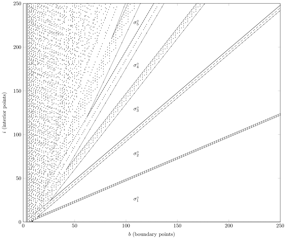
Figure 4. Zooming into Figure 1 for the values $0\leq b\leq 250$.

In this note, we investigate the subset ${\mathcal{T}}\subseteq{\mathcal{P}}$ of tuples $(b(T),i(T))$ for lattice triangles $T\subseteq{\mathds{R}}^{2}$. Since in Ehrhart theory results are often reduced to the case of lattice simplices, we are interested in understanding what this reduction means for the set of Ehrhart polynomials in the simplest case of dimension two. Rather surprisingly, it turns out that the structure of the set ${\mathcal{T}}$ is richer than one might have expected, as the reader can see in Figure 1 and Figure 4. While the structure of ${\mathcal{T}}$ is still to be fully understood, we explain here the appearance of the conspicuous “spikes”.

For this, let us introduce the following open affine cones (see Figure 1 and Figure 4).

Definition 1.2.

We set $\sigma_{c}^{\circ}\coloneqq\mathopen{}\mathclose{{}\left\{{(b,i)\in{\mathds{R}}_{\geq 0}^{2}\colon\tfrac{c-1}{2}b-(c-1)<i<\tfrac{c}{2}b-c(c+2)}}\right\}\subseteq{\mathds{R}}^{2}$ for $c\in{\mathds{Z}}_{\geq 1}$.

It is straightforward to check that the closures of these cones are pairwise disjoint. In this notation, Scott’s theorem (Theorem 1.1) is equivalent to the statement $\mathopen{}\mathclose{{}\left({\mathcal{P}}\setminus\{(9,1)\}}\right)\cap\sigma_{1}^{\circ}=\emptyset$. As suggested by Figure 1, the complement of ${\mathcal{T}}$ contains infinitely many more components.

Theorem 1.3.

We have ${\mathcal{T}}\cap\sigma_{c}^{\circ}=\emptyset$ for $c\in{\mathds{Z}}_{\geq 2}$.

For $c\in{\mathds{Z}}_{\geq 1}$ let $\widetilde{\sigma}_{c}$ be the translate of the closure of $\sigma^{\circ}_{c}$ so its apex is at the origin. As the cones $\widetilde{\sigma}_{c}$ cover the positive orthant, we see that there are no two-dimensional open affine cones in ${\mathds{R}}^{2}_{\geq 0}$ that are disjoint from all of the cones $\sigma_{c}^{\circ}$.

Remark 1.4.

1. There is a purely number-theoretic criterion to check whether a given pair $(b,i)$ is in ${\mathcal{T}}$. We have $(b,i)\in{\mathcal{T}}$ if and only if there exist integers $A,B,C\in{\mathds{Z}}$ with $A>0$ and $0\leq B<C$ such that $b=A+\gcd(B,C)+\gcd(B-A,C)$ and $i=(AC-b)/2+1$. In this case, the triangle with vertices $(0,0),(A,0),(B,C)$ can be chosen. These statements follow easily by considering Hermite normal forms (for details, see [Öbe15]).

2. Let us note that for $c\geq 1$, the apex of the closure of the cone $\sigma_{c}^{\circ}$ is $(2c^{2}+2c+2,c^{3}-c)\in{\mathcal{T}}$, realized by the lattice triangle with vertices $(0,0)$,$(2c^{2}+2c,0)$,$(1,c)$. Moreover, every pair $(b,i)\in{\mathds{Z}}^{2}$ on the lower facet of the closure of the cone $\sigma_{c}^{\circ}$ lies in ${\mathcal{T}}$ and is realized by the lattice triangle with vertices $(0,0)$,$\mathopen{}\mathclose{{}\left(\mathopen{}\mathclose{{}\left(2i+b-2}\right)/c,0}\right)$,$(B,c)$ for $B\in{\mathds{Z}}_{\geq 0}$ with $\gcd(B,c)=\gcd\mathopen{}\mathclose{{}\left(B-\mathopen{}\mathclose{{}\left(2i+b-2}\right)/c,c}\right)=1$. We also find infinitely many pairs $(k(c+1),kc(c+1)/2-c(c+2))\in{\mathcal{T}}$ (for $k\in{\mathds{Z}}_{\geq 2c+1}$) on the upper face of the closure of the cone $\sigma_{c}^{\circ}$, realized by the lattice triangles with vertices $(0,0)$,$((k-2)(c+1),0)$,$(0,c+1)$. These statements follow from elementary number-theoretic considerations.

3. The reader might notice many missing lines of slope $-1/2$ in Figure 4. The reason is that there are only two lattice triangles of prime normalized volume $2a$. More precisely, for odd primes $p$ we have ${\mathcal{T}}\cap\mathopen{}\mathclose{{}\left\{{i=-\tfrac{1}{2}b+\tfrac{p}{2}+1}}\right\}=\mathopen{}\mathclose{{}\left\{{(3,\tfrac{p-1}{2}),(p+2,0)}}\right\}$, for details see [Öbe15]. This follows also from Higashitani’s study of lattice simplices with prime normalized volume [Hig14].

4. From the pictures, it is visible that the points of ${\mathcal{T}}$ in the “spikes” form periodic patterns. It seems to be an interesting open question to make this observation precise.

5. Scott’s inequality (Theorem 1.1) follows from inequalities by del Pezzo and Jung [Jun90, DP87] (see also [Sch00]): any rational projective surface with degree $d$ and sectional genus $p>0$ satisfies $d\leq 4p+4$ if $(d,p)\not=(9,1)$. Now, Theorem 1.3 can be translated into algebraic geometry as follows: there exists no toric projective surface with Picard number one, degree $d$, and sectional genus $p$ that satisfies

   $$\tfrac{2(c+1)}{c}(c+p)<d<\tfrac{2c}{c-1}p$$

   for an integer $c\geq 2$. It would be interesting to see whether this is a special case of a more general algebro-geometric statement.

We remark that in an upcoming paper of the first author and Higashitani Theorem 1.3 will be used as the base case of a generalization for lattice simplices of dimension greater than two.

2. Proof of Theorem 1.3

Our proof uses the ideas of Scott’s original proof of Theorem 1.1. For the convenience of the reader we will give complete arguments without assuming prior knowledge of [Sco76]. Let $T$ be a lattice triangle with area $a$, number of boundary lattice points $b$, and number of interior lattice points $i$. We assume that $T$ satisfies for some $c\geq 2$ the inequalities

(2) $$c\mathopen{}\mathclose{{}\left(\tfrac{b}{2}-1}\right)<a<\tfrac{b}{2}(c+1)-(c+1)^{2}\text{.}$$

We will show that this situation cannot exist.

By replacing $T$ with an equivalent lattice triangle, we may assume that $T$ is contained in a bounding box (i.e.,a rectangle whose edges are parallel to the coordinate axes and that is minimal with respect to the inclusion of $T$) with vertical side length $p$ such that $p$ is minimal among all such choices. For an illustration, see Figure 2. Let us note that $p$ equals the lattice width of $T$. We denote the horizontal side length of the bounding box by $p^{\prime}$. We observe that necessarily $p^{\prime}\geq p$ since switching coordinates yields an equivalent triangle.

Figure 2. Two examples of bounding boxes used in the proof of Theorem 1.3.

Let us prove

(3) $$a\geq\tfrac{p^{2}}{4}$$

For this, we denote by $\delta$ the minimal distance of the $x$-coordinate of a vertex of $T$ (denoted by $\mathbf{v}_{2}$) on the top edge of the rectangle from the $x$-coordinate of a vertex of $T$ (denoted by $\mathbf{v}_{1}$) on the bottom edge of the rectangle. By an integral, unimodular shear leaving the horizontal line through the bottom edge of the rectangle invariant, we can achieve $\delta\leq\tfrac{p}{2}$. By possibly flipping along the horizontal or vertical axis, we may also assume that $\mathbf{v}_{2}$ has $x$-coordinate greater than or equal to that of $\mathbf{v}_{1}$, and the third vertex of $T$ (denoted by $\mathbf{v}_{3}$) has $x$-coordinate greater than or equal to that of $\mathbf{v}_{2}$ (recall that $p^{\prime}\geq p>\delta$).

Now, we move the bottom vertex $\mathbf{v}_{1}$ horizontally to the right until it has the same $x$-coordinate as that of $\mathbf{v}_{2}$. We observe that the area of the obtained triangle is bounded by the area of $T$ (see Figure 3), i.e.,

$$a\geq\tfrac{p(p^{\prime}-\delta)}{2}\geq\tfrac{p^{2}}{4}$$

where for the second inequality we used $\delta\leq\tfrac{p}{2}$ and $p^{\prime}\geq p$. This finishes the proof of (3).

$\quad\rightarrow\quad$

Figure 3. Illustration of the proof of inequality (3).

We may assume that there is only one vertex of $T$ on the top edge of the bounding box (otherwise, flip horizontally). Let us denote by $q$ the length of the intersection of $T$ with the bottom edge of the bounding box, so $q=0$ if and only if there is only one vertex of $T$ on the bottom edge.

As each horizontal line between $y=0$ and $y=p$ cuts the boundary of $T$ in two points (see Figure 2), we obtain

(4) $$b\leq q+2p\text{.}$$

We reformulate the inequality on the right hand side of (2) as

$$\tfrac{2a}{c+1}+2(c+1)<b\text{.}$$

By Pick’s Theorem (1), we have $a\in\tfrac{1}{2}{\mathds{N}}$, and thus the strict inequality becomes $\tfrac{2a+1+2(c+1)^{2}}{c+1}\leq b$. Combining this with (4) gives

(5) $$\tfrac{2a+1+2(c+1)^{2}}{c+1}\leq b\leq q+2p\text{.}$$

Let us assume $q=0$. Plugging in (3) yields

$$\tfrac{p^{2}/2+1+2(c+1)^{2}}{c+1}\leq 2p\Rightarrow p^{2}-4(c+1)p+2+4(c+1)^{2}\leq 0\text{.}$$

This is a contradiction as the discriminant of this quadratic polynomial in $p$ is negative.

Hence, $q>0$, so $a=\tfrac{pq}{2}$. Plugging this into (5) implies

$$\tfrac{pq+1+2(c+1)^{2}}{c+1}\leq q+2p\text{.}$$

Solving for $q$ yields

(6) $$(p-c-1)q\leq 2(c+1)(p-c-1)-1\text{.}$$

We see that $p\not=c+1$.

Let us assume $p<c+1$, i.e.,$p\leq c$. Clearly, $b\geq q+2$. We plug this in the inequality on the left hand side of (2) and get a contradiction, namely

$$\tfrac{cq}{2}<a=\tfrac{pq}{2}\leq\tfrac{cq}{2}\text{.}$$

Hence, we have $p>c+1$. We deduce from (6)

(7) $$q<2(c+1)\text{.}$$

Let us translate the left bottom vertex of $T$ into the origin. By applying an integral, unimodular shear leaving the horizontal line through the bottom edge of the rectangle invariant, we can get an equivalent triangle such that the $x$-coordinate of the top vertex of $T$ is in $[0,p)$. As $p^{\prime}\geq p$, this implies $q=p^{\prime}$, e.g., as in the left example of Figure 2.

The inequality on the left hand side of (2) is equivalent to $b<\tfrac{2a}{c}+2$. As $a=pq/2\in\tfrac{1}{2}{\mathds{N}}$, the strict inequality becomes

$$b\leq\tfrac{2a-1}{c}+2=\tfrac{pq-1}{c}+2\text{.}$$

Combining this with the inequality on the left hand side of (5), we obtain

$$\tfrac{pq+1+2(c+1)^{2}}{c+1}\leq b\leq\tfrac{pq-1}{c}+2\text{.}$$

Solving for $pq$ yields $2c(c^{2}+c+1)+1\leq pq$. As $q=p^{\prime}\geq p$ and $p>c+1$, the previous inequality combined with (7) implies

(8) $$2c(c^{2}+c+1)<pq\leq q^{2}<4(c+1)^{2}\Rightarrow 2c^{3}-2c^{2}-6c-4<0\text{.}$$

A straightforward computation shows that this is only possible for $c\leq 2$. As $c\geq 2$, we deduce $c=2$. Plugging this again into (8) we obtain $28<q^{2}<36$, a contradiction. ∎

References

- [BR07] Matthias Beck and Sinai Robins, Computing the continuous discretely, Undergraduate Texts in Mathematics, Springer, New York, 2007, Integer-point enumeration in polyhedra.
- [DP87] P Del Pezzo, On the surfaces of order n embedded in n-dimensional space, Rend. mat. Palermo 1 (1887), 241–271.
- [Hig14] Akihiro Higashitani, Ehrhart polynomials of integral simplices with prime volumes, Integers 14 (2014), Paper No. A45, 15.
- [HS09] Christian Haase and Josef Schicho, Lattice polygons and the number , Amer. Math. Monthly 116 (2009), no. 2, 151–165.
- [Jun90] G. Jung, Un’ osservazione sul grado massimo dei sistemi lineari di curve piane algebriche., Annali di Mat. (2) 18 (1890), 129–130.
- [Öbe15] Dennis Öberg, Ehrhart polynomials of lattice triangles, Bachelor thesis, Stockholm University, http://www.math.su.se/publikationer/uppsatsarkiv/tidigare-examensarbeten-i-matematik, 2015.
- [Pic99] Georg Pick, Geometrisches zur Zahlenlehre, Sitzungsber. Lotos (Prague) 19 (1899), 311–319.
- [Sch00] Josef Schicho, A degree bound for the parameterization of a rational surface, J. Pure Appl. Algebra 145 (2000), no. 1, 91–105.
- [Sco76] Paul R. Scott, On convex lattice polygons, Bull. Austral. Math. Soc. 15 (1976), no. 3, 395–399.