Probing shock geometry via the charge to mass ratio dependence of heavy ion spectra from multiple spacecraft observations of the 2013 November 4 event

Abstract

In large SEP events, ions can be accelerated at CME-driven shocks to very high energies. Spectra of heavy ions in many large SEP events show features such as roll-overs or spectral breaks. In some events when the spectra are plotted in energy/nucleon they can be shifted relative to each other to make the spectral breaks align. The amount of shift is charge-to-mass ratio (Q/A) dependent and varies from event to event. This can be understood if the spectra of heavy ions are organized by the diffusion coefficients (Cohen et al., 2005). In the work of Li et al. (2009), the Q/A dependences of the scaling is related to shock geometry when the CME-driven shock is close to the Sun. For events where multiple in-situ spacecraft observations exist, one may expect that different spacecraft are connected to different portions of the CME-driven shock that have different shock geometries, therefore yielding different Q/A dependence. In this work, we examine one SEP event which occurred on 2013 November 4. We study the Q/A dependence of the energy scaling for heavy ion spectra using Helium, oxygen and iron ions. Observations from STEREO-A, STEREO-B and ACE are examined. We find that the scalings are different for different spacecraft. We suggest that this is because ACE, STEREO-A and STEREO-B are connected to different parts of the shock that have different shock geometries. Our analysis indicates that studying the Q/A scaling of in-situ particle spectra can serve as a powerful tool to remotely examine the shock geometry for large SEP events.

1 Introduction

Understanding Solar Energetic Particles (SEPs) is a central topic of Space Plasma research. Studying SEPs provides a unique opportunity to examine the underlying particle acceleration process which exists at a variety of astrophysical sites. Furthermore, understanding SEPs is of practical importance since SEPs are a major concern of space weather. It is now widely accepted that these high energy particles are accelerated mostly at solar flares and shocks driven by coronal mass ejections (CMEs). Events where particles are accelerated mainly at flares are termed “impulsive” (Cane et al., 1986) as the time intensity profile shows a rapid rise and fast decay. In contrast, events where particles are accelerated mainly at CME-driven shocks are termed “gradual” (Cane et al., 1986; Reames, 1999) where the time intensity profiles vary gradually compared to impulsive events. For large SEP events, recent studies (e.g. Reames, 2009; Cliver, 2006; Gopalswamy et al., 2012; Mewaldt et al., 2012) suggested that energetic particles that are observed near Earth in these events are mostly accelerated at the shocks driven by CMEs rather than in flare active regions.

In many large SEP events, particle fluence spectra exhibit exponential rollover or double power law features (e.g. Mewaldt et al., 2005, 2012). The break energy or the roll-over energy, $E_{0}$, is between a few to a few 10’s of MeV/nucleon (Mazur et al., 1992; Cohen et al., 2005; Mewaldt et al., 2005; Tylka et al., 2005; Desai et al., 2016a). Simulations (Li, Zank & Rice, 2005) show that spectral breaks can occur naturally for particle acceleration at a CME-driven shock. In examining these features, Cohen et al. (2003, 2005) and Mewaldt et al. (2005) noted that the break energies are nicely ordered by $(Q/A)^{\sigma}$. They suggested that this ordering can be understood if the energy breaks or roll-overs for different heavy ions occur at the same values of the diffusion coefficient $\kappa$. Later, Li et al. (2009) attempted to relate $\sigma$ to shock geometry. They showed that the value of $\sigma$ is usually in the range of $1$ to $2$ for parallel shocks, but can become as small as $\sim 1/5$ for perpendicular shocks.

For the most general case of an oblique shock, the total diffusion coefficient is given by,

$$\kappa=\kappa_{||}\cos^{2}(\theta_{BN})+\kappa_{\perp}\sin^{2}(\theta_{BN}).$$ (1)

In the above, $\kappa_{||}$ and $\kappa_{\perp}$ are the parallel and perpendicular diffusion coefficients and $\theta_{BN}$ is the angle between the upstream magnetic field and the shock normal. Since in general $\kappa_{||}$ and $\kappa_{\perp}$ have different $Q/A$ dependence (Li et al., 2009), equation (1) yields a complicated $Q/A$ dependence for the break energy at an oblique shock. Recently, Desai et al. (2016a) have surveyed $0.1$-$100$ MeV/nucleon H-Fe fluence spectra for $46$ isolated large gradual SEP events observed at ACE during solar cycles 23 and 24. They found that the range of $\sigma$ for heavy ion spectra in these events is mostly between $0.2$ to $2$, although some events have a $\sigma$ value larger than $2$.

In the work of Li et al. (2009), it is assumed that the spectral break or roll-over from in-situ observations reflects the same feature of the escaped particle spectra at the shock. We note that some recent calculations have suggested that spectral breaks can emerge as a transport effect (Li & Lee, 2015; Zhao et al., 2016). However, in these calculations, the size of the spectral index change, i.e. $\delta\gamma=\gamma_{a}-\gamma_{b}$, where $\gamma_{a}$ and $\gamma_{b}$ are the spectral indices above and below the break energy $E_{0}$, is very small. This is in contrast to the observations where $\delta\gamma$ can be large and varies noticeably from one event to another. Furthermore, the transport effect shown in (Li & Lee, 2015; Zhao et al., 2016) predicts a $Q/A^{\sigma}$ dependence of the spectra break energy $E_{0}$ with an upper limit of $\sigma$ to be $1.3$. In a recent statistical suryey however, Desai et al. (2016b) found that $\sigma$ in $33$ SEP events ranged between $\sim 0.2-3$, which clearly exceeds the upper limit of $\sim 1.3$ predicted by scatter-dominated transport models (Li & Lee, 2015; Zhao et al., 2016).

Here we follow Li et al. (2009) and assume that the break is a feature of the escaped particle spectrum at the shock. Note that the Diffusive Shock Acceleration (DSA) does not predict a spectral break for the shock-accelerated particle spectrum. Nevertheless, there could be a variety of reasons for such a break. For example, the break may represent the maximum energy given a finite acceleration time. In this case we expect the break energies to be high, $>$ several $10$’s of MeVs for protons. It could also represent the cut-off energy for escape, i.e., particles with energy lower than the break energy are trapped more within the shock complex. In this case, the break energies may be low, $\sim<$ several MeV for protons. In both cases, however, the break energy is decided by the diffusion coefficient $\kappa$, so that the same $Q/A$ analysis discussed in the work of Li et al. (2009) applies.

Here we do not discuss the underlying mechanism that leads to the spectral break, but use the $Q/A$ scaling of heavy ion spectra to remotely infer the shock geometry. We note that since particles are continuously accelerated at the CME-driven shock, this shock geometry reflects only an ensemble average of the shock geometry over a period. If however, the energetic particles near the break energy are mostly accelerated at early times (i.e. in the case of the break energy representing the maximum energy), then we expect that the spectral break reflects the shock geometry when the shock is still close to the Sun.

Since for the same CME the shock geometry differs at different longitudes, then with simultaneous in-situ observations from multiple spacecraft, one may obtain different Q/A-scaling. This is illustrated in the cartoon shown in Figure 1. In the cartoon, the two field lines colored in blue (assumed here to be unperturbed Parker field) intersect with the shock at a quasi-perpendicular configuration and the two field lines colored in green intersect with the shock at a quasi-parallel configuration.

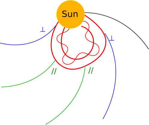
Figure 1: A cartoon showing that two spacecraft can be magnetically connected to different portions of a CME-driven shock which have different shock geometries.

The above discussion indicates that studying the Q/A scaling of heavy ion spectra simultaneously at multiple spacecraft may be used to infer shock geometry of the CME-driven shock for SEP events where heavy ion spectra are well organized by Q/A. In this work, we examine one such SEP event that occurred on 2013 November 4. In the following, we describe the observation in section 2 and present the fitting results in section 3. We conclude in section 4.

2 Observations

We study the SEP event using energetic particle measurements obtained by the Ultra-Low Energy Isotope Spectrometer (ULEIS) (Mason et al., 1998) and Solar Isotope Spectrometer (SIS) (Stone et al., 1998) on the Advanced Composition Explorer (ACE); and the Suprathermal Ion Telescope (SIT) (Mason et al., 2008) and Low Energy Telescope (LET) (Mewaldt et al., 2008) on the twin spacecraft Solar TErrestrial RElations Observatory (STEREO) A and B. On 2013 November 4 00:00 UT, the angle between ACE and STEREO-A (STA) was $148.56^{\circ}$, and the angle between ACE and STEREO-B (STB) was $143.24^{\circ}$. Panel (a) of Figure 2 shows the configuration of STA, STB and ACE for the event and the time intensity profiles of Helium for all three spacecraft. The eruption occurred on 2013 November 4 05:12:05 UT as identified from the CME catalog . The event is also included in the survey of Richardson et al. (2014). The event is a backside halo event as viewed from the Earth; a frontside and slightly western event as viewed from STA; and an eastern event from STB. Without X-ray observations, we do not know the flare class for this event. Panels e) and f) show the EUVI 171 observations from STA and STB. The active region (AR) is marked by the red circle.

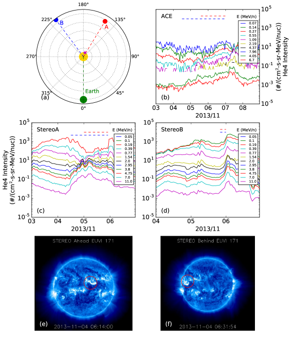
Figure 2: 2013 November 4 SEP event observed by three spacecraft. (a) locations of STA, Earth and STB at 2013 November 4 00:00 UT. (b) time intensity profiles of ⁴He observed by ACE from 2013 November 3 to November 8. (c) time intensity profiles of ⁴He observed by STA from 2013 November 3 to November 6. (d) time intensity profiles of ⁴He observed by STB from 2013 November 4 to November 6. (e) and (f) show the EUVI 171 observations of STA and STB. The active region is marked by the red circle.

Panels b), c) and d) of Figure 2 show the time intensity profiles of helium as observed by ACE, STA, and STB, respectively. The event was clearly seen at STA and STB. For ACE, even though it was a backside event, one can still see the gradual increase from the background. Note that another event from the same AR had occurred on 2013 November 2 (see Richardson et al. (2014)), and the SEPs from that event elevated the intensities at all three spacecraft.

The periods we choose for spectral analysis are shown by the dashed lines in panels b), c) and d). For STA and ACE, the elevated pre-event background makes it difficult to identify the onset times for the lower energy ions. We therefore use two different periods for different energies: the red dashed lines (November 5 00:00 UT to November 5 22:00 UT) indicate the time interval for the SIT instrument and the blue dashed lines (November 4 12:00 UT to November 5 22:00 UT) indicate the time interval for the LET instrument. Similarly for ACE we also use two different periods for different energies: the red dashed lines (November 5 14:00 UT to November 7 02:00 UT) indicates the time interval for the ULEIS instrument and the blue dashed lines (November 4 12:00 UT to November 7 02:00 UT) indicate the time interval for the SIS instrument. For STB, since this is an eastern event, clear increases of the time-intensity profiles do not occur until the end of November 5. So we choose November 5 20:00 UT to November 6 00:00 UT for all energy channels for STB. For STA and STB observations, we choose the stop time of the interval as the time at which the intensities peak. We do not include energetic particles in the downstream. One reason for doing so is that as shown in Zank et al. (2015), particles can be accelerated at magnetic islands downstream of a shock, leading to an extra acceleration in addition to the shock acceleration. This acceleration may have a different Q/A dependence. Furthermore, turbulence is often stronger downstream of a CME-driven shock and additional second-order Fermi acceleration may occur. Such an acceleration is also Q/A dependent. We therefore do not include downstream periods in our analysis. For the ACE observation, there was no local shock arrival since it was a backside event. We choose the stop time as November 7 00:00 UT, which is the onset time of a following event.

In obtaining the integrated energy spectra, we only include energy channels that show a clear increase from the background in the time intensity profiles. We do not subtract the pre-event background since the intensities were decaying from a previous event and the identification of a proper pre-event background is difficult. This should not introduce a large uncertainty since the pre-event backgrounds were well below the intensity levels during the chosen time periods.

The pre-event background does affect the time periods we select for obtaining the spectra. As we mentioned above, we use different time periods for STA/SIT and STA/LET observations. This is because, as shown in panel (c) of Figure 2, the intensities of lower energy Helium (below 2 MeV/nucleon) between November 4 12:00 UT and November 5 00:00 UT are still in the decay phase of the previous event. If we assume the intensities in these energy channels behave similarly to that of the $\sim 2-4$ MeV/nucleon channel, then using the $2-4$ MeV/nucleon intensity profile as a reference, we can normalize the time integrated intensities for the period denoted by the red dashed line to that denoted by the blue dashed line. In practice, by noting that for Helium and oxygen observations there is overlap between the LET energy channel of $4.25$ MeV/nucleon and the SIT energy channel of $4.37$ MeV/nucleon, we normalize the intensities of all LET energy channels by multiplying a factor ($1.8$) such that the integrated intensity of the LET $4.25$ MeV/nucleon equals that of the SIT energy channel of $4.37$ MeV/nucleon. This accounts for the different time intervals used for LET and SIT. We follow the same procedure for calculating the ACE spectra and use the energy channel of $4.37$ MeV/nucleon of ULEIS and $4.05$ MeV/nucleon of SIS for the normalization.

3 Results

We scale Fe and He spectra to match that of O. The scaling can be seen from the following condition:

$$\frac{(Q/A)^{\sigma}_{i}}{(Q/A)^{\sigma}_{O}}=\frac{E_{i}}{E_{O}}$$ (2)

where $i$ is He or Fe.

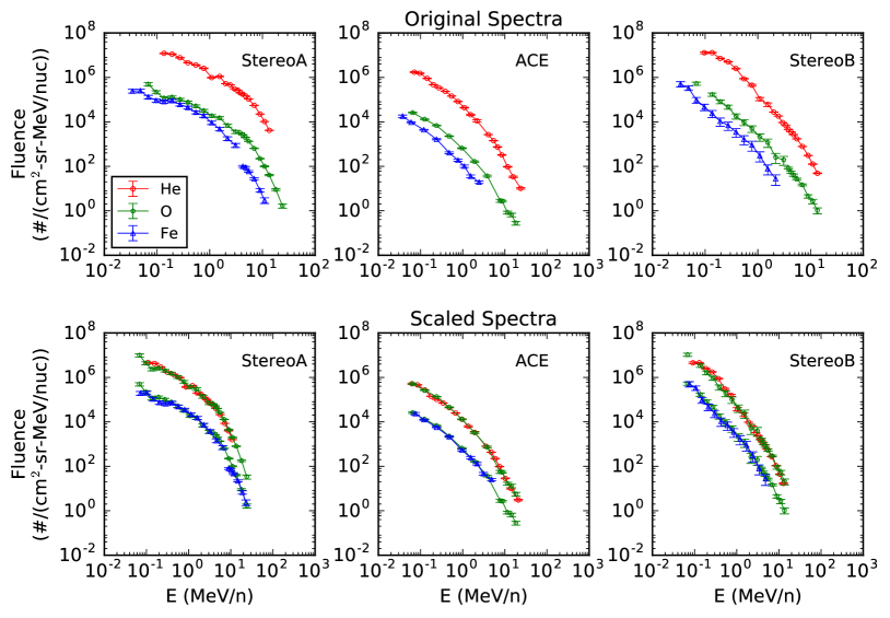
Figure 3: Spectra of Helium, oxygen and iron from STA, ACE, and STB, from the left to the right respectively. Upper panels are for the original spectra and lower panels are the scaled spectra. Energy spectra are shifted horizontally and vertically to make the comparison easier.

Figure 3 shows the original and the scaled time-integrated spectra. Statistical uncertainties are also shown. The upper panels are the original spectra and the lower panels are the spectra after scaling. In the scaled spectra, for better comparison, oxygen spectra are plotted twice, once shifted upward by a factor of $20$. The Fe spectra are shifted to the right and the He spectra are shifted to the left to match the “roll-over” features of the O spectra. The spectra of Fe and He are also shifted vertically to make the comparison easier. Statistical uncertainties are shown in the figure. In the following, however, the scaling factors only refer to the energy scaling (i.e. the horizontal shift). For STA observations, the energy scaling factor for iron is $2.1$, for Helium it is $0.80$. For STB observations, the energy scaling factor for iron is $1.6$, for Helium it is $0.95$. For ACE observations, the energy scaling factor for iron is $2.0$, for Helium it is $0.88$.

Assuming the charge state of Helium $Q_{He}=2$, we examine possible charge state of oxygen in the range of $Q_{O}=6$ to $7.9$. We increase $Q_{O}$ from $6$ with a step of $\delta Q=0.1$. For each $Q_{O}$ we obtain the corresponding $\sigma$ using equation (2) with $i=He$ and then using equation (2) again to obtain the charge state of iron $Q_{Fe}$ with $i=Fe$. The left panel of Figure 4 shows the value of $Q_{Fe}$ and $Q_{O}$ from our fitting. The red curve is for the STA observations, the blue curve is the STB observations and the green curve is for the ACE observations. The shaded area in the left panel represents the most probable charge states of oxygen from $6.0$ to $7.5$ and of iron from $10$ to $14$ (see discussions below). The right panel shows the corresponding $\sigma$ value.

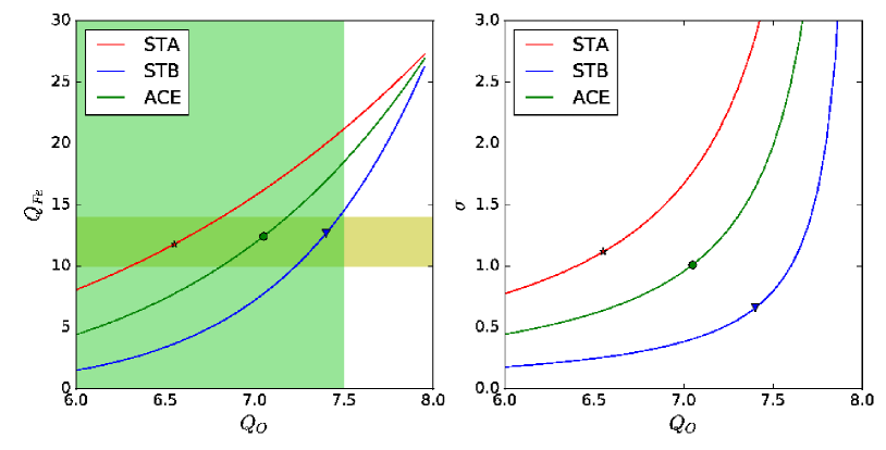
Figure 4: Left: charge state of Fe versus charge state of O. The shaded area represents the most probable charge state of O from $6.0$ to $7.5$ and of Fe from $10$ to $14$. Right: coefficient $\sigma$ versus charge state of O.

For STA (red curve), a charge state of oxygen from $6.0$ to $7.9$ yields a charge state of Fe from $8.1$ to $26.5$ and the corresponding $\sigma$ is from $0.8$ to $17.7$. For ACE (green curve), a charge state of oxygen from $6.0$ to $7.9$ yields a charge state of $4.4$ to $25.8$ for Fe and a corresponding $\sigma$ from $0.44$ to $10.2$. For STB (dark blue curve), a charge state of oxygen from $6.0$ to $7.9$ yields a charge state of $1.5$ to $24.6$ for Fe and a corresponding $\sigma$ from $0.18$ to $4.1$. Note that the range of $\sigma$ shown in Figure 4 is from $0$ to $3$, similar to that obtained in Desai et al. (2016a).

The charge states of O and Fe considered by Cohen et al. (2005) are $6.8$ and $11.6$, respectively. While the charge state for O can be from $6$ to $8$ for any given SEP event, that for Fe is mostly between $10.0$ to $14.0$ (e.g. Labrador et al., 2005; Mason et al., 2012). If we vary the charge state of iron $Q_{Fe}$ from $10.0$ to $14.0$, then from Equation 2 we find a charge state $Q_{O}=7.23$ to $7.47$, and $\sigma$ = $0.51$ to $0.74$ for STB; $Q_{O}=6.88$ to $7.22$, and $\sigma$ = $0.84$ to $1.24$ for ACE; $Q_{O}=6.31$ to $6.80$, and $\sigma$ = $0.94$ to $1.78$ for STA.

In Tylka & Lee (2006), the authors argue that the injection energy increases with shock obliquity, leading to a higher $Fe/O$ ratio and higher charge states at quasi-perpendicular shocks. These higher charge states may be from previous impulsive SEP material, which typically has greater energies than solar wind material (Tylka & Lee, 2006). Li et al. (2009) obtained a $\sigma\sim 0.22<1$ for a perpendicular shock. In our event, the STB observation yields a $\sigma<1$ and may correspond to a quasi-perpendicular portion of the shock. The STA observation has a $\sigma$ larger than $1$ for most charge states of iron we considered, and is consistent with a quasi-parallel shock. The ACE observations lie in between STB and STA. If we assume the charge states of both iron and oxygen increase with shock obliquity, and that STA (STB) connects to the quasi-parallel (quasi-perpendicular) part of the shock (while ACE connects to a portion of the shock having an obliquity in between STA’s and STB’s), then a possible choice of ($Q_{Fe}$, $Q_{O}$, $\sigma$) can be ($12.7$, $7.4$, $0.66$) for STB, ($12.4$, $7.0$, $1.01$) for ACE, and ($11.8$, $6.6$, $1.12$) for STA. We choose these values such that the values of $\sigma$ increase from STB to ACE and to STA. These choices are labeled as “star”, “circle” and “triangle” symbols in Figure 4. This is consistent with the cartoon shown in Figure 1 since STB saw an eastern event and STA saw a central event. For ACE, it is a backside event, the corresponding shock geometry is not clear from Figure 1. Comparing the charge state choices for STA and STB, we see that for both oxygen and iron, the charge states of STB observation is about $1$ unit larger than those of STA observations. This difference may reflect the injection and seed population dependence on shock geometry. We remark that direct charge state measurements for energetic particles from future missions such as IMAP will be helpful in resolving this dependence.

4 Discussion and Conclusion

In this paper, we examine the spectra of heavy ions of the 2013 November 4 SEP event from STA, STB, and ACE. We select this event because the time-integrated heavy ion spectra from all three spacecraft show spectral break features above $\sim 1$ Mev/nucleon. Although the pre-event background is elevated due to the presence of SEPs from another event that had occurred two days earlier, time intensity profiles from all three spacecraft show clear increases from the background. Our analyses show that: 1) for all three spacecraft the He, O, and Fe spectra can be well organized by Q/A and when scaled by $(Q/A)^{\sigma}$, spectra for different heavy ions overlap nicely, 2) the scaling parameter $\sigma$ is sensitive to the charge to mass ratio, and for the sets of heavy ion charge states we choose in section 3, we obtain $\sigma$ for STA, ACE, and STB to be $1.12$, $1.01$, and $0.66$, respectively; 3) Under the framework of Li et al. (2009), these values of $\sigma$ suggest that STA (and ACE) are connected to the quasi-parallel part of the shock and STB is connected to the quasi-perpendicular part of the shock. This is qualitatively in agreement to the configuration shown in Cartoon 1.

For ACE and STEREO-A, we integrated reasonably long periods (see Figure 2) to obtain the fluence spectra. As the CME-driven shock propagates out from the Sun to 1 AU, it continues to accelerate particles, but the maximum energy decreases with distance. As a result, the event-integrated spectrum represents an ensemble average of the shock spectra at different times. Since the spectral break feature is around $10$ MeV, a reasonably high energy for this event, we expect the dominant contributing particles for ACE and STA spectra are accelerated close to the Sun, e.g, within $0.3$ AU. For STEREO-B, the period of integration is shorter and close to the shock arrival. Particles of all energies show significant increases from the background at around the same time, indicating that this is due to magnetic connection. This is consistent with the fact that the event is an eastern event as seen from STEREO-B. For STEREO-B observations, one may speculate that the spectrum is more local, i.e. the spectrum represents the shock spectrum when the shock is close to 1 AU. However, particles accelerated at earlier times but are trapped by the CME-driven shock may also contribute. Consequently for the STEREO-B observervation, the range of the radial distance of the shock it samples should be larger than those by ACE and STEREO-A. Therefore, when we interpret the result of the Q/A scaling, one needs to be careful in that the shock geometry for the STEREO-B observation may suffer a larger variation than those from STEREO-A and ACE.

We remark that, as revealed by Figure 4, our analysis may be used not only to obtain shock geometry estimates for multiple spacecraft, but also to examine charge state variability of heavy ions in an event. In principle, one can compare our charge state results with that of ion charge state measurements. However, ACE/SEPICA, which measured energetic particle charge states, does not have data after 2005; and both ACE/SWICS and STEREO/PLASTIC make only charge state measurements at solar wind energies.