Hamiltonian identifiability assisted by single-probe measurement

Abstract

We study the Hamiltonian identifiability of a many-body spin-$1/2$ system assisted by the measurement on a single quantum probe based on the eigensystem realization algorithm approach employed in Phys. Rev. Lett. 113, 080401 (2014). We demonstrate a potential application of Gröbner basis to the identifiability test of the Hamiltonian, and provide the necessary experimental resources, such as the lower bound in the number of the required sampling points, the upper bound in total required evolution time, and thus the total measurement time. Focusing on the examples of the identifiability in the spin chain model with nearest-neighbor interaction, we classify the spin-chain Hamiltonian based on its identifiability, and provide the control protocols to engineer the non-identifiable Hamiltonian to be an identifiable Hamiltonian.

I Introduction

Quantum system identification is a prerequisite for any technology in quantum engineering, in order to build reliable devices for quantum computation, quantum cryptography or quantum metrology. The dynamics of a closed quantum system is dictated by its Hamiltonian; therefore, Hamiltonian identification is a central problem. In particular, characterizing many-body qubit Hamiltonians is essential in the quest of building a scalable quantum information processor. The development of system identification techniques is expected to have impact in diverse fields, such as structural determination of a complex molecule Ajoy et al. ; Ajoy et al. (2015); Lovchinsky et al. (2016), biosensing Cooper et al. (2014); Barry et al. (2016) and studying magnetism at the nanoscale van der Sar et al. (2014); Wolfe et al. (2016).

Various methodologies have been developed for this task, including quantum process tomography Burgarth et al. (2009); Burgarth and Maruyama (2009); Franco et al. (2009); Wang et al. , Bayesian analysis Granade et al. (2012); Schirmer and Langbein (2015); Sergeevich et al. (2011), compressive sensing Shabani et al. (2011); Magesan et al. (2013); Arai et al. (2015), and eigensystem realization algorithm Zhang and Sarovar (2014, 2015); Hou et al. . Not only are many of these techniques quite complex, but they also often assume complete access to the system to be identified: full controllability and observability via the coupling of the target quantum system with a classical apparatus. As this is difficult in practice, we consider performing quantum system identification using the coupling of the target system with a quantum probe Burgarth et al. (2009); Burgarth and Maruyama (2009); Franco et al. (2009); Zhang and Sarovar (2014, 2015).

Recent progress in quantum metrology assisted by single quantum probe has demonstrated the ability to achieve precise estimation of a few unknown parameters Maletinsky et al. (2012); Boss et al. (2016). These advances now open experimental opportunities for multiple parameter estimation, while offering the advantage of nanoscale probing and coherent coupling of complex quantum systems.

Classical linear system identification has been a widely studied subject for the past decades Ljung (1999). A popular system identification method for the linear time-invariant (LTI) systems is the eigensystem realization algorithm (ERA) Katayama (2006). ERA has been applied in several fields to study classical systems, from structural engineering Caicedo et al. (2014) to aerospace engineering Moncayo et al. (2010). The first applications of ERA to quantum system identification both for close and open systems were given by Zhang and Sarvoar Zhang and Sarovar (2014, 2015), and a robust estimation was experimentally demonstrated for a closed quantum system Hou et al. . In this paper, we employ ERA to analyze the required experimental resources to achieve Hamiltonian identification. To achieve this, we propose a systematic algorithm to test Hamiltonian identifiability by employing the idea of Gröbner basis, which is an essential concept in the commutative algebra and algebraic geometry Cox et al. (2015, 2005); Fröberg (1997); Becker and Weispfenning (1998). In particular, we use these techniques to explore what Hamiltonian models can be identified when restricting our access to a single quantum probe. Further, we provide a lower bound in the number of sampling points required to fully identify the Hamiltonian, which sets an upper bound for the total evolution time and thus the total measurement time.
The paper is structured as follows. In Sec. II, we give a brief review of ERA and the Gröbner basis, with further details in the Appendixes. In Sec. III, we define the identifiability of many-body spin-1/2 Hamiltonians. We also propose a systematic algorithm to test the identifiability of the Hamiltonian by employing Gröbner basis. These results lead us to derive, in Sec. IV, bounds on the resources required for Hamiltonian identification. In Sec. V, we show some examples of the Hamiltonian identifiability test in the spin chain system by focusing on four spin models. For the identifiable Hamiltonians, we also clarify the relation between the dimension of the spin chain and the experimental resources. In Sec. VI, we discuss the application of the external control to achieve the identifiability transfer based on average Hamiltonian theory. Finally, in Sec. VII we assess the estimation performance of ERA for Hamiltonian identification in the presence of noise, before presenting our conclusions in Sec. VIII.

II Preliminary

II.1 Eigensystem Realization Algorithm

The eigensystem realization algorithm allows one to obtain a new realization of a system from the experimental data, from which a transfer function is derived. The parameters can then be extracted by solving a system of polynomial equations derived from equalizing the new realization transfer function with the transfer function obtained from the state-space representation of the system. Let us review the ERA approach introduced in Zhang and Sarovar (2014) in the context of Hamiltonian identification assisted by single-probe measurement. The Hamiltonian $H$ can be generally parameterized as:

$$H=\sum_{m=1}^{M}\theta_{m}S_{m},$$ (1)

where $\theta_{m}\in\mathbb{R}\setminus\{0\}$ are the unknown non-zero parameters to be determined, and $S_{m}$ are Hermitian operators. For an interacting $N$ spin-1/2 system, $iS_{m}$’s are the independent elements of $SU(2^{N})$. Let us define a set $G_{0}=\{O_{i}\}$, which we call observable set, of operators that we can directly measure and such that $[O_{i},H]\neq 0$. In our scenario, we will typically consider only observables $O_{1}$ on the first spin, which is our quantum probe. Let $\Gamma$ be the set of operators constructing the Hamiltonian, i.e. $\Gamma=\{S_{m}|iS_{m}\in SU(2^{N}),m=1,2,\cdots,M\}$. Then, an iterative procedure $G_{j}\equiv G_{j-1}\cup[G_{j-1},\Gamma]$, with $[G_{j-1},\Gamma]\equiv\{O_{i}|\text{tr}(O_{i}^{\dagger}[\eta,\gamma])\neq 0,\eta\in G_{j-1},\gamma\in\Gamma\}$, generates a set $G$ of dimension $n\leq 4^{N}-1$,

$$G=\{O_{k}|iO_{k}\in SU(2^{N}),k=1,2,\cdots,n\},$$

called the accessible set. $G$ describes all the operators that become indirectly observable when measuring the single quantum probe, thanks to the dynamics of the system. In particular, $G$ typically includes spin correlations. Let $\rho_{0}$ be the initial state of the system, so that the expectation value of $O_{k}$ is given by $x_{k}(t)\equiv\langle O_{k}(t)\rangle=\text{tr}[\rho_{0}O_{k}(t))]$. Then, the expectation values of the accessible set elements form the coherent vector $\mathbf{x}(t)=(x_{1}(t),\cdots,x_{n}(t))^{T}\in\mathbb{R}^{n}$ with time evolution

$$\dot{\mathbf{x}}(t)=\tilde{\mathbf{A}}\mathbf{x}(t),$$

where $\tilde{\mathbf{A}}\in\mathbb{R}^{n\times n}$ is a skew-symmetric matrix, which contains the parameters $\theta_{m}$ as its off-diagonal elements. Generally, $\tilde{\mathbf{A}}$ does not necessarily depend on all the parameters. Only when the dynamics correlates all the spins to the quantum probe, $\tilde{\mathbf{A}}$ contains all the parameters, which is a necessary condition for system identification. Let $y(t)\in\mathbb{R}$ be the output data obtained by the output matrix $\mathbf{C}\in\mathbb{R}^{n}$. In our model, the shape of $\mathbf{C}$ is restricted because we only consider the measurement on the quantum probe. Then, we can obtain the following state-space representation:

$$\begin{split}\dot{\mathbf{x}}(t)&=\tilde{\mathbf{A}}\mathbf{x}(t)\\ y(t)&=\mathbf{C}\mathbf{x}(t).\end{split}$$ (2)

It is useful to define the corresponding discrete-time representation because the output data will be only acquired at the discrete-time steps:

$$\begin{split}\mathbf{x}(j+1)&=\mathbf{A}\mathbf{x}(j)\\ y(j)&=\mathbf{C}\mathbf{x}(j),\end{split}$$

where we set $\mathbf{x}(j)\equiv x(j\Delta t)$, $y(j)\equiv y(j\Delta t)$ and $\mathbf{A}\equiv e^{\tilde{\mathbf{A}}\Delta t}$. Note that since any matrix exponential is nonsingular, we have:

$$\text{rank}(\mathbf{A})=n,$$ (3)

where $n$ is called model order Ljung (1999). From Eq. (2), we can obtain the transfer function $T(s)=\mathbf{C}(sI_{n}-\tilde{\mathbf{A}})^{-1}\mathbf{x}(0)$, and $[\tilde{\mathbf{A}},\mathbf{C},\mathbf{x}(0)]$ is called the realization of $T(s)$. The coefficients of the Laplace variable $s$ in both numerator and denominator of $T(s)$ are polynomials of the parameters $\theta_{m}$.

In order to perform ERA, we construct a Hankel matrix and shifted Hankel matrix with the output data as their elements:

$$\mathbf{H}_{rs}(0)=\begin{pmatrix}y(0)&y(1)&\cdots&y(s-1)\\ y(1)&y(2)&\cdots&y(s)\\ \vdots&\vdots&\ddots&\vdots\\ y(r-1)&y(r)&\cdots&y(r+s-2)\end{pmatrix}$$ (4)

$$\mathbf{H}_{rs}(1)=\begin{pmatrix}y(1)&y(2)&\cdots&y(s)\\ y(2)&y(3)&\cdots&y(s+1)\\ \vdots&\vdots&\ddots&\vdots\\ y(r)&y(r+1)&\cdots&y(r+s-1)\end{pmatrix},$$ (5)

where $r$ and $s$ must satisfy $r,s\geq n$, which is the necessary condition for ERA (see Appendix A.2 for details). From the singular value decomposition (SVD) of $\mathbf{H}_{rs}(0)$ and the expression of $\mathbf{H}_{rs}(1)$, we can obtain a new realization $[\tilde{\mathbf{A}}_{\text{est}},\mathbf{C}_{\text{est}},\mathbf{x}_{\text{est}}(0)]$ and thus a new corresponding transfer function $T_{\text{est}}(s)=\mathbf{C}_{\text{est}}(sI_{n}-\tilde{\mathbf{A}}_{\text{est}})^{-1}\mathbf{x}_{\text{est}}(0)$ (see Appendix A.2 for details). Since $T(s)$ and $T_{\text{est}}(s)$ describe the same system, we must have:

$$T(s)=T_{\text{est}}(s).$$ (6)

Therefore, the parameters can be found by solving the system of polynomial equations derived from Eq. (6). We thus reduce the problem of Hamiltonian identifiability to the question of solvability of a system of polynomial equations.

II.2 Gröbner basis

The Gröbner basis, first introduced by Buchberger in  Buchberger (2006), is a systematic method to solve a system of multivariate polynomial equations and determining its solvability over the complex field $\mathbb{C}$. Following Cox et al. (2015, 2005); Fröberg (1997); Becker and Weispfenning (1998), let us denote by $\mathbb{C}[\theta_{1},\cdots,\theta_{M}]$ the polynomial ring. Suppose that from Eq. (6), we have obtained the following system of polynomial equations:

$$f_{1}(\theta_{1},\cdots,\theta_{M})=\cdots=f_{p}(\theta_{1},\cdots,\theta_{M})=0.$$ (7)

$f_{1},\cdots,f_{p}$ generates a polynomial ideal $\mathcal{I}=\langle f_{1},\cdots,f_{p}\rangle$ with radical $\sqrt{\mathcal{I}}$ (see Appendix B for details). When $\mathcal{I}=\sqrt{\mathcal{I}}$, the ideal is called a radical ideal.

Fixing a monomial ordering for polynomials $f\in\mathbb{C}[\theta_{1},\cdots,\theta_{M}]$, such as the lexicographic ordering, we denote by $\text{LM}(f)$ and $\text{LT}(f)$ the leading monomials and leading terms of the polynomial $f$, respectively. From the Hilbert basis theorem, there exists a finite set $\mathcal{G}(\mathcal{I})=\{g_{1},\cdots,g_{t}\}$, such that $\mathcal{I}=\langle\mathcal{G}(\mathcal{I})\rangle=\langle g_{1},\cdots,g_{t}\rangle$, where for every polynomial $f\in\mathcal{I}\setminus\{0\}$, $\text{LT}(f)$ is divisible by $\text{LT}(g_{j})$ for some $j$. Here, $\mathcal{G}$ is called a Gröbner basis for the polynomial ideal $\mathcal{I}$, which can be constructed by a well-known algorithm called Buchburger’s algorithm Cox et al. (2015, 2005); Fröberg (1997); Becker and Weispfenning (1998). The Gröbner basis is not unique, but we can obtain an unique minimal Gröbner basis –the reduced Gröbner basis– by adding the following restrictions: for each $j=1,2,\cdots,t$, every polynomial $g_{j}$ is monic and its leading monomial $\text{LM}(g_{j})$ is not divisible by $\text{LM}(g_{i})$ for any $i\neq j$. Let us denote the reduced Gröbner basis for $\mathcal{I}$ by $\mathscr{G}(\mathcal{I})$. In the following, when we simply write Gröbner basis, we will always refer to a reduced Gröbner basis. The Gröbner basis is useful since the corresponding system of polynomial equations:

$$g_{1}(\theta_{1},\cdots,\theta_{M})=\cdots=g_{t}(\theta_{1},\cdots,\theta_{M})=0$$

has the same zeros as the original system of polynomial equations in Eq. (7), and usually has a simpler form.

The solvability of the system of polynomial equations over $\mathbb{C}$ depends on the shape of the Gröbner basis as follows.

1. No solution Cox et al. (2015): When Eq. (7) is not solvable, Hilbert’s weak Nullstellensatz forces $\mathscr{G}(\mathcal{I})=\{1\}$.

2. Finite set of solutions Cox et al. (2005); Fröberg (1997): When Eq. (7) has finite solvability (a finite number of solutions), $\mathcal{I}$ is called zero-dimensional ideal. With lexicographic order, $\mathscr{G}(\mathcal{I})$ has the shape:

   $$\begin{split}\mathscr{G}(\mathcal{I})=\{&g_{1}(\theta_{1}),\\ &g_{2,1}(\theta_{1},\theta_{2}),\cdots,g_{2,v_{2}}(\theta_{1},\theta_{2}),\\ &\vdots\\ &g_{M,1}(\theta_{1},\cdots,\theta_{M}),\cdots,g_{M,v_{M}}(\theta_{1},\cdots,\theta_{M})\}.\end{split}$$

   This allows all the values of the parameters to be similarly obtained recursively. In particular, when $\mathcal{I}$ is a radical zero-dimensional ideal, the Gröbner basis has a particular shape (Shape lemma):

   $$\mathscr{G}(\mathcal{I})=\{\theta_{1}^{\alpha}+q_{1}(\theta_{1}),\theta_{2}+q_{2}(\theta_{1}),\cdots,\theta_{M}+q_{M}(\theta_{1})\},$$

   where $q_{j}(\theta_{1})$ is an univariate polynomial in $\theta_{1}$ with the condition that $\alpha>\text{deg}(q_{j})$ for $\alpha\in\mathbb{N}$. From Sturm theorem Cox et al. (2005), we can obtain the number of distinct real zeros of $\theta_{1}^{\alpha}+q_{1}(\theta_{1})=0$ and hence the number of real solutions of the original system of polynomial equations.

3. Only one solution Fröberg (1997): When Eq. (7) has only one solution, the radical of the zero-dimensional ideal is the maximal ideal, which has the form of $\langle\theta_{1}-c_{1},\cdots,\theta_{M}-c_{M}\rangle$. Therefore, the Gröbner basis for $\sqrt{\mathcal{I}}$ has the form

   $$\mathscr{G}(\sqrt{\mathcal{I}})=\{\theta_{1}-c_{1},\cdots,\theta_{M}-c_{M}\}.$$

Buchberger’s algorithm for computing the reduced Gröbner basis has already been implemented in many commercial softwares.

III Identifiability test

We can now use the Gröbner basis formalism to introduce a working definition of Hamiltonian identifiability via the ERA technique. The concept of identifiability has been studied in several different contexts Burgarth and Yuasa (2012, 2014); Guţǎ and Yamamoto (2016). Guţǎ and Yamamoto Guţǎ and Yamamoto (2016) employed a transfer function approach to systematically study system identifiability of the linear quantum systems with continuous variables. Their result applies to continuous-variable quantum systems in infinite-dimensional Hilbert space, such as a quantum optomechanical system James et al. (2008); Yamamoto (2014) or atomic ensembles confined in an optical cavity Li et al. (2009). However, here we are interested in interacting many-body spin-1/2 systems that can be described by discrete, finite-dimensional Hilbert spaces. Since the algebraic structure of the spin operators is different, we have to reformulate the conditions for identifiability of many-body spin-1/2 Hamiltonians.

In particular, we focus on Hamiltonian identifiability for many-body spin-1/2 systems, to provide a procedure to test identifiability. In addition, we restrict ourselves to identifying only the parameter magnitude, $|\theta_{j}|$ .

Let us first introduce our definition of Hamiltonian identifiability:

Definition 1.

An Hamiltonian is identifiable when the system of polynomial equations derived from the transfer function equation $T(s)=T_{\text{est}}(s)$ provided by ERA has a finite set of solutions such that all $\theta_{j}^{2}$ take only one positive real value.

Let $F$ be a polynomial set $F=\{f_{1},\cdots,\ f_{p}\}\subseteq\mathbb{C}[\theta_{1},\cdots,\theta_{M}]$. Based on this definition, the algorithm to test identifiability is as follows:

1. We define new variables $z_{j}$ such that $\{z_{j}\}=\{\theta_{r}^{2},\theta_{l}|1\leq r,l\leq M)\}$, where $\theta_{r}$’s only appear in $F$ as even powers (and $\theta_{l}$’s are all the remaining variables in $F$). Then, the polynomial ideal generated by $F$ becomes $\mathcal{I}=\langle f_{1},\cdots,f_{p}\rangle\subseteq\mathbb{C}[z_{1},\cdots,z_{M}]$.

2. From the Buchberger’s algorithm and the definition of reduced Gröbner basis, we obtain $\mathscr{G}(\mathcal{I})=\{g_{1},\cdots,g_{t}\}$. If $t<M$, the Hamiltonian is non-identifiable.

3. By elimination of variables, we can obtain $M$ univariate polynomials $h_{j}(z_{j})$, i.e. $h_{j}\in\mathcal{I}\cap\mathbb{C}[z_{j}]$.

   Then, we can construct the radical ideal $\sqrt{\mathcal{I}}=\mathcal{I}+\langle\varphi_{1},\cdots,\varphi_{M}\rangle,$ where $\varphi_{j}=h_{j}/\text{gcd}(h_{j},\partial_{z_{j}}h_{j})$ Cox et al. (2005, 2015), and we can construct a new polynomial set $F^{\prime}=\{g_{1},\cdots,g_{t},\varphi_{1},\cdots,\varphi_{M}\}\subseteq\mathbb{C}[z_{1},\cdots,z_{M}]$.

4. Since $\sqrt{\mathcal{I}}$ is a radical zero-dimensional ideal, the shape lemma can be applied. From Buchberger’s algorithm and the definition of reduced Gröbner basis, we obtain:

   $$\mathscr{G}(\sqrt{\mathcal{I}})=\{z_{1}^{\alpha}+q_{1}(z_{1}),z_{2}+q_{2}(z_{1}),\cdots,z_{M}+q_{M}(z_{1})\},$$

   where $\alpha>\text{deg}(q_{j})$.

5. Finally, we employ Sturm theorem to calculate the distinct number of real zeros of the polynomial $z_{1}^{\alpha}+q_{1}(z_{1})$, so that we can obtain the number of real zeros of each polynomial in $\mathscr{G}(\sqrt{\mathcal{I}})$. If there is only one set of solutions such that all the values of $\theta_{j}$’s are real, the Hamiltonian is identifiable. Otherwise, the Hamiltonian is non-identifiable.

IV Lower bound in number of sampling points

In addition to providing an operational definition of Hamiltonian identifiability, ERA together with the Gröbner basis technique provides a lower bound for the number of sampling points required to identify all parameters. The bound is found from the minimum realization of the system Katayama (2006). In order to obtain the new realization $[\tilde{\mathbf{A}}_{\text{est}},\mathbf{C}_{\text{est}},\mathbf{x}_{\text{est}}(0)]$, the system is required to be both observable and controllable (see Appendix A.2). We thus have

$$\text{rank}(\mathcal{O}_{r})=\text{rank}(\mathcal{C}_{s})=\text{rank}(\mathbf{A})=n,$$

where $\mathcal{O}_{r}$ and $\mathcal{C}_{s}$ are the observability and controllability matrix Katayama (2006). Since the Hankel matrix $\mathbf{H}_{rs}(0)$ has the form $\mathbf{H}_{rs}(0)=\mathcal{O}_{r}\mathcal{C}_{s}$, from Sylvester inequality Horn and Johnson (2013), we find that

$$\text{rank}(\mathbf{H}_{rs}(0))=\text{rank}(\mathbf{A})=n.$$

Therefore, the minimum dimension of the Hankel matrix is $n\times n$. Taking into account the need of constructing the shifted Hankel matrix $\mathbf{H}_{rs}(1)$ to obtain $\mathbf{A}_{\text{est}}$, the lower bound in the number of sampling points is:

$$\lambda_{\text{min}}=2\,\text{rank}(\mathbf{A})=2n.$$

Since the number of different polynomial equations obtained from Eq.  (6) is $\leq\text{rank}(\mathbf{A})-1$, we can also obtain the relation between the lower bound in the number of sampling points and the Gröbner basis. Let $\mathcal{N}[\mathscr{G}(\mathcal{\sqrt{I}})]$ be the number of elements of the Gröbner basis $\mathscr{G}(\sqrt{\mathcal{I}})$: we can usually write $\mathcal{N}[\mathscr{G}(\sqrt{\mathcal{I}})]\leq\text{rank}(\mathbf{A})-1$. Since $\lambda_{\text{min}}=2\,\text{rank}(\mathbf{A})$, we have:

$$\frac{\lambda_{\text{min}}}{2}\geq\mathcal{N}[\mathscr{G}(\sqrt{\mathcal{I}})]+1.$$

From the measurement number, we can further obtain the time required for Hamiltonian identification. The optimal choice of the time interval $\Delta t$ is given by the Sampling theorem Shannon (1949). Let $\Omega_{\text{max}}/(2\pi)$ be the maximum frequency that would appear in the measured signal. Then, $\Delta t$ has to satisfy $\Delta t\leq\pi/\Omega_{\text{max}}$. Therefore, the required maximum evolution time with the minimum number of sampling points satisfies:

$$t_{\text{tot}}\leq\frac{(2n-1)\pi}{\Omega_{\text{max}}}.$$

In reality, the maximum frequency of the signal depends on the values of the parameters $\theta_{m}$, which are unknown. Thus, for a time-optimal estimation procedure we would need prior information about the range of values that the parameters can take. For example, we could then assume that all the parameters take the largest value and obtain the smallest time steps $\Delta t$ that still satisfy the sampling theorem.

V Examples: Hamiltonian identifiability test

We now presents some exemplary systems and analyze their identifiability, as well as the minimum number of sampling points and time for Hamiltonian identification. To provide analytical results, we focus our attention on nearest-neighbor coupling spin chains, which is a useful model for quantum information transport between distant qubits Bose (2003); Franco et al. (2008); Cappellaro et al. (2011). We consider two different Hamiltonians, the Ising and exchange models, and analyze their Hamiltonian identifiability by assuming that the spin chain is coupled to a single quantum probe. More precisely, we make the following assumptions (see also Fig. 1).

1. The quantum probe can be initialized, controlled, and read out. The quantum probe is coupled to the chain by one of its end spin with a coupling that follows the chain Hamiltonian model.

2. The chain spins cannot be initialized nor measured. For simplicity, we thus assume that they are initially in the maximally mixed state $\frac{1}{2}\openone$. We only allow collective control on the chain spins.

3. The coupling type and the size of the spin chain are known.

These assumptions are realistic in many practical scenarios for spin chain system applications to quantum engineering tasks at room temperature. In addition, they could also approximate some scenarios in quantum metrology, such as recently proposed schemes for protein structure reconstructions via the interaction of their nuclear spins with a quantum probe Ajoy et al. (2015).

For concreteness, we consider a spin-$1/2$ chain comprising $N$ spins (including the quantum probe) with nearest-neighbor interactions and possibly an interaction to an external field. The parameters $\theta_{m}$ in Eq. (1) are thus given by the coupling strengths between the $k$-th and $(k+1)$-th spins, denoted by $J_{k}/2$, and the Zeeman energy $\omega_{k}/2$ of the $k$-th spin due to external fields.

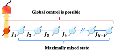
Figure 1: Hamiltonian identification model. A quantum probe is coupled to one end of the spin chain. A part from the quantum sensor (red spin), the rest of the spins (blue spins) are initially in the maximally mixed state. We further assume that we only have selective control on the quantum probe and global control on the spin chain.

V.1 Ising model without transverse field

As a preliminary example of the methods, we consider the Ising model without transverse field:

$$H=\sum_{k=1}^{N-1}\frac{J_{k}}{2}S_{k}^{\alpha}S_{k+1}^{\alpha}.$$ (8)

For concreteness, we can select $S^{\alpha}=X$ and $G_{0}=\{Z_{1}\}$ without loss of generality. The accessible set is easily obtained from the commutators and it saturates very quickly:

$$G=\{Z_{1},Y_{1}X_{2}\}.$$

Then, only the spin directly interacting with the quantum probe becomes correlated with it during the evolution and its parameter can be identified. As a consequence, $\text{rank}(\mathbf{A})=2$ and full Hamiltonian identification is only possible for $N=2$. Physically, this can be understood by a lack of information propagation in the Ising spin chain, which prevents the quantum probe at its end to gain information about the rest of the system. Indeed, the group velocity for information propagation in the Ising chain is zero.

Let the initial coherent vector be $\mathbf{x}(0)=(1,0)^{T}$ and the output matrix $\mathbf{C}=\begin{pmatrix}1&0\end{pmatrix}$. Then, the transfer function is:

$$T(s)=\frac{s}{s^{2}+J_{1}^{2}},$$

where we can identify $z_{1}=J_{1}^{2}$. Through ERA, we can obtain a new transfer function from the experimental data, which can be written in the most generality as

$$T_{\text{est}}(s)=\frac{s+b_{0}}{s^{2}+b_{1}^{2}s+a_{1}^{2}}.$$

Here we fixed the transfer function order to 2, as expected from the Ising model evolution. However, the form of $T_{\text{est}}(s)$ might differ from the ideal $T(s)$: in particular we might have additional terms, with coefficients $b_{j}$ arising from experimental errors or numerical approximations. Since $a_{1}^{2}$ reflects the contribution of $J_{1}^{2}$, we still expect $b_{j}^{2}\ll a_{1}^{2}$, and $b_{j}$’s are negligible. Therefore, the Gröbner basis is simply given by: $\mathscr{G}=\{z_{1}-a_{1}^{2}\}=\{J_{1}^{2}-a_{1}^{2}\}$ and the $N=2$ Ising chain can be identified with $\lambda_{\text{min}}=4$ sampling points.

We note that an alternative way of estimating $J_{1}$ is to measure the quantum probe (in particular $Z_{1}$) at known times. However, due to the periodicity of the signal, $J_{1}$ cannot be identified uniquely, even if measuring more than one time point.

We can thus generally state the following result.

Result 1.

The Ising model without the transversefield is only identifiable via the measurement of a sinlge probe spin for $N=2$, and the lower bound in the number of sampling points is given by: $\lambda_{\text{min}}=2\,\text{rank}(\mathbf{A})=4$.

V.2 Ising model with transverse field

Adding a transverse field to the Ising model drastically changes the system dynamics and consequently its identifiability.

The Hamiltonian is now

$$H=\sum_{k=1}^{N}\frac{\omega_{k}}{2}S^{\gamma}_{k}+\sum_{k=1}^{N-1}\frac{J_{k}}{2}S_{k}^{\alpha}S_{k+1}^{\alpha},$$

where for concreteness we will set $S^{\alpha}=X$ and $S^{\gamma}=Z$. There are several possible observable sets $G_{0}$ to choose from, as none of the operators $S^{\xi}_{1}$ ($\xi=\{\alpha,\beta,\gamma\}$) commute with the Hamiltonian. For the case considered, setting either $G_{0}=\{X_{1}\}$ or $\{Y_{1}\}$ is the best choice, as $G_{0}=\{Z_{1}\}$ would result in a larger-size $\tilde{\mathbf{A}}$. Either $G_{0}=\{X_{1}\}$ or $\{Y_{1}\}$ yields the accessible set:

$$\begin{split}G=\{X_{1},Y_{1},&Z_{1}X_{2},Z_{1}Y_{2},\cdots,\\ &Z_{1}\cdots Z_{N-1}X_{N},Z_{1}\cdots Z_{N-1}Y_{N}\},\end{split}$$

so that $\text{dim}(G)=2N$. All the chain spins are thus correlated with the quantum probe and we can hope to identify all the parameters. The system matrix $\tilde{\mathbf{A}}$ is a $2N\times 2N$ skew-symmetric matrix with the only non-zero elements $\tilde{\mathbf{A}}_{2k,2k-1}=\omega_{k}$ and $\tilde{\mathbf{A}}_{2k+1,2k}=J_{k}$. Since $\text{dim}(G)=\text{rank}(\mathbf{A})$, we have: $\text{rank}(\mathbf{A})=2N$. Choosing the initial state of the quantum probe to be the eigenstate of $X_{1}$, we have:

$$\mathbf{x}(0)=(1,0\cdots,0)^{T}\in\mathbb{R}^{2N}$$

If we measure $X_{1}$, the output matrix is $\mathbf{C}=\begin{pmatrix}1&0&\cdots&0\end{pmatrix}\in\mathbb{R}^{2N}$. From ERA and Eq. (6), we arrive at the following shape of the Gröbner basis:

$$\mathscr{G}=\{\omega_{1}^{2}-a_{1}^{2}\cdots,\omega_{N}^{2}-a_{N}^{2},J_{1}^{2}-b_{1}^{2},\cdots,J_{N-1}^{2}-b_{N-1}^{2}\}$$

because in this case $\mathcal{I}$ generated from Eq. (6) is a maximal ideal of the form $\langle z_{1}-a_{1}^{2},\cdots,z_{N}-a_{N}^{2},z_{N+1}-b_{1}^{2},\cdots,z_{2N-1}-b_{N-1}^{2}\rangle\ (a_{l},b_{k}\in\mathbb{R})$, where $z_{l}=\omega_{l}^{2}\ (l=1,\cdots,N)$ and $z_{N+k}=J_{k}^{2}\ (k=1,\cdots,N-1)$. Since there is only one positive real solution for the magnitudes of all the parameters, the Hamiltonian is fully identifiable.

If we measure $Y_{1}$ with the initial state of the quantum probe being the eigenstate of $X_{1}$, the Gröbner basis is instead:

$$\begin{split}\mathscr{G}=\{\omega_{1}-a_{1},\ &\omega_{2}^{2}-a_{2}^{2},\cdots,\omega_{N}^{2}-a_{N}^{2},\\ &J_{1}^{2}-b_{1}^{2},\cdots,J_{N-1}^{2}-b_{N-1}^{2}\},\end{split}$$

showing that we can find the sign of $\omega_{1}$, in addition to identifying the magnitude of all other parameters.

Physically, this result shows that identifiability is connected to information propagation along the whole chain. Indeed, since we assumed that we can extract information from the system only through the probe spin at one end of the chain, propagation of information through the whole chain is necessary to reveal the system’s properties. Adding a transverse field to the Ising model enables this information propagation.

We can thus generally state the following result.

Result 2.

The Hamiltonian of the nearest-neighbor Ising model with transverse field is identifiable via measurement of a single quantum probe. The minimum number of sampling points for $N$ spins is $\lambda_{\text{min}}=2\text{rank}(\mathbf{A})=4N$.

V.3 Exchange model without transverse field

The exchange (XY) model is another example where information propagation allows Hamiltonian identification via single-probe measurement.

The Hamiltonian can be written as:

$$H=\sum_{k=1}^{N-1}\frac{J_{k}}{2}(S^{\alpha}_{k}S^{\alpha}_{k+1}+S^{\beta}_{k}S^{\beta}_{k+1}),$$ (9)

where for concreteness we will set $S^{\alpha}=X$ and $S^{\beta}=Y$. For this case, $G_{0}=\{X_{1}\}$ or $\{Y_{1}\}$ is the best choice because the corresponding accessible set has the smallest size. Choosing, e.g., $G_{0}=\{X_{1}\}$, we obtain the following accessible set

$$\begin{split}G=\{X_{1},&Z_{1}Y_{2},Z_{1}Z_{2}X_{3},Z_{1}Z_{2}Z_{3}Y_{4},\cdots,\\ &Z_{1}\cdots Z_{2m-2}X_{2m-1},Z_{1}\cdots Z_{2m-1}Y_{2m}\},\end{split}$$

for an even-number of spins in the chain, $N=2m~{}(\forall m\in\mathbb{N})$, and

$$\begin{split}G=\{X_{1},&Z_{1}Y_{2},Z_{1}Z_{2}X_{3},Z_{1}Z_{2}Z_{3}Y_{4},\cdots,\\ &Z_{1}\cdots Z_{2m-3}Y_{2m-2},Z_{1}\cdots Z_{2m-2}X_{2m-1}\},\end{split}$$

for an odd number, $N=2m-1~{}(\forall m\in\mathbb{N})$.

The accessible set has the smallest possible dimension, $\text{dim}(G)=N$. (If we had chosen $G_{0}=\{Z_{1}\}$, the accessible set dimension would have been $\text{dim}(G)=N^{2}$. Therefore, in the following discussion, we consider $G_{0}=\{X_{1}\}$.) As all the spins are correlated with the quantum probe, we can expect the Hamiltonian to be fully identifiable. The system matrix $\tilde{\mathbf{A}}$ becomes an $N\times N$ skew-symmetric matrix with the only non-zero elements $(\tilde{\mathbf{A}})_{k,k+1}=(-1)^{k}J_{k}$, which has the same form as the system matrix of the Ising model with the transverse field. Since $\text{dim}(G)=\text{rank}(\mathbf{A})$, we have $\text{rank}(\mathbf{A})=N$. Choosing the initial state of the quantum probe to be the eigenstate of $X_{1}$, we have:

$$\mathbf{x}(0)=(1,0,\cdots,0)^{T}\in\mathbb{R}^{N}.$$

Since we can only measure the quantum probe, the output matrix is $\mathbf{C}=\begin{pmatrix}1&0&\cdots&0\end{pmatrix}\in\mathbb{R}^{N}$. From ERA and Eq. (6), we arrive at the following shape of the Gröbner basis:

$$\mathscr{G}=\{J_{1}^{2}-a_{1}^{2},\cdots,J_{N-1}^{2}-a_{N-1}^{2}\},$$

where $a_{k}\in\mathbb{R}$. Therefore, the Hamiltonian is fully identifiable since we have only one positive real solution for the magnitudes of all the parameters.

We can thus generally state the following result.

Result 3.

The Hamiltonian of the nearest-neighbor exchange model without transverse field is identifiable via measurement of a single quantum probe. The minimum number of sampling points for $N$ spins is $\lambda_{\text{min}}=2\text{rank}(\mathbf{A})=2N$.

V.4 Exchange model with transverse field

Adding a transverse field to the exchange Hamiltonian complicates the situation, as there might be more than one solution to the identification problem. However, this can be resolved by performing the measurements on two different observables.

The Hamiltonian is now given by:

$$H=\sum_{k=1}^{N}\frac{\omega_{k}}{2}S^{\gamma}_{k}+\sum_{k=1}^{N-1}\frac{J_{k}}{2}(S^{\alpha}_{k}S^{\alpha}_{k+1}+S^{\beta}_{k}S^{\beta}_{k+1}),$$

where for concreteness we choose $S^{\alpha}=X$, $S^{\beta}=Y$, and $S^{\gamma}=Z$. Again, the best choice is either $G_{0}=\{X_{1}\}$ or $G_{0}=\{Y_{1}\}$ that both yield the following accessible set:

$$\begin{split}G=\{X_{1},Y_{1},Z_{1}X_{2},&Z_{1}Y_{2},Z_{1}Z_{2}X_{3},Z_{1}Z_{2}Y_{3},\cdots,\\ &Z_{1}\cdots Z_{N-1}X_{N},Z_{1}\cdots Z_{N-1}Y_{N}\},\end{split}$$

with $\text{dim}(G)=2N$. The system matrix is a $2N\times 2N$ skew-symmetric matrix with the only non-zero elements $(\tilde{\mathbf{A}})_{2k-1,2k}=\omega_{k}$ and $(\tilde{\mathbf{A}})_{2k+2,2k-1}=(\tilde{\mathbf{A}})_{2k,2k+1}=J_{k}$. Choosing the initial state of the quantum probe to be an eigenstate of $X_{1}$, we have:

$$\mathbf{x}(0)=(1,0\cdots,0)^{T}\in\mathbb{R}^{2N}.$$

If we measure $X_{1}$, then we have $\mathbf{C}=\begin{pmatrix}1&0&\cdots&0\end{pmatrix}\in\mathbb{R}^{2N}$. From ERA and Eq. (6), we can construct a zero-dimensional ideal radical $\sqrt{\mathcal{I}}$. From the shape lemma, we obtain the following Gröbner basis:

$$\begin{split}\mathscr{G}(\sqrt{\mathcal{I}})=\{&z_{1}^{\alpha}+q_{1}(z_{1}),\\ &z_{2}+q_{2}(z_{1}),\\ &\vdots\\ &z_{2N-1}+q_{2N-1}(z_{1})\},\end{split}$$

where $z_{l}=\omega_{l}^{2}\ (l=1,\cdots,N)$ and $z_{N+k}=J_{k}^{2}\ (k=1,\cdots,N-1)$. Note that $\alpha>\text{deg}(q_{j})$ and $\alpha\geq 2$. Here, $q_{j}(z_{1})$ is the univariate polynomial in $z_{1}$. In general $z_{1}$ could have multiple values, so that we could have multiple sets of real solutions of the system of polynomial equations. Therefore, in general, this model is not identifiable. If we measure $Y_{1}$ with the initial state of the quantum probe being the eigenstate of $X_{1}$, we also have the same situations. Therefore, the exchange model with transverse field is generally not identifiable if we only measure one observable.

This issue can be resolved by measuring two different basis operators. Suppose that we measure $X_{1}$ and $Y_{1}$ with initial coherent vector $\mathbf{x}(0)=(1,0,\cdots,0)^{T}\in\mathbb{R}^{2N}$. In this case, we collect the measurement data for two observables, so that the sampling matrix $\mathbf{C}$ becomes: $\mathbf{C}=\begin{pmatrix}1&1&\cdots&0\end{pmatrix}\in\mathbb{R}^{2N}$. Then the transfer function can be written as the sum of the one for $X_{1}$ and the one for $Y_{1}$:

$$T(s)=T^{(X_{1})}(s)+T^{(Y_{1})}(s),$$

where $T^{(X_{1})}(s)$ and $T^{(Y_{1})}(s)$ have order $2N$. Therefore, the order of the transfer function $T(s)$ is still $2N$. In order to obtain the new realization, we perform the singular value decomposition of two Hankel matrices, corresponding to $X_{1}$ and $Y_{1}$, respectively. Thus, we can obtain the following new transfer function:

$$T_{\text{est}}(s)=T_{\text{est}}^{(X_{1})}(s)+T_{\text{est}}^{(Y_{1})}(s).$$

From the identity $T(s)=T_{\text{est}}(s)$, the polynomial ideal turns out to be a maximal ideal, which has the form of:

$$\begin{split}\mathcal{I}=\langle z_{1}-a_{1},&\cdots,z_{N}-a_{N},\\ &z_{N+1}-b_{1}^{2},\cdots,z_{2N-1}-b_{N-1}^{2}\rangle,\end{split}$$

where $z_{k}=\omega_{k}$ and $z_{N+k}=J_{k}^{2}$ and $a_{k},b_{k}\in\mathbb{R}$. Therefore, the Gröbner basis becomes:

$$\begin{split}\mathscr{G}(\mathcal{I})=\{\omega_{1}-a_{1},&\cdots,\omega_{N}-a_{N},\\ &J_{1}^{2}-b_{1}^{2},\cdots,J_{N-1}^{2}-b_{N-1}^{2}\}.\end{split}$$

The Hamiltonian is now fully identifiable since we have only one positive real solution for the magnitudes of all the parameters, and in addition we can find the sign of $\omega_{k}$.

Note that in this case, since we need two measurements, we need $2\times 2\text{rank}(\mathbf{A})=8N$ sampling points in total. This result can be understood as follows. The information provided by the time evolution of only one observable is not sometimes enough to extract the exact values of the parameters, but we can obtain a set of possible solutions. However, additional information provided by different observables can allow us to exclude some solutions. For the exchange model with transverse field, we can restrict the set of solutions to only one solution by adding the information provided by $Y_{1}$ to the information provided by $X_{1}$. Hence, we can generally state the following result.

Result 4.

The Hamiltonian of the nearest-neighbor exchange model with transverse field is generally non-identifiable via the measurement on a single quantum probe if we only measure one observable. If we observe two observables, the Hamiltonian can be fully identified and furthermore we can determine the sign of the Zeeman splitting. In this case, the minimum number of sampling points for $N$ spins is $\lambda_{\text{min}}=4\text{rank}(\mathbf{A})=8N$.

V.5 Time required for identification of spin chains

By analyzing ERA procedure, we obtained bounds on the minimum number of sampling points required for Hamiltonian identification. In turns, this also leads to requirements on the minimum evolution time as well as the total time required for Hamiltonian identification.

Indeed, if some a priori information about the system is known, we can choose the maximum time step required by the sampling theorem, $\Delta t=\pi/\Omega_{\text{max}}$, where $\Omega_{\text{max}}$ is the maximum eigenvalue of the Hamiltonian. With the minimum number of sampling points, the longest evolution time is at lest $t_{\text{tot}}=(\lambda_{min}-1)\Delta t$: This time should be compared to the system coherence time. In addition, the overall Hamiltonian identification requires a time

$$t_{\text{id}}=\Big{(}\frac{\lambda_{min}-1}{2}\Delta t+t_{\textrm{dead}}\Big{)}\lambda_{min},$$ (10)

where $t_{\textrm{dead}}$ is the dead time associated with system initialization and readout.

We can further check that these time requirements are consistent with our intuitive physical picture that connects Hamiltonian identification to the propagation of information through the whole spin chain. Consider for example the exchange Hamiltonian, Eq. (9), with all equal couplings. We can assume that the spins are equally spaced, with $a$ the lattice constant, and $L=(N-1)a$ the length of the chain. The eigenvalues of the Hamiltonian in the first excitation manifold are then

$$\Omega_{n}=2J\cos\Big{(}\frac{n\pi}{N+1}\Big{)}=2J\cos(k_{n}a),\quad k_{n}=n\pi\frac{N-1}{L(N+1)},$$

with $n=1,2,\dots,N$. Then, the maximum angular frequency is

$${\Omega_{\text{max}}}=2{J}\cos\Big{(}\frac{\pi}{N+1}\Big{)}.$$

Since we need at least $2N$ sampling points, the longest evolution time is $t_{\text{tot}}=(2N-1)\pi/\Omega_{\text{max}}$. For large $N\gg 1$, we can simplify this to

$$t_{\text{tot}}\simeq\pi\frac{N}{J}.$$

In order for the quantum probe to extract information on the whole spin chain, information needs to propagate to the other end and back. We can compute the group velocity for the propagation of the initial excitation on the first (probe) spin from the Hamiltonian eigenvalues $\Omega(k)$ Ramanathan et al. (2011),

$$v_{g}=\Big{|}\frac{d\Omega(k)}{dk}\Big{|}_{\text{max}}=2Ja=\frac{2JL}{N-1}.$$

Then, the time required for the information to come back to the probe spin is approximately given by

$$\tau\simeq\frac{2L}{v_{g}}=\frac{N-1}{J}$$

Thus, for large $N\gg 1$, we have $\tau\simeq\frac{N}{J}$, in agreement with the result obtained from the mathematical requirements for system identification.

VI Identifiability with external control

Until now we have analyzed identifiability under the assumption that we can initialize, measure, and control only the probe qubit. We found that some Hamiltonians cannot be identified, since they do not generate enough correlations among the target spins, or equivalently they do not transport information about the probe spin excitation through the whole chain. If we relax these assumptions and allow for a minimum level of control on the target spins, the picture changes. For example, if the target spins can be controlled via collective rotations, it is possible to turn a nonidentifiable Hamiltonian into an identifiable one.

Consider, for example, the Ising Hamiltonian, Eq. (8), which we showed in Sec. V.1 to be nonidentifiable. Using a simple control sequence (see Fig. 2), we can generate an effective Hamiltonian Haeberlen (1976) that can now be identified, since in the limit of small inter-pulse delays it has the same form as the exchange Hamiltonian, Eq. (9). Similarly, we could use a simple spin-echo procedure to refocus the transverse field and identify the coupling Hamiltonian in Sec. V.4, without the need to measure two observables.

More precisely, periodic pulse sequences such as in Fig. 2 make the system evolve as if under an effective time-independent Hamiltonian averaged over the cycle time. The effective Hamiltonian can be approximated by a first order Magnus expansion Magnus (1954) (average Hamiltonian Haeberlen (1976)). In this limit, to analyze the identifiability, it is sufficient to consider the average Hamiltonian. The exact effective Hamiltonian will be identifiable as long as we can identify its approximation; however, its expression might be too complex and analytical results only available in the limit of small enough time interval $\delta t\ll 1$ between the pulses where the approximation holds.

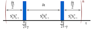
Figure 2: Identifiability with external control. By applying a periodic control pulse sequence $n$ times in the limit of a very small $J_{k}\delta t\ll 1$, we can transfer $H_{\text{is}}=\sum_{k=1}^{N-1}\frac{J_{k}}{2}S_{k}^{\alpha}S_{k+1}^{\alpha}$ to $H_{\text{ex}}=\sum_{k=1}^{N-1}\frac{J_{k}}{2}(S_{k}^{\alpha}S_{k+1}^{\alpha}+S_{k}^{\beta}S_{k+1}^{\beta})$ so that we can use $2N$ sampling points to identify the parameters $J_{k}$.

VII Robustness of ERA Hamiltonian identification

While previous works have already analyzed the robustness of the ERA procedure to experimental errors Hou et al. , here we want to evaluate the accuracy of the identification algorithm when it is implemented using only the minimum number of measurement points found above.

To compare with previous results, we consider the Ising model (with transverse field) for a chain of $N=3$ spins and the exchange model (without field) for a chain of $N=6$ spins. We consider the average error in 500 random Hamiltonian realizations and implement the ERA method, with the minimum number of measurement points ($\lambda_{\text{min}}=4N=12$ for the Ising model and $\lambda_{\text{min}}=2N=12$ points for the exchange Hamiltonian). We find that the relative error averaged over all the realization is still small ($10^{-10}-10^{-2}~{}[\%]$) and comparable to previous results, where many more points were measured.

Since the addition of experimental noise could change this result, we study the algorithm robustness in the presence of noise, as a function of the resources employed during the overall measurement process. To that end, we statistically compare the estimation robustness achieved by using Hankel matrices with different size but keeping fixed the experimental resources.

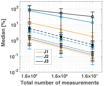
Figure 3: Estimation error with fixed time step $\Delta t$. Median of the estimation error $\{\langle\epsilon(J_{i})\rangle\}$ over $500$ random Hamiltonian realizations as a function of the total number of measurements. For each Hamiltonian, we repeated the ERA estimation $100$ times, to evaluate the average error $\langle\epsilon(J_{i})\rangle$. Solid lines with circles: $4\times 4$ Hankel matrix; dashed lines with solid square: $8\times 8$; dotted lines with squares: $40\times 40$. The error bars are the absolute median deviation.

We assume that each sampling point is measured $\mathcal{M}$ times, yielding a random outcome with a Gaussian distribution $\mathcal{N}(y(k),\sigma/\sqrt{\mathcal{M}})$, that is, we assume that the mean is centered around the “true outcome” value $y(k)$ at each time $k\Delta t$ and for simplicity consider a gaussian noise (with $\sigma=1$). By acquiring $2j$ sampling points (with $2j\mathcal{M}$ total measurements) we can construct the (noisy) $j\times j$ Hankel matrices $\tilde{\mathbf{H}}_{j}(0)$ and $\tilde{\mathbf{H}}_{j}(1)$. Using the ERA algorithm we can extract a set of parameters $\{\theta_{m}+\delta\theta_{m}\}_{m=1}^{M}$ that differ from the true parameters $\{\theta_{m}\}_{m=1}^{M}$. Since we are interested in the magnitude of the parameters, the estimation error can be written as:

$$\epsilon(\theta_{m})=\Big{|}\frac{|\theta_{m}+\delta\theta_{m}|-|\theta_{m}|}{|\theta_{m}|}\Big{|}\times 100~{}[\%].$$

In the simulations we repeat $r$ times this procedure in order to obtain the mean estimation error, $\langle\epsilon(\theta_{m})\rangle$ and we further take the median over many realizations of the input model parameters.

In our simulation, we compare the estimation errors for Hankel matrices of different sizes $j$, keeping however fixed the total number of measurements, $2j\mathcal{M}$. The smallest matrix has dimension $n\times n$, where $n$ is the model order. Larger matrices, of dimension $Ln\times Ln$, will thus have an increased error rate by a factor $\sqrt{L}$. Since the presence of the noise forces $\tilde{\mathbf{H}}_{Ln}(0)$ to be full-rank, we employ low-rank approximation via singular value decomposition Markovsky (2012) to generate an approximated $Ln\times Ln$ Hankel matrix with rank $n$.

We further consider two scenarios: either the time step $\Delta t$ is fixed (thus larger matrices require longer total times) or the total evolution time $T$ is fixed (reflecting, e.g., constraints imposed by decoherence or experimental drifts). In the first case, $\Delta t$ is chosen by assuming all the parameters take the possible maximal values so that the sampling theorem still holds. In the second case, we fix the total time evolution time to $T=(2n-1)\Delta t$ as required for the smallest Hankel matrix, and we use smaller time steps in the other cases

As an example, we focus on the $N=4$ exchange model without transverse field, which is shown in Eq. (9). The model order is given by $n=4$. Since we assume that the maximal possible value taken by coupling strengths is $100$, we have $dt=\frac{\pi}{25\sqrt{5}}$.

In Fig. 3 we plot the estimation errors $\{\langle\epsilon(J_{i})\rangle\}$ as a function of the total number of measurement for different Hankel matrix dimensions.

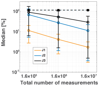
Figure 4: Estimation error with fixed total time $T$: Median of the estimation error $\{\langle\epsilon(J_{i})\rangle\}$ over $500$ random realizations of the Hamiltonian as a function of the total number of measurements. For each Hamiltonian, we repeated the ERA estimation $100$ times, to evaluate the averaged error. Solid lines with circles: $4\times 4$ Hankel matrix; dashed lines with solid square: $8\times 8$. The error bars are the absolute median deviation.

We note that the smallest Hankel matrix leads to larger errors, but already slightly larger matrices, possibly thanks to the low-rank approximation, give more accurate estimation. Indeed, thanks to the low-rank approximation, we generate a four-rank approximation of $\tilde{\mathbf{H}}_{4L}$ by neglecting the smallest singular values, which corresponds to an effective strategy for noise reduction. A second reason for the larger error is related to the shorter total time for the smallest Hankel matrix realization, that might in some cases not allow one to fully capture the smallest frequencies in the signal. While this is not typically an issue in the ideal case, in the presence of experimental noise this leads to higher estimation errors.

The role of the total time $T$ is highlighted when we consider the second scenario where $T$ is fixed: we fix the total time evolution time $T$ used for constructing $\tilde{\mathbf{H}}_{4}$, and compare the estimation performance between $\tilde{\mathbf{H}}_{4}$ and $\tilde{\mathbf{H}}_{8}$. Then, the time step for $\tilde{\mathbf{H}}_{8}$ is chosen to be $dt^{\prime}=\frac{7}{15}dt$. The result in Fig. 4 shows that in this case the larger Hankel matrix leads to larger errors although the time step $dt^{\prime}$ satisfies the sampling theorem. In the presence of noise, the additional sampling points acquired mostly contribute to increase the noise, but do not convey much more information. In addition, a very small time step might lead to larger errors, since it appears in the denominator of estimation equations [see, e.g., Eq. (31)].

VIII Discussion and conclusions

Hamiltonian identification is a central task in the quest of constructing ever more complex quantum devices as well as characterizing and imaging quantum systems in biology and materials science. To access these systems at their nano-scale, we proposed to use a quantum probe that coherently couples to their dynamics. In this scenario, we re-analyzed Hamiltonian identification via the eigensystem realization algorithm (ERA) approach and provided a systematic algorithm to test identifiability by employing the Gröbner basis. Even more importantly from a practical point of view, we showed that analyzing these techniques yields bounds on the experimental resources required to estimate the Hamiltonian parameters, both in terms of the minimum coherence time required for Hamiltonian identification and for the overall total experimental time for the multi-parameter estimate. These bounds can guide experimentalists in implementing the most efficient Hamiltonian identification protocol. We further numerically studied the estimation performance of ERA in the presence of noise. We found that the low-rank approximation for larger numbers of sampling points leads to more accurate estimation, even when the total number of measurements is kept fixed. This effects is however already at play for a small number of points above the minimum one, thus allowing one to keep the total evolution time short enough. When instead we fix the total evolution time as required to construct the smallest size Hankel matrix, there is no longer an advantage in using a larger number of sampling points, as the smaller time step leads to larger estimation errors. These analyses quantitatively provide helpful insights for a practical experimental approach to Hamiltonian identification based on ERA.

In order to obtain exemplary analytical results for our Hamiltonian identification protocol, we considered simple models of spin chains coupled by one end to the quantum probe. While these models are less complex than what would be found in practical experimental scenarios, they allowed us to clarify an interesting relation between Hamiltonian identifiability by a quantum probe and quantum information propagation in a chain. Indeed, as Hamiltonian identification relies on building a complete accessible set, the transport of information along the spin chain, in the form of spin-spin correlation, is a necessary condition. This result further imposes conditions on the time required for Hamiltonian identification: while in the cases we considered here these time bounds were consistent with the bounds directly imposed by ERA, it will be interesting to analyze in the future whether this result changes in the presence of disorder, when localization (either single particle or many-body) appears.

We finally showed that by relaxing some of the assumptions on control constraints, by allowing for example collective control of the target system, can turn a previously non-identifiable system into an identifiable one. These results can contribute to make Hamiltonian identification more experimentally practical in many real-system scenarios.

Appendix A Eigensystem Realization Algorithm

We review the eigensystem realization algorithm and how it can be applied Zhang and Sarovar (2014) for Hamiltonian identification assisted by single-probe measurement.

A.1 Construction of the state-space representation

For an interacting $N$ spin-1/2 system, the Hamiltonian can be written as

$$H=\sum_{m=1}^{M}\theta_{m}S_{m},$$ (11)

where $\theta_{m}\in\mathbb{R}\setminus\{0\}$ are the unknown parameters we want to determine, and $iS_{m}\in SU(2^{N})$. Let $\Gamma$ be the set of these Hermitian operators:

$$\Gamma=\{S_{m}|iS_{m}\in SU(2^{N})\},m=1,2,\cdots,M\},$$ (12)

with usually $M\ll 4^{N}-1$ due to the limitation in the number of spin couplings in the system. Let $G_{0}$ be the set of observables that we can measure. The choice of $G_{0}$ is discussed in Sec. II.1. We define the following iterative procedure:

$$G_{j}\equiv G_{j-1}\cup[G_{j-1},\Gamma],$$ (13)

where

$$[G_{j-1},\Gamma]\equiv\{O_{i}|\text{tr}(O_{i}^{\dagger}[\eta,\gamma])\neq 0,\eta\in G_{j-1},\gamma\in\Gamma\}.$$ (14)

Then, the finiteness in the dimension of $SU(2^{N})$ forces the iterative procedure to saturate, so that we can generate an accessible set $G$ of dimension $n\leq 4^{N}-1$:

$$G=\{O_{k}|iO_{k}\in SU(2^{N}),k=1,2,\cdots,n\}.$$ (15)

The physical meaning of $G$ was discussed in Sec. II.1.

The time evolution for each observable $O_{k}$ obeys Heisenberg’s equation:

$$\frac{dO_{k}}{dt}=i[H,O_{k}]=\sum_{l=1}^{n}\Big{(}\sum_{m=1}^{M}\theta_{m}V_{mkl}\Big{)}O_{l},$$ (16)

where

$$V_{mkl}=\text{Tr}(i[S_{m},O_{k}]O_{l})\in\mathbb{R}.$$ (17)

Let $\rho_{0}$ be the initial state of the system, and let us define $x_{k}=\text{Tr}(\rho_{0}O_{k})$. Eq. (16) can be written as

$$\frac{dx_{k}}{dt}=\sum_{l=1}^{n}\Big{(}\sum_{m=1}^{M}\theta_{m}V_{mkl}\Big{)}x_{l}$$ (18)

Defining a coherent vector $\mathbf{x}=(x_{1},\cdots,x_{n})^{T}\in\mathbb{R}^{n}$, we can rewrite Eq.  (18) into a compact form:

$$\frac{d\mathbf{x}(t)}{dt}=\tilde{\mathbf{A}}\mathbf{x}(t),$$ (19)

where the system matrix $\tilde{\mathbf{A}}\in\mathbb{R}^{n\times n}$ is a skew-symmetric matrix, i.e. $\tilde{\mathbf{A}}=-\tilde{\mathbf{A}}^{T}$. Let $y\in\mathbb{R}$ be the output data, which can be written in terms of the output matrix $\mathbf{C}\in\mathbb{R}^{n}$ as

$$y(t)=\mathbf{C}\mathbf{x}(t).$$ (20)

From Eq. (19) and Eq. (20), a state-space representation can be constructed as the following:

$$\begin{split}\frac{d\mathbf{x}(t)}{dt}&=\tilde{\mathbf{A}}\mathbf{x}(t)\\ y(t)&=\mathbf{C}\mathbf{x}(t).\end{split}$$ (21)

In discrete-time form, we have:

$$\begin{split}\mathbf{x}(j+1)&=\mathbf{A}\mathbf{x}(j)\\ y(j)&=\mathbf{C}\mathbf{x}(j),\end{split}$$ (22)

where $\mathbf{x}(j)\equiv\mathbf{x}(j\Delta t),y(j)\equiv y(j\Delta t)$ and

$$\mathbf{A}=e^{\tilde{\mathbf{A}}\Delta t}.$$ (23)

Since any matrix exponential is a nonsingular matrix, we have:

$$\text{rank}(\mathbf{A})=n.$$ (24)

From Eq. (21) we can obtain the transfer function $T(s)=\mathbf{C}(sI_{n}-\tilde{\mathbf{A}})^{-1}\mathbf{x}(0)$, and $[\tilde{\mathbf{A}},\mathbf{C},\mathbf{x}(0)]$ is called the realization of $T(s)$.

A.2 Realization Theory and Hankel matrix

The Hamiltonian identification algorithm Zhang and Sarovar (2014) relies on realization theory Katayama (2006). From the measurement data, we can construct the following Hankel matrix:

$$\mathbf{H}_{rs}(0)=\begin{pmatrix}y(0)&y(1)&\cdots&y(s-1)\\ y(1)&y(2)&\cdots&y(s)\\ \vdots&\vdots&\ddots&\vdots\\ y(r-1)&y(r)&\cdots&y(r+s-2)\end{pmatrix},$$ (25)

where we take $r,s\geq n$. In order to obtain the transfer function with the true model order $n$, we need $r,s\geq n$ because the rank of the Hankel matrix is equal to the order of the transfer function. Suppose that $r,s<n$, meaning that one takes fewer observations. In general, the rank of a $r\times s$ matrix cannot be greater than either $r$ or $s$; therefore, we have:

$$\text{rank}(\mathbf{H}_{rs}(0))\leq\text{min}(r,s)<n.$$

This means that a transfer function constructed from this smaller Hankel matrix would not have the true model order $n$. Therefore, $r$ and $s$ must satisfy $r,s\geq n$, and this is a necessary condition for ERA.

The Hankel matrix can be decomposed into

$$\mathbf{H}_{rs}(0)=\mathcal{O}_{r}\mathcal{C}_{s},$$ (26)

where $\mathcal{O}_{r}\in\mathbb{R}^{rn\times n}$ and $\mathcal{C}_{s}\in\mathbb{R}^{n\times sn}$ are called observability and controllability matrix, respectively, with:

$$\begin{split}\mathcal{O}_{r}&=\begin{pmatrix}\mathbf{C}\\ \mathbf{C}\mathbf{A}\\ \vdots\\ \mathbf{C}\mathbf{A}^{r-1}\end{pmatrix}\\ \mathcal{C}_{s}&=\begin{pmatrix}\mathbf{x}(0)&\mathbf{A}\mathbf{x}(0)&\cdots&\mathbf{A}^{s-1}\mathbf{x}(0)\end{pmatrix}.\end{split}$$ (27)

The singular value decomposition of $\mathbf{H}_{rs}(0)$ yields:

$$\mathbf{H}_{rs}(0)=\mathbf{U}\begin{pmatrix}\bf{\Sigma}&\mathbf{O}\\ \mathbf{O}&\mathbf{O}\end{pmatrix}\mathbf{V}^{T}=\begin{pmatrix}\mathbf{U}_{1}&\mathbf{U}_{2}\end{pmatrix}\begin{pmatrix}\bf{\Sigma}&\mathbf{O}\\ \mathbf{O}&\mathbf{O}\end{pmatrix}\begin{pmatrix}\mathbf{V}_{1}^{T}\\ \mathbf{V}_{2}^{T}\end{pmatrix}$$ (28)

where $\mathbf{U}$ and $\mathbf{V}$ are unitary matrices of dimensions $rn\times rn$ and $sn\times sn$, respectively. Let $l\leq n$ be the number of non-zero singular values of $\mathbf{H}_{rs}(0)$. $\bf{\Sigma}$ is the $l\times l$ diagonal matrix containing the non-zero singular values. Therefore, the observability and controllability matrices become:

$$\begin{split}\mathcal{O}_{r}&=\mathbf{U}_{1}\bf{\Sigma}^{1/2}\\ \mathcal{C}_{s}&=\bf{\Sigma}^{1/2}\mathbf{V}_{1}^{T}.\end{split}$$ (29)

By introducing the shifted-Hankel matrix:

$$\mathbf{H}_{rs}(1)=\begin{pmatrix}y(1)&y(2)&\cdots&y(s)\\ y(2)&y(3)&\cdots&y(s+1)\\ \vdots&\vdots&\ddots&\vdots\\ y(r)&y(r+1)&\cdots&y(r+s-1)\end{pmatrix}=\mathcal{O}_{r}\mathbf{A}\mathcal{C}_{s},$$ (30)

from Eq. (30) and Eq. (29), we can obtain the following new realization of the transfer function: $[\tilde{\mathbf{A}}_{\text{est}},\mathbf{C}_{\text{est}},\mathbf{x}_{\text{est}}(0)]$ such that:

$$\begin{split}\mathbf{x}_{\text{est}}(0)&=(\mathcal{O}_{r})_{\text{first column}}\\ \mathbf{C}_{\text{est}}&=(\mathcal{C}_{s})_{\text{first row}}\\ \tilde{\mathbf{A}}_{\text{est}}&=\frac{1}{\Delta t}\ln[\mathcal{O}_{r}^{-1}\mathbf{H}_{rs}(1)\mathcal{C}_{s}^{-1}].\end{split}$$ (31)

We write the corresponding transfer fuction as

$$T_{\text{est}}(s)=\mathbf{C}_{\text{est}}(sI_{n}-\tilde{\mathbf{A}}_{\text{est}})^{-1}\mathbf{x}_{\text{est}}(0),$$ (32)

and, in principle, $T(s)=T_{\text{est}}(s)$. In order to obtain the new realization, the system is required to be both observable and controllable. Therefore, the controllability and observability matrix must satisfy:

$$\begin{split}\text{rank}(\mathcal{C}_{s})&=n=\text{rank}(\mathbf{A})\\ \text{rank}(\mathcal{O}_{r})&=n=\text{rank}(\mathbf{A}).\end{split}$$ (33)

In turns, their ranks are determined by the Hankel matrix’s rank, as required by the Sylvester inequality: for $\mathbf{P}\in\mathbb{R}^{m\times k}$, $\mathbf{Q}\in\mathbb{R}^{k\times n}$,

$$p+q-k\leq\text{rank}(\mathbf{PQ})\leq\text{min}\{p,q\},$$

where $p=\text{rank}(\mathbf{P})$ and $q=\text{rank}(\mathbf{Q})$. From Eq. (30) and Eq. (33), the rank of the Hankel matrix must be:

$$\text{rank}(\mathbf{H}_{rs}(0))=n=\text{rank}(\mathbf{A}),$$ (34)

which indicates that the minimum dimension of the Hankel matrix and the shifted Hankel matrix is $n\times n$. Therefore, all the output data $\{y(0),\dots,y(2n-1)\}$ need to be recorded, which means that we require at least $2n$ sampling points in order to obtain the new realization of the system and thus extract the unknown parameters. From Eq. (24), the lower bound in the number of sampling points $\lambda_{\text{min}}$ is given by:

$$\lambda_{\text{min}}=2\text{rank}(\mathbf{A}).$$ (35)

Appendix B Basic theory of Gröbner basis

In this section, we review the basic theory of the Gröbner basis introduced in Cox et al. (2015, 2005); Fröberg (1997); Becker and Weispfenning (1998).

B.1 Monomial, polynomial, and monomial ordering

Let $\mathbb{Z}_{\geq 0}$ be the set of all nonnegative integers. A monomial in $z_{1},\cdots,z_{n}$ is the product $z_{1}^{\alpha_{1}}\cdots z_{n}^{\alpha_{n}}$, where $\alpha_{1},\cdots,\alpha_{n}\in\mathbb{Z}_{\geq 0}$. For simplicity, let us introduce the vectors $z=(z_{1},\cdots,z_{n})\in k^{n}$ and $\alpha=(\alpha_{1},\cdots,\alpha_{n})\in\mathbb{Z}_{\geq 0}^{n}$. Then, we write monomials as $z^{\alpha}\equiv z_{1}^{\alpha_{1}}\cdots z_{n}^{\alpha_{n}}$ and the monomial degree is

$$|\alpha|=\sum_{k=1}^{n}\alpha_{k}.$$ (36)

A polynomial $f\in k[z_{1},\cdots,z_{n}]$ is a finite linear combination of the monomials with coefficients in a field $k$:

$$f=\sum_{\alpha}c_{\alpha}z^{\alpha},\ \ c_{\alpha}\in k.$$ (37)

Monomial ordering is an important ingredient in all algorithms developed in commutative algebra. Let us introduce the so-called lexicographic order (lex) that we adapt to the Hamiltonian identification problem. Suppose we have $\alpha=(\alpha_{1},\cdots,\alpha_{n})\in\mathbb{Z}_{\geq 0}^{n}$ and $\beta=(\beta_{1},\cdots,\beta_{n})\in\mathbb{Z}_{\geq 0}^{n}$. If the leftmost nonzero entry of $\alpha-\beta\in\mathbb{Z}^{n}$ is positive, we write $\alpha\succ_{lex}\beta$ or $z^{\alpha}\succ_{lex}z^{\beta}$. For each variable $z_{1},\cdots,z_{n}$, the variables are ordered in the following way according to the lex ordering: $z_{1}\succ_{lex}z_{2}\succ_{lex}\cdots\succ_{lex}z_{n}$. By fixing the monomial ordering $\succ$, we can define the following terms.

1. The multidegree of a polynomial $f$ is : $\text{multideg}(f)=\text{max}(\alpha\in\mathbb{Z}_{\geq 0}^{n}|c_{\alpha\neq 0})$ with respect to $\succ$.

2. The leading coefficient of a polynomial $f$ is: $\text{LC}(f)=c_{\text{multideg}(f)}\in k$.

3. The leading monomial of $f$ is $\text{LM}(f)=x^{\text{multideg}(f)}.$

4. The leading term is $\text{LT}(f)=\text{LC}(f)\cdot\text{LM}(f)$.

B.2 Ideals and affine variety

Let $k$ be a commutative ring. A subset $I\subseteq k$ is called an ideal if it satisfies the following conditions:

1. $0\in I$.

2. If $f,g\in I$, then $f+g\in I$.

3. If $f\in I$ and $h\in k$, then $hf\in I$.

We are in particular interested in polynomial ideals. We denote the set of all polynomials in $z_{1},\cdots,z_{n}$ with coefficients on a field $k$ by $k[z_{1},\cdots,z_{n}]$. Then, a subset $\mathcal{I}=\langle f_{1},\cdots,f_{p}\rangle\subseteq k[z_{1},\dots,z_{n}]$ such that:

$$\mathcal{I}=\langle f_{1},\cdots,f_{p}\rangle=\Big{\{}\sum_{k=1}^{p}h_{k}f_{k}\Big{|}h_{1},\cdots,h_{p}\in k[z_{1},\cdots,z_{n}]\Big{\}}$$ (38)

is an ideal of $k[z_{1},\cdots,z_{n}]$. We call $\mathcal{I}$ a polynomial ideal generated by $f_{1},\cdots,f_{p}$, and $f_{1},\cdots,f_{p}$ are called the bases of the polynomial ideal $\mathcal{I}$.

The radical of $\mathcal{I}$ is defined by:

$$\sqrt{\mathcal{I}}=\{f\in k[z_{1},\cdots,z_{n}]|f^{k}\in\mathcal{I}\ \text{for some integer}\ k\geq 1\},$$ (39)

and we always have $\mathcal{I}\subseteq\sqrt{\mathcal{I}}$. Particularly, when $\mathcal{I}=\sqrt{\mathcal{I}}$, $\mathcal{I}$ is called a radical ideal.

Let $\mathbf{V}(f_{1},\cdots,f_{p})$ be the set of solutions of a system of polynomial equations, i.e.

$$\mathbf{V}(f_{1},...,f_{p})\!=\!\{(a_{1},...,a_{n})\!\in\!k^{n}\,|\,f_{l}(a_{1},...,a_{n})\!=\!0\},$$ (40)

for $l=1,2,\cdots,p$. $\mathbf{V}(f_{1},\cdots,f_{p})$ is called the affine variety defined by $f_{1},\cdots,f_{p}$. If $\{f_{1},\cdots,f_{p}\}$ and $\{g_{1},\cdots,g_{s}\}$ are the bases of the same polynomial ideal $\mathcal{I}$, then $\mathbf{V}(f_{1},\cdots,f_{p})=\mathbf{V}(g_{1},\cdots,g_{s})$. Any polynomial ideal $\mathcal{I}$ always satisfies:

$$\mathbf{V}(\sqrt{\mathcal{I}})=\mathbf{V}(\mathcal{I}),$$ (41)

and, particularly, if $k$ is an algebraically closed field $\mathbb{C}$, the affine variety and the radical ideal are in one-to-one correspondence.

B.3 Gröbner basis

For a polynomial ideal $\mathcal{I}\in k[z_{1},\cdots,z_{n}]\setminus\{0\}$, fixing a monomial order $\succ$, we define the leading term of the ideal, $\text{LT}(\mathcal{I})=\{\text{LT}(f)|\exists f\in\mathcal{I}\setminus\{0\}\}$, and we write the monomial ideal generated by the elements of $\text{LT}(\mathcal{I})$ as $\langle\text{LT}(\mathcal{I})\rangle$. If $\mathcal{I}=\langle f_{1},\cdots,f_{p}\rangle$, we always have $\text{LT}(f_{k})\in\text{LT}(\mathcal{I})\subseteq\langle\text{LT}(\mathcal{I})\rangle$.

From the Hilbert basis theorem Cox et al. (2005), every polynomial ideal $\mathcal{I}\setminus\{0\}$ has a finite generating set $\mathcal{G}(\mathcal{I})=\{g_{1},\cdots,g_{t}\}$, which satisfies $\langle\text{LT}(\mathcal{I})\rangle=\langle\text{LT}(g_{1}),\cdots,\text{LT}(g_{t})\rangle$. $\mathcal{G}(\mathcal{I})$ is called a Gröbner basis for the polynomial ideal $\mathcal{I}$. Therefore, the Hilbert basis theorem suggests that every polynomial ideal has a corresponding Gröbner basis. By adding the following restrictions:

1. every polynomial $g_{j}$ is monic. i.e. $\text{LC}(g_{j})=1$;

2. for every set of two distict polynomial $g_{j}$ and $g_{i}$, $\text{LM}(g_{j})$ is not divisible by $\text{LM}(g_{i})$ for any $i\neq j$,

we can obtain a unique minimal basis. The Gröbner basis with these restrictions is called reduced Gröbner basis, which is denoted by $\mathscr{G}(\mathcal{I})$.

B.4 Buchberger’s algorithm for constructing the Gröbner basis

The Gröbner basis can be constructed by Buchberger’s algorithm Buchberger (2006). Let $S_{i,j}$ be the S-polynomial of the pair $(f_{i},f_{j})$, which is defined as:

$$S_{i,j}=\frac{\text{LCM}[\text{LM}(f_{i}),\text{LM}(f_{j})]}{\text{LM}(f_{i})}f_{i}-\frac{\text{LCM}[\text{LM}(f_{i}),\text{LM}(f_{j})]}{\text{LM}(f_{j})}f_{j},$$ (42)

where $\text{LCM}[\text{LM}(f_{i}),\text{LM}(f_{j})]$ denotes the least common multiple of $\text{LM}(f_{i})$ and $\text{LM}(f_{j})$. Let $\text{rem}(S_{i,j},G)$ be the remainder of dividing $S_{i,j}$ by all elements in $G$. Let us consider the ideal $\mathcal{I}\subset\mathbb{C}[z_{1},\cdots,z_{n}]$ generated by $f_{1},\cdots,f_{p}$. Buchberger’s algorithm Cox et al. (2015) is given by:

  INPUT: $F=\{f_{1},\cdots,f_{p}\}$

  OUTPUT: The Gröbner basis $\mathscr{G}(\mathcal{I})=\{g_{1},\cdots,g_{t}\}$ for the ideal $\mathcal{I}$.

  $G:=F$

  repeat

     $G^{\prime}:=G$

     for all $\{f_{i},f_{j}\},i\neq j$ in $G^{\prime}$ do

        $R:=\text{rem}(S_{i,j},G^{\prime})$

        if $R\neq 0$ then

           $G:=G\cup\{\text{rem}(S_{i,j},G^{\prime})\}$

        end if

     end for

  until $G=G^{\prime}$

  RETURN $G$

B.5 Construction of radicals of zero-dimensional ideal

Let us consider the following system of polynomial equations:

$$\begin{split}f_{1}&(z_{1},\cdots,z_{n})=0\\ f_{2}&(z_{1},\cdots,z_{n})=0\\ &\vdots\\ f_{p}&(z_{1},\cdots,z_{n})=0\end{split}$$ (43)

and $f_{1},\cdots,f_{p}\in\mathbb{C}[z_{1},\cdots,z_{n}]$. Suppose that Eq. (43) has a finite set of solutions. Then, the polynomial ideal $\mathcal{I}$ generated by $f_{1},\cdots,f_{n}$ is called zero-dimensional ideal. Here, let us introduce the procedure to construct the radical $\sqrt{\mathcal{I}}$. By Buchberger’s algorithm and the definition of the reduced Gröbner basis, we can obtain the following reduced Gröbner basis:

$$\begin{split}\mathscr{G}(\mathcal{I})=\{&g_{1}(z_{1}),\\ &g_{2,1}(z_{1},z_{2}),\cdots,g_{2,v_{2}}(z_{1},z_{2}),\\ &\vdots\\ &g_{M,1}(z_{1},\cdots,z_{M}),\cdots,g_{M,v_{M}}(z_{1},\cdots,z_{M})\}.\end{split}$$ (44)

and $\mathscr{G}(\mathcal{I})$ generates the same ideal. Let $h_{j}$ be an unique monic generator of the elimination ideal $\mathcal{I}\cap\mathbb{C}[z_{j}]$. Then, we can choose $h_{j}$ such that $h_{j}\in\mathscr{G}(\mathcal{I})\cap\mathbb{C}[z_{j}]$ by the elimination theorem. Let $\varphi_{j}(z_{j})$ be $\varphi_{j}=h_{j}/\text{gcd}(h_{j},\partial_{z_{j}}h_{j})$, the radical of the zero-dimensional ideal $\mathcal{I}$ is given by:

$$\sqrt{\mathcal{I}}=\mathcal{I}+\langle\varphi_{1},\cdots,\varphi_{n}\rangle.$$ (45)

(See e.g.,  Becker and Weispfenning (1998) for the proof). In particular, by Seidenberg’s Lemma Becker and Weispfenning (1998), when $\varphi_{j}=1$, $\mathcal{I}$ is a radical zero-dimensional ideal, and the Gröbner basis for the radical zero-dimensional ideal has a special shape, as described by the shape lemma Cox et al. (2005), such that:

$$\mathscr{G}=\{z_{1}^{\alpha}+q_{1}(z_{1}),\cdots,z_{n-1}+q_{n-1}(z_{1}),z_{n}+q_{n}(z_{1})\},$$ (46)

where $\alpha\in\mathbb{N}$ and $q_{j}(z_{1})$ are the univariate polynomials in $z_{1}$ with degree $\text{deg}(q_{j})<\alpha$.

B.6 Elimination theory

Let $\mathcal{I}\subseteq k[z_{1},\cdots,z_{n}]$ be a polynomial ideal. Let us define $\mathcal{I}_{l}$ by:

$$\mathcal{I}_{l}=\mathcal{I}\cap k[z_{l+1},\dots,z_{n}],$$ (47)

and we call $\mathcal{I}_{l}$ the $l$-th elimination ideal. Fixing the lex order $z_{1}\succ_{lex}z_{2}\succ_{lex}\cdots\succ_{lex}z_{n}$, for every $l$, the Gröbner basis for the $l$-th elimination ideal is written by:

$$\mathcal{G}_{l}=\mathcal{G}\cap k[z_{l+1},\cdots,z_{n}],$$ (48)

where $\mathcal{G}$ is the Gröbner basis for $\mathcal{I}$ (elimination theorem) Cox et al. (2015).

By employing the elimination theorem, we can derive the shape of the reduced Gröbner basis in Sec. V.2 and Sec. V.3. Let us take $\mathbf{x}(0)=(1,0,\cdots,0)^{T}\in\mathbb{R}^{n+1}$, and $\mathbf{C}=\begin{pmatrix}1&0&\cdots&0\end{pmatrix}\in\mathbb{R}^{n+1}$. The system matrix $\tilde{\mathbf{A}}$ is an $(n+1)\times(n+1)$ skew-symmetric matrix with the only non-zero elements $\theta_{k}=(\tilde{\mathbf{A}})_{k+1,k}=-(\tilde{\mathbf{A}})_{k,k+1}$, where $k=1,2,\cdots,n$. Then, from Eq. (6), we obtain the following system of polynomial equations:

$$f_{1}(z_{1},\cdots,z_{n})=\cdots=f_{n}(z_{1},\cdots,z_{n})=0,$$ (49)

where $z_{k}=\theta_{l}^{2}\ (k,l=1,2,\cdots,n)$. We can construct a polynomial ideal

$$\mathcal{I}=\langle f_{1},\cdots,f_{n}\rangle\in\mathbb{C}[z_{1},\cdots,z_{n}].$$ (50)

Note that for convenience we consider the polynomial ideal over the polynomial ring $\mathbb{C}[z_{1},\cdots,z_{n}]$. In this case, we have found that there exists a proper choice for the pair $(k,l)$ such that the corresponding elimination ideal $\mathcal{I}_{l-1}$ has the basis $z_{k}-c_{k}^{2}$ for $\exists c_{k}\in\mathbb{R}$, meaning that:

$$z_{k}-c_{k}^{2}\in\mathcal{G}_{l-1}.$$ (51)

From the elimination theorem, we have:

$$\begin{split}\mathcal{G}_{l-1}&=\mathcal{G}\cap\mathbb{C}[z_{l},\cdots,z_{n}]\\ &=\mathcal{G}\cap(\mathbb{C}[z_{l}]\cup\mathbb{C}[z_{l+1},\cdots,z_{n}])\\ &=(\mathcal{G}\cap\mathbb{C}[z_{l}])\cup(\mathscr{G}\cap\mathbb{C}[z_{l+1},\cdots,z_{n}])\\ &=(\mathcal{G}\cap\mathbb{C}[z_{l}])\cup\mathcal{G}_{l},\end{split}$$ (52)

which yields:

$$\mathcal{G}_{l}\subset\mathcal{G}_{l-1}.$$ (53)

Therefore, we can inductively obtain:

$$\mathcal{G}_{n-1}\subset\mathcal{G}_{n-2}\subset\cdots\subset\mathcal{G}_{2}\subset\mathcal{G}_{1}\subset\mathcal{G}.$$ (54)

By the definition of the reduced Gröbner basis, $\mathscr{G}(\mathcal{I})$ has the shape:

$$\mathscr{G}(\mathcal{I})=\langle z_{1}-a_{1},\cdots,z_{n}-a_{n}\rangle,$$ (55)

where $a_{k}=c_{l}^{2}$. This tells us the fact that $\mathcal{I}$ is the maximal ideal of $\mathbb{C}[z_{1},\cdots,z_{n}]$.

B.7 Comments on efficiency of Gröbner basis

The computation of Gröbner basis takes tremendously large complexity Cox et al. (2015). Let $F$ be a set of polynomials $\{f_{1},\cdots,f_{t}\}$ in $z_{1},\cdots,z_{n}\in\mathbb{C}$, and let $d$ be the maximal multiple degree of the input polynomials, i.e. $d=\text{max}(\text{multideg}(f_{1}),\cdots,\text{multideg}(f_{t}))$. Suppose that $F$ generates a zero-dimensional ideal. Then, the complexity for computing the reduced Gröbner basis can be given by $d^{O(n)}$ Lakshman and Lazard (1991). Therefore, for a larger system, the Gröbner basis takes a tremendously long time due to its complexity. Efficiency improvement of computing Gröbner basis is a timely problem. For example, recently, Gritzmann and Sturmfels proposed the idea of dynamic alternation of the monomial ordering while the algorithm progresses Gritzmann and Sturmfels (1993); Caboara and Perry (2014). Therefore, we expect that the current research efforts on the development efficient computation method of Gröbner basis can definitely contribute to the reduction of the computation complexity in the Hamiltonian identification. We want to emphasize that the Gröbner basis approach is a fundamental and systematic way to solve the system of polynomial equations. More importantly, it is useful due to peculiar properties of its shape which can determine the solvability of the system of polynomial equations and hence the identifiability of the Hamiltonian. Therefore, learning the Hamiltonian identifiability by applying Gröbner basis is fundamentally essential and necessary.

Appendix C Examples of polynomials for identifiable Hamiltonians

In this section, we show the explicit polynomials for particular identifiable models.

C.1 $N=3$ Ising model with transverse field

For the Ising model with transverse field with $N=3$ spins, the Hamiltonian can be written as:

$$H=\sum_{k=1}^{3}\frac{\omega_{k}}{2}Z_{k}+\sum_{k=1}^{2}\frac{J_{k}}{2}X_{k}X_{k+1}.$$

Let us choose $G_{0}=\{X_{1}\}$ and let the initial state of the probe be the eigenstate of $X_{1}$ and the rest of spins in the chain be the maximally mixed state. The system matrix $\tilde{\mathbf{A}}$ is

$$\tilde{\mathbf{A}}=\begin{pmatrix}0&-\omega_{1}&0&0&0&0\\ \omega_{1}&0&-J_{1}&0&0&0\\ 0&J_{1}&0&-\omega_{2}&0&0\\ 0&0&\omega_{2}&0&-J_{2}&0\\ 0&0&0&J_{2}&0&-\omega_{3}\\ 0&0&0&0&\omega_{3}&0\end{pmatrix},$$

and output matrix $\mathbf{C}$ is given as

$$\mathbf{C}=\begin{pmatrix}1&0&0&0&0&0\end{pmatrix},$$

and the initial coherent vector is:

$$\mathbf{x}(0) =(1,0,0,0,0,0)^{T}.$$

Let us define $(z_{1},z_{2},z_{3},z_{4},z_{5})=(\omega_{1}^{2},\omega_{2}^{2},\omega_{3}^{2},J_{1}^{2},J_{2}^{2})$. Then, from Eq. (6), we can obtain the following form of the system of polynomial equations:

$$\begin{split}&z_{1}z_{2}z_{3}=v_{1}\\ &z_{1}z_{2}+z_{1}z_{3}+z_{2}z_{3}+z_{3}z_{4}+z_{1}z_{5}+z_{4}z_{5}=v_{2}\\ &z_{1}+z_{2}+z_{3}+z_{4}+z_{5}=v_{3}\\ &z_{2}z_{3}+z_{3}z_{4}+z_{4}z_{5}=v_{4}\\ &z_{2}+z_{3}+z_{4}+z_{5}=v_{5},\end{split}$$

where $v_{k}>0~{}(k=1,\cdots,5)$. Then, the Gröbner basis takes the following form: $\mathscr{G}=\{z_{1}-a_{1}^{2},z_{2}-a_{2}^{2},z_{3}-a_{3}^{2},z_{4}-a_{4}^{2},z_{5}-a_{5}^{2}\}$, where $\{a_{1}^{2},a_{2}^{2},a_{3}^{2},a_{4}^{2},a_{5}^{2}\}$ are given in Eq. (56):

$$\begin{split}a_{1}^{2}&=v_{3}-v_{5}\\ a_{2}^{2}&=\frac{v_{2}-v_{4}}{v_{3}-v_{5}}+\frac{v_{1}+v_{4}(v_{5}-v_{3})}{v_{4}-v_{2}+v_{5}(v_{3}-v_{5})}\\ a_{3}^{2}&=\frac{v_{1}(v_{4}-v_{2}+v_{5}(v_{5}-v_{3}))}{(v_{2}-v_{4})^{2}+v_{3}^{2}v_{4}-v_{3}v_{5}(v_{2}+v_{4})+v_{2}v_{5}^{2}+v_{1}(v_{5}-v_{3})}\\ a_{4}^{2}&=\frac{v_{4}-v_{2}}{v_{3}-v_{5}}\\ a_{5}^{2}&=-\frac{v_{1}}{v_{2}}+\frac{v_{1}-v_{4}(v_{3}-v_{5})}{v_{2}-v_{4}-v_{5}(v_{3}-v_{5})}+\frac{v_{1}(v_{1}(v_{5}-v_{3})+v_{4}(-v_{2}+v_{4}+v_{3}(v_{3}-v_{5})))}{v_{2}((v_{2}-v_{4})^{2}-v_{1}v_{3}+v_{3}^{2}v_{4}+v_{5}(v_{1}-v_{3}(v_{2}+v_{4}))+v_{2}v_{5}^{2})},\end{split}$$ (56)

C.2 $N=4$ Exchange model without transverse field

Next, let us consider the exchange model without transverse field with $N=4$ spins. The Hamiltonian can be written as:

$$H=\sum_{k=1}^{3}\frac{J_{1}}{2}(X_{k}X_{k+1}+Y_{k}Y_{k+1}).$$

Let us take same observable set and initial state of spin chain in Sec. C.1. The system matrix $\tilde{\mathbf{A}}$ is

$$\tilde{\mathbf{A}}=\begin{pmatrix}0&-J_{1}&0&0\\ J_{1}&0&J_{2}&0\\ 0&-J_{2}&0&-J_{3}\\ 0&0&J_{3}&0\end{pmatrix},$$

and output matrix $\mathbf{C}$ is given as

$$\mathbf{C}=\begin{pmatrix}1&0&0&0\end{pmatrix},$$

and the initial coherent vector is:

$$\mathbf{x}(0) =(1,0,0,0)^{T}.$$

Let us define $(z_{1},z_{2},z_{3})=(J_{1}^{2},J_{2}^{2},J_{3}^{2})$. Then, from Eq. (6), we can obtain the following form of the system of polynomial equations:

$$\begin{split}&z_{2}+z_{3}=v_{1}\\ &z_{1}z_{3}=v_{2}\\ &z_{1}+z_{2}+z_{3}=v_{3}\\ \end{split}$$

where $v_{k}>0~{}(k=1,\cdots,5)$. Then, the Gröbner basis takes the following form: $\mathscr{G}=\{z_{1}-a_{1}^{2},z_{2}-a_{2}^{2},z_{3}-a_{3}^{2}\}$, where $\{a_{1}^{2},a_{2}^{2},a_{3}^{2}\}$ are given in Eq. (57):

$$\begin{split}a_{1}^{2}&=v_{3}-v_{1}\\ a_{2}^{2}&=\frac{v_{1}v_{3}-v_{2}-v_{1}^{2}}{v_{3}-v1}\\ a_{3}^{3}&=\frac{v_{2}}{v_{3}-v1}\end{split}$$ (57)

where $v_{3}>v_{1}$, $v_{1}(v_{3}-v_{1})>v_{2}>0$.

C.3 $N=2$ Exchange model with transverse field

Finally, let us consider the exchange model with $N=2$ spins with transverse field. The Hamiltonian can be written as:

$$H=\frac{\omega_{1}}{2}Z_{1}+\frac{\omega_{2}}{2}Z_{2}+\frac{J_{1}}{2}(X_{1}X_{2}+Y_{1}Y_{2}).$$

In Sec. V.4, we have discussed that the Hamiltonian becomes fully identifiable if we measure $X_{1}$ and $Y_{1}$ separately. Let us always prepare the initial state of the spin probe to be the eigenstate of $\{X_{1}\}$ and the other spin to be the maximally mixed state. The system matrix is

$$\tilde{\mathbf{A}}=\begin{pmatrix}0&\omega_{1}&0&-J_{1}\\ -\omega_{1}&0&-J_{1}&0\\ 0&J_{1}&0&\omega_{2}\\ J_{1}&0&-\omega_{2}&0\end{pmatrix}.$$

Here, the output matrix becomes

$$\mathbf{C}=\begin{pmatrix}1&1&0&0\end{pmatrix}$$

and the initial coherent vector is

$$\mathbf{x}(0)=(1,0,0,0)^{T}.$$

Let us define $(z_{1},z_{2},z_{3})=(\omega_{1},\omega_{2},J_{1}^{2})$. Then, from Eq. (6), we can obtain the following form of the system of polynomial equations:

$$\begin{split}&-z_{1}z_{2}^{2}-z_{2}z_{3}=v_{1}\\ &z_{2}^{2}+z_{3}=v_{2}\\ &z_{1}=v_{3}\\ &(z_{1}z_{2}+z_{3})^{2}=v_{4}\\ &z_{1}^{2}+z_{2}^{2}+2z_{3}=v_{5}.\end{split}$$

Then, the Gröbner takes the following form: $\mathscr{G}=\{z_{1}-a_{1},z_{2}-a_{2},z_{3}-a_{3}^{2}\}$, where $\{a_{1},a_{2},a_{3}^{2}\}$ are given in Eq. (58):

$$\begin{split}a_{1}&=v_{3}\\ a_{2}&=\frac{v_{1}+2v_{2}v_{3}+v_{3}^{3}-v_{3}v_{5}}{v_{2}+v_{3}^{2}-v_{5}}\\ &=\frac{v_{2}^{2}-v_{2}v_{3}^{2}-v_{3}^{4}+v_{4}-v_{2}v_{5}+v_{3}^{2}v_{5}}{v_{1}-v_{3}^{3}+v_{3}v_{5}}\\ &=\frac{2v_{1}(v_{2}-v_{5})+v_{3}(-v_{2}^{2}+2v_{2}v_{3}^{2}+2v_{3}^{4}-3v_{4}-3v_{3}^{2}v_{5}+v_{5}^{2})}{2(v_{3}^{4}+v_{4}-v_{3}^{2}v_{5})}\\ a_{3}^{2}&=v_{5}-v_{2}-v_{3}^{2},\end{split}$$ (58)

where $v_{2}+v_{3}^{2}-v_{5}\neq 0$, $v_{1}-v_{3}^{2}+v_{3}v_{5}\neq 0$, $v_{3}^{4}+v_{4}-v_{3}^{2}v_{5}\neq 0$ and $v_{5}-v_{2}-v_{3}^{2}>0$. Here $a_{1}$ and $a_{2}$ are the nonzero real numbers. Also note that $\{v_{1},v_{2},v_{3},v_{4},v_{5}\}$ satisfy the following simultaneous identity:

$$v_{2}^{4}-4v_{2}^{3}v_{5}-2v_{2}^{2}(v_{4}+(v_{3}^{2}-3v_{5})v_{5})+(v_{4}-v_{5}^{2})^{2}+v_{3}^{4}(-4v_{4}+v_{5}^{2})+v_{3}^{2}(6v_{4}v_{5}-2v_{5}^{3})+4v_{2}(v_{5}(v_{4}-v_{5}^{2})+v_{3}^{2}(-2v_{4}+v_{5}^{2}))=0$$

$$-v_{2}^{2}+2v_{1}v_{3}+v_{4}+2v_{2}v_{5}+(v_{3}^{2}-v_{5})v_{5}=0$$

$$2v_{1}(-v_{4}+(v_{2}-v_{5})^{2})-v_{3}(4(2v_{2}+v_{3}^{2})v_{4}+(v_{2}^{2}-5v_{4})v_{5}-(2v_{2}+v_{3}^{2})v_{5}^{2}+v_{5}^{3})=0$$

$$v_{1}^{2}-v_{4}(2v_{2}+v_{3}^{2}-v_{5})=0.$$

References

- (1) A. Ajoy, Y. X. Liu, K. Saha, L. Marseglia, J.-C. Jaskula, U. Bissbort, and P. Cappellaro, arXiv:1604.01677 .
- Ajoy et al. (2015) A. Ajoy, U. Bissbort, M. D. Lukin, R. L. Walsworth, and P. Cappellaro1, Phys. Rev. X 5, 011001 (2015).
- Lovchinsky et al. (2016) I. Lovchinsky, A. O. Sushkov, E. Urbach, N. P. de Leon, S. Choi, K. De Greve, R. Evans, R. Gertner, E. Bersin, C. Müller, L. McGuinness, F. Jelezko, R. L. Walsworth, H. Park, and M. D. Lukin, Science 351, 836 (2016).
- Cooper et al. (2014) A. Cooper, E. Magesan, H. Yum, and P. Cappellaro, Nat. Commun. 5, 3141 (2014).
- Barry et al. (2016) J. F. Barry, M. J. Turner, J. M. Schloss, D. R. Glenn, Y. Song, M. D. Lukin, H. Park, and R. L. Walsworth, Proc. Natl. Acad. Sci. USA 113, 14133 (2016).
- van der Sar et al. (2014) T. van der Sar, F. Casola, R. Walsworth, and A. Yacoby, Nat. Commun. 6, 7886 (2014).
- Wolfe et al. (2016) C. S. Wolfe, S. A. Manuilov, C. M. Purser, R. Teeling-Smith, C. Dubs, P. C. Hammel, and V. P. Bhallamudi, App. Phys. Lett 108, 232409 (2016).
- Burgarth et al. (2009) D. Burgarth, K. Maruyama, and F. Nori, Phys. Rev. A 79, 020305(R) (2009).
- Burgarth and Maruyama (2009) D. Burgarth and K. Maruyama, New J. Phys. 11, 103019 (2009).
- Franco et al. (2009) C. D. Franco, M. Paternostro, and M. S. Kim, Phys. Rev. Lett. 102, 187203 (2009).
- (11) Y. Wang, D. Dong, B. Qi, J. Zhang, I. R. Petersen, and H. Yonezawa, arXiv:1610.08841 .
- Granade et al. (2012) C. E. Granade, C. Ferrie, N. Wiebe, and D. G. Cory, New J. Phys. 14, 103013 (2012).
- Schirmer and Langbein (2015) S. G. Schirmer and F. C. Langbein, Phys. Rev. A 91, 022125 (2015).
- Sergeevich et al. (2011) A. Sergeevich, A. Chandran, J. Combes, S. D. Bartlett, and H. M. Wiseman, Phys. Rev. A 84, 052315 (2011).
- Shabani et al. (2011) A. Shabani, M. Mohseni, S. Lloyd, R. L. Kosut, and H. Rabitz, Phys. Rev. A 84, 012107 (2011).
- Magesan et al. (2013) E. Magesan, A. Cooper, and P. Cappellaro, Phys. Rev. A 88, 062109 (2013).
- Arai et al. (2015) K. Arai, C. Belthangady, H. Zhang, N. Bar-Gill, S. DeVience, P. Cappellaro, A. Yacoby, and R. Walsworth, Nat. Nanotech. 10, 859 (2015).
- Zhang and Sarovar (2014) J. Zhang and M. Sarovar, Phys. Rev. Lett. 113, 080401 (2014).
- Zhang and Sarovar (2015) J. Zhang and M. Sarovar, Phys. Rev. A 91, 052121 (2015).
- (20) S.-Y. Hou, H. Li, and G.-L. Long, arXiv:1410.3940v1 .
- Maletinsky et al. (2012) P. Maletinsky, S. Hong, M. S. Grinolds, B. Hausmann, M. D. Lukin, R. L. Walsworth, M. Loncar, and A. Yacoby, Nat. Nanotech. 7, 320 (2012).
- Boss et al. (2016) J. M. Boss, K. Chang, J. Armijo, K. Cujia, T. Rosskopf, J. R. Maze, and C. L. Degen, Phys. Rev. Lett. 116, 197601 (2016).
- Ljung (1999) L. Ljung, System Identification: Theory for the User, 2nd edition (Prentice-Hall, Upper Saddle River, NJ, 1999).
- Katayama (2006) T. Katayama, Subspace methods for system identification (Springer Science and Business Media, London, 2006).
- Caicedo et al. (2014) J. M. Caicedo, S. J. Dyke, and E. A. Johnson, J. Eng. Mech. 130(1), 49 (2014).
- Moncayo et al. (2010) H. Moncayo, J. Marulanda, and P. Thomson, J. Aerospace. Eng. 23, 99 (2010).
- Cox et al. (2015) D. A. Cox, J. Little, and D. O’Shea, Ideals, Varieties, and Algorithms (An Introduction to Computational Algebraic Geometry and Commutative Algebra), 4th edition (Springer, Cham, 2015).
- Cox et al. (2005) D. A. Cox, J. Little, and D. O’Shea, Using Algebraic Geometry, 2nd edition (Springer, New York, 2005).
- Fröberg (1997) R. Fröberg, An Introduction to Gröbner basis (John Wiley & Sons, New York, 1997).
- Becker and Weispfenning (1998) T. Becker and V. Weispfenning, Gröbner basis: A Computational Approach to Commutative Algebra (Springer, New York, 1998).
- Buchberger (2006) B. Buchberger, J. Symb. Comput. 41, 475 (2006).
- Burgarth and Yuasa (2012) D. Burgarth and K. Yuasa, Phys. Rev. Lett. 108, 080502 (2012).
- Burgarth and Yuasa (2014) D. Burgarth and K. Yuasa, Phys. Rev. A 89, 030302(R) (2014).
- Guţǎ and Yamamoto (2016) M. Guţǎ and N. Yamamoto, IEEE Trans. Autom. Control. 921, 61 (2016).
- James et al. (2008) M. R. James, H. I. Nurdin, and I. R. Petersen, IEEE Trans Autom. Control. 53(8), 1787 (2008).
- Yamamoto (2014) N. Yamamoto, Phys. Rev. X 4, 041029 (2014).
- Li et al. (2009) G.-X. Li, S.-S. Ke, and Z. Ficek, Phys. Rev. A 79, 033827 (2009).
- Horn and Johnson (2013) R. A. Horn and C. R. Johnson, Matrix Analysis, 2nd edition (Cambridge University Press, New York, 2013).
- Shannon (1949) C. E. Shannon, Proc. IRE 37.1 (1949): 10-21. 37(1), 10 (1949).
- Bose (2003) S. Bose, Phys. Rev. Lett. 91, 207901 (2003).
- Franco et al. (2008) C. D. Franco, M. Paternostro, and M. S. Kim, Phys. Rev. Lett. 101, 230502 (2008).
- Cappellaro et al. (2011) P. Cappellaro, L. Viola, and C. Ramanathan, Phys. Rev. A 83, 032304 (2011).
- Ramanathan et al. (2011) C. Ramanathan, P. Cappellaro, L. Viola, and D. G. Cory, New J. Phys. 13, 103015 (2011).
- Haeberlen (1976) U. Haeberlen, High Resolution NMR in Solids: Selective Averaging (Academic Press Inc., New York, 1976).
- Magnus (1954) W. Magnus, Communications on Pure and Applied Mathematics 7, 649 (1954).
- Markovsky (2012) I. Markovsky, Low rank approximation: algorithms, implementation, applications (Springer Communications and Control Engineering, London; New York, 2012).
- Lakshman and Lazard (1991) Y. N. Lakshman and D. Lazard, In Effective methods in algebraic geometry, Progress in Mathematics (Birkhäuser, Boston) 94, 217 (1991).
- Gritzmann and Sturmfels (1993) P. Gritzmann and B. Sturmfels, SIAM J. Discrete Math. 6, 246 (1993).
- Caboara and Perry (2014) M. Caboara and J. Perry, Appl. Algebra Eng. Comm. Comput. 25, 99 (2014).