On the Singular Neumann Problem in Linear Elasticity

Abstract

The Neumann problem of linear elasticity is singular with a kernel formed by the rigid motions of the body. There are several tricks that are commonly used to obtain a non-singular linear system. However, they often cause reduced accuracy or lead to poor convergence of the iterative solvers. In this paper, different well-posed formulations of the problem are studied through discretization by the finite element method, and preconditioning strategies based on operator preconditioning are discussed. For each formulation we derive preconditioners that are independent of the discretization parameter. Preconditioners that are robust with respect to the first Lamé constant are constructed for the pure displacement formulations, while a preconditioner that is robust in both Lamé constants is constructed for the mixed formulation. It is shown that, for convergence in the first Sobolev norm, it is crucial to respect the orthogonality constraint derived from the continuous problem. Based on this observation a modification to the conjugate gradient method is proposed that achieves optimal error convergence of the computed solution.

1 Introduction

The presented paper discusses numerical techniques for solving the singular problem of linear elasticity. Let $\Omega\subset\mathbb{R}^{3}$ be the body subjected to volume forces $f:\Omega\rightarrow\mathbb{R}^{3}$ and surface forces $h:\partial\Omega\rightarrow\mathbb{R}^{3}$. The body’s displacement $u:\Omega\rightarrow\mathbb{R}^{3}$ is then found as a solution to

$$- \nabla\cdot\sigma(u)=f \mbox{ in }\Omega,$$ (1)

$$\sigma(u)=2\mu\epsilon(u)+\lambda(\nabla\cdot u){I} \mbox{ in }\Omega,$$

$$\sigma(u)\cdot n=h \mbox{ on }\Gamma_{N}=\partial\Omega,$$

with $\mu>0$, $\lambda\geq 0$ the Lamé constants of the material, ${I}$ the identity matrix, $\epsilon(u)=\tfrac{1}{2}\left(\nabla u+{\left(\nabla u\right)}^{\scalebox{0.5}{$\top$}}\right)$ the strain and $n$ the outward-pointing surface normal, see [40]. We note that the constitutive law for the stress tensor $\sigma$ can be equivalently stated as $\sigma(u)=2\mu\epsilon(u)+\lambda{\text{tr}{(\epsilon(u))}}{I}$ where ${\text{tr}{(\epsilon(u))}}$ denotes the trace of $\epsilon(u)$, i.e. the sum of its diagonal.

The system is used extensively in structural analysis [6], and is relevant in numerous applications e.g., marine engineering [1], biomechanics of brain [15], spine [46] or the mechanics of planetary bodies [47].

Due to the absence of a Dirichlet boundary condition that can anchor the body (coordinate system) in space, the solution can be uniquely determined if and only if the net force and the net torque on $\Omega$ are zero, i.e., the forces $f$, $h$ satisfy the compatibility conditions

$$\int_{\Omega}f\,\mathrm{d}x+\int_{\partial\Omega}h\,\mathrm{d}s =0,$$ (2)

$$\int_{\Omega}f\times x\,\mathrm{d}x+\int_{\partial\Omega}h\times x\,\mathrm{d}s =0.$$

With such compatible data the now solvable (1) is singular as any rigid motion can be added to the solution. We note that the space of rigid motions $z:\Omega\rightarrow\mathbb{R}^{3}$ such that $\epsilon(z)=0$, consists of translations and rigid rotations and for a body in $3d$ the space is six-dimensional.

The ambiguity of the solution of (1) can be removed by adding constraints by means of Lagrange multipliers which enforce that the solution is free of rigid motions. When discretized, this approach yields an invertible saddle point system. Alternatively, discretizing (1) directly leads to a symmetric, positive semi-definite matrix with a six dimensional kernel. Singular systems may be solved by iterative methods if care is taken to handle the kernel during the iterations, but a common approach (here termed pinpointing) in engineering literature, e.g. [1], is to remove the nullspace by prescribing the displacement in selected points of $\partial{\Omega}$.

If $\Gamma_{N}\neq\partial\Omega$ and a Dirichlet boundary condition is prescribed on $\partial\Omega\setminus\Gamma_{N}$ the equations of linear elasticity are well posed (e.g. [10, ch. 6.3]) and there exists a number of efficient solution algorithms for the problem. Here we discuss some of the methods for which the Neumann problem (1), or more precisely, correct treatment of the rigid motions, is relevant.

In the context of algebraic multigrid (AMG) it is recognized already in the early work of Ruge and Stüben [43] that carefully constructed interpolators are need to obtain good convergence for problems stemming from equations of linear elasticity (PDE systems in general). In particular, the authors observe that with the so called “unknown” approach convergence of AMG deteriorates when then number of Dirichlet boundaries decreases. The issue here is that with the “unknown” approach only the translations are interpolated well on the coarse grid, cf. [4], and as a remedy the authors propose to improve the interpolation of rotations (eigenvectors with small eigenvalues in general). Griebel et al. [21] construct a block-interpolation where the rotations are captured exactly if the underlying grid is point-symmetric. However, this assumption fails to hold at the boundary nodes and AMG becomes less effective as the number of Neumann boundaries increases. More recently [4] discusses computationally efficient techniques for augmenting a given/existing AMG interpolator to ensure exact interpolation of rigid motions (nullspace vectors in general). A related approach is [51] who derive algorithms for constructing AMG interpolation operators which exactly interpolate any given set of vectors. The requirement that the coarse space captures rigid motions is also found in the later variants of AMG. For example, in smoothed aggregation AMG [50, 35] the coarse basis functions are constructed from a (global) constrained minimization problem where preservation of the nullspace is one of the constraints. The minimization problems solved in construction of AMG based on element interpolation [12, 25, 23] uses rigid motions of the local stiffness matrices. Similarly, the kernel of local stiffness matrices is preserved by the approximate splittings in AMG based on computational molecules [29, 26]. To complete our (non-exhaustive) list let us mention that the in the domain decomposition methods, e.g. FETI [17], the Neumann problem (1) arises naturally on “floating” subdomains that do not intersect the Dirichlet boundaries. Here, the local singular problem is treated algebraically by pseudoinverse (cf. the discussion in §4).

In the following we aim to solve (1) with the finite element method (FEM) while using Krylov methods for the resulting linear systems. As the systems are singular the Krylov solvers are initialized with the nullspace of rigid motions (typically in the form of the $l^{2}$ orthonormal set of vectors). In the standard implementation the Krylov methods employ the same ($l^{2}$) projection to orthogonalize both the right hand side as well as the solution vector with respect to the given nullspace. A particular question that we address here is then whether these algorithms provide discrete approximations which converge to the weak solution of (1) in the $H^{1}$ norm. We shall see that, in general, the answer is negative and that the issue stems from the fact that in the context of FEM a vector in $\mathbb{R}^{n}$ can be associated with a function from the finite dimensional finite element space $V_{h}\subset H^{1}$, i.e. it represents a solution/left hand side, as well as with the functional from the corresponding dual space, that is, it is a representation of the right hand side. Consequently two projectors are required in iterative method originating from a singular variational problem. However, standard implementations of Krylov methods, which employ single projection, fail to make the distinction.

Rewriting the Krylov solvers to take the two representations into account is in principle a simple addition to the code. However, it is also intrusive and to the best of our knowledge this distinction is not implemented in state-of-the-art linear algebra frameworks such as PETSc[5] or Hypre[16]. Here, we therefore propose a simple alternative solution which is less intrusive. To this end, we focus on analysis of the Lagrange multiplier method and the conjugate gradient (CG) method for the singular problem (1). Well-posedness of both the methods is discussed and robust preconditioners are established based on operator preconditioning [39]. Further, connections between the two methods and the question of whether they yield identically converging numerical solutions are elucidated. These methods rely on standard iterative solvers as they implicitly contain the two required projectors.

The manuscript is structured as follows. In §2 the necessary notation is introduced and shortcomings of pinpointing and CG are illustrated by numerical examples. Section 3 discusses Lagrange multiplier formulation and two preconditioners for the method. Section 4 deals with the preconditioned CG method and two preconditioners are proposed. Further, it is revealed that if the continuous origin of the discrete problem is ignored, the method, in general, will not yield convergent solutions. A continuous variational setting is introduced to modify the CG to yield a convergent method. Section §5 discusses well-posedness and preconditioning of an alternative formulation of (1). The proposed formulation leads to a symmetric, positive definite linear system. In §3-§5 we assume that $\lambda$ and $\mu$ are of comparable magnitude in order to put the focus on proper handling of the rigid motions. In §6 we consider the case where $\lambda\gg\mu$. The focus here is on a well-known and simple technique to remove the problems of locking, namely the mixed formulation of linear elasticity where an extra unknown, the solid pressure is introduced. We discuss two formulations which yield robust approximation and preconditioning in $\lambda$ when care is taken of proper handling of the rigid motions. Finally, conclusions are drawn in §7.

2 Preliminaries

Let $V$ be the Sobolev space of vector (or scalar or tensor) valued functions, which, together with their weak derivatives of order one, are in space $L^{2}(\Omega)$. We denote by $(\cdot,\cdot)$ the $L^{2}(\Omega)$ inner product of functions in $V$ while $\lVert\cdot\rVert$ is the corresponding norm. For the $L^{2}$ inner product over boundary $\partial\Omega$ we shall use the notation $(\cdot,\cdot)_{\partial\Omega}$. The standard inner product of $V$ is $(u,v)_{1}=(u,v)+(\nabla u,\nabla v)$, $u,v\in V$ and $\lVert\cdot\rVert_{1}$ shall be the induced norm. For any Hilbert space $V$ its dual space is denoted as $V^{\prime}$ and we use capital or calligraphy letters to denote operators, e.g. $A:V\rightarrow V^{\prime}$ or $\mathcal{A}:(V\times V)\rightarrow(V\times V)^{\prime}$. Finally, $\langle\cdot,\cdot\rangle$ is the duality pairing between $V^{\prime}$ and $V$.

The space $\mathbb{R}^{n}$ is considered with the $l^{2}$ inner product ${{x}}^{\scalebox{0.5}{$\top$}}{y}=x_{i}y_{i}$ (invoking the summation convention), ${x},{y}\in\mathbb{R}^{n}$ and the norm $\lvert{x}\rvert=\sqrt{{{x}}^{\scalebox{0.5}{$\top$}}{x}}$. For clarity of notation bold fonts are used to denote vectors and operators(matrices) in $\mathbb{R}^{n}$ that are representations of functions and operators from finite dimensional finite element approximation space $V_{h}\subset V$. Let $\{\phi_{i}\}_{i=1}^{n}$ be the nodal basis of $V_{h}$. The representations are obtained by mappings $\pi_{h}:V_{h}\rightarrow\mathbb{R}^{n}$ (the nodal interpolant) and $\mu_{h}:V^{\prime}_{h}\rightarrow\mathbb{R}^{n}$ such that for $v\in V_{h}$, $f\in V^{\prime}_{h}$

$$v=(\pi_{h}v)_{i}\phi_{i}\quad\mbox{ and }\quad(\mu_{h}f)_{i}=\langle f,\phi_{i}\rangle.$$ (3)

We refer to [39, ch 6.] for a detailed discussion of the properties of the mappings, e.g. invertibility, and note here that $M:V_{h}\rightarrow V_{h}^{\prime}$ is represented by a matrix $\mathbf{M}=\mu_{h}M{\pi_{h}}^{-1}$. In particular, the mass matrix $\mathbf{M}$, $M_{ij}=(\phi_{j},\phi_{i})$ represents the Riesz map with respect to the $L^{2}$-inner product, $\langle Mu,v\rangle=(u,v)$, $u\in V_{h}$. On the other hand the duality pairing between $V_{h}^{\prime}$ and $V_{h}$ is represented by the $l^{2}$ inner product $\langle f,v\rangle={\mathbf{f}}^{\scalebox{0.5}{$\top$}}\mathbf{v}$, $\mathbf{f}=\mu_{h}f$, $\mathbf{v}=\pi_{h}v$. We remark that for $V_{h}$ set up on a sequence of non-uniformly refined triangulations of $\Omega$, the $l^{2}$ inner product ${\mathbf{u}}^{\scalebox{0.5}{$\top$}}\mathbf{v}$ where $\mathbf{v}=\pi_{h}v$, $\mathbf{u}=\pi_{h}u$ may not provide a converging approximation of $(u,v)$ and the distinction between the two becomes crucial for the construction of converging methods.

Finally, Korn’s inequalities on $V=\left[H^{1}(\Omega)\right]^{3}$ and $Z^{\perp}=\{v\in V;(v,z)=0\,\forall z\in Z\}$, $Z=\{v\in V;\epsilon(v)=0\}$ are invoked, see [14, thm 2.1] and [14, thm 2.3]. There exist a positive constant $C=C(\Omega)$ such that

$$C\lVert u\rVert^{2}_{1}\leq\lVert\epsilon(u)\rVert^{2}+\lVert u\rVert^{2}\quad\forall u\in V.$$ (4)

There exists a positive constant $C=C(\Omega)$ such that

$$C\lVert u\rVert^{2}_{1}\leq\lVert\epsilon(u)\rVert^{2}\quad\forall u\in Z^{\perp}.$$ (5)

To motivate out investigations and illustrate the lack of $H^{1}$ convergence that pinpointing or standard CG can lead to, we present three numerical examples.. That the pinpointing can be a suitable method for treating a singular problem is shown in the first example which considers the Poisson problem with Neumann boundary conditions. However, pinpointing does not work well with (1) as the second example shows. In the third example, the singular elasticity problem is finally solved with preconditioned CG.

Bochev and Lehoucq [9] report an increase in iteration count due to pinpointing for a CG method without a preconditioner in the context of singular Poisson problem. However, Krylov methods are in practice rarely applied without a preconditioner. For this reason, Example 2.1 solves the singular Poisson problem in two and three dimensions by means of pinpointing and a preconditioned CG.

Example 2.1.

We consider $\Omega=\left[0,1\right]^{d}$, $d=2,3$ and the singular Poisson equation

$$- \Delta u=f \mbox{ in }\Omega,$$

$$\nabla u\cdot n=0 \mbox{ on }\partial\Omega,$$

with unique exact solution obtained by subtracting its mean value ${\lvert\Omega\rvert}^{-1}\int_{\Omega}u\,\mathrm{d}x$ from a manufactured $u$. The value of the exact solution is prescribed as a constraint for the degree of freedom at the (bottom) lower left corner of the domain, which is triangulated such that the computational mesh is refined towards the origin.

To discretize the system continuous linear Lagrange elements from the FEniCS library [2, 33] were used. The resulting linear system was solved by the preconditioned CG method implemented in the PETSc library [5], using HypreAMG [16] to compute the action of the preconditioner. More specifically we used a single $V$ cycle with one pre and post smoothing by a symmetric-SOR smoother. The other AMG parameters were kept at their default settings, e.g. classical interpolation, Falgout coarsening. The iterations were started from a random initial guess and a relative preconditioned residual magnitude of $10^{-11}$ was required for convergence.

The number of iterations together with error and convergence rate based on the $H^{1}$ norm are reported in Table 1. Pinpointing yields numerical solutions $u_{h}$ that converge at optimal rate. Moreover, the number of iterations is bounded. Unlike in [9] where specifying the solution datum in single point was found to lead to increasing number of unpreconditioned CG iterations (both in 2$d$ and 3$d$) we find here that preconditioned CG with the system modified by pinpointing is a suitable numerical method for the singular Poisson problem.

Table 1: Convergence of the pinpointing approach for the singular Poisson problem.

$d=2$			$d=3$
size	$\lVert u-u_{h}\rVert_{1}$	#	size	$\lVert u-u_{h}\rVert_{1}$	#
40849	2.49E-01 (1.00)	11	12347	2.72E+00 (1.22)	10
162593	1.25E-01 (1.00)	11	92685	1.36E+00 (1.01)	11
648769	6.23E-02 (1.00)	11	718649	6.78E-01 (1.00)	12
2591873	3.11E-02 (1.00)	12	5660913	3.39E-01 (1.00)	12

Following the performance of pinpointing in the singular Poisson problem, the same approach is now applied to (1) in Example 2.2.

Example 2.2.

We consider the singular elasticity problem (1) with $\mu=384$, $\lambda=577$ and $\Omega$ obtained by rigid deformation of the box $\left[-\tfrac{1}{4},\tfrac{1}{4}\right]\times\left[-\tfrac{1}{2},\tfrac{1}{2}\right]\times\left[-\tfrac{1}{8},\tfrac{1}{8}\right]$. The box was first rotated around $x$, $y$ and $z$ axes by angles $\tfrac{\pi}{2}$, $\tfrac{\pi}{4}$ and $\tfrac{\pi}{5}$ respectively. Afterwards it was translated by the vector $(0.1,0.2,0.3)$. Starting from $u^{*}=\tfrac{1}{4}(\sin{\tfrac{\pi}{4}x},z^{3},-y)$ the unique solution $u$ of (1) is constructed by orthogonalizing $u^{*}$ with respect to the rigid motions of $\Omega$, where the orthogonality is enforced in the $L^{2}$ inner product, while the right hand side $f$ is manufactured by adding to $-\nabla\cdot\sigma(u)$ a linear combination of rigid motions. Finally, we take $\sigma(u)\cdot n$ as the surface force $h$. The solution is pictured in Figure 1. We note that in this example a uniform triangulation is used.

To obtain from (1) an invertible linear system, the exact displacement was prescribed in four different ways, cf. Table 2 below. ($3\circ$) constrains six degrees of freedom in three corners of the body such that in $i$-th corner there are $i$ components prescribed. This choice is motivated by the dimensionality of the space of rigid motions, cf. [1]. The fact that fixing three points in space is sufficient to prevent the body from rigid motions motivates ($1\triangleright$) where all three components of displacement are prescribed on vertices of a single triangular element on $\partial\Omega$. However, with mesh size decreasing this constraint effectively becomes a constraint for a single (mid)point. Thus in ($3\triangleright$) the displacement in three arbitrary triangles is fixed. Finally in ($3\bullet$) the displacement is prescribed in three corners of the body.

The iterative solver used the same tolerances and parameters as in Example 2.1. In particular, identical settings of the multigrid preconditioner were utilized and the iterations were started from random initial vector. We note that AMG was not initialized with the rigid motions.

The number of iterations together with error and convergence rates based on the $H^{1}$ norm are reported in Table 2. Note that all the considered pinpointing strategies lead to moderately increased iteration counts. The increase is most notable for ($1\triangleright$), which effectively constrains a single point as the mesh is refined. On the other hand, strategies ($3\triangleright$) and ($3\bullet$), that always constrain all three components of the displacement in at least three points, yield the slowest growth rates. However, neither strategy yields convergent numerical solutions. In fact, the numerical error can often be seen to increase with resolution.

Table 2: Convergence of the pinpointing approach for the singular elasticity problem.

size	$3\circ$		$1\triangleright$		$3\triangleright$		$3\bullet$
	$\lVert u-u_{h}\rVert_{1}$	#	$\lVert u-u_{h}\rVert_{1}$	#	$\lVert u-u_{h}\rVert_{1}$	#	$\lVert u-u_{h}\rVert_{1}$	#
2187	6.69E-02 (-0.02)	30	1.01E-01 (-0.70)	32	2.82E-02 (0.88)	24	2.89E-02 (0.99)	25
14739	1.27E-01 (-0.92)	35	9.61E-01 (-3.25)	40	1.08E-02 (1.38)	28	1.35E-02 (1.10)	29
107811	2.57E-01 (-1.02)	36	7.89E+00 (-3.04)	48	1.72E-02 (-0.66)	31	1.08E-02 (0.31)	32
823875	5.17E-01 (-1.01)	41	6.36E+01 (-3.01)	54	3.96E-02 (-1.21)	33	1.82E-02 (-0.75)	35

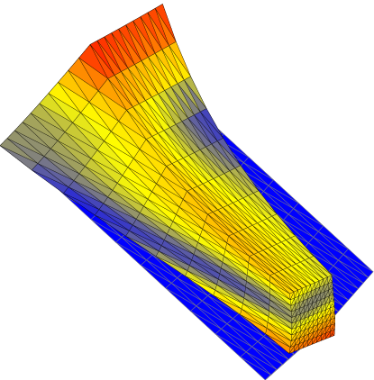
Fig. 1: Computational domain (blue) deformed by exaggerated(4x) analytical displacement used in the numerical examples. The deformed body is colored by the magnitude of the displacement.

In the final example a preconditioned CG method will be applied to solve the singular elasticity problem with data such that the compatibility conditions (2) are met.

Example 2.3.

We consider a modified problem from Example 2.2 where $f$ is not perturbed by rigid motions. As the data satisfy (2), the discrete linear system is solvable and amenable to solution by the preconditioned CG method. To this end the rigid motions are passed to the conjugate gradient solver via the PETSc interface . The mass or identity matrix is added to the singular system matrix in order to obtain a positive definite matrix in the construction of the preconditioner based on AMG. The first choice can be viewed as a simple mean to get an invertible system while the motivation for the latter is the functional setting to be discussed later in Theorem 2. Moreover, for each preconditioner two cases are considered where the converged vector is either postprocessed by removing from it the components of the nullspace or no postprocessing is applied. We note that in this example the iterations are started from a zero initial vector and the relative tolerance of $10^{-10}$ is used as a convergence criterion. The number of iterations together with error and convergence rates based on the $H^{1}$ norm are reported in Table 3. We observe that the method with the mass matrix (cf. left pane of the table) yields convergent solutions only if postprocessing is applied. On the other hand solutions with the preconditioner based on the identity matrix converge in the $H^{1}$ norm even if no postprocessing is used. The observation that the Krylov iterations/preconditioners respectively do and do not introduce rigid motions (recall that the initial guess and right hand side are orthogonal to the kernel) is related to properties of the added matrices. A vector free of rigid motions remains orthogonal after applying to it the identity matrix. This property in general does not hold for the (not diagonal) mass matrix.

Table 3: Convergence of the preconditioned CG method for the singular elasticity problem. Positive definite preconditioners using respectively the mass and identity matrices to get a nonsingular system are considered. The maximum number of iterations is set to 150. The iterations are unbounded in both cases. Solutions due to preconditioner using the identity matrix converge at nearly optimal rate.

size	AMG($\mathbf{A}+\mathbf{M}$)				AMG($\mathbf{A}+\mathbf{I}$)
	kernel not removed		kernel removed		kernel not removed		kernel removed
	$\lVert u-u_{h}\rVert_{1}$	#	$\lVert u-u_{h}\rVert_{1}$	#	$\lVert u-u_{h}\rVert_{1}$	#	$\lVert u-u_{h}\rVert_{1}$	#
2187	1.97E-02(0.26)	17	5.08E-03(0.99)	17	1.11E-02(0.87)	21	5.08E-03(0.99)	21
14739	2.58E-02(-0.39)	19	2.29E-03(1.15)	19	2.87E-03(1.95)	35	2.29E-03(1.15)	35
107811	2.80E-02(-0.12)	34	1.06E-03(1.11)	34	1.21E-03(1.24)	81	1.06E-03(1.11)	81
823875	2.82E-02(-0.01)	53	5.12E-04(1.04)	54	6.32E-04(0.94)	$>$150	5.12E-04(1.04)	$>$150

Examples 2.1–2.3 have illustrated some of the issues that might be encountered when solving the singular problem (1) with the finite element method. In particular, the following questions may be posed: (i) What is the cause of the poor convergence properties of pinpointing? (ii) What should be the order optimal preconditioner for CG? (iii) What should be the order optimal preconditioner for the Lagrange multiplier formulation?

With questions (ii) and (iii) answered in detail in the remainder of the text let us briefly comment on the first question. As will become apparent, the singular problem with a known kernel, such as (1), possesses all the information necessary to formulate a well-posed problem and a convergent numerical method. In this sense, coming up with a datum to be prescribed in the pinpointed nodes is theoretically redundant, but usually required for implementation. Further, as pointed out in [9] there are stability issues with prescribing point values of $H^{1}$ functions for $d\geq 2$. However, we have not explored settings of HypreAMG or other realizations of the preconditioner that could potentially improve convergence properties of the method in Example 2.2. In this sense the two level preconditioner of [49] is interesting as the proposed method results in bounded CG iterations even with the variationaly problematic point boundary conditions.

3 Lagrange multiplier formulation

Let $Z\subset V=\left[H^{1}(\Omega)\right]^{3}$ denote the space of rigid motions of $\Omega$, For compatible data a unique solution $u$ of (1) is required to be linearly independent of functions in $Z$. To this end a Lagrange multiplier ${p}\in Z$ is introduced which enforces orthogonality of $u$ with respect to $Z$. The constrained variational formulation of (1) seeks $u\in V,{p}\in Z$ such that

$$2\mu(\epsilon(u),\epsilon(v))+\lambda(\nabla\cdot u,\nabla\cdot v)-(p,v)=(f,v)+(h,v)_{\partial\Omega}\quad \forall v\in V,$$ (6)

$$- (u,q)=0\quad \forall{q}\in Z.$$

Equation (6) defines a saddle point problem for $(u,p)\in W$, $W=V\times Z$ satisfying

$$\mathcal{A}\begin{pmatrix}u\\ p\end{pmatrix}=\begin{pmatrix}A&B\\ B^{\prime}&\end{pmatrix}\begin{pmatrix}u\\ p\end{pmatrix}=\begin{pmatrix}l\\ 0\end{pmatrix}$$ (7)

where $l\in V^{\prime}$ such that $\langle l,v\rangle=(f,v)+(h,v)_{\partial\Omega}$ and operators $A:V\rightarrow V^{\prime}$, $B:Z\rightarrow V^{\prime}$ are defined in terms of bilinear forms

$$a(u,v)=2\mu(\epsilon(u),\epsilon(v))+\lambda(\nabla\cdot u,\nabla\cdot v)\quad\text{and}\quad b(u,q)=(u,q)$$ (8)

as $\langle Au,v\rangle=a(u,v)$ and $\langle Bq,u\rangle=-b(u,q)$. We note that in (7) operator $B^{\prime}$ is the adjoint of $B$.

Existence and uniqueness of the solution to (7) follows from the Brezzi theory [13], see also [10, ch 3.4]. The proof shall utilize the inequalities given in Lemma 1.

Lemma 1.

Let $u\in V$ arbitrary and $\omega(u)$ be the skew symmetric part of the displacement gradient $\nabla u$, i.e. $\omega(u)=\tfrac{1}{2}((\nabla u)-{(\nabla u)}^{\scalebox{0.5}{$\top$}})$. Then

$$\lVert\epsilon(u)\rVert\leq\lVert\nabla u\rVert\quad\text{and}\quad\lVert\omega(u)\rVert\leq\lVert\nabla u\rVert,$$ (9a)

$$\lVert\nabla\cdot u\rVert\leq\sqrt{3}\lVert\nabla u\rVert,$$ (9b)

$$\exists C=C(\Omega)\mbox{ such that }\lVert z\rVert_{1}\leq C\lVert z\rVert\quad\forall z\in Z.$$ (9c)

Proof.

Inequality (9a) follows from the orthogonal decomposition $\nabla u=\epsilon(u)+\omega(u)$. Inequality (9b) follows by direct calculations. To establish the final inequality we first note that (9c) clearly holds for rigid motions that are translations with constant $C=1$. To verify it for rigid rotations we consider the representation $z=Sx$ for some arbitrary skew-symmetric matrix $S\in\mathbb{R}^{3\times 3}$. Then by definition $\omega(Sx)=S$ so that $(\omega(z),\omega(z))=\lvert S\rvert^{2}\lvert\Omega\rvert$ with $\lvert S\rvert=\sqrt{{\text{tr}{({S}^{\scalebox{0.5}{$\top$}}S)}}}$ the Frobenius norm. In turn

$$\lVert z\rVert^{2}=(Sx,Sx)=\lvert S\rvert^{2}(x,x)=\frac{(x,x)}{\lvert\Omega\rvert}(\omega(z),\omega(z))=c(\Omega)\lVert\nabla z\rVert^{2},\quad c(\Omega)=\frac{(x,x)}{\lvert\Omega\rvert}$$ (10)

as $\epsilon(z)=0$. Therefore (9c) holds for all rotations. We remark that the constant $c$ in (10) is related to the moment of inertia of the body. Finally the statement follows with a constant $C(\Omega)=\sqrt{1+c(\Omega)}$ from the decomposition of any $z\in Z$ into translations and rotations. ∎

Theorem 2.

Let $f,h$ such that $l\in V^{\prime}$. Then there exists a unique solution $u\in V$, ${p}\in Z$ of (7).

Proof.

We proceed by establishing the Brezzi constants. First, the bilinear form $a$ is shown to be bounded with respect to the $\lVert\cdot\rVert_{1}$. Indeed, by Cauchy-Schwarz inequality and inequalities (9a), (9b) we have for any $u,v\in V$

$$\begin{split}a(u,v)=2\mu(\epsilon(u),\epsilon(v))+\lambda(\nabla\cdot u,\nabla\cdot v)&\leq 2\mu\lVert\epsilon(u)\rVert\lVert\epsilon(u)\rVert+\lambda\lVert\nabla\cdot u\rVert\lVert\nabla\cdot v\rVert\\ &\leq(2\mu+3\lambda)\lVert\nabla v\rVert\lVert\nabla u\rVert\leq\alpha^{*}\lVert u\rVert_{1}\lVert v\rVert_{1}\end{split}$$

with $\alpha^{*}=2\lambda+3\mu$. Ellipticity of $a$ on $Z^{\perp}=\{v\in V;(v,z)=0\,\forall z\in Z\}=\{v\in V;b(v,{p})=0\,\forall{p}\in Z\}$ follows from Korn’s inequality (5). Since $\lambda\geq 0$ by assumption

$$a(u,u)=2\mu\lVert\epsilon(u)\rVert^{2}+\lambda\lVert\nabla\cdot u\rVert^{2}\geq 2\mu\lVert\epsilon(u)\rVert^{2}\geq\alpha_{*}\lVert u\rVert^{2}_{1}\quad\forall u\in Z^{\perp},$$

with $\alpha_{*}=2\mu C$ and $C=C(\Omega)$ the constant from (5). Boundedness of $b$ with a constant $\beta^{*}=1$ follows from the Cauchy-Schwarz inequality. Finally, using (9c) we have for arbitrary $p\in Z$

$$\mathop{\operatorname*{sup}\vphantom{\operatorname*{inf}}}_{v\in V}\frac{b(v,{p})}{\lVert v\rVert_{1}}\geq\frac{(p,p)}{\lVert p\rVert_{1}}\geq\frac{\lVert p\rVert^{2}}{C\lVert p\rVert}=\frac{1}{C}\lVert p\rVert$$

so that the inf-sup condition holds with $\beta_{*}=C^{-1}$ with $C$ the constant from (9c). ∎

We remark that Theorem 2 implies that the operator $\mathcal{A}:W\rightarrow W^{\prime}$ from (7) is an isomorphism. In particular, conditions (2) need not to hold for there to exist a unique solution of (6).

In order to find the solution of the well-posed (7) numerically, conditions from Theorem 2 must hold with discrete subspaces $V_{h}$, $Z_{h}$, see [18] or [10, ch 3.4]. Typically, satisfying the discrete inf-sup condition presents an issue and requires choice of compatible finite element discretization of the involved spaces, e.g. Taylor-Hood or MINI elements [3] for the Stokes equations. For the conforming discretization $V_{h}\subset V$, $Z_{h}=Z$ the following result shows that the discrete inf-sup condition holds.

Theorem 3.

Let $Z_{h}=Z$, $V_{h}\subset V$ and $b$ the bilinear form defined in (8). Then there is a constant $\beta_{*}$ independent of $h$ such that $\mathop{\operatorname*{inf}\vphantom{\operatorname*{sup}}}_{p\in Z_{h}}\mathop{\operatorname*{sup}\vphantom{\operatorname*{inf}}}_{v\in V_{h}}\tfrac{b(v,{p})}{\lVert v\rVert_{1}\lVert p\rVert}\geq\beta_{*}$.

Proof.

The proof mirrors the continuous inf-sup condition in Theorem 2. Let $p\in Z_{h}$ be given. Since $Z=Z_{h}\subset V_{h}$ we get by taking $v=p$

$$\mathop{\operatorname*{sup}\vphantom{\operatorname*{inf}}}_{v\in V_{h}}\frac{b(v,{p})}{\lVert v\rVert_{1}}\geq\frac{(p,p)}{\lVert p\rVert_{1}}\geq\frac{\lVert p\rVert^{2}}{C\lVert p\rVert}=\frac{1}{C}\lVert p\rVert,$$

where $C$ is the constant from (9c). ∎

Following Theorems 2, 3 and operator preconditioning [39, 34] the Riesz map $\mathcal{B}_{1}:W^{\prime}\rightarrow W$ with respect to inner product $(u,v)_{1}+(p,q)$ with $(u,p),(v,q)\in W$

$$\mathcal{B}_{1}={\begin{pmatrix}H&\\ &I\end{pmatrix}}^{-1},\quad H:V\rightarrow V^{\prime},\langle Hu,v\rangle=(u,v)_{1}\quad\text{and}\quad I:Z\rightarrow Z^{\prime},\langle Ip,q\rangle=(p,q)$$ (11)

defines a preconditioner for discretized (7) whose condition number is independent of $h$. This follows from Brezzi constants in Theorems 2, 3 being free of the discretization parameter.

Since applying the preconditioner (11) requires an inverse of the $6\times 6$ mass matrix of the space rigid motions it is advantageous to chose a basis of $Z$ in which the matrix is well-conditioned. With the choice of an $L^{2}$ orthonormal basis the obtained mass matrix is an identity and we shall therefore briefly discuss construction of such a basis.

3.1 Construction for orthonormal basis of rigid motions

Consider a unit cube $\Omega=\left[-\tfrac{1}{2},\tfrac{1}{2}\right]^{3}$ centered at the origin. Denoting ${e}_{i}$, $i=1,2,3$ the canonical unit vectors the set

$$Z_{\mbox{\mancube}}=\{{e}_{1},{e}_{2},{e}_{3},x\times{e}_{1},x\times{e}_{2},x\times{e}_{3}\}$$

constitutes an orthonormal basis of the rigid motions of $\Omega$ with respect to the $L^{2}$ inner product. Clearly, the basis for an arbitrary body can be obtained from $Z_{\mbox{\mancube}}$ by a Gram-Schmidt process. However, we shall advocate here a construction derived from physical considerations. The construction was originally presented by the authors in [30].

Lemma 4.

Let ${c}={\lvert\Omega\rvert}^{-1}(x,1)$ be the center of mass of $\Omega$, $I_{\Omega}$ the tensor of inertia [22, ch 4.] of $\Omega$ with respect to $c$

$$I_{\Omega}=\int_{\Omega}I{(x-{c})}^{\scalebox{0.5}{$\top$}}(x-{c})+(x-{c})\otimes(x-{c})\,\mathrm{d}x$$

and $(\lambda_{i},{v}_{i})$, $i=1,2,3$ the eigenpairs of the tensor. Then the set

$$Z_{\Omega}=\{\lvert\Omega\rvert^{\scalebox{0.5}{$-\tfrac{1}{2}$}}v_{1},\lvert\Omega\rvert^{\scalebox{0.5}{$-\tfrac{1}{2}$}}v_{2},\lvert\Omega\rvert^{\scalebox{0.5}{$-\tfrac{1}{2}$}}v_{3},\lambda_{1}^{\scalebox{0.5}{$-\tfrac{1}{2}$}}(x-{c})\times v_{1},\lambda_{2}^{\scalebox{0.5}{$-\tfrac{1}{2}$}}(x-{c})\times v_{2},\lambda_{3}^{\scalebox{0.5}{$-\tfrac{1}{2}$}}(x-{c})\times v_{3}\}$$ (12)

is the $L^{2}$ orthonormal basis of rigid motions of $\Omega$.

Proof.

Note that by construction $I_{\Omega}$ is a symmetric positive definite tensor. Thus $\lambda_{i}>0$ and there exists a complete set of eigenvectors ${v_{i}}^{\scalebox{0.5}{$\top$}}v_{j}=\delta_{ij}$. We proceed to show that the Gram matrix of the proposed basis is an identity. First $(v_{i},v_{j})=\lvert\Omega\rvert\delta_{ij}$ by orthonormality of the eigenvectors. Further, for $((x-c)\times v_{i},v_{j})=(v_{i}\times v_{j},(x-c))$ and in the nontrivial case $i\neq j$ the product is zero since $c$ is the center of mass. Finally $((x-{c})\times v_{i},(x-{c})\times v_{j})={v_{i}}^{\scalebox{0.5}{$\top$}}I_{\Omega}v_{j}=\lambda_{i}\delta_{ij}$. ∎

We remark that the rigid motions of the body are in the constructed basis given in terms of translations along and rotations around the principal axes of the tensor that describes its rotational kinetic energy.

Note also, that the construction can be generalized to yield an orthonormal basis with respect to different inner products. In particular, let $Z_{h}=\operatorname{span}{\{z_{k}\}_{k=1}^{6}}\subset V_{h}$ be functions approximating some basis of $Z$. For $u,v\in V_{h}$ let $\mathbf{u}=\pi_{h}u$, $\mathbf{v}=\pi_{h}v$ be coefficient vectors in the nodal basis of $V_{h}$. The $l^{2}$ orthonormal basis of $Z_{h}$ can be created using Lemma 4 by replacing $(u,v)$ with ${\mathbf{u}}^{\scalebox{0.5}{$\top$}}\mathbf{v}$. The differences between the bases are shown in Figure 2 where the defining principal axes of the $L^{2}$ and $l^{2}$ orthonormal basis of rigid motions are drawn. If $\Omega$ is uniformly triangulated the bases are practically identical. However, the $l^{2}$ basis changes in the presence of a non-uniform mesh refinement.

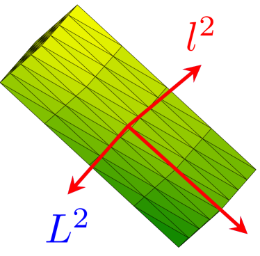
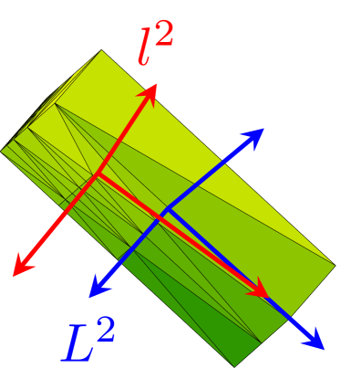
Fig. 2: Computational domains considered in the numerical examples for linear elasticity are obtained by uniformly refining the parent mesh. (Left) Parent is close to uniformly triangulated. (Right) The parent mesh is refined near a single edge of the domain. The blue and red arrows indicate the principal axes of the tensor $I_{\Omega}$, cf. Lemma 4, defined using the $L^{2}$ and $l^{2}$ inner products. Axes are drawn from the center of mass computed using the respected inner products. Only the $L^{2}$ basis is stable upon change of triangulation from uniform (left) to nonuniform (right).

Formulation of the problem (6) with respect to an $L^{2}$ orthonormal basis $\{z_{k}\}_{k=1}^{6}$ of the space of rigid motions results in the mapping between $Z$ and $\mathbb{R}^{6}$ being an isometry. In turn, if the discretized problem is considered with space $V_{h}\times\mathbb{R}^{6}$ and its natural norm, the Brezzi constants will be those obtained in Theorem 3. On the other hand, for a non-orthonormal basis only equivalence between the norms holds: There exists $C_{1},C_{2}>0$ such that for all $p\in Z$

$$C_{1}\lvert c\rvert\leq\lVert p\rVert\leq C_{2}\lvert c\rvert,\quad p=\sum_{k=1}^{6}c_{k}z_{k}$$

and the constants $C_{1},C_{2}$ enter the estimates in the Brezzi theory. For an unfortunate choice of the basis it is then possible that $C_{1}=C_{1}(h)$ or $C_{2}=C_{2}(h)$ leading to mesh dependent performance of a preconditioner using the $l^{2}$ norm for (the Lagrange multiplier space) $\mathbb{R}^{6}$.

Returning to preconditioner (11) recall that the Brezzi constants $\alpha^{*},\alpha_{*}$ depend on the Lamé constants and thus $\mathcal{B}_{1}$ does not define a parameter robust preconditioner. To address the dependence on material parameters, we shall at first assume that $\mu$ and $\lambda$ are comparable in magnitude. The case $\lambda\gg\mu$ is postponed until §6.

3.2 Robust preconditioning of the singular problem

Parameter robust preconditioners for the Lagrange multiplier formulation of the singular elasticity problem (6) can be analyzed by the operator preconditioning framework of [39]. The preconditioners are constructed by considering (7) in parameter dependent spaces, e.g. [8], which are equivalent with $V$ as a set, but the topology of the spaces is given by different, parameter dependent, norms. Two such norms leading to two different preconditioners are constructed next.

For $u\in V$ consider the orthogonal decomposition $u=u_{Z}+u_{Z^{\perp}}$ where $u_{z}\in Z$ and $u_{z^{\perp}}\in Z^{\perp}$. Bilinear forms $(\cdot,\cdot)_{E}$, $(\cdot,\cdot)_{M}$ over $V$ are defined in terms of $A$ from (7) and operators $Y:V\rightarrow V^{\prime}$, $M:V\rightarrow V^{\prime}$ as

$$\langle Yu,v\rangle=(u_{Z},v_{Z}), \quad\quad(u,v)_{E}=\langle Au,v\rangle+\langle Yu,v\rangle,$$ (13)

$$\langle Mu,v\rangle=(u,v), \quad\quad(u,v)_{M}=\langle Au,v\rangle+\langle Mu,v\rangle.$$

The forms (13) define functionals $\lVert\cdot\rVert_{E}$ and $\lVert\cdot\rVert_{M}$ over $V$ such that

$$\lVert u\rVert_{E}=\sqrt{(u,u)_{E}}\quad\text{and}\quad\lVert u\rVert_{M}=\sqrt{(u,u)_{M}}.$$ (14)

Lemma 5.

Let $\lVert\cdot\rVert_{E}$ and $\lVert\cdot\rVert_{M}$ be the functionals (14). Then $\lVert\cdot\rVert_{E}$ and $\lVert\cdot\rVert_{M}$ define norms on $V$ which are equivalent with the $H^{1}$ norm.

Proof.

From the orthogonal decomposition of $u\in V$ it follows that $\lVert u\rVert^{2}_{M}=\lVert u\rVert^{2}_{E}+\lVert u_{Z^{\perp}}\rVert^{2}$. Together with Lemma 1 we thus establish

$$\lVert u\rVert^{2}_{E}\leq\lVert u\rVert^{2}_{M}\leq(2\mu+3\lambda+1)\lVert u\rVert^{2}_{1}\quad\forall u\in V.$$

To complete the equivalence, let $C=C(\Omega)$ be the constant from Korn’s inequality (4). Then for all $u\in V$

$$\lVert u\rVert^{2}_{M}\geq 2\mu\lVert\epsilon(u)\rVert^{2}+\lVert u\rVert^{2}\geq c\lVert u\rVert^{2}_{1},$$

with $c=C$ for $2\mu>1$ and $c=2\mu C$ otherwise. Finally, for equivalence of the $E$-norm, the Korn’s inequality on $Z^{\perp}$, see (5) also Theorem 2, yields

$$\lVert u\rVert^{2}_{E}=2\mu\lVert\epsilon(u)\rVert^{2}+\lambda\lVert\nabla\cdot u\rVert^{2}\geq 2\mu C\lVert u\rVert^{2}_{1}\quad\forall u\in Z^{\perp}$$

with $C=C(\Omega)$, while using (9c) in Lemma 1 gives

$$\lVert u\rVert_{E}=\lVert u\rVert\geq C_{1}(\Omega)\lVert u\rVert_{1}$$

for any $u\in Z$. Thus $E$ and $H^{1}$ norms are equivalent on $Z^{\perp}$ and $Z$ respectively. The proof is completed by observing that $u_{Z}$ and $u_{Z^{\perp}}$ satisfy $(u_{Z},u_{Z^{\perp}})_{E}=0$ so that

$$\begin{split}\lVert u\rVert^{2}_{E}=2\mu\lVert\epsilon(u_{Z^{\perp}})\rVert^{2}+\lambda\lVert\nabla\cdot u_{Z^{\perp}}\rVert^{2}+\lVert u_{Z}\rVert^{2}&\geq 2\mu C\lVert u_{Z^{\perp}}\rVert^{2}_{1}+C_{1}\lVert u_{Z}\rVert^{2}_{1}\\ &\geq c(\lVert u_{Z^{\perp}}\rVert^{2}_{1}+\lVert u_{Z}\rVert^{2}_{1}),\end{split}$$

$c=\min(2\mu C,C_{1})$, while for the $H^{1}$ inner product $\lVert u\rVert^{2}_{1}\leq 2(\lVert u_{Z^{\perp}}\rVert^{2}_{1}+\lVert u_{Z}\rVert^{2}_{1})$ holds. Thus $\lVert u\rVert_{E}^{2}\geq\tfrac{c}{2}\lVert u\rVert_{1}^{2}$ for all $u\in V$. ∎

Using equivalent norms of $V$ from Lemma 5 we readily establish equivalent norms for the product space $W=V\times Z$

$$\lVert w\rVert_{E}=\lVert(u,p)\rVert_{E}=\sqrt{\lVert u\rVert_{E}^{2}+\lVert p\rVert^{2}}\quad\text{and}\quad\lVert w\rVert_{M}=\lVert(u,p)\rVert_{M}=\sqrt{\lVert u\rVert_{M}^{2}+\lVert p\rVert^{2}}$$ (15)

and consider as preconditioners for (7) the operators $\mathcal{B}_{E}:W^{\prime}\rightarrow W$ and $\mathcal{B}_{M}:W^{\prime}\rightarrow W$

$$\mathcal{B}_{E}={\begin{pmatrix}A+Y&\\ &I\end{pmatrix}}^{-1}\quad\text{and}\quad\mathcal{B}_{M}={\begin{pmatrix}A+M&\\ &I\end{pmatrix}}^{-1}.$$ (16)

Note that the mappings (16) are the Riesz maps with respect to the inner products which induce norms (15). We proceed with analysis of the properties of $\mathcal{B}_{E}$.

Theorem 6.

Let $\mathcal{A}:W\rightarrow W^{\prime}$ be the operator and the space from (7) and $W_{E}$ be the space $W$ considered with $\lVert\cdot\rVert_{E}$ norm (15). Then $\mathcal{A}:W_{E}\rightarrow W_{E}^{\prime}$ is an isomorphism. Moreover the Riesz map $\mathcal{B}_{E}:W_{E}^{\prime}\rightarrow{W_{E}}$ in (16) defines the canonical preconditioner for (7).

Proof.

We shall show that the first assertion holds by establishing the Brezzi constants. Recall the definition of the bilinear form $a$ given in (8). Then, by the Cauchy-Schwarz inequality and (9a) in Lemma 1, the inequality $a(u,v)\leq\sqrt{a(u,u)}\sqrt{a(v,v)}$ holds for any $u,v\in V$. In turn for all $u,v\in V$

$$a(u,v)\leq\sqrt{a(u,u)}\sqrt{a(v,v)}\leq\sqrt{a(u,u)+(u_{Z},u_{Z})}\sqrt{a(v,v)+(v_{Z},v_{Z})}=\lVert u\rVert_{E}\lVert v\rVert_{E}$$

and $a$ is bounded with respect to $E$ norm with a constant $\alpha^{*}=1$. Further, $u_{Z}=0$ for $u\in Z^{\perp}$. Hence $a(u,u)=a(u,u)+(u_{Z},u_{Z})=\lVert u\rVert^{2}_{E}$ for all $u\in Z^{\perp}$ and the form is $E$ elliptic on $Z^{\perp}$ with constant $\alpha^{*}=1$. To compute the boundedness constant of the form $b$, the orthogonal decomposition $u=u_{Z}+u_{Z^{\perp}}$ is used so that for all $u\in V$, $q\in Z$

$$b(u,q)=(u_{Z}+u_{Z^{\perp}},q)=(u_{Z},q)\leq\lVert u_{Z}\rVert\lVert q\rVert=\sqrt{a(u,u)+\lVert u_{Z}\rVert^{2}}\lVert q\rVert=\lVert u\rVert_{E}\lVert q\rVert$$

and we have $\beta^{*}=1$. Finally, taking any $q\in Z$ and setting $u=q$ in

$$\mathop{\operatorname*{sup}\vphantom{\operatorname*{inf}}}_{u\in V}\frac{b(u,{q})}{\lVert u\rVert_{E}}\geq\frac{(q,q)}{\sqrt{a(q,q)+(q_{Z},q_{Z})}}=\frac{\lVert q\rVert^{2}}{\sqrt{0+\lVert q\rVert^{2}}}\geq\lVert q\rVert$$

and thus the inf-sup condition holds with $\beta_{*}=1$. As all the constants are independent of material parameters, the second assertion follows from the first one by operator preconditioning [39, ch 5.]. ∎

Using Theorem 6 it is readily established that the condition number of the composed operator $\mathcal{B}_{E}\mathcal{A}:W\mapsto W$ is equal to one. We further note that discretizing operator $\mathcal{B}_{E}$ leads to discrete nullspace preconditioners of [7, ch 6.].

While the spectral properties of $\mathcal{B}_{E}$ are appealing, the preconditioner is impractical. Consider $\mathbf{B}_{E}$ as a matrix representation of the Galerkin approximation of $\mathcal{B}_{E}$ in $W_{h}\subset W$. Then $\mathbf{B}_{E}={\text{diag}(\mathbf{A}+\mathbf{Y}{\mathbf{Y}}^{\scalebox{0.5}{$\top$}},\mathbf{I})}^{-1}$ where $\mathbf{Y}=\mathbb{R}^{n\times 6}$, $\mathbf{y}_{k}=\text{col}_{k}\mathbf{Y}=\pi_{h}z_{k}$ and $z_{k}\in V_{h}$ is the function from the $L^{2}$ orthogonal basis of the space of rigid motions. Due to the second (nonlocal) term the matrix $\mathbf{A}+\mathbf{Y}{\mathbf{Y}}^{\scalebox{0.5}{$\top$}}$ is dense. Further, as shall be discussed in §4, inverting the operator requires computing (the action of) the pseudoinverse of the singular matrix $\mathbf{A}$. The mapping $\mathcal{B}_{M}$, on the other hand, leads to a more practical preconditioner.

Theorem 7.

Let $\mathcal{A}:W\rightarrow W^{\prime}$ be the operator and space defined in (7) and $W_{M}$ be defined analogically to Theorem 6. Then $\mathcal{A}:W_{M}\rightarrow W_{M}^{\prime}$ is an isomorphism. Moreover the Riesz map $\mathcal{B}_{M}:W_{M}^{\prime}\rightarrow W_{M}$ in (16) defines a parameter robust preconditioner for (7).

Proof.

As in the proof of Theorem 6 we establish that $a(u,v)\leq\lVert u\rVert_{M}\lVert v\rVert_{E}$ for all $u,v\in V$ and $b(v,p)\leq\lVert v\rVert\lVert p\rVert\leq\lVert v\rVert_{M}\lVert p\rVert$ for all $v\in V$, $p\in Z$. Setting $v=p\in Z$ then yields $\mathop{\operatorname*{inf}\vphantom{\operatorname*{sup}}}_{p\in Z}\mathop{\operatorname*{sup}\vphantom{\operatorname*{inf}}}_{v\in V}\tfrac{b(v,p)}{\lVert v\rVert_{M}\lVert p\rVert}\geq 1$. For $M$ ellipticity of $a$ on $Z^{\perp}$, assume existence of $C=C(\Omega)$ such that $\lVert u\rVert^{2}\leq C\lVert\epsilon(u)\rVert^{2}$ for all $u\in Z^{\perp}$. Then on $Z^{\perp}$

$$\lVert u\rVert^{2}\leq C\lVert\epsilon(u)\rVert^{2}\leq C\mu\lVert\epsilon(u)\rVert^{2}\leq C(2\mu\lVert\epsilon(u)\rVert^{2}+\lambda\lVert\nabla\cdot u\rVert^{2})=C\lVert u\rVert^{2}_{E}$$

and

$$\lVert u\rVert^{2}_{M}=\lVert u\rVert^{2}_{E}+\lVert u\rVert^{2}\leq(C+1)\lVert u\rVert^{2}_{E}$$

so that $a(u,u)=\lVert u\rVert^{2}_{E}\geq{(1+C)}^{-1}\lVert u\rVert^{2}_{M}$. Finally we comment on the assumption of existence of the constant $C$. Assume the contrary. Then there is $u\in Z^{\perp}$ such that $\lVert e(u)\rVert=1$, $\lVert w(u)\rVert=0$ and the $\lVert u\rVert$ unbounded. However, such $u$ violates Korn’s inequality (5). ∎

We remark that Theorem 7 required an additional assumption $2\mu\geq 1$. The assumption is not restrictive as it can be always achieved by scaling the equations such that the inequality is satisfied. Note also that with the orthonormal basis of rigid motions the discrete preconditioner based on $\mathcal{B}_{M}$ is such that ${\mathbf{B}_{M}}^{-1}=\text{diag}(\mathbf{A}+\mathbf{M},\mathbf{I})$, with $\mathbf{M}$ the mass matrix. The system to be assembled is therefore sparse.

Following Theorem 7 the condition number of the preconditioned operator $\mathcal{B}_{M}\mathcal{A}:W\rightarrow W$ depends solely on the constant $C$ from Korn’s inequality (5). An approximation for the constant is provided by the smallest positive eigenvalue $\lambda^{+}_{\text{min}}$ of the problem

$$\begin{pmatrix}\mathbf{A}&\mathbf{B}\\ {\mathbf{B}}^{\scalebox{0.5}{$\top$}}&\end{pmatrix}\begin{pmatrix}\mathbf{u}\\ \mathbf{p}\end{pmatrix}=\lambda\begin{pmatrix}\mathbf{A}+\mathbf{M}&\\ &\mathbf{I}\end{pmatrix}\begin{pmatrix}\mathbf{u}\\ \mathbf{p}\end{pmatrix}.$$

In Table 10, Appendix A, the constant has been computed for two different domains; a cube from Example 2.2 and a hollow cylinder. In both cases $C\approx 1$ can be observed.

In order to demonstrate $h$ robust properties of $\mathcal{B}_{M}$, the problem from Example 2.2 is considered with basis from §3.1 and discretized on $V_{h}\subset V$. The resulting preconditioned linear system is solved by the minimal residual (MinRes) method [41] as implemented in cbc.block, the FEniCS library for block matrices [36] using as the preconditioner

$$\mathbf{B}_{M}=\begin{pmatrix}\text{AMG}(\mathbf{A}+\mathbf{M})&\\ &\mathbf{I}\end{pmatrix}.$$

More specifically, the preconditioner uses a single AMG $V$ cycle with one pre and post smoothing by a symmetric SOR smoother. The rigid motions were not passed to the routine on initialization. The saddle point system was assembled and invertedusing cbc.block. The results of the experiment are presented in Table 5. Clearly, the number of iterations required for convergence is independent of the discretization. Moreover, the method yields numerical solutions which converge in the $H^{1}$ norm at the optimal rate on both the uniform and nonuniform meshes, cf. Figure 2.

A drawback of the Lagrange multiplier formulation is the cost of solving the resulting indefinite linear system. Following e.g. [20, ch 7.2] let the condition number of a Hermitian matrix $\mathbf{A}$ be $\kappa(\mathbf{A})=\nicefrac{{\lambda_{\text{max}}(\mathbf{A})}}{{\lambda_{\text{min}}(\mathbf{A})}}$ where $\lambda_{\text{max}}(\mathbf{A})$, $\lambda_{\text{min}}(\mathbf{A})$ are respectively the largest and smallest (in magnitude) eigenvalues of the matrix. For $\mathbf{A}$ Hermitian indefinite and under simplifying assumptions on the spectrum [32, ch 3.2] gives the following bound on the relative error in residual $r_{n}$ at step $n$ of the MinRes method

$$\frac{\lvert r_{n}\rvert}{\lvert r_{0}\rvert}\leq 2\left(\frac{\kappa(\mathbf{A})-1}{\kappa(\mathbf{A})+1}\right)^{\lfloor n/2\rfloor}.$$

The result should be contrasted with a similar one for the error $e_{n}$ at the $n$-th step of CG method on symmetric positive definite matrix $\mathbf{A}$, e.g. [48, thm 38.5],

$$\frac{{e_{n}}^{\scalebox{0.5}{$\top$}}\mathbf{A}e_{n}}{{e_{0}}^{\scalebox{0.5}{$\top$}}\mathbf{A}e_{0}}\leq 2\left(\frac{\sqrt{\kappa(\mathbf{A})}-1}{\sqrt{\kappa(\mathbf{A})}+1}\right)^{n}.$$

While the above estimates are known to give the worst case behavior of the two methods, the faster rate of convergence of CG motivates investigating formulations of (1) to which the conjugate gradient method can be applied.

4 Conjugate gradient method for discrete singular problems

We consider a variational formulation of (1): Find $u\in V=\left[H^{1}(\Omega)\right]^{3}$ such that

$$2\mu(\epsilon(u),\epsilon(v))+\lambda(\nabla\cdot u,\nabla\cdot v)=(f,v)+(h,v)_{\partial\Omega}\quad\forall v\in V.$$ (17)

Denoting $a:V\times V\rightarrow\mathbb{R},l:V^{\prime}\rightarrow\mathbb{R}$ the bilinear and linear forms defined by (17), we note that the problem is not well-posed in $V$. Indeed, the compatibility conditions (2) restrict the functionals for which the solution can be found to $l\in Z^{0}=\{f\in V^{\prime};\langle f,z\rangle=0\,\forall z\in Z\}$. Moreover, only the part of $u$ in $Z^{\perp}$ is uniquely determined by (17). More precisely we have the following result.

Theorem 8.

Let $l\in Z^{0}$. Then there exists a unique solution of the problem

$$\text{Find }u\in Z^{\perp}\text{ such that for any }v\in Z^{\perp}\text{ it holds that }a(u,v)=\langle l,v\rangle.$$ (18)

Proof.

The complete proof can be found as Theorem 11.2.30 in [11]. Note that boundedness and ellipticity of $a$ on $Z^{\perp}$ with $\lVert\cdot\rVert_{1}$ are proven as part of Theorem 2. ∎

We remark that if (2) holds then $u\in Z^{\perp}$ solves (18) if and only if $(u,0)$ solves the Lagrange multiplier problem (7). Further, the well-posed variational problem (18) is not suitable for discretization by the finite element method as the approximation leads to a dense linear system. A sparse discrete problem to which the conjugate gradient method shall be applied is therefore derived from (17).

Recall $\dim{Z}=6$, $n=\dim{V_{h}}$ and let $V_{h}=\operatorname{span}{\{\phi_{i}\}_{i=1}^{n}}$. Discretizing the variational problem (17) leads to a linear system

$$\mathbf{A}\mathbf{u}=\mathbf{b},$$ (19)

where $\mathbf{A}\in\mathbb{R}^{n\times n}$ such that $A_{ij}=a(\phi_{j},\phi_{i})$ and vector $\mathbf{b}\in\mathbb{R}^{n}$, $b_{i}=\langle l,\phi_{i}\rangle$. Note that we shall consider (19) for a general right hand side, that is, not necessarily a discretization of $l\in Z^{0}$. We proceed by reviewing properties of the discrete system.

Due to symmetry and ellipticity of the bilinear form $a$ on $Z^{\perp}$ there exists respectively $6$ vectors $\mathbf{z}_{k}$ and $n-6$ eigenpairs $(\gamma_{i},\mathbf{u}_{i})$, $\gamma_{i}>0$ such that $\mathbf{A}\mathbf{z}_{k}=0$, ${\mathbf{z}_{k}}^{\scalebox{0.5}{$\top$}}\mathbf{u}_{i}=0$, $\mathbf{A}\mathbf{u}_{i}=\gamma_{i}\mathbf{u}_{i}$ and ${\mathbf{u}_{i}}^{\scalebox{0.5}{$\top$}}\mathbf{u}_{j}=\delta_{ij}$. From the decomposition of $\mathbf{A}$ it follows that the system (19) is solvable if and only if ${\mathbf{z}_{k}}^{\scalebox{0.5}{$\top$}}\mathbf{b}=0$ for any $k$ and the unique solution of the system is $\mathbf{u}\in\operatorname{span}{\{\mathbf{u}_{i}\}_{i=1}^{n-6}}$. We note that the last statement is the Fredholm alternative for (19). As a further consequence of the decomposition it is readily verified that given compatible vector $\mathbf{b}$, the solution of (19) is $\mathbf{u}=\mathbf{B}_{A}\mathbf{b}$ with $\mathbf{B}_{A}$ such that $\mathbf{B}_{A}\mathbf{y}=\sum_{i}{\gamma_{i}}^{-1}\left({\mathbf{u}_{i}}^{\scalebox{0.5}{$\top$}}\mathbf{y}\right)\mathbf{u}_{i}$. The matrix $\mathbf{B}_{A}$ is the pseudoinverse [42] or natural inverse [31, ch 3.] of $\mathbf{A}$.

We note that any vector from $\mathbb{R}^{n}$ can be orthogonalized with respect to the kernel of $\mathbf{A}$ by a projector $\mathbf{P}_{Z}=\mathbf{I}-\mathbf{Z}{\mathbf{Z}}^{\scalebox{0.5}{$\top$}}$, where $\mathbf{Z}\in\mathbb{R}^{n\times 6}$ is the matrix consisting of $l^{2}$ orthonormal basis vectors of the kernel.

With $\mathbf{b}$ such that ${\mathbf{Z}}^{\scalebox{0.5}{$\top$}}\mathbf{b}=0$ the solution $\mathbf{u}$ of linear system (19) can be computed by the conjugate gradient method, e.g. [45]. Let $\mathbf{u}^{0}$ be the starting vector for the iterations. Then, assuming exact arithmetic and no preconditioner, the method preserves the component of $\mathbf{u}^{0}$ in $\mathbf{Z}$, i.e. ${\mathbf{Z}}^{\scalebox{0.5}{$\top$}}\mathbf{u}^{0}={\mathbf{Z}}^{\scalebox{0.5}{$\top$}}\mathbf{u}$. In particular, ${\mathbf{Z}}^{\scalebox{0.5}{$\top$}}\mathbf{u}^{0}=0$ is required to obtain a solution orthogonal to the kernel. On the other hand, let $\mathbf{B}$ be the CG preconditioner. Then the iterations introduce components of the kernel to the solution even if ${\mathbf{Z}}^{\scalebox{0.5}{$\top$}}\mathbf{u}^{0}=0$, unless the range of $\mathbf{B}$ is orthogonal to $\mathbf{Z}$.

4.1 Preconditioned CG for singular elasticity problem

A suitable preconditioner for (19) is obtained by a composition with the $\mathbf{P}_{Z}$ projector and we shall consider $\mathbf{B}_{M}=\mathbf{P}_{Z}{(\mathbf{A}+\mathbf{M})}^{-1}$ where $\mathbf{M}$ is the mass matrix. That the preconditioner leads to bounded iteration count (and converging numerical solutions) is demonstrated in Table 4, cf. left pane. The preconditioner is also compared with a different preconditioner based on the approximation of the pseudoinverse $\mathbf{B}_{A}$. The approximation can be constructed by passing a kernel of the operator to the CG routine, in the form of the $l^{2}$ orthonormal basis vectors, see MatSetNullSpace in PETSc[5]. Note that the preconditioners perform similarly in terms of iteration count, however, for large systems the pseudoinverse appears to be a faster method.

We remark that in terms of operator preconditioning, the preconditioner based on the pseudoinverse can be interpreted as a Riesz map $Z^{0}\rightarrow Z^{\perp}$ defined with respect to the inner product induced by the bilinear form $a$. Recall that $a$ is symmetric and elliptic on $Z^{\perp}$. On the other hand $\mathbf{B}_{M}$ approximates a mapping $Z^{0}\rightarrow V\rightarrow Z^{\perp}$.

Table 4: Preconditioned CG iterations on (19) obtained by discretization of (17) with problem parameters as in Example 2.2 and two preconditioners. Both systems are solved with relative tolerance of $10^{-10}$. Uniform mesh is used.

size	$\mathbf{P}_{z}\text{AMG}(\mathbf{A}+\mathbf{M})$			$\text{AMG}(\mathbf{A}|\mathbf{Z})$
	$\lVert u-u_{h}\rVert_{1}$	#	time $\left[s\right]$	$\lVert u-u_{h}\rVert_{1}$	#	time $\left[s\right]$
14739	1.14E-02 (1.09)	22	0.491	1.14E-02 (1.09)	21	0.537
107811	5.49E-03 (1.06)	23	10.17	5.49E-03 (1.06)	23	10.96
823875	2.71E-03 (1.02)	24	103.5	2.71E-03 (1.02)	25	86.51
6440067	1.35E-03 (1.00)	26	1580	1.35E-03 (1.00)	26	911.9

Having established preconditioners for the indefinite system stemming from the Lagrange multiplier formulation (7) and the positive semi-definite problem stemming from (17), we shall finally discuss approximation properties of the computed solutions. To this end the problem from Example 2.2 is considered where $f$ is perturbed by rigid motions. Note that while with the new functional $l$ the problem (7) is well-posed, in (19) a compatible right hand side $\mathbf{b}$ will be obtained by projector $\mathbf{P}_{Z}$.

Results of the experiment are listed in Table 5. The Lagrange multiplier method converges at optimal rate on both uniformly and non-uniformly discretized mesh, cf. Figure 2. On the other hand, solutions to (19) converge to the true solution only on the uniform mesh while there is no convergence with nonuniform discretization. Note that this is not signaled by growth of the iterations - for both methods the iteration counts are bounded. Note also that MinRes takes about twice as many iterations as CG.

Table 5: (top) Convergence properties of the Lagrange multiplier formulation (7) and (bottom) the singular formulation (17) utilizing $l^{2}$ orthogonal basis of the nullspace to invert the system (19). Only the multiplier formulation yields solutions converging on uniform and nonuniform meshes. Relative tolerances of $10^{-11}$ and $10^{-10}$ are used for MinRes and CG respectively.

uniform				refined
size	$\lVert u-u_{h}\rVert_{1}$	#	$\max_{Z}|(u_{h},z)|$	size	$\lVert u-u_{h}\rVert_{1}$	#	$\max_{Z}|(u_{h},z)|$
14745	1.03E-02 (1.14)	44	3.54E-07	13080	3.11E-02 (0.99)	50	1.68E-07
107817	4.84E-03 (1.09)	45	2.77E-06	98052	1.41E-02 (1.14)	53	6.73E-08
823881	2.36E-03 (1.03)	45	1.38E-06	759546	6.53E-03 (1.11)	54	8.11E-07
6440073	1.18E-03 (1.00)	44	1.75E-05	5978835	3.20E-03 (1.03)	55	2.94E-06
14739	1.14E-02 (1.09)	21	1.30E-03	13074	5.51E-02 (0.45)	26	6.06E-03
107811	5.49E-03 (1.06)	23	6.66E-04	98046	5.05E-02 (0.12)	27	6.32E-03
823875	2.71E-03 (1.02)	25	3.36E-04	759540	5.00E-02 (0.02)	29	6.43E-03
6440067	1.35E-03 (1.00)	26	1.69E-04	5978829	4.98E-02 (0.01)	31	6.49E-03

From the experiment we conclude that the conjugate gradient method for (19), as applied so far, in general does not yield converging numerical solutions of (17). It is next shown that the issue is due projector $\mathbf{P}_{Z}=\mathbf{I}-\mathbf{Z}{\mathbf{Z}}^{\scalebox{0.5}{$\top$}}$ which the method uses and which is derived from the discrete problem. In particular, we show that $\mathbf{P}_{Z}$ is not a correct discretization of a projector used in the continuous problem (18) (and (7)). Following the continuous problem, a modification to CG is proposed, which leads to a converging method.

4.2 Conjugate gradient method with $Z^{0}$, $Z^{\perp}$ projectors

Consider the variational problem (18) which was proven well-posed in Theorem 8 under the assumptions $l\in Z^{0}\subset V^{\prime}$ and $u\in Z^{\perp}\subset V$. In this respect, there are two subspaces associated with (18) and we shall define two projectors $P:V\rightarrow Z^{\perp}$, $P^{\prime}:V^{\prime}\rightarrow Z^{0}$ such that for $u\in V$, $f\in V^{\prime}$

$$(Pu,v)=(u_{Z^{\perp}},v)\quad\forall v\in V,$$ (20)

$$\langle P^{\prime}f,u\rangle=\langle f,u-u_{z}\rangle.$$

Similar projectors were discussed in [9] for the singular Poisson problem. We note that $\langle f,Pu\rangle=\langle P^{\prime}f,u\rangle$ and thus $P^{\prime}$ is the adjoint of $P$.

Lemma 9.

Let $l\in V^{\prime}$ and $P,P^{\prime}$ be the projectors (20). Then $(u,p)\in V\times Z$ solves (7) with the right hand side $(v,q)\mapsto\langle l,v\rangle+\langle 0,q\rangle$ if and only if $u\in Z^{\perp}$ and $u$ solves (18) with the right hand side $P^{\prime}l$.

Proof.

It suffices to establish the relation between the right hand sides. Testing (7) with $(z,0)$, $z\in Z$ yields that $(p,z)=\langle l,z\rangle$. In turn we have for any $v\in V$

$$\langle l,v\rangle-(p,v)=\langle l,v\rangle-(p,v_{Z}+v_{Z^{\perp}})=\langle l,v\rangle-\langle l,v_{Z}\rangle=\langle l,v-v_{Z}\rangle=\langle l,Pv\rangle$$

and the new right hand side of (7) is therefore $(v,q)\mapsto\langle P^{\prime}l,v\rangle+\langle 0,q\rangle$. ∎

To derive a matrix representation of the projectors with respect to nodal basis $V_{h}=\operatorname{span}{\{\phi_{i}\}_{i=1}^{n}}$, the mappings $\pi_{h}:V_{h}\rightarrow\mathbb{R}^{n}$ (the nodal interpolant) and $\mu_{h}:V^{\prime}_{h}\rightarrow\mathbb{R}^{n}$ from (3) are used. We recall that $(u,v)={\mathbf{v}}^{\scalebox{0.5}{$\top$}}\mathbf{M}\mathbf{u}$ for $\mathbf{u}=\pi_{h}u$, $\mathbf{v}=\pi_{h}v$ and $\mathbf{M}$, $M_{ij}=(\phi_{j},\phi_{i})$ the mass matrix while $\langle f,v\rangle={\mathbf{f}}^{\scalebox{0.5}{$\top$}}\mathbf{v}$ with $\mathbf{f}=\mu_{h}f$. Finally, matrix $\mathbf{Y}=\mathbb{R}^{n\times 6}$ is such that $\mathbf{y}_{k}=\text{col}_{k}\mathbf{Y}=\pi_{h}z_{k}$ where $z_{k}\in V_{h}$ belongs to the $L^{2}$ orthogonal basis of the space of rigid motions. Then

$${\mathbf{v}}^{\scalebox{0.5}{$\top$}}\mathbf{M}\mathbf{P}\mathbf{u}=(Pu,v)=(u,v)-\sum_{k=1}^{6}(u,z_{k})(v,z_{k})={\mathbf{V}}^{\scalebox{0.5}{$\top$}}\mathbf{M}\left(\mathbf{I}-\mathbf{Y}{\mathbf{Y}}^{\scalebox{0.5}{$\top$}}\mathbf{M}\right)\mathbf{u},$$ (21)

$${\mathbf{f}}^{\scalebox{0.5}{$\top$}}{\mathbf{P}^{\prime}}^{\scalebox{0.5}{$\top$}}\mathbf{v}=\langle f,Pv\rangle=\langle f,v\rangle-\sum_{k=1}^{6}\langle f,z_{k}\rangle(v,z_{k})={\mathbf{f}}^{\scalebox{0.5}{$\top$}}\left(\mathbf{I}-\mathbf{Y}{\mathbf{Y}}^{\scalebox{0.5}{$\top$}}\mathbf{M}\right)\mathbf{v}$$

and $\mathbf{P}=\left(\mathbf{I}-\mathbf{Y}{\mathbf{Y}}^{\scalebox{0.5}{$\top$}}\mathbf{M}\right)$ is the representation of $P$ while $P^{\prime}$ is represented by ${\mathbf{P}}^{\scalebox{0.5}{$\top$}}$. We remark that in addition to $\mathbf{Y}$, the rigid motions $Z_{h}=\operatorname{span}{\{z_{k}\}_{k=1}^{6}}$ can be represented in $\mathbb{R}^{n}$ by an additional matrix $\mathbf{W}=\mathbf{M}\mathbf{Y}$, which is $\mu_{h}$ applied to functionals $v\mapsto(z_{k},v)$. Following [39] the matrices $\mathbf{Y}$, $\mathbf{W}$ are termed respectively the primal and dual representation of $Z_{h}$. Observe that in (21) matrix $\mathbf{P}$ uses the primal representation for $\mathbf{u}$ while the vector is expanded in the dual representation by $\mathbf{P}^{\prime}$. Moreover, $L^{2}$ orthogonality of $Z_{h}$ yields ${\mathbf{y}_{i}}^{\scalebox{0.5}{$\top$}}\mathbf{w}_{j}=\delta_{ij}$. Finally note that the projectors ${\mathbf{P}}^{\scalebox{0.5}{$\top$}}$, $\mathbf{P}$ are implicitly present in the linear system which is the discretization of the multiplier problem (7) with the orthogonal basis of rigid motions

$$\begin{pmatrix}\mathbf{A}&\mathbf{W}\\ {\mathbf{W}}^{\scalebox{0.5}{$\top$}}&\end{pmatrix}\begin{pmatrix}\mathbf{u}\\ \mathbf{p}\end{pmatrix}=\begin{pmatrix}\mathbf{b}\\ \mathbf{0}\end{pmatrix}.$$ (22)

Indeed, $\mathbf{p}={\mathbf{Y}}^{\scalebox{0.5}{$\top$}}\mathbf{b}$ from premultiplying the first equation by ${\mathbf{Y}}^{\scalebox{0.5}{$\top$}}$. Upon substitution the equation reads $\mathbf{A}\mathbf{u}=\mathbf{b}-\mathbf{W}{\mathbf{Y}}^{\scalebox{0.5}{$\top$}}\mathbf{b}={\mathbf{P}}^{\scalebox{0.5}{$\top$}}\mathbf{b}$. Further the solution is such that $\mathbf{P}\mathbf{u}=0$.

The situation where the continuous problems (7), (18) and the discrete problem (22) use different projectors for the left and right hand sides contrasts with (19) which utilizes $\mathbf{P}_{Z}$ to obtain consistent right hand side and the solution is such that $\mathbf{P}_{Z}\mathbf{u}=0$ as well. This observation together with the lack of convergence of the CG method, cf. Table 5, motivate that the CG method on (19) is used with the following two modifications: (i) the iterations are started from vector ${\mathbf{P}}^{\scalebox{0.5}{$\top$}}\mathbf{b}$, (ii) $\mathbf{P}$ is applied to the final solution.

The effect of the proposed modifications is shown in Table 6. The problem from Example 2.2 is considered on a non-uniform mesh and CG on (19) is applied with different combinations of projectors used to obtain the right hand side from incompatible vector $\mathbf{b}$ and to orthogonalize the converged solution. We observe that only the case $({\mathbf{P}}^{\scalebox{0.5}{$\top$}},\mathbf{P})$ yields optimal convergence. With $(\mathbf{P}_{Z},\mathbf{P})$ the rate is slightly smaller than one. In the remaining two cases the solution do not converge suggesting that for convergence $\mathbf{P}$ must be applied to the solution.

Table 6: Convergence of conjugate gradient solutions for (19) with different combinations of right hand (horizontal) side and left hand side (vertical) projectors. The problem from Example 2.2 is considered. Preprocessing the right hand side and postprocessing the solution by projectors $({\mathbf{P}}^{\scalebox{0.5}{$\top$}},\mathbf{P})$ yields solutions converging at optimal rate.

	size	$\mathbf{P}_{Z}$			${\mathbf{P}}^{\scalebox{0.5}{$\top$}}$
		$\lVert u-u_{h}\rVert_{1}$	#	$\max_{Z}|(u_{h},z)|$	$\lVert u-u_{h}\rVert_{1}$	#	$\max_{Z}|(u_{h},z)|$
$\mathbf{P}_{Z}$	13074	5.51E-02 (0.45)	26	6.06E-03	5.53E-02 (0.44)	27	6.05E-03
	98046	5.05E-02 (0.12)	27	6.32E-03	5.11E-02 (0.12)	28	6.31E-03
	759540	5.00E-02 (0.02)	29	6.43E-03	5.06E-02 (0.01)	29	6.42E-03
	5978829	4.98E-02 (0.01)	31	6.49E-03	5.05E-02 (0.00)	31	6.48E-03
$\mathbf{P}$	13074	3.13E-02 (0.98)	27	6.84E-16	3.11E-02 (0.99)	25	6.15E-16
	98046	1.45E-02 (1.11)	28	2.94E-14	1.41E-02 (1.14)	27	2.92E-14
	759540	6.92E-03 (1.07)	29	6.39E-14	6.53E-03 (1.11)	29	6.40E-14
	5978829	3.63E-03 (0.93)	31	2.89E-13	3.20E-03 (1.03)	31	2.86E-13

The results shown in Table 6 are satisfactory in a sense that preprocessing the right hand side with ${\mathbf{P}}^{\scalebox{0.5}{$\top$}}$ and postprocessing the solution with $\mathbf{P}$ improved the convergence properties of the CG method for (19). However, the modifications alter the original discrete problem and thus the properties of the new problem should be discussed. We note that in the discussion $\mathbf{Z}$, $\mathbf{Y}$ are respectively $\mathbf{I}$ and $\mathbf{M}$ orthogonal basis of the nullspace of $\mathbf{A}$. Further, the transformation matrix between the basis is $c\in\mathbb{R}^{6\times 6}$ such that $\mathbf{Z}=\mathbf{Y}c$ and we have ${\mathbf{Y}}^{\scalebox{0.5}{$\top$}}\mathbf{M}\mathbf{Z}=c$.

First, admissibility of the modified right hand side ${\mathbf{P}}^{\scalebox{0.5}{$\top$}}\mathbf{b}$ is considered. Using the transformation matrix it holds that ${\mathbf{Z}}^{\scalebox{0.5}{$\top$}}{\mathbf{P}}^{\scalebox{0.5}{$\top$}}\mathbf{b}=0$ and thus ${\mathbf{P}}^{\scalebox{0.5}{$\top$}}\mathbf{b}$ is compatible and the solution can be obtained by a pseudoinverse (or equivalently by CG). The computed solution of the new linear system then satisfies ${\mathbf{Z}}^{\scalebox{0.5}{$\top$}}\mathbf{u}=0$. However, the continuous problem requires orthogonality ${\mathbf{Y}}^{\scalebox{0.5}{$\top$}}\mathbf{M}\mathbf{u}=Ch$. As the two conditions are related through $\lvert{\mathbf{Y}}^{\scalebox{0.5}{$\top$}}\mathbf{M}\mathbf{u}\rvert^{2}={\mathbf{u}}^{\scalebox{0.5}{$\top$}}\mathbf{MZ}{({c}^{\scalebox{0.5}{$\top$}}c)}^{-1}{\mathbf{Z}}^{\scalebox{0.5}{$\top$}}\mathbf{M}\mathbf{u}={\mathbf{u}}^{\scalebox{0.5}{$\top$}}\mathbf{MZ}{({\mathbf{Z}}^{\scalebox{0.5}{$\top$}}\mathbf{M}\mathbf{Z})}^{-1}{\mathbf{Z}}^{\scalebox{0.5}{$\top$}}\mathbf{M}\mathbf{u},$ and ${\mathbf{Z}}^{\scalebox{0.5}{$\top$}}\mathbf{Z}=\mathbf{I}$, orthogonality in the $L^{2}$ inner product depends on similarity of the mass matrix with identity. This is essentially a condition on the mesh and $\lvert{\mathbf{Y}}^{\scalebox{0.5}{$\top$}}\mathbf{M}\mathbf{Z}\rvert\geq C$ is possible (as observed in Table 6).

To enforce orthogonality constraint ${\mathbf{Y}}^{\scalebox{0.5}{$\top$}}\mathbf{M}\mathbf{u}=0$ without postprocessing we shall finally consider linear system $\mathbf{Au}={\mathbf{P}}^{\scalebox{0.5}{$\top$}}\mathbf{b}$ and require $\mathbf{P}\mathbf{u}=0$ for uniqueness. In this case the solution is not provided by pseudoinverse $\mathbf{B}_{A}$. However, a similar construction based on the generalized eigenvalue problem can be used instead.

Lemma 10.

Let $\mathbf{u}$ be a unique solution of $\mathbf{Au}={\mathbf{P}}^{\scalebox{0.5}{$\top$}}\mathbf{b}$, satisfying $\mathbf{P}\mathbf{u}=0$ and $\mathbf{\Gamma}\in\mathbb{R}^{n\times n}$, $\mathbf{U}\in\mathbb{R}^{n\times n-6}$ such that $\mathbf{A}\mathbf{U}=\mathbf{M}\mathbf{U}\mathbf{\Gamma}$, ${\mathbf{U}}^{\scalebox{0.5}{$\top$}}\mathbf{M}\mathbf{U}=\mathbf{I}$. Then $\mathbf{u}=\mathbf{B}{\mathbf{P}}^{\scalebox{0.5}{$\top$}}\mathbf{b}$ where $\mathbf{B}=\mathbf{U}{\mathbf{\Gamma}}^{-1}{\mathbf{U}}^{\scalebox{0.5}{$\top$}}$.

Proof.

First, note that the existence of matrices $\mathbf{U}$, $\mathbf{\Gamma}$ follows from positive semi-definiteness of $\mathbf{A}$. Further, by $\mathbf{M}$ orthogonality of the eigenvectors $\mathbf{M}\mathbf{U}\mathbf{x}={\mathbf{P}}^{\scalebox{0.5}{$\top$}}\mathbf{b}$ holds with $\mathbf{x}={\mathbf{U}}^{\scalebox{0.5}{$\top$}}\mathbf{b}$. As ${\mathbf{Y}}^{\scalebox{0.5}{$\top$}}\mathbf{M}\mathbf{U}=0$ any vector $\mathbf{B}\mathbf{b}$ is $\mathbf{M}$ orthogonal with $\mathbf{Y}$ and thus $\mathbf{P}\mathbf{B}\mathbf{b}=0$. It remains to show that the composition $\mathbf{A}\mathbf{B}$ is the identity on the subspace spanned by columns of $\mathbf{M}\mathbf{U}$

$$\mathbf{A}\mathbf{B}\mathbf{M}\mathbf{U}=\mathbf{A}\mathbf{U}{\mathbf{\Gamma}}^{-1}{\mathbf{U}}^{\scalebox{0.5}{$\top$}}\mathbf{M}\mathbf{U}=\mathbf{A}\mathbf{U}{\mathbf{\Gamma}}^{-1}=\mathbf{M}\mathbf{U}\mathbf{\Gamma}{\mathbf{\Gamma}}^{-1}=\mathbf{M}\mathbf{U}.$$

∎

5 Natural norm formulation

An attractive feature of the variational problem (17) is the fact that the resulting linear system is amenable to solution by the CG method, which when modified following §4 yields converging solutions. However, the projectors $P^{\prime}$, ${P}$ are only applied as pre and postprocessor and the CG loop is in this respect detached from the continuous problem. Moreover the method requires a special preconditioner that handles the nullspace of matrix $\mathbf{A}$. A formulation which leads to a positive definite linear system requiring only a regular (not nullspace aware) preconditioner shall be studied next.

Theorem 11.

Let $a:V\times V\rightarrow\mathbb{R}$, $a(u,v)=2\mu(\epsilon(u),\epsilon(v))+\lambda(\nabla\cdot u,\nabla\cdot v)$ and let $l\in Z^{0}$. There exists a unique $u\in V$ satisfying

$$a(u,v)+(u_{Z},v_{Z})=\langle l,v\rangle\quad\forall v\in V.$$ (23)

Moreover $u\in Z^{\perp}$.

Proof.

Recall that the bilinear form above is the inner product $(u,v)_{E}$ from (13) which induces an equivalent norm on $V$, cf. Lemma 5. The existence and uniqueness of the solution now follow from the Lax-Milgram lemma. Testing the equation with $v=z\in Z$ yields $(u,z)=0$ and in turn $u\in Z^{\perp}$. ∎

We remark that the solution of (23) and (18) are equivalent because $l\in Z^{0}$. Note also that Theorem 7 gives equivalence bounds ${(1+C)}^{-1}\lVert u\rVert^{2}_{M}\leq\lVert u\rVert^{2}_{E}\leq\lVert u\rVert^{2}_{M}$ for all $u\in V$ and $C=C(\Omega)$. In turn the Riesz map with respect to the inner product $(u,v)_{M}=a(u,v)+(u,v)$ defines a suitable $h$ robust preconditioner for (23). Finally, observe that the $L^{2}$ orthogonality of decomposition $u=u_{Z}+u_{Z^{\perp}}$ is respected by the inner product $(\cdot,\cdot)_{E}$, see (13). The norm $\lVert u\rVert_{E}$, see (14), thus considers $Z$ and $Z^{\perp}$ with $L^{2}$ norm and $a$ induced norm which are the natural norms for the spaces.

Using (21) the natural norm formulation (23) leads to a positive definite linear system

$$\left[\mathbf{A}+\mathbf{M}\mathbf{Y}{\left(\mathbf{M}\mathbf{Y}\right)}^{\scalebox{0.5}{$\top$}}\right]\mathbf{u}={\mathbf{P}}^{\scalebox{0.5}{$\top$}}\mathbf{b}.$$

where we recognize a dense matrix from the discretization of $\mathcal{B}_{E}$ preconditioner of the Lagrange multiplier formulation, cf. Theorem 6. Therein the inverse of the matrix was of interest. However, relevant for the CG method here is only the matrix vector product, which can be computed efficiently by storing separately $\mathbf{A}$ and $\mathbf{MY}$, the dual representation of rigid motions in $V_{h}$.

With (23) we finally revisit the test problem from Example 2.2. Results of the method are summarized in Table 7. Optimal convergence rate is observed with both uniform and nonuniform meshes. In the uniform case CG iteration count with the proposed Riesz map preconditioner approximated by $\text{AMG}(\mathbf{A}+\mathbf{M})$ remains bounded. There is a slight growth in the refined case. An interesting observation is the fact that the error in the orthogonality constraint is smaller in comparison to the Lagrange multiplier formulation, cf. Table 5.

Table 7: Convergence study of the natural norm formulation (23) for the singular elasticity problem from Example 2.2. The system is solved with relative tolerance $10^{-11}$. The CG method uses preconditioner $\text{AMG}(\mathbf{A}+\mathbf{M})$. Iterations count are bounded in the uniform case while a slight growth can be seen in the refined one. The solutions converge at optimal rate.

uniform				refined
size	$\lVert u-u_{h}\rVert_{1}$	#	$\max_{Z}|(u_{h},z)|$	size	$\lVert u-u_{h}\rVert_{1}$	#	$\max_{Z}|(u_{h},z)|$
14739	1.03E-02 (1.14)	33	2.57E-08	13074	3.11E-02 (0.99)	39	3.70E-08
107811	4.84E-03 (1.09)	29	1.80E-05	98046	1.41E-02 (1.14)	41	3.46E-08
823875	2.36E-03 (1.03)	37	9.23E-09	759540	6.53E-03 (1.11)	43	8.90E-08
6440067	1.18E-03 (1.00)	33	2.38E-05	5978829	3.20E-03 (1.03)	46	3.53E-08

6 Nearly incompressible materials

So far we have assumed that $\mu$ and $\lambda$ are comparable in magnitude. In this section we handle the case where $\lambda\gg\mu$ and the material is nearly incompressible. The variational problems (6), (17), (23) studied thus far were based on the pure displacement formulation of linear elasticity (1) and $H^{1}$ conforming finite element spaces were used for their discretization. Due to the locking phenomenon the approximation properties of their respected solutions are known to degrade for nearly incompressible materials with $\lambda\gg\mu$, (equivalently Poisson ratio close to 1/2), see e.g. [10, ch 6.3]. Moreover, the incompressible limit presents a difficulty for convergence of iterative methods in the standard form.

Methods robust with respect to increasing $\lambda$ can be formulated using a discretization with nonconforming elements, [11, ch 11.4]. However, this method fails to satisfy the Korn’s inequality. To the authors’ knowledge the only primal conforming finite element method that is both robust in $\lambda$ and satisfies Korn’s inequality is [37, 38]. In addition to problems with the discretization, standard multigrid algorithms do not work well for large $\lambda$ and special purpose algorithms must be used [44]. Related discontinuous Galerkin formulation based on H(div)-conforming elements are descibed in [24] where also a H(div) multigrid method is introduced. For this reason we resort to a more straightforward solution of the mixed formulation where an additional variable, the solid pressure $p$, is introduced. Let the solid pressure be defined as $p=\lambda\nabla\cdot u$ so that (6) is reformulated as

$$\nabla\cdot(2\mu\epsilon(u))-\nabla p=f \quad\text{ in }\Omega,$$ (24)

$$\lambda\nabla\cdot u-p=0 \quad\text{ in }\Omega,$$

$$\sigma(u)\cdot n=h \mbox{ on }\partial\Omega.$$

Note that the problem is singular, since any pair $z\in Z$, $p=0$ can be added to the solution. In fact such pairs constitute the kernel of (24). To obtain a unique solution we shall as in §3, require that $u$ is orthogonal to the rigid motions $Z$.

Setting $Q=L^{2}(\Omega)$ we shall consider a variational problem for triplet $u\in V$, $p\in Q$, $\nu\in Z$ such that

$$2\mu(\epsilon(u),\epsilon(v))+(p,\nabla\cdot v)+(\nu,v)=\langle l,v\rangle\quad \forall v\in V,$$ (25)

$$(q,\nabla\cdot u)-\lambda^{-1}(p,q)=0\quad \forall q\in Q,$$

$$(\eta,u)=0\quad \forall\eta\in Z.$$

Equation (25) defines a double saddle point problem

$$\mathcal{A}\begin{pmatrix}u\\ p\\ \nu\end{pmatrix}=\begin{pmatrix}A&B&D\\ B^{\prime}&-\lambda^{-1}C&\phantom{0}\\ D^{\prime}&\phantom{0}&\phantom{0}\end{pmatrix}\begin{pmatrix}u\\ p\\ \nu\end{pmatrix}=\begin{pmatrix}l\\ 0\\ 0\end{pmatrix}$$

with operators $A:V\rightarrow V^{\prime}$, $B:Q\rightarrow V^{\prime}$, $C:Q\rightarrow Q^{\prime}$, $D:Z\rightarrow V^{\prime}$ and functional $l:V\rightarrow\mathbb{R}$ defined as

$$\langle Au,v\rangle=2\mu(\epsilon(u),\epsilon(v)), \quad\quad\langle Bp,v\rangle=(p,\nabla\cdot v),$$ (26)

$$\langle Cp,q\rangle=(p,q), \quad\quad\langle D\eta,v\rangle=(\eta,v)$$

and

$$\langle l,v\rangle=(f,v)+(h,v)_{\partial\Omega}.$$ (27)

To show well-posedness of the constrained mixed formulation (25) the abstract theory for saddle points problems with small (note that that $\lambda\gg 1$) penalty terms [10, ch 3.4] is applied. To this end we introduce the bilinear forms $a(u,v)=\langle Au,v\rangle$,

$$b(v,(p,\eta))=\langle Bp,v\rangle+\langle D\eta,v\rangle,$$ (28)

$c((p,\eta),(q,\eta))=\langle Cp,q\rangle$ so that (25) is recast as: Find $u\in V$, $(p,\nu)\in Q\times Z$ satisfying

$$a(u,v)+b(v,(p,\nu))=\langle l,v\rangle\quad \forall v\in V,$$ (29)

$$b(u,(q,\eta))-\lambda^{-1}(p,q)=0\quad \forall(q,\eta)\in Q\times Z.$$

The space $Q\times Z$ will be considered with the norm $\lVert(p,\eta)\rVert=\sqrt{\lVert p\rVert^{2}+\lVert\eta\rVert^{2}}$, while $V$ is considered with the $H^{1}$ norm. Following [10, thm 4.11] the problem (29) is well-posed provided that the assumptions of Brezzi theory hold and in addition $c$ is continuous and $c$ and $a$ are positive

$$a(u,u)\geq 0\quad\forall u\in V,\quad\quad\text{and}\quad\quad c((p,\eta),(p,\eta))\geq 0\quad\forall(p,\eta)\in Q\times Z.$$

We review that continuity and $V$-ellipticity of $a$ on $Z^{\perp}$ was shown in Theorem 2 and as $a(z,z)=0$, $z\in Z$, the form is positive on $V$. Moreover, by Lemma 1 and Cauchy-Schwarz

$$\begin{split}b(v,(p,\eta))=(p,\nabla\cdot v)+(v,\eta)\leq\sqrt{3}\lVert p\rVert\lVert\nabla v\rVert+\lVert v\rVert\lVert\eta\rVert&\leq\sqrt{3}\sqrt{\lVert v\rVert^{2}+\lVert\nabla v\rVert^{2}}\sqrt{\lVert p\rVert^{2}+\lVert\eta\rVert^{2}}\\ &\leq\beta^{*}\lVert v\rVert_{1}\lVert(p,\eta)\rVert\end{split}$$

holds for any $v\in V$, $(p,\eta)\in Q\times Z$. It is easy to observe that continuity and positivity of the bilinear form $c$ hold and thus (29) is well-posed provided that the inf-sup condition is satisfied. We note that the proof requires extra regularity of the boundary.

Lemma 12.

Let $\Omega$ with a smooth boundary and $b$ be the bilinear form over $V\times(Q\times Z)$ defined in (28). There exists $\beta_{*}=\beta_{*}(\Omega)$ such that

$$\mathop{\operatorname*{sup}\vphantom{\operatorname*{inf}}}_{v\in V}\frac{b(v,(p,\eta))}{\lVert v\rVert_{1}}\geq\beta_{*}\lVert(p,\eta)\rVert\quad\forall(p,\eta)\in Q\times Z.$$

Proof.

Let $p\in Q$ and $\eta\in Z$ given. Following [11, thm 11.2.3] there exists for every $p$ a $v^{*}\in V$ such that

$$p=\nabla\cdot v^{*},$$ (30a)

$$\lVert v^{*}\rVert_{1}\leq C(\Omega)\lVert p\rVert.$$ (30b)

The element $v^{*}$ is constructed from the unique solution of the Poisson problem

$$- \Delta w=p \quad\text{ in }\Omega,$$ (31)

$$w=0 \quad\text{ on }\partial\Omega,$$

taking $v^{*}=-\nabla w$. Observe that the computed $v^{*}\in Z^{\perp}$

$$-(z,v^{*})=\int_{\Omega}z\nabla w=\int_{\partial\Omega}wz\cdot n-\int_{\Omega}w\nabla\cdot z=0\quad\forall z\in Z.$$ (32)

Orthogonality of $v^{*}$ and (30a) yields that $b(v^{*}+\eta,(p,\eta))=(p,\nabla\cdot v^{*})+(\eta,\eta)=\lVert p\rVert^{2}+\lVert\eta\rVert^{2}$. Further, by Cauchy-Schwarz and Young’s inequalities and Lemma 1

$$\begin{split}\lVert v^{*}+\eta\rVert^{2}_{1}&=\lVert v^{*}+\eta\rVert^{2}+\lVert\nabla(v^{*}+\eta)\rVert^{2}\\ &=\lVert v^{*}\rVert^{2}+\lVert\eta\rVert^{2}+\lVert\nabla v^{*}\rVert^{2}+2(\nabla v^{*},\nabla\eta)+\lVert\nabla\eta\rVert^{2}\\ &\leq 2\lVert v^{*}\rVert^{2}_{1}+2(\lVert\eta\rVert^{2}+\lVert\nabla\eta\rVert^{2})\leq 2\lVert v^{*}\rVert^{2}_{1}+2C(\Omega)\lVert\eta\rVert^{2}\end{split}$$

so that $\lVert v^{*}+\eta\rVert_{1}\leq c(\Omega)\lVert(p,\eta)\rVert$. Combining the observations

$$\mathop{\operatorname*{sup}\vphantom{\operatorname*{inf}}}_{v\in V}\frac{b(v,(p,\eta))}{\lVert v\rVert_{1}}\geq\frac{b(v^{*}+\eta,(p,\eta))}{\lVert v^{*}+\eta\rVert_{1}}=\frac{\lVert p\rVert^{2}+\lVert\eta\rVert^{2}}{\lVert v^{*}+\eta\rVert_{1}}\geq\frac{1}{c}\sqrt{\lVert p\rVert^{2}+\lVert\eta\rVert^{2}}=\frac{1}{c}\lVert(p,\eta)\rVert.$$

∎

We remark that none of the constants of the problem (29) depends on $\lambda$ despite the norm of $Q\times Z$ being free of the parameter, cf. also [27, 28]. Observe also that with $H^{1}$ norm on $V$ the boundedness constant of $a$ depends on $\mu$, cf. Theorem 2, and thus the parameter shall be included in the norm to get a $\mu$ independent preconditioner. This choice corresponds to considering the space $V$ with the norm $u\mapsto\sqrt{2\mu\lVert\epsilon(u)\rVert^{2}+\lVert u\rVert^{2}}$.

Motivated by the above, we shall consider as the preconditioner for the well-posed problem (29) a Riesz map $\mathcal{B}:(V\times Q\times Z)^{\prime}\rightarrow(V\times Q\times Z)$ with respect to the inner product inducing the norm $(u,p,\eta)\mapsto\sqrt{2\mu\lVert\epsilon(u)\rVert^{2}+\lVert u\rVert^{2}+\lVert p\rVert^{2}+\lVert\eta\rVert^{2}}$

$$\mathcal{B}={\begin{pmatrix}A+M&&\\ &C&\\ &&I\end{pmatrix}}^{-1},$$ (33)

where $M$, $I$ were defined respectively in (13) and (11). Similar preconditioners for the Dirichlet problem has been discussed in [28, 19].

Remark 6.1 (Lemma 12 in the discrete case).

The continuous inf-sup condition can be extended to Taylor-Hood discretizations in the following way. We consider $V_{h}\subset V$, $Q_{h}\subset Q$ approximated with the lowest order Taylor-Hood element. Given $p_{h}\in Q_{h}$ both the element $v^{*}_{h}\in V_{h}$ and $w_{h}\in Q_{h}$ from Lemma 12 are found as the solution to the mixed Poisson problem

$$(v_{h}^{*},v)+(\nabla_{h}w_{h},v)=0 \quad\forall v\in V_{h},$$

$$(\nabla_{h}q,v^{*}_{h})=-(p_{h},q) \quad\forall q\in Q_{h}.$$

The problem is well-posed due to the weak inf-sup condition

$$\mathop{\operatorname*{sup}\vphantom{\operatorname*{inf}}}_{v_{h}\in V_{h}}\frac{(v_{h},\nabla_{h}q_{h})}{\lVert v_{h}\rVert}\geq C\lVert q_{h}\rVert_{1}\quad\forall q_{h}\in Q_{h}.$$

Since $z\in V_{h}$ a direct calculation shows that the orthogonality condition (32) is satisfied.

Both in the above and in the construction of the proof of Lemma 12 we relied on a well-posed mixed Poisson problem to obtain orthogonality with respect to the kernel. We note that stable Stokes element $P_{2}-P_{0}$ does not allow for such a construction and does not give $h$ uniform bounds.

To show that the preconditioner (33) is robust with respect to $\lambda$, we consider (25) with $\mu=1$ and data $h=0$ and $f=u^{*}$ defined in Example 2.2 while the value of $\lambda$ varies in the interval $\left[1,10^{15}\right]$. Moreover, an exactly incompressible case shall be considered, where the operator $C$ is set to zero.

The spaces $V$ and $Q$ are approximated by lowest order Taylor-Hood elements for which the discrete inf-sup condition from Lemma 12 holds following Remark 6.1.

As with the previous experiments the approximate inverse of $A+M$ and $C$ blocks are realized by single multigrid $V$ cycle. The final block corresponding to $Z$ is an identity due to the employed orthonormal basis.

The system is solved using the MinRes method and absolute tolerance $10^{-8}$ for the preconditioned residual as a convergence criterion.

From the results of the experiment, summarized in Table 8, it is evident that the iteration count is bounded in $\lambda$ as well as in the discretization parameter. We note that the error in the orthogonality constraint is comparable to that reported in Table 5 for the Lagrange multiplier formulation of the pure displacement problem.

Table 8: Iteration counts of the preconditioned MinRes method for mixed linear elasticity problem (25) and different values of Lamé constant $\lambda$. The exact incompressibility case is denoted by $\lambda=\infty$. The iteration counts remain bounded for the considered values of the parameter.

$\text{dim}(V)$	$\text{dim}(Q)$	$\lambda$						$\max_{Z,\lambda}\lvert(u_{h},z)\rvert$
		$10^{0}$	$10^{4}$	$10^{8}$	$10^{12}$	$10^{15}$	$\infty$
14739	729	81	87	88	87	88	90	9.56E-07
107811	4913	78	77	80	79	82	79	3.66E-06
823875	35937	69	72	72	72	72	72	4.02E-05
6440067	274625	67	66	66	66	67	65	6.68E-05

6.1 Single saddle point formulation

Using formulation (29) the weak solution of (24) is computed from a double saddle point problem. However, if considered in $Z^{\perp}\times Q$ the mixed formulation of linear elasticity has just a single saddle point. A formulation which preserves this property is pursued next.

We begin by observing a few properties of the solution of the double saddle point problem.

Remark 6.2 (Properties of solution of (29)).

(i) In the solution triplet $u\in V$, $p\in Q$, $\nu\in Z$ the rigid motion satisfies $(\nu,z)=\langle l,z\rangle$ for all $z\in Z$. In particular $\nu=0$ if and only if $l\in Z^{0}$. (ii) The triplet $u,p,\nu$ solves (29) if and only if $u,p,0$ satisfies (29) with $l\in Z^{0}$.

We note that the first property follows by testing (29) with $v\in Z$, $p=0$, $\eta=0$ while the second is readily checked by direct calculation. Note also that if orthonormal basis of the space of rigid motions is employed the Lagrange multiplier in (29) is computed simply by evaluating the right hand side.

Due to Remark 6.2 it is only $u\in V$ and $p\in Q$ which are the non-trivial unknowns of the double saddle point problem (29). The pair can be obtained also as a solution of a system with single saddle point.

Theorem 13.

Let $A:V\rightarrow V^{\prime}$, $B:Q\rightarrow V^{\prime}$, $C:Q\rightarrow Q^{\prime}$ be the operators defined in (26) and $Y:V\rightarrow V^{\prime}$ be such that $\langle Yu,v\rangle=(u_{Z},v_{Z})$ where $V\ni u=u_{Z}+u_{Z^{\perp}}$ and $u_{Z}\in Z$, $u_{Z^{\perp}}\in Z^{\perp}$. Then for each $l\in V^{\prime}$ there exists unique $u\in V$, $p\in Q$ such that

$$\mathcal{A}\begin{pmatrix}u\\ p\\ \end{pmatrix}=\begin{pmatrix}A+Y&B\\ B^{\prime}&-\lambda^{-1}C\end{pmatrix}\begin{pmatrix}u\\ p\\ \end{pmatrix}=\begin{pmatrix}l\\ 0\end{pmatrix}.$$ (34)

Moreover, if $l\in Z^{0}$ then $u\in Z^{\perp}$ and the triplet $u,p,0$ is the unique solution of (29) with the right hand side $l$.

Proof.

We apply the results of [10, ch 3.4] for the abstract saddle point systems with penalty terms. To this end we observe that operators $A+Y$, $B$, $C$ are clearly bounded on the respected spaces, while $C$ is coercive on $Q$. The inf-sup condition for $B$ can be verified as in the proof of Lemma 12. Indeed, let $v^{*}\in V$ be the element constructed in (31). Then by (30a) and (30b)

$$\mathop{\operatorname*{sup}\vphantom{\operatorname*{inf}}}_{v\in V}\frac{\langle Bp,v\rangle}{\lVert v\rVert_{1}}=\mathop{\operatorname*{sup}\vphantom{\operatorname*{inf}}}_{v\in V}\frac{(p,\nabla\cdot v)}{\lVert v\rVert_{1}}\geq\frac{(p,\nabla\cdot v^{*})}{\lVert v^{*}\rVert_{1}}\geq\frac{1}{C(\Omega)}\lVert p\rVert.$$

Let next $C_{1}$ be the constant from Korn’s inequality (5) while $C_{2}$ should denote the constant from inequality (9c). Using decomposition $u=u_{Z}+u_{Z^{\perp}}$ and $\lVert u\rVert^{2}_{1}\leq 2(\lVert u_{Z^{\perp}}\rVert^{2}_{1}+\lVert u_{Z}\rVert^{2}_{1})$ the coercivity of $A+Y$ on $V$ now follows

$$\begin{split}\langle(A+Y)u,u\rangle&=2\mu(\epsilon(u),\epsilon(u))+(u_{Z},u_{Z})=2\mu(\epsilon(u_{Z^{\perp}}),\epsilon(u_{Z^{\perp}}))+(u_{Z},u_{Z})\\ &\geq 2\mu C_{1}\lVert u_{Z^{\perp}}\rVert^{2}_{1}+C_{2}^{-2}\lVert u_{z}\rVert_{1}^{2}\geq\frac{1}{2}\min{(2\mu C_{1},C_{2}^{-2})}\lVert u\rVert^{2}_{1}.\end{split}$$

To verify that $u\in Z^{\perp}$ the equation (34) is applied to pair $z,0$, where $z\in Z$ is arbitrary, yielding $(u_{Z},z)=\langle l,z\rangle=0$ as $l$ is in the polar set of $Z$. From $u\in Z^{\perp}$ it follows that the last equation in (25) holds while with $\nu=0$ the first two equations to be satisfied by $u,p$ are precisely (34). This verifies the final statement from the theorem. ∎

Using equivalence of norms shown in Lemma 5 and operator preconditioning the preconditioner for the well-posed problem (34) is chosen as

$$\mathcal{B}={\begin{pmatrix}A+M&\\ &C\\ \end{pmatrix}}^{-1}$$ (35)

with $M$ defined in (13).

To show that $\mathcal{B}$ defines a parameter robust preconditioner for $\mathcal{A}$ we reuse the experimental setup from the previous section, that is, we consider (25) with $\mu=1$, $h=0$ and $f=u^{*}$ (see Example 2.2) and $\lambda$ drawn from the interval $\left[1,10^{15}\right]$. The operators are discretized with the $P_{2}-P_{1}$ Taylor-Hood elements which are stable for the problem following Lemma 12. Note that discretization of operator $A+Y$ in (34) leads to a dense matrix, however, similar to §5, its assembly is not needed to compute the action. As with the double saddle point problem the action of the discrete preconditioner is computed with algebraic multigrid while the system is solved with MinRes method and absolute tolerance $10^{-8}$ for the preconditioned residual norm. We remark that the iterative solver uses a right hand side orthogonalized with the discrete projector ${\mathbf{P}}^{\scalebox{0.5}{$\top$}}$ from (21), cf. Theorem 13.

The results of the experiment are summarized in Table 9. We observe that with the proposed preconditioner the iterations are bounded both in $\lambda$ and the discretization parameter. The table also lists the error in the orthogonality constraint $(u_{h},z)=0\,\forall z\in Z$. With the chosen convergence criterion the error is about factor 10 larger than for the double saddle point formulation, cf. Table 8, while on the finer meshes fewer iterations of the current solver are required for convergence.

Table 9: Iteration counts of the preconditioned MinRes method for mixed linear elasticity problem (34) and different values of Lamé constant $\lambda$. The exact incompressibility case is denoted by $\lambda=\infty$. The iteration counts remain bounded for the considered values of the parameter.

$\text{dim}(V)$	$\text{dim}(Q)$	$\lambda$						$\max_{Z,\lambda}\lvert(u_{h},z)\rvert$
		$10^{0}$	$10^{4}$	$10^{8}$	$10^{12}$	$10^{15}$	$\infty$
14739	729	80	89	103	97	97	104	2.59E-05
107811	4913	60	91	94	93	93	92	8.79E-05
823875	35937	48	66	75	69	71	66	4.42E-04
6440067	274625	36	49	50	52	50	50	5.35E-04

7 Conclusions

We have studied the singular Neumann problem of linear elasticity. Five different formulations of the problem have been analyzed and mesh independent preconditioners established for the resulting linear systems within the framework of operator preconditioning. We have proposed a preconditioner for the (singular) mixed formulation of linear elasticity, that is robust with respect to the material parameters. Using an orthonormal basis of the space of rigid motions, discrete projection operators have been derived and employed in a modification to the conjugate gradient method to ensure optimal error convergence of the solution.

Appendix A Eigenvalue bounds for Lagrange multiplier preconditioners

Bounds for the eigenvalues of operators $\mathcal{B}_{E}\mathcal{A}$ and $\mathcal{B}_{M}\mathcal{A}$ from (7) and (16) are approximated by considering the eigenvalue problems

$$\begin{pmatrix}\mathbf{A}&\mathbf{B}\\ {\mathbf{B}}^{\scalebox{0.5}{$\top$}}&\end{pmatrix}\begin{pmatrix}\mathbf{u}\\ \mathbf{p}\end{pmatrix}=\lambda{\mathbf{B_{i}}}^{-1}\begin{pmatrix}\mathbf{u}\\ \mathbf{p}\end{pmatrix}$$ (36)

with the left hand side the discretization of (7) and $\mathbf{B_{i}}$, $i\in\{E,M\}$ discretizations of preconditioners $\mathcal{B}_{i}$ from (16). The spectrum of the symmetric, indefinite problem (36) is a union of negative and positive intervals $[\lambda^{-}_{\text{min}},\lambda^{-}_{\text{max}}]$, $[\lambda^{+}_{\text{min}},\lambda^{+}_{\text{max}}]$. Following the analysis in Theorems 6 and 7 negative bounds equal to -1 are expected for both preconditioners. Further, the positive eigenvalues are bounded from above by 1. Finally, $\lambda^{+}_{\text{min}}=-1$ for $\mathcal{B}_{E}$ while the constant $C=C(\Omega)$ from the Korn’s inequality determines the bound for $\mathcal{B}_{M}$.

In the experiment, $\Omega$ as a cube from Example 2.2 and a hollow cylinder with inner and outer radii $\tfrac{1}{2}$, $1$ and height $2$ are considered. Lamé constants $\mu=384$, $\lambda=577$ are used. For both bodies $C\approx 1$ is observed, cf. Table 10. The remaining bounds agree well with the analysis.

Table 10: Spectral bounds for eigenvalue problems (36). (Top) The body is cube. (Bottom) The body is a cylinder.

	size	$\kappa$	$\lambda^{-}_{\text{min}}+1$	$\lambda^{-}_{\text{max}}+1$	$\lambda^{+}_{\text{min}}-1$	$\lambda^{+}_{\text{max}}-1$
$\mathbf{B}_{E}$	87	1.0000	-6.83E-11	2.92E-11	-4.36E-11	5.89E-12
	381	1.0000	-1.38E-10	7.00E-12	-1.61E-10	5.55E-15
	2193	1.0000	-5.88E-10	1.65E-11	-6.23E-10	9.55E-15
	14745	1.0000	-1.10E-08	-4.27E-09	-2.00E-08	1.73E-14
$\mathbf{B}_{M}$	87	1.0001	-6.64E-11	4.46E-12	-1.10E-04	1.03E-11
	381	1.0002	-1.35E-10	-1.06E-11	-2.33E-04	-5.33E-12
	2193	1.0004	-5.73E-10	-1.12E-11	-4.00E-04	5.91E-12
	14745	1.0005	-2.37E-09	-7.73E-11	-4.97E-04	-4.47E-11
$\mathbf{B}_{E}$	210	1.0000	-3.91E-12	-4.46E-13	-4.58E-12	9.33E-15
	462	1.0000	-3.82E-12	-8.91E-13	-4.55E-12	5.77E-15
	1764	1.0000	-9.32E-12	-4.40E-12	-1.08E-11	1.31E-14
	8292	1.0000	-3.71E-11	-1.74E-11	-4.06E-11	6.26E-14
$\mathbf{B}_{M}$	210	1.0752	1.84E-02	7.00E-02	-7.00E-02	-2.57E-06
	462	1.0219	1.94E-03	2.14E-02	-2.14E-02	-2.21E-06
	1764	1.0069	1.14E-03	6.82E-03	-6.82E-03	-4.57E-07
	8292	1.0022	1.60E-04	1.66E-03	-2.17E-03	-2.10E-08

References

- [1] Finite element analysis, DNVGL–CG–0127, tech. report, Det Norske Veritas GL, 10 2015.
- [2] M. Alnæs, J. Blechta, J. Hake, A. Johansson, B. Kehlet, A. Logg, C. Richardson, J. Ring, M Rognes, and G. Wells, The Fenics project version 1.5, Archive of Numerical Software, 3 (2015).
- [3] D.N. Arnold, F. Brezzi, and M. Fortin, A stable finite element for the Stokes equations, Calcolo, 21 (1984), pp. 337–344.
- [4] Allison H Baker, Tz V Kolev, and Ulrike Meier Yang, Improving algebraic multigrid interpolation operators for linear elasticity problems, Numerical Linear Algebra with Applications, 17 (2010), pp. 495–517.
- [5] S. Balay, J. Brown, K. Buschelman, V. Eijkhout, W. D. Gropp, D. Kaushik, M. G. Knepley, L. C. McInnes, B. F. Smith, and H. Zhang, PETSc users manual, Tech. Report ANL-95/11 - Revision 3.4, Argonne National Laboratory, 2013.
- [6] O. A. Bauchau and J. I. Craig, Basic equations of linear elasticity, Springer Netherlands, Dordrecht, 2009, pp. 3–51.
- [7] M. Benzi, G. H. Golub, and J. Liesen, Numerical solution of saddle point problems, ACTA NUMERICA, 14 (2005), pp. 1–137.
- [8] J. Bergh and J. Löfström, Interpolation spaces: an introduction, Grundlehren der mathematischen Wissenschaften, Springer, 1976.
- [9] P. Bochev and R. B. Lehoucq, On the finite element solution of the pure Neumann problem, SIAM review, 47 (2005), pp. 50–66.
- [10] D. Braess, Finite Elements: Theory, Fast Solvers, and Applications in Solid Mechanics, Cambridge University Press, 2001.
- [11] S. Brenner and R. Scott, The Mathematical Theory of Finite Element Methods, Texts in Applied Mathematics, Springer New York, 2007.
- [12] Marian Brezina, Andrew J Cleary, Robert D Falgout, Van Enden Henson, Jim E Jones, Thomas A Manteuffel, Stephen F McCormick, and John W Ruge, Algebraic multigrid based on element interpolation (AMGe), SIAM Journal on Scientific Computing, 22 (2001), pp. 1570–1592.
- [13] F. Brezzi, On the existence, uniqueness and approximation of saddle-point problems arising from Lagrangian multipliers, Revue française d’automatique, informatique, recherche opérationnelle. Analyse numérique, 8 (1974), pp. 129–151.
- [14] P. G. Ciarlet, On Korn’s inequality, Chinese Annals of Mathematics, Series B, 31 (2010), pp. 607–618.
- [15] T. Dutta-Roy, A. Wittek, and K. Miller, Biomechanical modelling of normal pressure hydrocephalus, Journal of Biomechanics, 41 (2008), pp. 2263 – 2271.
- [16] R. D. Falgout and U. Meier Yang, hypre: A library of high performance preconditioners, in Computational Science — ICCS 2002, P. M. A. Sloot, A. G. Hoekstra, C. J. K. Tan, and J. J. Dongarra, eds., vol. 2331 of Lecture Notes in Computer Science, Springer Berlin Heidelberg, 2002, pp. 632–641.
- [17] Charbel Farhat and Francois-Xavier Roux, A method of finite element tearing and interconnecting and its parallel solution algorithm, International Journal for Numerical Methods in Engineering, 32 (1991), pp. 1205–1227.
- [18] M. Fortin, An analysis of the convergence of mixed finite element methods, ESAIM: Mathematical Modelling and Numerical Analysis - Modélisation Mathématique et Analyse Numérique, 11 (1977), pp. 341–354.
- [19] Michel Fortin, Nicolas Tardieu, André Fortin, et al., Iterative solvers for 3D linear and nonlinear elasticity problems: Displacement and mixed formulations, International Journal for Numerical Methods in Engineering, 83 (2010), pp. 1780–1802.
- [20] A. Greenbaum, Iterative Methods for Solving Linear Systems, Frontiers in Applied Mathematics, Society for Industrial and Applied Mathematics, 1997.
- [21] Michael Griebel, Daniel Oeltz, and Marc Alexander Schweitzer, An algebraic multigrid method for linear elasticity, SIAM Journal on Scientific Computing, 25 (2003), pp. 385–407.
- [22] M.E. Gurtin, An Introduction to Continuum Mechanics, Mathematics in Science and Engineering, Elsevier Science, 1982.
- [23] Van Emden Henson and Panayot S Vassilevski, Element-free AMGe: General algorithms for computing interpolation weights in AMG, SIAM Journal on Scientific Computing, 23 (2001), pp. 629–650.
- [24] Qingguo Hong, Johannes Kraus, Jinchao Xu, and Ludmil Zikatanov, A robust multigrid method for discontinuous Galerkin discretizations of Stokes and linear elasticity equations, Numerische Mathematik, 132 (2016), pp. 23–49.
- [25] Jim E Jones and Panayot S Vassilevski, AMGe based on element agglomeration, SIAM Journal on Scientific Computing, 23 (2001), pp. 109–133.
- [26] E Karer and JK Kraus, Algebraic multigrid for finite element elasticity equations: Determination of nodal dependence via edge-matrices and two-level convergence, International Journal for Numerical Methods in Engineering, 83 (2010), pp. 642–670.
- [27] A. Klawonn, Block-triangular preconditioners for saddle point problems with a penalty term, SIAM Journal on Scientific Computing, 19 (1998), pp. 172–184.
- [28] , An optimal preconditioner for a class of saddle point problems with a penalty term, SIAM Journal on Scientific Computing, 19 (1998), pp. 540–552.
- [29] JK Kraus, Algebraic multigrid based on computational molecules, 2: Linear elasticity problems, SIAM Journal on Scientific Computing, 30 (2008), pp. 505–524.
- [30] M. Kuchta, K.-A. Mardal, and M. Mortensen, Characterisation of the space of rigid motions in arbitrary domains, in Proc. of 8th National Conference on Computational Mechanics, Barcelona, Spain, 2015, CIMNE.
- [31] C. Lanczos, Linear Differential Operators, Dover books on mathematics, Dover Publications, 1997.
- [32] J. Liesen and P. Tichý, Convergence analysis of Krylov subspace methods, GAMM-Mitteilungen, 27 (2004), pp. 153–173.
- [33] A. Logg, K.-A. Mardal, and G. N. Wells, Automated Solution of Differential Equations by the Finite Element Method: The FEniCS Book, vol. 84, Springer Science & Business Media, 2012.
- [34] J. Málek and Z. Strakoš, Preconditioning and the Conjugate Gradient Method in the Context of Solving PDEs, Society for Industrial and Applied Mathematics, Philadelphia, PA, 2014.
- [35] Jan Mandel, Marian Brezina, and Petr Vaněk, Energy optimization of algebraic multigrid bases, Computing, 62 (1999), pp. 205–228.
- [36] K.-A. Mardal and J. B. Haga, Block preconditioning of systems of PDEs, in Automated Solution of Differential Equations by the Finite Element Method, A. Logg, K.-A. Mardal, and G. N. et al. Wells, eds., Springer, 2012.
- [37] K.-A. Mardal, X.-C. Tai, and R. Winther, A robust finite element method for Darcy–Stokes flow, SIAM Journal on Numerical Analysis, 40 (2002), pp. 1605–1631.
- [38] K.-A. Mardal and R. Winther, An observation on Korn’s inequality for nonconforming finite element methods, Mathematics of computation, 75 (2006), pp. 1–6.
- [39] , Preconditioning discretizations of systems of partial differential equations, Numerical Linear Algebra with Applications, 18 (2011), pp. 1–40.
- [40] J.E. Marsden and T.J.R. Hughes, Mathematical Foundations of Elasticity, Dover Civil and Mechanical Engineering Series, Dover, 1994.
- [41] C. C. Paige and M. A. Saunders, Solution of sparse indefinite systems of linear equations, SIAM Journal on Numerical Analysis, 12 (1975), pp. 617–629.
- [42] R. Penrose, A generalized inverse for matrices, Mathematical Proceedings of the Cambridge Philosophical Society, 51 (2008), p. 406–413.
- [43] John W Ruge and Klaus Stüben, Algebraic multigrid, in Multigrid methods, SIAM, 1987, pp. 73–130.
- [44] Joachim Schöberl, Multigrid methods for a parameter dependent problem in primal variables, Numerische Mathematik, 84 (1999), pp. 97–119.
- [45] Jonathan Richard Shewchuk, An introduction to the conjugate gradient method without the agonizing pain, 1994.
- [46] K.H. Støverud, M. Alnæs, H.P. Langtangen, V. Haughton, and K.-A. Mardal, Poro-elastic modeling of Syringomyelia – a systematic study of the effects of pia mater, central canal, median fissure, white and gray matter on pressure wave propagation and fluid movement within the cervical spinal cord, Computer Methods in Biomechanics and Biomedical Engineering, 19 (2016), pp. 686–698.
- [47] G. Tobie, O. Čadek, and C. Sotin, Solid tidal friction above a liquid water reservoir as the origin of the south pole hotspot on Enceladus, Icarus, 196 (2008), pp. 642 – 652. Mars Polar Science IV.
- [48] L. N. Trefethen and D. Bau, Numerical Linear Algebra, Society for Industrial and Applied Mathematics, 1997.
- [49] Petr Vanek, Marian Brezina, and Radek Tezaur, Two-grid method for linear elasticity on unstructured meshes, SIAM Journal on Scientific Computing, 21 (1999), pp. 900–923.
- [50] Petr Vaněk, Jan Mandel, and Marian Brezina, Algebraic multigrid by smoothed aggregation for second and fourth order elliptic problems, Computing, 56 (1996), pp. 179–196.
- [51] Panayot S Vassilevski and Ludmil T Zikatanov, Multiple vector preserving interpolation mappings in algebraic multigrid, SIAM journal on matrix analysis and applications, 27 (2006), pp. 1040–1055.