An analysis of the LIGO discovery based on Introductory Physics

Abstract

By observing gravitational radiation from a binary black hole merger, the LIGO collaboration has simultaneously opened a new window on the universe and achieved the first direct detection of gravitational waves. Here this discovery is analyzed using concepts from introductory physics. Drawing upon Newtonian mechanics, dimensional considerations, and analogies between gravitational and electromagnetic waves, we are able to explain the principal features of LIGO’s data and make order of magnitude estimates of key parameters of the event by inspection of the data. Our estimates of the black hole masses, the distance to the event, the initial separation of the pair, and the stupendous total amount of energy radiated are all in good agreement with the best fit values of these parameters obtained by the LIGO-VIRGO collaboration.

I Introduction

On September 14, 2015 the LIGO collaboration detected gravitational radiation from the merger of a binary black hole a billion light years away.ligo This discovery is a major scientific breakthrough that constitutes the first direct observation of gravitational radiation almost a hundred years after Einstein predicted it. It has also opened a new window on the Universe.viewpoints Arguably the LIGO observation is the most sensitive measurement ever made in the history of science. The experiment has generated tremendous interest both amongst the general populace as well as amongst students taking physics. Thus it represents an exceptional pedagogical opportunity.

The event observed by LIGO (designated GW150914) consisted of the merger of two black holes with masses equal to 29 and 36 solar masses, respectively. The process took approximately a tenth of a second. The energy released in the form of gravitational radiation was the energy equivalent of three solar masses. The merger took place at a distance of a billion light years and hence a billion years ago. The direction of the source was only partially determined by the two LIGO detectors. All of these facts were inferred from data summarized in figure 1 (reproduced from the discovery paper by the LIGO collaboration). ligo The parameters quoted were extracted by fitting the data to templates generated by state of the art numerical relativity.

The purpose of this article is to explain key features of the data in figure 1 in terms of introductory physics and to use figure 1 to make back of the envelope estimates of the parameters quoted in the preceding paragraph. We make simple arguments based on Newtonian gravity, dimensional analysis and a rudimentary acquaintance with electromagnetism and waves. Black holes and their merger are relativistic phenomena and the peak of the observed signal comes from the coalescence of the two black holes, which is highly relativistic. To fully understand the underlying physics of a binary black hole merger in general and figure 1 in particular requires both analytic and numerical general relativity. The Newtonian treatment given here can only provide an understanding at an order of magnitude level. Our treatment is aimed at students in introductory college level physics courses, as well as high school students taking AP or IB Physics, who do not have a preparation in general relativity but want to understand the LIGO result.

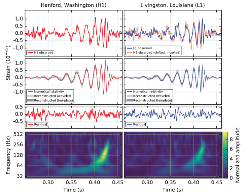
Figure 1: Summary of LIGO data (reproduced from the discovery paper).${}^{\cite[cite]{\@@bibref{Authors Phrase1YearPhrase2}{ligo}{\@@citephrase{(}}{\@@citephrase{)}}}}$ The top left panel shows the strain $h$ observed by the Hanford detector as a function of time; the top right panel shows the data for the Livingston detector with the Hanford data time-shifted, inverted and overlaid to show the excellent match between the two detectors. The data have been band pass filtered to lie in the 35-350 Hz band of maximum detector sensitivity; spectral line noise features in the detectors within this band have also been filtered. The second row shows a fit to the data using sine-Gaussian wavelets (light gray) and a different waveform reconstruction (dark gray). Also shown in color are the signals obtained from numerical relativity using the best fit parameters to the data. The third row shows for both detectors the residuals obtained by subtracting the numerical relativity curve from the filtered data in the first row. The fourth row gives a time-frequency representation of the data and shows the signal frequency increasing in time.

Binary black hole mergers take place in three stages. Initially the black holes circle their common center of mass in essentially circular orbits. During this stage they lose orbital energy in the form of gravitational radiation and spiral inward. In the second stage the black holes coalesce to form a single black hole. In the third stage, called ring-down, the merged object relaxes into its equilibrium state called a Kerr black hole.kerr Gravitational radiation is emitted copiously during merger and ring-down as well but it is the in-spiral stage that is conducive to simple analysis, and that is the basis of the back of the envelope estimates presented here. By contrast the merger and ring-down are decidedly less simple. The ring down process is not a standard component of introductory courses or textbooks on general relativity but it can be presented at that level.chandrasekhar The merger presents a formidable problem in numerical relativity that had until recently resisted all attempts at solution.numericalreview

The remainder of this paper is organized as follows. In section II we use simple arguments based on introductory physics to elucidate the underlying physics, and we use the data shown in figure 1 to estimate the masses of the black holes, their distance from earth, their initial separation and the total gravitational energy radiated. Along the way we define the chirp mass of a binary black hole system and derive the only equation that appears in the discovery paper.ligo We also present a lower bound on the total mass of the black hole pair. In our analysis we do not estimate the rotational angular momentum of the black holes either before or after the merger. In section III we discuss this and other limitations of our analysis as well as other matters of pedagogical interest. In order to make our article more useful for instructors as well as for self study we provide some problems in appendix B.

II Parameter estimation

Kepler’s third law. During the in-spiral the two black holes can be modeled as point masses of mass $M$ and $m$ that move around their common center of mass in circular orbits of radii $R$ and $r$ respectively at a common angular frequency $\omega$. The black holes remain on opposite sides of the center of mass and hence their separation is $R+r$. Obviously $Mr=mR$. At least initially, when the motion is slow and the black holes are well separated, Newtonian mechanics and Newton’s law of gravitation should apply. It is then easy to show that the frequency is related to the separation of the two black holes via

$$\omega^{2}=\frac{G(M+m)}{(R+r)^{3}},$$ (1)

which is one form of Kepler’s third law. We consider circular orbits for simplicity since our goal is only to make rough estimates. More careful analysis shows that even if the orbits were initially elliptical then emission of gravitational radiation will in any case quickly circularize the orbits.peters

Orbital energy. Continuing the Newtonian analysis of the orbiting black holes it is useful to calculate the total energy of the system, namely, the sum of the orbital kinetic energy of both black holes and their mutual gravitational potential energy.ftnt:selfenergy A short calculation reveals ftnt:energy

$$E_{{\rm tot}}=-\frac{1}{2}\frac{GMm}{(r+R)}.$$ (2)

Eq (2) gives the energy of the system as a function of the black hole separation. For later use it is convenient to use eq (1) to express the energy as a function of the frequency of the orbit instead.

$$E_{{\rm tot}}=-\frac{1}{2}\frac{G^{2/3}Mm}{(M+m)^{1/3}}\omega^{2/3}.$$ (3)

Moment of inertia. Another useful preliminary result is to calculate the moment of inertia of the orbiting black holes about their common center of mass, and to express the result in terms of the masses of the black holes and their separation $(R+r)$. The result is

$${\cal I}=\frac{mM}{m+M}(r+R)^{2}.$$ (4)

Note that as the distance between the black holes changes, the moment of inertia changes too, so it is not constant in time.

Gravitational radiation emission. Within the Newtonian framework there is no gravitational radiation and the circular orbit analyzed above should persist forever. However in general relativity the orbiting black holes will emit gravitational radiation thereby losing energy and spiraling towards each other. In order to analyze this process we need to develop a formula for the rate of gravitational radiation emission. Gravitational radiation is produced by the motion of large massive objects much as electromagnetic radiation is produced by the accelerated motion of charged particles. Under suitable conditions the electromagnetic radiation is determined by the changing electric dipole moment of the charge distribution. Similarly under suitable conditions the gravitational radiation is produced by the changing quadrupole moment of the mass distribution; the quadrupole moment is essentially the same things as the moment of inertia which is familiar from introductory physics.ftnt:dipolerad By analogy to electromagnetic dipole radiation we expect that the gravitational radiation field should be proportional to the quadrupole moment that sources it and hence the radiated power $P_{{\rm rad}}\propto{\cal I}^{2}$. This is becasue the energy density in a gravitational wave depends on the square of the field much as the energy density in an electromagnetic wave depends on the squares of the electric and magnetic fields. We also expect the radiated power to depend on the frequency $\omega$ at which the radiating system is oscillating and on the fundamental constants $G$ and $c$. Hence on dimensional grounds we expect

$$P_{{\rm rad}}=\alpha{\cal I}^{2}\omega^{\xi}G^{\eta}c^{\zeta}.$$ (5)

Here $\alpha$ is a dimensionless numerical factor and $\xi$, $\eta$ and $\zeta$ are exponents that can be determined by dimensional analysis. It is easy to verify that

$$P_{{\rm rad}}=\alpha\frac{G{\cal I}^{2}\omega^{6}}{c^{5}}.$$ (6)

The constant $\alpha$ cannot be as simply determined. A full analysis based on general relativity is needed and reveals that $\alpha=32/5$. weinberg Finally we note that to the extent that the quadrupole approximation itself is valid one can show that the angular frequency of the radiation emitted is $2\omega$. The reason for the factor of two is explained in appendix A where a more rigorous version of eq (6) is also provided. Appendix A requires some familiarity with the moment of inertia tensor which is not a standard component of an introductory physics course; however the appendix is outside the main line of development of this article and can be safely skipped. feynmanvol2

Energy Balance. Making use of eqs (6) and (4) and (1) we see the power of gravitational radiation emission by the binary black holes is given by

$$P_{{\rm binary}}=\alpha\frac{G^{7/3}\omega^{10/3}}{c^{5}}\frac{m^{2}M^{2}}{(m+M)^{2/3}}$$ (7)

On the other hand the rate at which the binary black holes lose orbital energy is obtained by differentiating eq (3)

$$-\frac{dE_{{\rm tot}}}{dt}=\frac{1}{3}G^{2/3}\frac{Mm}{(M+m)^{1/3}}\omega^{-1/3}\frac{d\omega}{dt}.$$ (8)

Equating the energy loss (8) to the power radiated (7) yields

$$\frac{(mM)^{3/5}}{(m+M)^{1/5}}=\frac{c^{3}}{G}\left(\frac{1}{3\alpha}\omega^{-11/3}\frac{d\omega}{dt}\right)^{3/5}.$$ (9)

It is conventional to define the chirp mass ${\cal M}$ as the left hand side of eq (9). The chirp mass is a crucial scale in the in-spiral process.

The Chirp. In order to compare to the data it is helpful to rewrite eq (9) in terms of $f$ the frequency of observed radiation. Equating $2\pi f$ to $2\omega$ (keeping in mind that the frequency of radiation is twice that of the orbital frequency), we have that $\omega=\pi f$. Making this substitution in eq (9) we obtain

$${\cal M}=\frac{c^{3}}{G}\left(\frac{1}{3\alpha}\pi^{-8/3}f^{-11/3}\frac{df}{dt}\right)^{3/5}.$$ (10)

Setting $\alpha=32/5$ Eq (10) precisely matches the only equation in the LIGO discovery paper. ligo Eq (10) shows that as the black holes spiral inward the frequency of the emitted radiation increases rapidly. This is the famous chirp. To make this more explicit we can integrate eq (10) to show that ftnt:chirp

$$\frac{1}{f_{1}^{8/3}}-\frac{1}{f_{2}^{8/3}}=8\alpha\pi^{8/3}\frac{G^{5/3}{\cal M}^{5/3}}{c^{5}}\tau.$$ (11)

Here $f_{1}$ is the initial frequency and $f_{2}$ is the frequency after a time $\tau$. Eq (11) shows that the frequency rises rapidly from the value $f_{1}$ and diverges in a finite amount of time $\tau_{\infty}$. Of course the divergence is spurious and the rise in frequency is eventually interrupted by the coalescence of the black holes as we will see below.

Estimating the chirp mass. The bottom panel in fig 1 shows the variation of the frequency of the observed gravitational radiation as a function of time. The frequency indeed rises rapidly as predicted by eq (11). Assuming $f_{2}\gg f_{1}$ we may neglect the second term on the right hand side of eq (11) to obtain

$${\cal M}=\frac{c^{3}}{Gf_{1}}\frac{1}{(8\alpha f_{1}\tau)^{3/5}\pi^{8/5}}$$ (12)

Inspection of the bottom left panel of figure 1 shows that $f_{1}\approx 42$ Hz at time 0.35 s and that the frequency essentially diverges at time 0.43 s. Hence $\tau\approx 0.08$ s. Substituting these values of $f_{1}$ and $\tau$ in eq (12) yields ${\cal M}=35$ solar masses, very close to the value of 30 solar masses obtained by the LIGO collaboration. In keeping with the spirit of a back of the envelope estimate we do not attempt to estimate the uncertainty in our result. However if we pick other reasonable values of $f_{1}$ and $\tau$ from the data we always find values of ${\cal M}$ close to 30 $M_{{\odot}}$.

Bound on the total mass. The chirp mass gives an idea of the scale of the system but it does not by itself reveal the individual masses of the two black holes. If the two black hole masses are equal then it follows from the definition of the chirp mass that the total mass of the pair is $(4)^{3/5}{\cal M}$. For ${\cal M}=30M_{{\odot}}$ this amounts to a total mass of $70M_{{\odot}}$ or $35M_{{\odot}}$ per black hole. More generally one can show that if the chirp mass is ${\cal M}$ then the total mass of the pair has to be greater than $(4)^{3/5}{\cal M}$. To show this assume that the $m=\xi M_{{\rm tot}}$ and $M=(1-\xi)M_{{\rm tot}}$. Here the fraction $\xi$ lies in the range $0<\xi<1$. From the definition of the chirp mass it follows

$$M_{{\rm tot}}=\frac{{\cal M}}{[\xi(1-\xi)]^{3/5}}.$$ (13)

Over the unit interval the quantity $\xi(1-\xi)$ is maximum at $\xi=1/2$ which rigorously justifies the lower bound on $M_{{\rm tot}}$ noted above.

Schwarzschild radius; Event horizon. It is a standard exercise in introductory physics to show that at a distance $r$ from the center of a spherical body of mass $M$ the escape velocity is $\sqrt{2GM/r}$ (assuming that $r$ is greater than the radius of the spherical body). Setting the escape velocity equal to the speed of light $c$ we obtain the Schwarzschild radius $R_{s}$ of the body given by

$$R_{s}=\frac{2GM}{c^{2}}.$$ (14)

If the spherical body is sufficiently dense that it is smaller than $R_{s}$ then it has an event horizon and is a black hole. The event horizon is a sphere of radius $R_{s}$ that surrounds the black hole. Particles that travel slower than the speed of light can escape the black hole only if they remain outside the event horizon. Although our analysis is based on Newtonian gravity the same conclusion emerges from classical general relativity: only particles that remain outside the event horizon can escape the black hole and the radius of the event horizon is given by eq (14). Furthermore in classical general relativity a particle that is inside the event horizon can never emerge outside, a restriction not present in Newtonian gravity. weinberg

Merger and chirp cutoff. The black holes will begin to coalesce once their separation is equal to the sum of their Schwarzschild radii. In other words

$$R+r=\frac{2G}{c^{2}}(M+m).$$ (15)

At this separation according to eq (1) the angular frequency of the orbiting black holes is

$$\omega_{c}=\frac{1}{\sqrt{8}}\frac{c^{3}}{G(M+m)}.$$ (16)

Hence we estimate that the highest frequency attained by the chirp is $f_{c}=\omega_{c}/\pi$.

Estimating the black hole masses. It follows from eq (16) that

$$M_{{\rm tot}}=M+m=\frac{1}{\pi\sqrt{8}}\frac{c^{3}}{Gf_{c}}.$$ (17)

Inspection of the bottom left panel of figure 1 suggests the value $f_{c}=300$ Hz which yields $M_{{\rm tot}}=76M_{{\odot}}$ , in remarkable agreement with $M_{{\rm tot}}=65M_{{\odot}}$ obtained by the LIGO collaboration. In order to determine the individual masses of the black holes we use ${\cal M}=30M_{{\odot}}$ and $M_{{\rm tot}}=76M_{{\odot}}$. Eq (13) then yields $\xi=0.7$ implying that the individual black hole masses are 53 and 23 solar masses respectively (in fair agreement with the values of 36 and 29 solar masses obtained by the LIGO collaboration).

Estimating the total energy radiated. Perhaps the most awe-inspiring fact about GW150914 is the staggering amount of energy emitted in the form of gravitational radiation. The LIGO collaboration determined that the energy equivalent of 3 solar masses was emitted in just a tenth of a second. Making use of Einstein’s formula $E=mc^{2}$ that is approximately $5\times 10^{47}$ J. By way of comparison the sun emits $4\times 10^{25}$ J in the form of electromagnetic radiation in a tenth of a second; over its entire lifespan of several billion years the sun will radiate less than one percent of its mass. We can estimate the total gravitational energy radiated by using eq (2) for the energy of the orbiting black holes. ftnt:energycaveat For the purpose of this estimate we assume that the final separation of the black holes is the sum of their Schwarzschild radii and that the initial separation is much larger and may be taken to be essentially infinite. Substituting eq (15) in eq (2) yields

$$\frac{1}{4}\left(\frac{Mm}{M+m}\right)c^{2}$$ (18)

as the estimate of the total amount of gravitational wave energy radiated. Setting $M=36M_{\odot}$ and $m=29M_{\odot}$ yields 4$M_{\odot}$ as the estimated energy radiated in good agreement with the value of 3$M_{\odot}$ determined by LIGO. Eq (18) also reveals that for a fixed total mass $M+m$, the radiated energy is maximized when the  merging black hole masses are equal and diminishes greatly if one of the merging objects is much lighter than the other.

Estimating the initial separation. Another quantity we can estimate once the total mass of the two black holes is known is the separation of the black holes when the gravitational radiation first becomes detectable. From the bottom left panel of figure 1 we see that the frequency of gravitational radiation is approximately 45 Hz when the in-spiral process first becomes observable. Substituting this frequency in eq (1) and taking the total mass of the two black holes to be 65 $M_{\odot}$ reveals that the initial separation of the black holes was about 800 km. The combined Schwarzschild radii of the two black holes on the other hand are approximately 100 km.

Gravitational wave amplitude. Gravitational waves alternately stretch and compress the space through which they propagate. The amplitude of a gravitational wave denoted $h$ is the fractional amount by which the wave stretches or compresses space or the distance between the two ends of an interferometer arm; $h$ is a dimensionless quantity. Assuming that the intensity of a gravitational wave is proportional to the square of the amplitude, it is a simple exercise in dimensional analysis to show that the intensity is given by

$${\cal I}_{{\rm rad}}=\beta h^{2}\frac{f^{2}c^{3}}{G}.$$ (19)

The intensity is the energy flow per unit time per unit area normal to the direction of propagation and $\beta$ is a dimensionless constant of order unity. A full analysis based on linearized general relativity shows that $\beta=\pi/2$. weinberg

Estimating the distance. The intensity of gravitational radiation at a distance $R$ from in-spiraling binary black holes is directional but on average falls off with distance as ${\cal I}_{{\rm rad}}=P_{{\rm rad}}/4\pi R^{2}$. Using this inverse square law, eq (7) and eq (19) we can then determine $R$ in terms of the observed $h$ and $f$ as

$$R=\frac{4}{\sqrt{5}}\pi^{2/3}\frac{G^{5/3}}{c^{4}}\frac{1}{h}f^{2/3}\frac{mM}{(m+M)^{1/3}}.$$ (20)

From the second panel on the left of figure 1 we see that $h\approx 10^{-21}$ for $f\approx 250$ Hz. Using these values and $m=29$ and $M=36$ solar masses we determine the distance of the GW150914 to be 1.7 billion light years in good agreement with the 1.3 billion light years determined by LIGO. The agreement is surprisingly good since the same caveats apply to eq (20) as to eq (18) and in addition we have ignored the directionality of quadrupole radiation.

Directional information. With just two detectors in operation it was not possible to pinpoint the exact direction of the source. The signal arrived at the Louisiana detector before the one in Washington by 7 milliseconds. Given the approximate latitude and longitude of the detectors one can deduce that the distance between the detectors is 3000 km or 10 ms at the speed of light. If the direction of propagation of the gravitational waves was parallel to the displacement between the two sites the delay would be exactly 10 ms. On the other hand if the direction of propagation was perpendicular to the displacement vector the signal would arrive simultaneously at the two detectors. The delay of 7 ms implies that the direction of propagation makes an angle of 45^∘ with the displacement vector (see problem). GW150914 therefore lies on a circle on the sky that subtends an angle of 45^∘. This is as far as one can go with a single delay time but the LIGO collaboration used the entire time dependence of both signals to further pinpoint particular arcs along this circle that are more likely to have been the location of the source (see figure 4 of ref ligoprops, ). Directional information is important because it allows study of the same source by other more traditional channels such as gamma ray and neutrino astronomy. In the future it is expected that the two LIGO detectors at Livingston and Hanford will be joined by a third detector that will allow more precise location of future sources.

III Discussion

The above Newtonian analysis gives surprisingly good agreement with the parameters obtained by the fully relativistic treatment used by LIGO. In addition to the numerous simplifications explicitly stated above, we also ignore polarization of the gravitational radiation and the spin of the black holes. Incorporation of these effects and other refinements is certainly possible but is contrary to the spirit of the ballpark estimates that we wished to present. Because of the approximations made our estimates should be correct only to order of magnitude (although serendipitously in many instances our estimates are within a factor of two of the best fit obtained by LIGO).

Prior to LIGO the best evidence for gravitational waves came from observations of binary pulsars.taylornobel ; taylor Whereas LIGO is able to detect the actual distortion of space caused by the passage of gravitational waves, binary pulsars only provide indirect evidence for gravitational waves. Furthermore it is estimated that the best studied Hulse-Taylor binary pulsar will take 300 million years to coalesce (see problem 8 in appendix B). Thus for the foreseeable future the binary pulsar provides access only to the in-spiral phase whereas LIGO’s binary black hole has provided a view of the strong gravity physics of coalescence and ring-down.

Finally we briefly discuss physics after the merger. During the ring-down phase the signal from the merged black hole resembles the transients of a under-damped harmonic oscillator familiar from introductory physics (see figure 1). This transient corresponds to the longest lived “quasi-normal” mode of the black hole space-time. The damping rate and ringing frequency of the quasi-normal mode are determined by the mass and spin of the quiescent black hole that forms after the quasi-normal modes have died away. Thus the spins of the initial black holes can be determined using the in-spiral data and the spin of the final merged object using the ring-down data. By verifying that the initial and final spins are consistent with each other using a numerical analysis of the merger the LIGO team were able for the first time to test General Relativity in the hitherto inaccessible strong field regime, another significant outcome of their discovery.viewpoints ; ligogr

Note added. After completion of this work we learnt of a new e-print from the LIGO-VIRGO collaboration that covers some of the same ground as the present manuscript.ligoped We thank Andrew Matas, Laleh Sadeghian and Madeleine Wade for bringing ref ligoped to our attention and Ofek Birnholtz and Alex Nielsen for a helpful correspondence.

Appendix A Quadrupole Tensor

The purpose of this section is to introduce the quadrupole tensor by analogy to the moment of inertia tensor. This section thus requires some familiarity with the moment of inertia tensor, which is not typically included in an introductory physics course but is accessible at the level of feynmanvol2 . Consider a system of $n$ particles with mass $m_{i}$ and position $(x_{i},y_{i},z_{i})$ with $i=1,2,3,\ldots,n$. The moment of inertia tensor has components

$$I_{xx}=\sum_{i=1}^{n}m_{i}(y_{i}^{2}+z_{i}^{2});\hskip 5.69054ptI_{xy}=-\sum_{i=1}^{n}m_{i}x_{i}y_{i};$$ (21)

and the form of the other diagonal and off-diagonal components can be written down by analogy.feynmanvol2 The quadrupole tensor is very similar. The off-diagonal components differ only in sign, e.g., $Q_{xy}=-I_{xy}$. The diagonal components have the form $Q_{xx}=-I_{xx}+\frac{1}{3}\overline{I}$ and similarly for $Q_{yy}$ and $Q_{zz}$. Here $\overline{I}=I_{xx}+I_{yy}+I_{zz}$. In terms of the quadrupole tensor the power of gravitational radiation emitted is given by

$$P_{{\rm rad}}=\frac{1}{5}\frac{G}{c^{5}}\sum_{\alpha,\beta=x,y,z}\left(\frac{d^{3}Q_{\alpha\beta}}{dt^{3}}\right)^{2}.$$ (22)

Now suppose for simplicity that the rotating system lies in the $x$-$y$ plane and rotates about the $z$-axis. After a half rotation the components of the the quadrupole tensor will have returned to their original values. As far as the quadrupole moment goes the radiating system is back to its original state after just half a rotation; hence the frequency of the radiation is twice the frequency of rotation.

Appendix B Problems

Problems 1, 2 and 3 provide additional information about the LIGO discovery; problem 4 is on a different application of the two body circular orbit discussed in Section II: and problems 5, 6 and 7 treat electromagnetic radiation and radiation reaction effects that are analogous to the gravitational effects analyzed in the main body of the paper. Problem 8 analyzes the gravitational radiation due to the in-spiral of the Hulse-Taylor binary pulsar. The problems vary in level of difficulty.

Problem 1. What’s in a name? (a) The discovery event is designated GW150914. Explain why. Hint: Re-read the first paragraph of the Introduction. (b) The second black hole merger event observed by LIGO was designated GW151226. ligo2 What can you deduce from the name of the event?

Problem 2. Sensitivity of LIGO. The length of an arm of LIGO’s interferometer is 4 km. By how much is this distance changed due to a gravitational wave with amplitude $h=10^{-21}$? Give your answer in m. Compare to the radius of a proton (approximately 0.9$\times 10^{-15}$ m).

Problem 3. Delay and direction. (a) Using the latitude and longitude information for the two detectors verify that the distance between the two detectors is 3000 km. (b) Suppose that the direction of propagation makes an angle $\theta$ with the displacement from the Livingston detector to the Hanford detector. Show that delay in the arrival at Hanford is given by $d\cos\theta/c$ where $d$ is the distance between the two detectors.

Problem 4. Discovery of the first extra solar planet. A star of mass $M$ and a planet of mass $m$ orbit their center of mass in circular orbits of radius $R$ and $r$ respectively at a common frequency $\omega$. The orbits are in the $x$-$y$ plane and the center of mass is at the origin. The earth lies on the negative $y$-axis many light years distant. The planet cannot be seen from Earth but the $y$-component of the velocity of the star can be measured spectroscopically and will evidently oscillate at the frequency $\omega$ with an amplitude $R\omega$. For the star 51 Pegasus the velocity was observed to oscillate with a period of 4.23 days and an amplitude of 60 m/s leading to the discovery the first extra solar planet, 51 Pegasi B.c51peg Spectroscopically the star resembles the sun and hence it is reasonable to assume $M=M_{{\odot}}=2.0\times 10^{30}$ kg. (a) Use eq (1) and the measured period to determine $R+r$ the distance between the star and planet. You may neglect the mass of the planet. Give your answer in astronomical units. (1 A.U. = 1.5 $\times 10^{11}$ m). (b) Use the measured amplitude and period to determine $R$. Then combine with your result of part (a) to determine $m$, the mass of the planet. Compare to the mass of Jupiter (2 $\times 10^{27}$ kg).

Answer to Problem 4. (a) 0.05 A.U. (b) $R=3.5\times 10^{6}$ m. $m=0.9\times 10^{27}$ kg.

Problem 5. Electromagnetic dipole radiation. (a) Dimensional analysis. In the S.I. system it is most convenient to express the units of all quantities in terms of kg, m, s and C. For example Coulomb’s law reveals that the units of $\epsilon_{0}$ are C² s²/kg m³. Determine the units of the electric dipole moment and the magnetic dipole moment.
(b) Electric dipole radiation. A rotating electric dipole moment will produce radiation. Determine the dependence of the power radiated $P_{{\rm electric}}$ on the magnitude of the dipole moment, $p$, the angular frequency of rotation, $\omega$, and the basic electromagnetic constants $\epsilon_{0}$ and $c$ using dimensional analysis. (c) Magnetic dipole radiation. Determine the dependence of the power radiated by an rotating magnetic dipole, $P_{{\rm mag}}$, on the magnitude of the dipole moment, $d$, the angular frequency of rotation, $\omega$, and the electromagnetic constants $\epsilon_{0}$ and $c$ using dimensional analysis.

Answer 5. (a) Electric dipole moment: C m. Magnetic dipole moment: C m²/s. (b) $P_{{\rm electric}}=(1/6\pi)(\omega^{4}p^{2}/\epsilon_{0}c^{3})$. This result is called Larmor’s formula. (c) $P_{{\rm mag}}=(1/6\pi\epsilon_{0})(\omega^{4}d^{2}/\epsilon_{0}c^{5})$. In both (b) and (c) the pre-factor of $1/6\pi$ cannot be determined by dimensional analysis; a full derivation based on Maxwell’s equations is necessary.

Problem 6. Spin down of the Crab Nebula Pulsar. (a) Model the pulsar as a sphere with moment of inertia $I$ and a magnetic dipole $d$ that rotates at an angular frequency $\omega$. Assuming that the dominant mechanism for the pulsar to lose rotational kinetic energy is via magnetic dipole radiation show that the pulsar slows down according to the equation $d\omega/dt=-\omega^{3}\tau$ where the time scale $\tau=d^{2}/\epsilon_{0}Ic^{5}$. (b) Integrate the result of part (a) to show that $\omega^{-2}-\omega_{0}^{-2}=2t\tau$ where $\omega_{0}$ is the angular frequency of the pulsar at time $t=0$ when it was initially created, $\omega$ is the angular frequency at time $t$. Assuming that $\omega_{0}\gg\omega$ it follows that the age of the pulsar is $t\approx 1/2\omega^{2}\tau$. (c) The Crab Nebular pulsar was discovered in the 1960s. At that time astronomers measured $\omega=200$ s${}^{-}1$ and $d\omega/dt=2.6\times 10^{-9}$ s^-2. Use these data to determine $\tau$ and the age in years of the Crab Nebular pulsar. The pulsar is believed to have been born from the supernova recorded by Chinese astronomers in the year 1054. ostriker

Problem 7. Classical lifetime of Bohr atom. According to the Bohr model the electron orbits an essentially stationary proton in an orbit of radius $a_{B}=0.53{\rm\AA}$. Show that according to classical electromagnetism the electron should spiral inward and merge with the proton in a time $\tau=(1/4)(4\pi\epsilon_{0}m/e^{2})^{2}c^{3}a_{B}^{3}$ where $m$ is the mass of an electron. Determine $\tau$ in seconds. For simplicity you may use non-relativistic mechanics throughout.

Hint for Problem 7. Calculate the total kinetic and potential energy for a circular orbit of radius $r$. Note that as the electron orbits the electric dipole moment of the atom rotates leading to electric dipole radiation. Use the result of problem 5(b) and energy conservation to show that the electron spirals inward.

Problem 8. Gravitational radiation from binary pulsar. The Hulse-Taylor binary pulsar consists of two neutron stars, one a pulsar.taylornobel By timing the pulsar it has been discovered that the orbital period is 7.75 hours and the two stars have a mass of approximately 1.4 $M_{{\odot}}$ each. (a) Assuming a circular orbit use eq (9) to estimate how much the period decreases per year. (b) Use eq (11) to estimate the time for the binary pulsar to coalesce.

Answer 8. (a) 10 $\mu$s. (b) 1 billion years. Discussion: The orbit is actually highly elongated with an eccentricity of 0.62. Because of the regularity of the pulses and the exquisite precision with which their times are measured the masses of the neutron stars are actually known to five significant figures and the eccentricity to seven. Taking the eccentricity into account peters it is found that the period actually decreases 76.5 $\mu$s per year which agrees with the observed value to within one percent.taylor The time to coalesce is 300 million years when eccentricity is taken into account.

Figure 1
Summary of LIGO data (reproduced from the discovery paper). ligo The top left panel shows the strain $h$ observed by the Hanford detector as a function of time; the top right panel shows the data for the Livingston detector with the Hanford data time-shifted, inverted and overlaid to show the excellent match between the two detectors. The data have been band pass filtered to lie in the 35-350 Hz band of maximum detector sensitivity; spectral line noise features in the detectors within this band have also been filtered. The second row shows a fit to the data using sine-Gaussian wavelets (light gray) and a different waveform reconstruction (dark gray). Also shown in color are the signals obtained from numerical relativity using the best fit parameters to the data. The third row shows for both detectors the residuals obtained by subtracting the numerical relativity curve from the filtered data in the first row. The fourth row gives a time-frequency representation of the data and shows the signal frequency increasing in time.

References

- (1) B.P. Abbott et al., Observation of Gravitational Waves from a Binary Black Hole Merger, Physical Review Letters 116, 061102-061118 (2016); https://doi.org/10.1103/PhysRevLett.116.061102
- (2) See for example, E. Berti, The First Sounds of Merging Black Holes, Physics 9, 17 (2016); F. Pretorius, Relativity Gets Thorough Vetting from LIGO, Physics 9, 52 (2016); M. Buchanan, Backrgound Noise of Gravitational Waves. Physics 9, 33 (2016).
- (3) Kerr black holes rotate; Schwarzschild black holes are non-rotating. For an authoritative popular introduction to black holes see K. Thorne, The Science of Interstellar (W.W. Norton, 2014).
- (4) S. Chandrasekhar, Mathematical Theory of Black Holes (Oxford, 1983) has an authoritative introduction.
- (5) For an introduction see, for example, T.W. Baumgarte and S.L. Shapiro, Numerical Relativity (Cambridge, 2010).
- (6) P.C. Peters, Gravitational Radiation and the Motion of Two Point Masses, Physical Review 136, B1224-B1232 (1964).
- (7) S. Weinberg, Gravitation and Cosmology (John Wiley, 1972).
- (8) For a notable exception see chapter 31 of R.P. Feynman, R.B. Leighton and M. Sands, The Feynman Lectures on Physics, vol 2 (Addison-Wesley, 1964).
- (9) B.P. Abbott et al., Properties of the Binary Black Hole Merger GW150914, Physical Review Letters 116, 241102-241121 (2016).
- (10) For an overview see the Nobel Prize lectures by R.A. Hulse, The discovery of the binary pulsar, Reviews of Modern Physics 66, 699-710 (1994), and J.H. Taylor, Binary pulsars and relativistic gravity, Reviews of Modern Physics, 66, 711-719 (1994).
- (11) J.M. Weisberg, D.J. Nice and J.H. Taylor, Timing Measurements of the Relativistic Binary Pulsar PSR B1913+16, Astrophysical Journal 722, 1030-1034 (2010).
- (12) B.P. Abbott et al. Tests of general relativity with GW150914, Physical Review Letters 116, 221101-221120 (2016).
- (13) B.P. Abbott et al., GW151226: Observation of Gravitational Waves from a 22-Solar-Mass Binary Black Hole Coalescence, Physical Review Letters 116, 241103-241117 (2016).
- (14) M. Mayor and D. Queloz, A Jupiter-mass companion to a solar-type star, Nature 378, 355-360 (1995).
- (15) J.P. Ostriker and J.E. Gunn, On the Nature of Pulsars, Astrophysical Journal 157, 1395-1417 (1969).
- (16) B.P. Abbott et al., The basic physics of the binary black hole merger GW150914, Annalen Der Physik 529, 1600209 (2017).
- (17) For the duration of the in-spiral it is acceptable to treat the black holes as particles of fixed mass and the only relevant gravitational potential energy is the mutual potential energy of the two black holes, not their individual self-energy.
- (18) The reader will notice that the total energy is one half the potential energy. This is an example of the virial theorem in classical mechanics, but students of introductory physics can derive the result by adding up all the contributions to the orbital energy. The potential energy is obviously . The kinetic energy is given by . Making use of eq (1) for and eq (4) for the moment of inertia leads quickly to the result quoted in eq (2) for the total energy.
- (19) By way of comparison, electromagnetic radiation is predominantly produced by the changing electric or magnetic dipole moments. The quadrupole component matters only if the dipole moments of the radiating system vanish by symmetry. See problem 5 in appendix B for more on electromagnetic dipole radiation.
- (20) To obtain eq (11) first write eq (10) in the form and integrate both sides. Take the lower limit on the time integral and the upper limit as . The corresponding limits on the integral are and respectively, yielding eq (11).
- (21) By so doing we are approximating the total energy radiated by the energy radiated during the in-spiral process alone. Although the peak power is radiated during the merger, inspection of fig 1 suggests that the power radiated during in-spiral is indeed comparable to the total power radiated during the entire process, thereby justifying the estimate in eq (18).