Joanna Slawinska\correspondingauthorJoanna Slawinska, Center for Environmental Prediction, Rutgers, The State University of New Jersey, 14 College Farm Road, New Brunswick, NJ, 08901
\extraaffilCenter for Environmental Prediction, Rutgers, The State University of New Jersey,
New Brunswick, New Jersey, USA
Indo-Pacific variability on seasonal to multidecadal timescales.
Part II: Multiscale atmosphere-ocean linkages
Abstract
The coupled atmosphere-ocean variability of the Indo-Pacific on interannual to multidecadal timescales is investigated in a millennial control run of CCSM4 and in observations using a family of modes recovered in Part I of this work from unprocessed SST data through nonlinear Laplacian spectral analysis (NLSA). It is found that ENSO and combination modes of ENSO with the annual cycle exhibit a seasonally synchronized southward shift of equatorial surface zonal winds and thermocline adjustment consistent with terminating El Niño and La Niña events. The surface wind patterns associated with these modes also generate teleconnections between the Pacific and Indian Oceans, leading to a pattern of SST anomalies characteristic of the Indian Ocean dipole. Fundamental and combination modes representing the tropospheric biennial oscillation (TBO) in CCSM4 are also found to be consistent with mechanisms for seasonally synchronized biennial variability of the Asian-Australian monsoon and Walker circulation. On longer timescales, the leading multidecadal pattern recovered by NLSA from Indo-Pacific SST data in CCSM4, referred to as west Pacific multidecadal mode (WPMM), is found to significantly modulate ENSO and TBO activity with periods of negative SST anomalies in the western tropical Pacific favoring stronger ENSO and TBO variability. Physically, this behavior is attributed to the fact that cold WPMM phases feature anomalous decadal westerlies in the tropical central Pacific and easterlies in the tropical Indian Ocean, as well as an anomalously deep thermocline in the eastern Pacific cold tongue. Moreover, despite the relatively low SST variance explained by this mode, the WPMM is found to correlate significantly with decadal precipitation over Australia in CCSM4.
1 Introduction
The Indo-Pacific is the arena of prominent modes of coupled atmosphere-ocean variability spanning seasonal to multidecadal timescales. Notably, it is the region where the El Niño-Southern Oscillation (ENSO), the dominant mode of interannual climate variability (Bjerknes 1969; Philander 1990; Neelin et al. 1998; Wang and Picaut 2004; Sarachik and Cane 2010; Trenberth 2013), takes place. ENSO is well known to exhibit a phase synchronization with the seasonal cycle (Rasmusson and Carpenter 1982), with El Niño and La Niña events typically developing in the boreal summer, peaking during the following winter, and dissipating in the ensuing spring. This phase synchronization has been explained through quadratic nonlinearities in the coupled atmosphere-ocean system producing a cascade of frequencies known as ENSO tones, whose associated temporal and spatial patterns are called ENSO combination modes (Stein et al. 2011, 2014; McGregor et al. 2012; Stuecker et al. 2013, 2015a; Ren et al. 2016). In particular, the ENSO combination modes at the sum and difference of the dominant ENSO frequency and the annual cycle frequency project strongly on the surface atmospheric circulation and thermocline depth and are believed to play an important role in restoring El Niño/La Niña conditions to neutral conditions. A prominent feature of ENSO caused by nonlinear dynamics is an asymmetry between El Niño and La Niña phases, which is manifested in positively skewed SST anomaly distributions (Burgers and Stephenson 1999; An and Jin 2004; Weller and Cai 2013).
In addition to ENSO and ENSO combination modes, other modes of interannual Indo-Pacific climate variability which have received significant attention are the Indian Ocean dipole (IOD; Saji et al. 1999; Webster et al. 1999) and the tropospheric biennial oscillation (TBO; Meehl 1987, 1993, 1994, 1997; Li and Zhang 2002; Li et al. 2006). The IOD is characterized by SST anomalies of opposite sign developing in the eastern and western Indian Ocean, whereas the TBO is generally associated with biennial variability of the Asian-Australian monsoon (Li 2013). Similarly to ENSO, the IOD and TBO exhibit a seasonally locked behavior. The existence and significance of linkages between ENSO and these phenomena are areas of active research (Goswami 1995; Annamalai et al. 2003; Li et al. 2006; Zhao and Nigam 2015).
The Indo-Pacific is also the arena of prominent modes of decadal variability, the most known of which are the Pacific Decadal oscillation (PDO; Mantua et al. 1997) and the Interdecadal Pacific Oscillation (IPO; Power et al. 1999). These two modes are generally thought to be a manifestation of the same phenomenon, and differ mainly in their domain of definition (the PDO is defined over the North Pacific, whereas the IPO is defined over the whole Pacific basin). The physical nature of these modes, and more broadly Pacific decadal variability, has been investigated intensively over the last 20 years, and while a number of hypotheses have emerged, consensus on the validity of these hypotheses is limited. Some studies find that the dominant decadal modes retrieved using classical methods such as empirical orthogonal function (EOF) analysis are merely residuals of ENSO after low-pass filtering; in particular, residuals due to El Niño/La Niña asymmetries resulting from nonlinear dynamics (Rodgers et al. 2004; Vimont 2005; Sun and Yu 2009; Watanabe and Wittenberg 2012; Sun et al. 2014; Wittenberg et al. 2014). For instance, Vimont (2005) constructs a decadal ENSO-like signal through a linear combination of three interannual modes, with no decadal mode involved, and shows that a low-frequency spatiotemporal residual results from the different spatiotemporal characteristics of these three modes, which can be associated in turn with the ENSO precursor, peak, and “leftover”. Moreover, Rodgers et al. (2004) find that the dominant decadal patterns of SST and thermocline depth, extracted via EOF analysis of low-pass filtered, meridionally averaged, Z20 data over the equatorial Pacific, bear strong similarities to composite patterns representing El Niño/La Niña asymmetries. In light of this finding, they argue that the dominant patterns recovered from decadal low-pass filtered data are a consequence (rather than a cause) of ENSO asymmetries.
At the same time, other studies associate Pacific decadal variability with an intrinsic physical signal due to one or more stochastic processes (Cane et al. 1995; Thompson and Battisti 2001; Okumura 2013), tropical/ENSO-like dynamics (Knutson and Manabe 1998; Yukimoto et al. 2000; Liu et al. 2002), or remote forcing from the mid-latitudes (Kirtman and Schopf 1998; Barnett et al. 1999; Kleeman et al. 1999; Gu and Philander 1997; Pierce et al. 2000; Vimont et al. 2001, 2003; Solomon et al. 2003). Frequently, decadal and multidecadal fluctuations are not associated with a single physical mode, but are considered as multiple phenomena acting simultaneously (Deser et al. 2010; Newman et al. 2015), or they are viewed as changes in the mean background state (Wang and Ropelewski 1995). Such changes may be produced by quasi-decadal variability (Hasegawa and Hanawa 2006), global warming (Timmermann et al. 1999), the last glacial maximum (An et al. 2004), or climate shifts (e.g., Ye and Hsieh 2006) that are, most often, attributed to the IPO (Salinger et al. 2001; Imada and Kimoto 2009). Decadal modulations of the tropical biennial oscillation (TBO) have also been studied (e.g., Meehl and Arblaster 2011, 2012), though less extensively than ENSO. Arguably, progress in elucidating the relation between decadal and interannual variability is hampered by the fact that the extraction of decadal modes through conventional data analysis techniques such EOF analysis often requires ad hoc preprocessing of the data (e.g., low-pass filtering), compounding the physical interpretation of the results.
Irrespective of its origins and nature, the impacts of the Indo-Pacific multidecadal variability have been documented in numerous studies. Power et al. (1999) find that ENSO’s impact on Australian precipitation depends strongly on the IPO phase, and Silva et al. (2011) report an IPO modulation of ENSO’s impact on South American precipitation. Dai (2013) has found a strong correlation of the IPO with anomalously dry and wet decades occurring over the western and central United States in the 20th century. Moreover, multidecadal droughts in the Indian subcontinent and the southwestern United States have also been attributed to the IPO (Meehl and Hu 2006), and the rapid sea level rise/fall observed over the last 17 years over the western/eastern tropical Pacific (called east–west dipole by Meyssignac et al. 2012) has been associated with the PDO (e.g., Zhang and Church 2012). Meehl et al. (2013), England et al. (2015), and others have associated the decades of global warming hiatus observed during the 20th century with negative phases of the IPO.
A major challenge in research on decadal variability is the relatively short observational record from which it is difficult to robustly extract modes operating at decadal timescales and to project their activity into the future. Han et al. (2014) examined a longer observational record and showed that the IPO does not explain in itself sea level rise over certain decades. Based on this finding, they hypothesized the existence of another decadal mode. They argued that this mode acts mainly over the tropical Indian Ocean (as opposed to the IPO which is active in the Pacific Ocean), but did not address the question of its origin. England et al. (2014) analyzed the most recent hiatus and associated it with exceptionally strong trade winds (also considered responsible for sea-level rise by Han et al. (2014)) and increased heat uptake by the ocean. Notably, they observed that the magnitude of trade-wind strengthening cannot be explained solely by the IPO, suggesting that other factors, e.g., the internal variability of the Indian Ocean, should play a role. Without further explanation of the origin of trade-wind enhancement, a heat budget analysis of the modeled hiatus was performed based on a simulation with prescribed values of trade winds (as models fail to produce as strong winds as observed; see Luo et al. (2012)).
Several other studies (Karnauskas et al. 2009; Solomon and Newman 2012; Seager et al. 2015) also stress the need to consider modes of Indo-Pacific internal variability other than the IPO to build a more complete explanation of the recent climatic record. In particular, the second EOF of SST (Timmermann 2003; Yeh and Kirtman 2004; Sun and Yu 2009; Ogata et al. 2013), the spatial pattern of which consists mainly of an equatorial SST zonal dipole, have been sometimes associated with observed decadal fluctuations. Some authors (e.g., Choi et al. 2009, 2012; Ogata et al. 2013) have argued that decadal modulations of ENSO are driven by this background state.
In Part I of this work (Slawinska and Giannakis 2016), we constructed a family of spatiotemporal modes of Indo-Pacific SST variability in models and observations using a recently developed eigendecomposition technique called nonlinear Laplacian spectral analysis (NLSA; Giannakis and Majda 2011, 2012a, 2012b, 2013, 2014; Giannakis 2015). A key feature of this method is that it can simultaneously recover modes spanning multiple timescales without pre-filtering the input data. In Part I, we used NLSA to recover a family of Indo-Pacific SST modes from a 1,300 y integration of the Community Climate System Model version 4 (CCSM4; Gent et al. 2011) and and a 800 y integration of the Geophysical Fluid Dynamics Laboratory coupled climate model CM3 (Griffies et al. 2011), as well as from monthly-averaged HadISST data (Rayner et al. 2003) for the industrial and satellite eras. This family consists of modes representing (i) the annual cycle and its harmonics, (ii) the fundamental component of ENSO and its associated combination modes with the annual cycle (denoted ENSO-A modes), (iii) the TBO and its associated TBO-A combination modes, (iv) the IPO, and (v) a west Pacific multidecadal mode (WPMM) featuring a prominent cluster of SST anomalies in the western equatorial Pacific.
Compared to modes recovered by classical EOF-based approaches, the mode family identified in Part I has minimal risk of mixing intrinsic decadal variability with residuals associated with low-pass filtered interannual modes (since NLSA operates on unprocessed data). Moreover, unlike EOF analysis which mixes distinct ENSO combination frequencies into single modes (McGregor et al. 2012; Stuecker et al. 2013), the NLSA-based ENSO-A modes resolve individual ENSO frequencies and have the theoretically correct mode multiplicities. In particular, these modes form two oscillatory pairs with frequency peaks at either the sum or the difference between the fundamental ENSO frequency and the annual cycle frequency. In Part I, we saw that the SST anomalies due to the ENSO-A modes are especially prominent in the region west of the Sunda Strait employed in the definition of IOD indices (Saji et al. 1999), indicating that these modes are useful IOD predictors.
The periodic, ENSO, and ENSO-A modes recovered via NLSA were found to be in good qualitative agreement between the CCSM4, CM3, and HadISST datasets (the latter, for both industrial and satellite eras), and were also verified to be robust against variations of NLSA parameters and spatial domain, as well as measurement noise. The TBO, TBO-A, and WPMM modes (whose corresponding SST anomaly amplitudes are typically an order of magnitude smaller than ENSO) were best recovered in CCSM4, possibly due to the fact that the CCSM4 dataset was the longest studied, although representations of the TBO and modes resembling the WPMM were also found in CM3 and industrial-era HadISST. IPO modes were identified in CCSM4, CM3, and industrial-era HadISST, though in all cases the recovered patterns exhibited some degree of mixing with higher-frequency (e.g., interannual) timescales. The poorer quality of the TBO and decadal modes from CM3 and industrial-era HadISST was at least partly caused by the shorter timespan of these datasets compared to CCSM4, since a similar quality degradation was observed in experiments with subsets of the CCSM4 dataset. We were not able to recover TBO and decadal modes from the satellite-era HadISST dataset.
In this paper, we employ the mode family from Part I to study various aspects of coupled atmosphere-ocean variability in the Indo-Pacific on seasonal to multidecadal timescales. First, we examine the phase synchronization of ENSO to the seasonal cycle using spatiotemporal reconstructions of SST, surface winds, and thermocline depth associated with the ENSO and ENSO-A modes. These reconstructions exhibit the southward shift of zonal wind anomalies and recovery of thermocline depth associated with the termination of El Niño and La Niña events in boreal spring (McGregor et al. 2012), and also display traveling disturbances which are consistent with Kelvin and Rossby wave development during ENSO events (Stuecker et al. 2013). The reconstructions also exhibit surface winds which are consistent with the Pacific-Indian Ocean SST coupling observed in Part I. Similarly, we find that precipitation and surface wind reconstructions associated with the TBO and TBO-A modes from CCSM4 are consistent with the biennial variability of the Walker circulation and Asian-Australian monsoon expected from this pattern (Meehl and Arblaster 2002). We also examine El Niño-La Niña asymmetries in NLSA-based representations of ENSO, we find that in both models and observations the corresponding reconstructed SST anomalies exhibit realistic third moments and positive skewness in the equatorial eastern Pacific, so long as a sufficiently complete family of ENSO modes is used in these reconstructions.
Next, we examine the relationships between the WPMM and the ENSO and TBO modes in CCSM4. We find that the WPMM has sign-dependent modulating relationships with ENSO and the TBO, enhancing the amplitude of the latter during its phase with negative western Pacific SST anomalies. We demonstrate through reconstructions that this cold phase of the WPMM induces anomalous enhanced westerlies in the central Pacific and easterlies in the tropical Indian Ocean, as well as an anomalously deep thermocline depth in the eastern Pacific. Our results are therefore consistent with studies that have shown that such a shallower thermocline profile correlates with strong ENSO activity (Kirtman and Schopf 1998; Kleeman et al. 1999; Fedorov and Philander 2000; Rodgers et al. 2004). We also examine the relationship between the WPMM and decadal precipitation over Australia in CCSM4, and find that the two are correlated at the 0.6 level. In contrast, we do not find such ENSO or precipitation modulation relationships associated with the IPO as extracted from this model via via NLSA.
The plan of this paper is as follows. In section 2, we describe the datasets studied in this work. In section 3, we present spatiotemporal reconstructions of SST, surface winds, and thermocline depth associated with the ENSO and ENSO-A mode families, and discuss aspects of the ENSO lifecycle (including El Niño/La Niña asymmetries) and Pacific-Indian Ocean couplings associated with these modes. We present and discuss analogous spatiotemporal reconstructions for the TBO in section 4. In section 5, we present the corresponding reconstructions for the WPMM, and discuss its role in ENSO decadal variability and decadal precipitation over Australia. The paper ends in section 6 with concluding remarks and a brief outlook. Movies illustrating the dynamical evolution of the NLSA modes are provided as supplementary material.
2 Dataset description
We study the same Indo-Pacific domain as in Part I (ocean and atmosphere gridpoints in the longitude-latitude box 28∘E–70∘W and 60∘S–20∘N), and analyze monthly-averaged data from the same 1300 y control integration of CCSM4 (CCSM 2010; Gent et al. 2011; Deser et al. 2012). In addition to the SST field studied in Part I, we examine surface horizontal and meridional winds, precipitation, and maximum mixed layer depth (XMXL) output on the respective native atmosphere and ocean grids. In this control integration, both atmosphere and ocean grids have a 1∘ nominal resolution. We use XMXL as a proxy for thermocline depth.
We also study monthly-averaged observational and reanalysis data for the satellite era; specifically the period January 1973 to December 2009 studied in Part I. We use the same monthly-averaged HadISST data (Rayner et al. 2003; HadISST 2013) as in Part I, and also employ monthly-averaged MERRA (Rienecker et al. 2011; MERRA 2014) and C-GLORS (C-GLORS 2014; Storto et al. 2016) reanalysis data for surface winds and the 20∘C isotherm (Z20), respectively. We use the latter as a proxy for thermocline depth. The HadISST, MERRA, and C-GLORS data are all output on uniform longitude-latitude grids, respectively of , , and resolution. For conciseness, we collectively refer to the HadISST, MERRA, and C-GLORS data as observational data. Moreover, when convenient we collectively refer to XMXL and Z20 as thermocline depth data.
Throughout this paper, we work with the NLSA eigenfunctions derived from SST data from CCSM4 and the satellite-era portion of HadISST, which are discussed in sections 4 and 7 of Part I, respectively. Moreover, all spatiotemporal reconstructions and explained variances are computed as described in section 2c of Part I. Note that we do not use surface wind and thermocline depth data in the computation of the NLSA eigenfunctions. Moreover, unlike Part I, in this paper we do not study observational data for the industrial era, and in what follows all analyses of TBO and decadal modes will be based on CCSM4.
3 Atmosphere-ocean co-variability of ENSO and ENSO combination modes
3.1 Surface wind and thermocline patterns
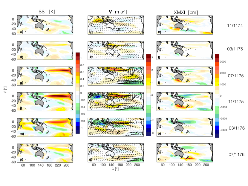
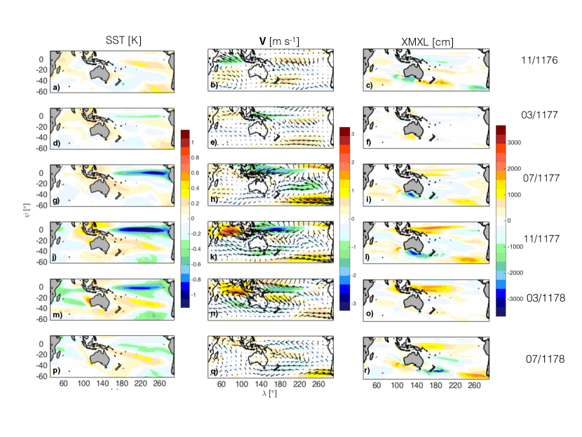
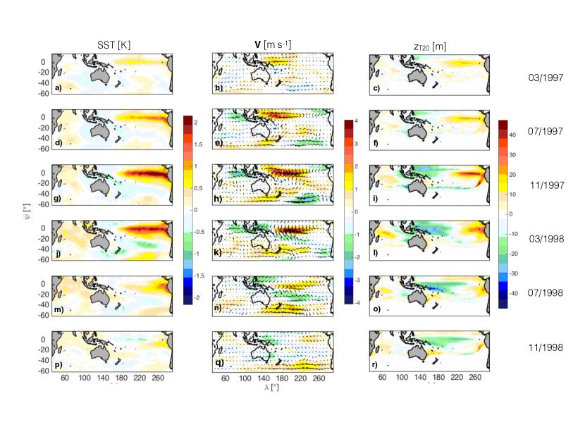
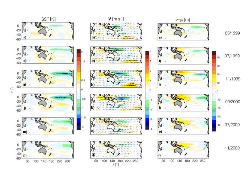
It is well known that interannual SST variability in the Pacific Ocean is strongly coupled with surface atmospheric and thermocline variability (Alexander et al. 2002; Lengaigne et al. 2006; Vecchi 2006; McGregor et al. 2012; Stuecker et al. 2013, 2015a). In this section, we examine the nature of this coupling in the context of the ENSO and ENSO-A combination modes recovered from the CCSM4 and HadISST data in Part I. In particular, we examine spatiotemporal reconstructions of SST, surface winds, and thermocline depth associated with this mode family. In what follows, we describe the properties of these reconstructions with reference to specific strong ENSO events in CCSM4 and observations, as we find that individual events are better-suited than composites for describing propagating features from the ENSO and ENSO-A modes evolving on monthly timescales. In the case of CCSM4, we focus on the simulation period 01/1170–12/1180 where ENSO activity is strong (and the WPMM is in its cold phase; see section 5). This period contains a strong El Niño event in the boreal winter of 1175–1176 followed by a strong La Niña event in the boreal winter of 1177–1188. In the case of HadISST, we focus on the period 01/1997–12/2000 containing the strong 1997–1998 El Niño and the subsequent La Niña in 1999–2000. The event from CCSM4 and HadISST are visualized in movies 1 and 2 in the supplementary material, respectively. Representative snapshots from these movies are displayed in Figs. 1–4. Due to the high temporal coherence of ENSO and ENSO-A modes, the conclusions drawn from these events are representative of other reconstructed ENSO events.
We first consider the reconstructions from CCSM4. As shown in Fig. 1 and movie 1 in the supplementary material, positive SST anomalies associated with the 1175–1176 El Niño begin building up in the eastern Pacific in FMA 1175. During that period, anomalous westerly winds develop in the western tropical Pacific, and a positive XMXL anomaly travels from the western to eastern equatorial Pacific where it continues to increase in the ensuing months. The eastern Pacific SST anomalies also increase during that time until the event peaks in November-December 1175 reaching K SST anomalies in the central-eastern equatorial Pacific. Around the time of the El Niño peak, the anomalous western Pacific westerlies undergo a pronounced southward shift to S, which is accompanied by a return of the eastern equatorial Pacific thermocline depth to near-climatological levels by July-August 1176. Meanwhile, the positive SST anomalies in the Eastern Pacific gradually decay until La Niña conditions begin developing in FMA 1177. The ensuing La Niña episode (see Fig. 2) evolves as a sign-reversed analog of the El Niño event described above.
More detailed aspects of the thermocline response due to the southward shift of meridional winds is captured in reconstructions in movie 1 in the supplementary material which are based on ENSO-A modes alone. There, it can be seen that as the anomalous westerlies shift to the south of the equator in February-March 1176, a positive XMXL anomaly is generated in the central equatorial Pacific and propagates to the west, reaching the Maritime Continent in August-September 1176 where it contributes to the return of the previously negative XMXL anomaly there to near-climatological levels. That anomaly is then reflected and begins propagating towards the East, reaching the Eastern Pacific in March–April 1177.
Overall, the atmosphere-ocean process described above is in good agreement with the predictions of ENSO combination mode theory Stein et al. (2011, 2014); McGregor et al. (2012); Stuecker et al. (2013, 2015a). In particular, using intermediate-complexity atmosphere and ocean models, McGregor et al. (2012) propose a mechanism whereby the SST anomalies from a developed ENSO event induce a Gill-type Rossby-Kelvin wave in the lower tropopause which leads to an ageostrophic boundary-layer flow. The latter is stronger in the South Pacific relative to the North Pacific due to weaker climatological wind speeds and associated Ekman pumping in DJF and MAM, giving rise to a seasonally-locked southward shift of meridional winds. Moreover, using a reduced ocean model, they propose that this southward wind shift of meridional winds causes two distinct oceanic responses involving generation of equatorial Kelvin waves or equatorial heat recharge/discharge which are responsible for terminating ENSO events. This seasonally locked southward shift of meridional winds preceding ENSO termination is well captured in Fig. 1 and 2 and movie 1 in the supplementary material. As stated in section 1 and in Part I, a representation of the southward zonal wind shift can also be obtained through the two leading EOFs of atmospheric circulation fields (McGregor et al. 2012; Stuecker et al. 2013), but this representation mixes the three distinct ENSO and ENSO-A frequencies into a single PC pair. In contrast, the NLSA eigenfunctions recovered from SST isolate the components of ENSO and ENSO-A variability through three distinct pairs of modes evolving at the correct theoretical frequencies. This more detailed and theoretically consistent decomposition should be useful for future studies of ENSO termination.
Next, we consider the SST, surface wind, and Z20 reconstructions associated with the ENSO and ENSO-A modes extracted from the observational data. As shown in Figs. 3 and 4 and movie 2 in the supplementary material, SST anomalies preceding the strong El Niño of 1997–1998 begin developing in the equatorial eastern Pacific in DJF 1996–1997 and continue growing until the event’s peak in December 1997-January 1998. The buildup of SST anomalies is accompanied by anomalous westerlies in the western Pacific and the establishment of an anomalous shallow (deep) thermocline in the western (eastern) tropical Pacific. The anomalous zonal winds migrate to the south (in a process that begins moths prior to the event peak), reaching a maximum southerly latitude of S in March 1998, at which point they start to diminish, and the SST and Z20 anomalies in the eastern Pacific decay to climatological levels. ENSO-neutral conditions are established by September 1998, and in December 1997 a La Niña event begins to emerge. The SST anomalies from that event peak in January 2000 and are accompanied by anomalous easterlies in the western Pacific and a negative zonal gradient of Z20 anomalies. The La Niña event rapidly decays in the spring of 2000 following the southward shift and decay of the anomalous easterlies.
In general, the reconstructions based on CCSM4 and observations are in good agreement over the equatorial Pacific where the majority of ENSO activity takes place—this is to be expected since CCSM4 is known to simulate realistic ENSO variability (Deser et al. 2012). A Pacific Ocean region where the observational reconstructions differ from those from CCSM4 is the Maritime Continent region north of Sumatra. There, during El Niño events the SST anomalies are positive in the observational data but negative in the CCSM4 data, and an analogous but opposite-sign discrepancy takes place during La Niña events. These discrepancies can also be seen in the composites in Figs. 9–12 in Deser et al. (2012) which are based on Niño-3.4 indices.
3.2 Pacific and Indian Ocean couplings
Besides the tropical Pacific Ocean, the ENSO and ENSO-A modes have strong surface atmospheric and thermocline response in the Indian and South Pacific Oceans. As shown in Fig. 1 and movie 1 in the supplementary material, coincident with the 1175–1176 El Niño event is the formation of a prominent anticyclonic surface circulation in the southeast Indian Ocean off the western coast of Australia (see, e.g,. the period December 1175–March 1176). This circulation pattern is consistent with the development of (i) positive SST anomalies in the western Indian Ocean (which are especially pronounced off Africa’s east coast) via advection of warm water from the Maritime Continent, and (ii) negative SST anomalies in the eastern Indian Ocean via advection of cold water from the southern Indian Ocean. This dipole SST pattern typically peaks in February, and decays together with the main El Niño SST anomalies during boreal spring. As noted in Part I, this SST pattern is characteristic of the IOD, and explains of the raw nonperiodic variance in the Indian Ocean regions used to define IOD indices (Saji et al. 1999). In the case of La Niña events (Fig. 2 and movie 1 in the supplementary material), the southeastern Indian Ocean anticyclone is replaced by a cyclone (centered at the same location), and the positive SST anomalies in the western Indian Ocean are replaced by positive SST anomalies in the eastern Indian Ocean, especially in the region west of the Sunda Strait.
In the case of observational data, significant Indian-Pacific Ocean couplings also take place during El Niño (Fig. 3) and La Niña (Fig. 4) events (see also movie 2 in the supplementary material), though with some notable differences compared to the CCSM4 data. In particular, unlike the clear dipole SST that develops in the reconstructions from the CCSM4 data during peaking El Niño/La Niña events (see, e.g, December 1175 in movie in the supplementary material), the Indian Ocean SST anomalies are of the same sign in the observational data (positive and negative during El Niños and La Niñas, respectively; see, e.g, December 1997 in movie 2 in the supplementary material), though they are generally stronger in the western part of the Indian Ocean (especially east-northeast of Madagascar), giving rise to a zonal SST gradient as in CCSM4. Instead, dipolar SST anomaly patterns with a clear sign reversal over the Indian Ocean can be seen during months preceding El Niño/La Niña peaks; e.g., July 1997 in movie 2 in the supplementary material.
3.3 El Niño-La Niña asymmetries
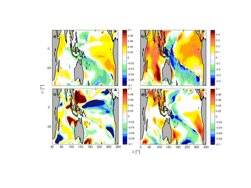
As discussed in section 5a of Part I, besides the fundamental ENSO and ENSO-A modes the NLSA spectrum can also contain “secondary” ENSO modes with frequencies adjacent to the main ENSO band. These modes form degenerate oscillatory pairs, emerging as the Takens embedding window used in NLSA is increased from interannual to decadal lengths. In particular, the embedding window used to compute modes from the CCSM4 dataset is y and a number of secondary modes are present in the spectrum; see Fig. 9 in Part I. This behavior is consistent with NLSA progressively resolving a broadband spectrum (here, due to ENSO) into distinct modes as grows (Berry et al. 2013; Giannakis 2016). In this section, we examine the role of these secondary ENSO modes in capturing the third-order statistics of ENSO, and in particular the positive SST skewness associated with strong El Niño events (Burgers and Stephenson 1999; An and Jin 2004; Weller and Cai 2013).
Figure 5(a) shows a spatial map of the normalized skewness coefficient at each gridpoint using the reconstructed SST field obtained from the fundamental ENSO modes and the family of secondary ENSO modes from CCSM4 shown in Fig 9(a) in Part I, together with their associated combination modes with the annual cycle. The normalized skewness coefficient at gridpoint is defined as , where overbars denote time averages, and and are reconstructed SST fields and their standard deviations for the selected mode family (see section 2c in Part I). In Fig. 5(a), skewness is positive over the eastern Pacific cold tongue region associated where the majority of ENSO activity occurs, and takes negative values in the western Pacific. Moreover, the Indian Ocean features a dipolar skewness pattern with predominantly positive (negative) values in the western (eastern) parts of the basin. These features are consistent with skewness patterns constructed from detrended observational SSTs (see, e.g., Fig. 6(c) in Weller and Cai 2013) (although the skewness values in Fig. 5(a) are about a factor of 10 smaller than the corresponding values from raw SSTs.) Using more secondary ENSO modes, or a shorter embedding window as illustrated in Fig.5(b), leads to higher skewness values from those shown in Fig. 5(a).
Next, to assess the contributions of the individual modes in the ENSO family used to build the map in Fig 5(a), we examine skewness maps based on either the fundamental ENSO and ENSO-A modes (Fig. 5(c)), or the secondary ENSO and ENSO-A modes (Fig. 5(d)) alone. Interestingly, the skewness maps based on the fundamental modes take negative values in the eastern Pacific cold tongue, and those based on the secondary modes are positive but much weaker there. These facts indicate that the positive skewness from the full ENSO family is an outcome of product terms between the fundamental and secondary ENSO modes. Assuming that the secondary ENSO modes are part of a ENSO frequency cascade (Stuecker et al. 2013) resolved by NLSA (as conjectured in section 5a of Part I), these results suggest that at least in CCSM4, the positive eastern Pacific SST skewness due to ENSO may be the outcome of an interaction between the fundamental and secondary frequencies in that cascade.
In the case of HadISST data, the modes were computed using a 4-year embedding window (see section 7 in Part I), and as a result a single set of ENSO and ENSO-A modes represents the ENSO variability that would be split into fundamental and secondary modes at longer embedding windows. As shown in Fig. 5(e), the normalized skewness map computed from the ENSO and ENSO-A family also recovers the basic features seen in skewness maps from raw SST data, and moreover exhibits generally higher values than the model data.
4 Atmosphere-ocean co-variability of the TBO and TBO combination modes in CCSM4
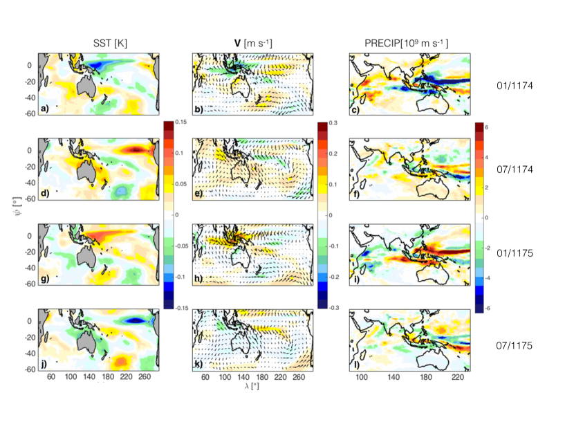
Next, we study SST, surface wind, and precipitation patterns associated with the TBO and TBO-A modes recovered from CCSM4. As in section 3, we discuss the evolution of this patterns with reference to a specific TBO event occurring in the simulation period 12/1169–12/1171. Snapshots from this period are displayed in Fig. 6, and movie 3 in the supplementary material shows the full dynamical evolution of the SST, surface wind, and precipitation fields associated with the TBO and TBO-A modes.
As shown in Fig. 6(a–c), the boreal winter of simulation year 1169 is an anomalously weak Australian monsoon year featuring horizontal surface divergence (subsidence) and negative SST anomalies over the western Pacific, and negative precipitation anomalies stretching south from the Maritime Continent to northern Australia. This warm pool divergence drives anomalous easterlies over the eastern and central Indian Ocean and anomalous westerlies over the central tropical Pacific. The anomalous easterlies correspond to a weakened western Walker Cell, enabling the development of positive SST anomalies in the western Indian Ocean and intensification of deep convection (as evidenced by positive precipitation anomalies in east Africa). Meehl and Arblaster (2002) associate this pattern with a Rossby wave response over Asia and positive temperature anomalies over the Indian subcontinent, preconditioning for a strong Indian monsoon in the upcoming boreal summer. Indeed, in JJAS 1170 an anomalously strong Indian monsoon takes place (see positive precipitation anomalies over the Indian subcontinent and Southeast Asia in Fig. 6(f)). During that time, the western Walker cell is anomalously strong (Fig. 6(e)), and anomalous precipitation occurs over the tropical eastern Indian Ocean and western Pacific driven by positive SST anomalies there (Fig. 6(d)). Meehl and Arblaster (2002) attribute the development of these anomalies to thermocline adjustment resulting from eastward-propagating Kelvin waves generated by the anomalous circulation in the preceding winter and spring months.
The positive SST anomalies in the waters off Australia and the Maritime Continent persist over the ensuing boreal fall and winter (Fig. 6(g)). As a result, as precipitation gradually shifts southeastward from India and Southeast Asia in response to the annual cycle of insolation, it becomes anomalously strong. This results in an anomalously strong Australian monsoon in the boreal winter of 1170–1171 (Fig. 6(i)), completing the first half of the TBO cycle. In 1171–1172, the mechanism described above is effectively sign-reversed, and an anomalously week Indian Monsoon takes place (Fig. 6(j–l), followed by a weak Australian monsoon in the boreal winter of 1172–1173 (not shown), completing the TBO cycle.
In summary, we find that in CCSM4 the spatiotemporal SST, precipitation, and surface wind patterns represented by the TBO and TBO-A modes are broadly consistent with the mechanism for biennial monsoon variability proposed by Meehl and Arblaster (2002). It is important to note that as with ENSO, both the fundamental and combination (TBO-A) modes are essential in representing this seasonally-locked process, but due to the weak ( K) SST anomalies involved, these modes are challenging to capture from unprocessed observational data. In Part I we saw that it was possible to recover via NLSA modes resembling the TBO (albeit with mixing between the fundamental and combination frequencies) from HadISST data spanning the industrial era, but not the satellite era for which reliable reanalysis data are available. Nevertheless, longer historical datasets are available for certain variables relevant to the TBO such as Indian rainfall (Rajeevan et al. 2006), and it should be an interesting topic for future work to study such datasets using the modes recovered here from industrial-era HadISST in studies of the TBO.
5 Decadal-interannual interactions and climatic impacts in CCSM4
5.1 Amplitude modulation of ENSO and the TBO
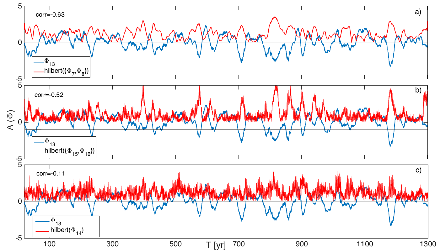
In this section, we examine the modulating relationships between the WPMM and other interannual and decadal modes in the NLSA spectrum. Figure 7 displays the temporal pattern corresponding to the WPMM, together with the amplitude envelopes of the fundamental ENSO modes, the TBO modes, and the IPO mode recovered from the CCSM4 data (see section 4 in Part I). There, one can clearly notice that the envelopes of the fundamental ENSO modes and the biennial modes correlate negatively and significantly with the temporal pattern of the WPMM. In particular, the correlation coefficients equal and , respectively for ENSO and the TBO. Moreover, it is evident that the nature of these modulating relationships is sign-dependent, in the sense that strengthening of the interannual modes occurs predominantly during negative phases of WPMM, i.e., during negative SST anomalies in the western tropical Pacific. On the other hand, the correlations between the amplitudes of the IPO-like mode and the WPMM are significantly weaker (with a correlation coefficient of ; see Fig. 7(c)). Similarly weak correlations are also observed between the IPO-like modes and the amplitudes of the dominant ENSO and biennial modes.
We note that in the case of the modes recovered from CM3 (see section 6 in Part I), we also observe amplitude modulation relationships (not shown here) between the WPMM and the interannual modes, but these relationships are somewhat different than in CCSM4. In particular, we find that in CM3 the negative phase of the multidecadal fool correlates with increased ENSO and TBO amplitude, but during the positive WPMM phase there is no significant ENSO and TBO amplitude suppression as observed in CCSM4. As a result, the corresponding time-averaged correlation coefficients are about a factor of two smaller than the CCSM4 results in Fig. 7. Another contributing factor in this decrease of correlation is that the temporal patterns of the WPMM and TBO in CM3 are noisier than in CCSM4.
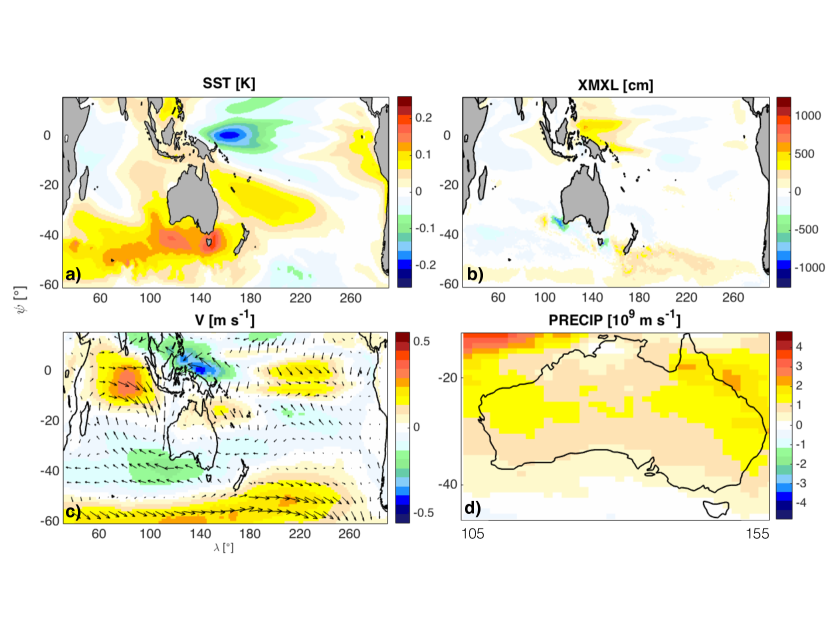
To physically account for the amplitude modulation role of the WPMM, we examine its associated reconstructed SST, surface wind, XMXL patterns, and precipitation patterns. As with ENSO and the TBO, we discuss these patterns with reference to a specific event, namely a cold WPMM event taking place during simulation years 1165–1185 (note that this interval includes the intervals employed in sections 3 and 4 in our discussion of ENSO and TBO, respectively). The 1165–1185 cold WPMM event is illustrated through composites in Fig. 8, and can be directly visualized in movie 3 in the online supplementary material. There, it is evident that during the WPMM’s cold phase, the decadal cluster of negative SST anomalies in the West Pacific is collocated with surface wind divergence, leading to anomalous westerlies in the central and eastern Pacific and anomalous easterlies in the western Pacific region north of the Maritime Continent. The thermocline depth associated with the cold WPMM phase features strong positive anomalies in the western Pacific region collocated with the anomalous easterlies, but also exhibits appreciable negative and positive anomalies in the central and eastern Pacific, respectively. Together, these patterns create a flatter meridional thermocline profile, and such conditions have been shown to correlate with periods of stronger ENSO variability (Kirtman and Schopf 1998; Kleeman et al. 1999; Fedorov and Philander 2000; Rodgers et al. 2004). In addition, the cold ENSO phase features a prominent cyclonic circulation over the Indian Ocean (centered at S and E) which strengthens the western Walker cell and advects warm, moist air from the Maritime Continent towards northern Australia. These conditions are favorable to the Australian monsoon, and thus may explain the observed TBO strengthening during cold WPMM phases.
Besides the tropical Pacific Ocean, the WPMM has a coherent atmospheric circulation signature in the Indian and Southern Oceans. In the Indian Ocean, the cold phase of the WPMM is associated with a prominent anticyclonic gyre centered in the central-eastern Indian ocean at S latitudes. Advection from this gyre is consistent with the dipole of SST anomalies in the Indian Ocean featuring positive (negative) SST anomalies in the eastern (western) part of the basin. In the South Pacific and south Indian Ocean, the WPMM creates a coherent pattern of anomalous easterlies spanning the full meridional extent of the Indo-Pacific basin.
5.2 Decadal precipitation over Australia
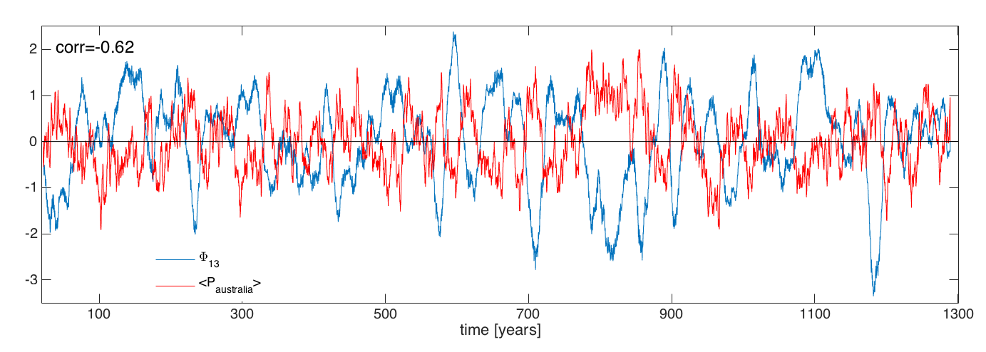
The precipitation composites in Fig. 8(d) suggest that the WPMM plays an important modulating role in the multidecadal variability of Australian precipitation as simulated by CCSM4. To assess the strength of this relationship we examine the 11-year running average of spatially averaged precipitation data over Australia computed from the 1300 y CCSM4 control run. Figure 9 shows the resulting millennial time series, , along with the temporal pattern associated with the WPMM. As with the WPMM, pronounced fluctuations of occur on multidecadal timescales, and the correlation coefficient between the two time series is . In particular, negative phases of the WPMM (i.e., negative SST anomalies over the western tropical Pacific and positive SST anomalies to the south of Australia) are associated with anomalously wet periods that can last almost a century, and positive phases result in prolonged droughts. For comparison, the correlation coefficient between and the temporal pattern of the IPO (not shown here), obtained through the first EOF of 13 y running mean of CCSM4 Indo-Pacific SST data after linear detrending to remove model drift, is 0.44.
As shown in Fig. 8(d), the cold WPMM phase is associated with precipitation enhancement over the whole Australian continent. In the north, this convective intensification is dynamically consistent with the surface atmospheric winds entraining anomalously warm and moist air, which is driven primarily by subsiding circulation and divergent air motion centered over the anomalously cold western Pacific SST. Moreover, additional enhancement of precipitation can be attributed to thermodynamic factors such as positive SST anomalies off the Australian coast that surround the whole continent and are particularly pronounced over its southern part. Of course, given the deficiencies of global climate models in simulating precipitation, we cannot claim that the modulating relationships between the WPMM and decadal Australian precipitation identified in CCSM4 also apply in nature. Nevertheless, these results demonstrate that at least for the climate simulated by CCSM4 the WPMM is a physically meaningful mode, and provide motivation for seeking analogous patterns and mechanisms in the real climate system.
6 Concluding remarks
In this paper, we have employed a family of modes identified via NLSA in Part I of this work (Slawinska and Giannakis 2016) to study various aspects of coupled atmosphere-ocean variability in the Indo-Pacific sector of model and observational datasets on interannual to decadal timescales. One of our main objectives has been to study the SST, surface wind, and thermocline depth patterns associated with a family of ENSO modes and combination modes between ENSO and the annual cycle (denoted ENSO-A modes), which were recovered in Part I from unprocessed Indo-Pacific SST data. We found that in both model and observational data these patterns are in good agreement with mechanisms proposed for the phase synchronization between ENSO and the seasonal cycle (Stein et al. 2011, 2014; Stuecker et al. 2013, 2015a; McGregor et al. 2012), whereby quadratic nonlinearities in the governing equations for the coupled atmosphere-ocean system lead to a seasonally-dependent southward shift of zonal winds following the boreal winter peak of El Niño (La Niña) events, generating an upwelling oceanic response restoring the ENSO state to neutral or La Niña (El Niño) conditions. We also showed that the surface wind patterns associated with the ENSO and ENSO-A modes produce a coupling between the Indian and Pacific ocean SST with SST patterns resembling the IOD. This relationship is purely deterministic, suggesting that the ENSO and ENSO-A modes are good predictors for IOD variability.
Besides ENSO, we studied the SST, surface wind, and precipitation patterns associated with a family of biennial modes and biennial-annual combination modes representing the TBO in CCSM4. We showed that despite the small SST anomalies involved (about an order of magnitude smaller than typical ENSO amplitudes), these patterns are consistent with coupled atmosphere-ocean mechanisms for biennial variability of the Asian-Australian monsoon (Meehl and Arblaster 2002), whereby an anomalously week Australian monsoon in boreal winter tends to be followed by anomalously strong Indian and Australian monsoons in the ensuing boreal summer and winter. Given that our TBO modes were recovered without bandpass filtering the input data, these results support the existence of the TBO as an intrinsic, physically meaningful process that can be consistently inferred from SST data alone (at least in CCSM4), although our analysis does not address the causality relationships between it and other modes of climate variability such as ENSO (Goswami 1995; Meehl and Arblaster 2002; Li et al. 2006; Meehl and Arblaster 2011). In Part I, we were less successful in identifying coherent TBO patterns in model and observational SST datasets other than the millenial control integration of CCSM4 studied here (corroborating similar difficulties faced by other studies; e.g., Stuecker et al. 2015b), but the encouraging results from CCSM4 suggest expanding this study to other datasets and/or including additional physical variables that would improve the detectability of TBO patterns.
In the decadal timescale, we studied amplitude modulation relationships between the WPMM (the dominant mode of Indo-Pacific multidecadal variability recovered by NLSA from CCSM4 data in Part I, featuring a prominent cluster of SST anomalies in the west-central Pacific) with ENSO, the TBO, and decadal precipitation over Australia. We found that the WPMM exhibits a significant anticorrelation with the decadal envelope of ENSO and the TBO (at the and level, respectively), with cold (warm) WPMM phases corresponding to decadal periods of enhanced (suppressed) ENSO activity. In particular, we showed that cold WPMM periods are associated with anomalous westerlies in the central equatorial Pacific and anomalously deep thermocline in the eastern Pacific, leading to a background configuration which previous studies have shown to favor ENSO activity and predictability (Kirtman and Schopf 1998; Kleeman et al. 1999; Fedorov and Philander 2000; Rodgers et al. 2004). We also demonstrated that cold WPMM phases can favor Australian monsoon activity through anomalous westerlies in the Indian Ocean strengthening the western Walker Cell, which may explain the enhanced TBO activity during those periods. Moreover, we showed that the WPMM anticorrelates significantly (at the -0.6 level) with decadal precipitation over Australia, and justified this correlation on the basis of advection of warm moist air over the Australian continent by the atmospheric circulation patterns associated with the WPMM. Thus, at least in the model data studied here, the WPMM is a good predictor of prolonged droughts and/or anomalously wet periods there. Overall, even though we were not able to robustly recover the WPMM from observational data (in Part I, we only found tentative evidence for this mode in industrial-era HadISST data), our results from CCSM4 allude to it being an important pattern of Indo-Pacific variability which could potentially be useful in conjunction with the IPO to characterize the decadal behavior of the real climate.
In summary, the family of NLSA modes identified in this work provide an attractive low-dimensional basis to characterize numerous features of the Indo-Pacific climate system. Potential future applications of these modes include objective and accurate ways of indexing oceanic oscillations across multiple timescales, studies of statistical and causal dependencies and their underlying physical mechanisms in the coupled atmosphere-ocean system, as well predictive models based on these modes to assess future climate fluctuations from interannual to multidecadal horizons. From a data analysis standpoint this work has demonstrated that nonlinear kernel methods, appropriately designed to take dynamics into account, can potentially overcome some of the limitations of classical linear techniques in revealing intrinsic modes of multidecadal climate variability, but our study is certainly only an initial step in this direction. Further assessment and refinement of the patterns identified here should be a fruitful avenue for future work.
Acknowledgements.
J. Slawinska received support from the Center for Prototype Climate Modeling at NYU Abu Dhabi and NSF grant AGS-1430051. The research of D. Giannakis is supported by ONR Grant N00014-14-0150, ONR MURI Grant 25-74200-F7112, and NSF Grant DMS-1521775. We thank Sulian Thual for stimulating conversations and three anonymous reviewers for comments that helped significantly improve the paper. This research was partially carried out on the high performance computing resources at New York University Abu Dhabi.References
- Alexander et al. (2002) Alexander, M. A., I. Bladé, M. Newman, J. R. Lanzante, N.-C. Lau, and J. D. Scott, 2002: The atmospheric bridge: The influence of ENSO teleconnections on air–sea interaction over the global oceans. J. Climate, 15, 2205–2231, 10.1175/1520-0442(2002)0152205:TABTIO2.0.co;2.
- An and Jin (2004) An, S.-I., and F.-F. Jin, 2004: Nonlinearity and asymmetry of ENSO. J. Climate, 17, 2399–2412, 10.1175/1520-0442(2004)017¡2399:NAAOE¿2.0.CO;2.
- An et al. (2004) An, S.-I., A. Timmermann, L. Bejarano, F.-F. Jin, F. Justino, Z. Liu, and A. W. Tudhope, 2004: Modeling evidence for enhanced El Niño Southern Oscillation amplitude during the Last Glacial Maximum. Paleoceanography, PA4009, 10.1029/2004PA001020.
- Annamalai et al. (2003) Annamalai, H., R. Murtugudde, J. Potemra, S. P. Xie, P. Liu, and B. Wang, 2003: Coupled dynamics in the Indian Ocean: Spring initiation of the zonal mode. Deep-Sea Res., 50, 2305–2330, 10.1016/S0967-0645(03)00058-4.
- Barnett et al. (1999) Barnett, T. P., D. W. Pierce, M. Latif, D. Dommenget, and R. Saravanan, 1999: Interdecadal interactions between the tropics and midlatitudes in the Pacific Basin. Geophys. Res. Lett., 26 (5), 615––618, 10.1029/1999GL900042.
- Berry et al. (2013) Berry, T., R. Cressman, Z. Greguric Ferencek, and T. Sauer, 2013: Time-scale separation from diffusion-mapped delay coordinates. SIAM J. Appl. Dyn. Sys., 12, 618–649, 10.1137/12088183X.
- Bjerknes (1969) Bjerknes, J., 1969: Atmospheric teleconnections from the equatorial Pacific. Mon. Wea. Rev., 97 (3), 163–172, 10.1175/1520-0493(1969)097¡0163:ATFTEP¿2.3.CO;2.
- Burgers and Stephenson (1999) Burgers, G., and D. B. Stephenson, 1999: The “normality” of El Niño. Geophys. Res. Lett., 26 (8), 1027–1030, 10.1175/1520-0442(2004)017¡2399:NAAOE¿2.0.CO;2.
- C-GLORS (2014) C-GLORS, 2014: Cmcc global ocean physical reanalysis system (c-glors025v4.1) data. Centro Euro-Mediterraneo sui Cambiamenti Climatici, URL: http://www.cmcc.it/c-glors/, accessed July 2016.
- Cane et al. (1995) Cane, M. A., S. Zebiak, and Y. Xue, 1995: Model studies of the long-term behavior of ENSO. Natural Climate Variability on Decade-to-Century Time Scales, D. G. M. et al., Ed., National Academy Press, Washington, D.C., Vol. DEC-CEN Workshop, Irvine, CA, 442–457.
- CCSM (2010) CCSM, 2010: Community Climate System Model Version 4 (CCSM4) data. Earth System Grid at the National Center for Atmospheric Research, URL: https://www.earthsystemgrid.org/dataset/ucar.cgd.ccsm4.joc.b40.1850.track1.1deg.006.html, last accessed August 2016.
- Choi et al. (2009) Choi, J., S.-I. An, B. Dewitte, and H. W. W., 2009: Interactive feedback between the tropical Pacific Decadal Oscillation and ENSO in a Coupled General Circulation Model. J. Climate, 22, 6597–6611.
- Choi et al. (2012) Choi, J., S.-I. An, and S.-W. Yeh, 2012: Decadal amplitude modulation of two types of ENSO and its relationship with the mean state. Clim. Dyn., 38, 2631–2644, 10.1007/s00382-011-1186-y.
- Dai (2013) Dai, A., 2013: The influence of the inter-decadal Pacific oscillation on U.S. precipitation during 1923-2010. Climate Dyn., 41, 633–646, 10.1007/s00382-012-1446-5.
- Deser et al. (2010) Deser, C., M. A. Alexander, S.-P. Xie, and A. S. Phillips, 2010: Sea Surface Temperature Variability: Patterns and Mechanisms. Annual Review of Marine Science, 2, 115–143, 10.1146/annurev-marine-120408-151453.
- Deser et al. (2012) Deser, C., A. S. Phillips, R. A. Tomas, Y. M. Okumura, M. A. Alexander, A. Capotondi, and J. D. Scott, 2012: ENSO and Pacific decadal variability in the Community Climate System Model Version 4. J. Climate, 25, 2622–2651, 10.1175/JCLI-D-11-00301.1.
- England et al. (2015) England, M. H., J. B. Kajtar, and N. Maher, 2015: Robust warming projections despite the recent hiatus. Nature Clim. Change, 5, 394–396, 10.1038/nclimate2575.
- England et al. (2014) England, M. H., and Coauthors, 2014: Recent intensification of wind-driven circulation in the Pacific and the ongoing warming hiatus. Nat. Clim. Change, 4, 222–227, 10.1038/nclimate2106.
- Fedorov and Philander (2000) Fedorov, A. V., and G. S. Philander, 2000: Is el niño changing? Science, 288 (5473), 1997–2002, 10.1126/science.288.5473.1997.
- Gent et al. (2011) Gent, P. R., and Coauthors, 2011: The Community Climate System Model version 4. J. Climate, 4973–4991, 10.1175/2011jcli4083.1.
- Giannakis (2015) Giannakis, D., 2015: Dynamics-adapted cone kernels. SIAM J. Appl. Dyn. Sys., 14 (2), 556–608, 10.1137/140954544.
- Giannakis (2016) Giannakis, D., 2016: Data-driven spectral decomposition and forecasting of ergodic dynamical systems. 1507.02338.
- Giannakis and Majda (2011) Giannakis, D., and A. J. Majda, 2011: Time series reconstruction via machine learning: Revealing decadal variability and intermittency in the North Pacific sector of a coupled climate model. Conference on Intelligent Data Understanding 2011, Mountain View, California.
- Giannakis and Majda (2012a) Giannakis, D., and A. J. Majda, 2012a: Comparing low-frequency and intermittent variability in comprehensive climate models through nonlinear Laplacian spectral analysis. Geophys. Res. Lett., 39, L10 710, 10.1029/2012GL051575.
- Giannakis and Majda (2012b) Giannakis, D., and A. J. Majda, 2012b: Nonlinear Laplacian spectral analysis for time series with intermittency and low-frequency variability. Proc. Natl. Acad. Sci., 109 (7), 2222–2227, 10.1073/pnas.1118984109.
- Giannakis and Majda (2013) Giannakis, D., and A. J. Majda, 2013: Nonlinear Laplacian spectral analysis: Capturing intermittent and low-frequency spatiotemporal patterns in high-dimensional data. Stat. Anal. Data Min., 6 (3), 180–194, 10.1002/sam.11171.
- Giannakis and Majda (2014) Giannakis, D., and A. J. Majda, 2014: Data-driven methods for dynamical systems: Quantifying predictability and extracting spatiotemporal patterns. Mathematical and Computational Modeling: With Applications in Engineering and the Natural and Social Sciences, R. Melnik, Ed., Wiley, Hoboken, 288.
- Goswami (1995) Goswami, B. N., 1995: A multiscale interaction model for the origin of the tropspheric QBO. J. Climate, 8, 524–534, 10.1175/1520-0442(1995)008¡0524:AMIMFT¿2.0.CO;2.
- Griffies et al. (2011) Griffies, S. M., and Coauthors, 2011: The GFDL CM3 coupled climate model: Characteristics of the ocean and sea ice simulations. J. Climate, 24, 3520–3544, 10.1175/2011JCLI3964.1.
- Gu and Philander (1997) Gu, D., and S. G. H. Philander, 1997: Interdecadal Climate Fluctuations That Depend on Exchanges Between the Tropics and Extratropics. Science, 275, 805–807, 10.1126/science.275.5301.805.
- HadISST (2013) HadISST, 2013: Hadley Centre Sea Ice and Sea Surface Temperature (HadISST1) data. Met Office Hadley Centre, URL: http://www.metoffice.gov.uk/hadobs/hadisst/data/download.html, accessed June 2015.
- Han et al. (2014) Han, W., and Coauthors, 2014: Intensification of decadal and multi-decadal sea level variability in the western tropical Pacific during recent decades. Climate Dyn., 4, 1357–1379, 10.1007/s00382-013-1951-1.
- Hasegawa and Hanawa (2006) Hasegawa, T., and K. Hanawa, 2006: Impact of quasi-decadal variability in the tropical Pacific on ENSO modulations. J. Oceanogr., 62, 227–234, 10.1007/s10872-006-0047-5.
- Imada and Kimoto (2009) Imada, Y., and M. Kimoto, 2009: ENSO amplitude modulation related to Pacific decadal variability. Geophys. Res. Lett., 36, L03 706, 10.1029/2008GL036421.
- Karnauskas et al. (2009) Karnauskas, K. B., R. Seager, A. Kaplan, Y. Kushnir, and M. A. Cane, 2009: Observed Strengthening of the Zonal Sea Surface Temperature Gradient across the Equatorial Pacific Ocean. J. Climate, 22 (16), 4316–4321, 10.1175/2009JCLI2936.1.
- Kirtman and Schopf (1998) Kirtman, B. P., and P. S. Schopf, 1998: Decadal variability in ENSO predictability and prediction. J. Climate, 11, 2804–2822, 10.1175/1520-0442(1998)011¡2804:DVIEPA¿2.0.CO;2.
- Kleeman et al. (1999) Kleeman, R., J. P. McCreary, Jr., and B. A. Klinger, 1999: A mechanism for generating ENSO and Decadal variability. Geophys. Res. Lett., 26, 1743–1746, 10.1029/1999gl900352.
- Knutson and Manabe (1998) Knutson, T. R., and S. Manabe, 1998: Model Assessment of Decadal Variability and Trends in the Tropical Pacific Ocean. J. Climate, 11, 2273–2296, http://dx.doi.org/10.1175/1520-0442(1998)011¡2273:MAODVA¿2.0.CO;2.
- Lengaigne et al. (2006) Lengaigne, M., J.-P. Boulanger, C. Menkes, and H. Spencer, 2006: Influence of the seasonal cycle on the termination of El Niño events in a Coupled General Circulation Model. J. Climate, 19, 1850–1868, dx.doi.org/10.1175/JCLI3706.1.
- Li (2013) Li, T., 2013: Monsoon Climate Variabilities, 27–51. American Geophysical Union, 10.1029/2008GM000782, URL http://dx.doi.org/10.1029/2008GM000782.
- Li et al. (2006) Li, T., P. Liu, X. Fu, B. Wang, and G. A. Meehl, 2006: Spatiotemporal Structures and Mechanisms of the Tropospheric Biennial Oscillation in the Indo-Pacific Warm Ocean Regions. J. Climate, 19, 3070–3087, http://dx.doi.org/10.1175/JCLI3736.1.
- Li and Zhang (2002) Li, T., and Y. Zhang, 2002: Processes that determine the quasi-biennial and lower-frequency variability of the south asian monsoon. Journal of the Meteorological Society of Japan. Ser. II, 80 (5), 1149–1163, 10.2151/jmsj.80.1149.
- Liu et al. (2002) Liu, Z., L. Wu, R. Gallimore, and R. Jacob, 2002: Search for the origins of Pacific decadal climate variability. Geophys. Res. Lett., 29 (10), 42.1–42.4, 10.1029/2001GL013735.
- Luo et al. (2012) Luo, J. J., W. Sasaki, and Y. Masumoto, 2012: Indian Ocean warming modulates Pacific climate change. Proc. Natl. Acad. Sci., 109, 18 701–18 706, 10.1073/pnas.1210239109.
- Mantua et al. (1997) Mantua, N. J., S. R. Hare, Y. Zhang, J. M. Wallace, and R. Francis, 1997: A Pacific Interdecadal Climate Oscillation with Impacts on Salmon Production. Bull. Amer. Meteor. Soc., 78, 1069–1079, http://dx.doi.org/10.1175/1520-0477(1997)078¡1069:APICOW¿2.0.CO;2.
- McGregor et al. (2012) McGregor, S., A. Timmermann, N. Schneider, M. F. Stuecker, and M. F. England, 2012: The effect of the South Pacific convergence zone on the termination of El Niño events and the meridional asymmetry of ENSO. J. Climate, 25, 5566–5586, 10.1175/JCLI-D-11-00332.1.
- Meehl (1987) Meehl, G. A., 1987: The annual cycle and interannual variability in the tropical Pacific and Indian Ocean regions. Mon. Wea. Rev., 115, 27–50, 10.1175/1520-0493(1987)115¡0027:TACAIV¿2.0.CO;2.
- Meehl (1993) Meehl, G. A., 1993: A Coupled Air-Sea Biennial Mechanism in the Tropical Indian and Pacific Regions: Role of the Ocean. J. Climate, 6, 31–41, 10.1175/1520-0442(1993)006¡0031:ACASBM¿2.0.CO;2.
- Meehl (1994) Meehl, G. A., 1994: Coupled land-ocean-atmosphere processes and South Asian Monsoon variability. Science, 266, 263–267, 10.1126/science.266.5183.263.
- Meehl (1997) Meehl, G. A., 1997: The South Asian Monsoon and the Tropospheric Biennial Oscillation. J. Climate, 10, 1921–1943, 10.1175/1520-0442(1997)010¡1921:TSAMAT¿2.0.CO;2.
- Meehl and Arblaster (2002) Meehl, G. A., and J. M. Arblaster, 2002: The tropospheric biennial oscillation and Asian–Australian monsoon rainfall. J. Climate, 15, 722–744, 10.1175/1520-0442(2002)015¡0722:TTBOAA¿2.0.CO;2.
- Meehl and Arblaster (2011) Meehl, G. A., and J. M. Arblaster, 2011: Decadal Variability of Asian-Australian Monsoon-ENSO-TBO Relationships. J. Climate, 24, 4925–4940, 10.1175/2011JCLI4015.1.
- Meehl and Arblaster (2012) Meehl, G. A., and J. M. Arblaster, 2012: Relating the strength of the tropospheric biennial oscillation (TBO) to the phase of the Interdecadal Pacific Oscillation (IPO). Geophys. Res. Lett, 39, L20 716, 10.1029/2012GL053386.
- Meehl and Hu (2006) Meehl, G. A., and A. Hu, 2006: Megadroughts in the Indian Monsoon Region and Southwest North America and a Mechanism for Associated Multidecadal Pacific Sea Surface Temperature Anomalies. J. Climate, 19, 1605–1623, 10.1175/JCLI3675.1.
- Meehl et al. (2013) Meehl, G. A., A. Hu, J. M. Arblaster, J. Fasullo, and K. E. Trenberth, 2013: Externally Forced and Internally Generated Decadal Climate Variability Associated with the Interdecadal Pacific Oscillation. J. Climate, 26, 7298–7310, 10.1175/JCLI-D-12-00548.1.
- MERRA (2014) MERRA, 2014: Modern-Era Retrospective Analysis for Research and Applications (merra) data. NASA Global Modeling and Assimilation Office, URL: https://gmao.gsfc.nasa.gov/merra/, accessed June 2016.
- Meyssignac et al. (2012) Meyssignac, B., D. Salas y Melia, M. Becker, W. Llovel, and A. Cazenave, 2012: Tropical Pacific spatial trend patterns in observed sea level: internal variability and/or anthropogenic signature? Clim. Past, 8, 787–802, 10.5194/cp-8-787-2012.
- Neelin et al. (1998) Neelin, J. D., D. S. Battisti, A. C. Hirst, F.-F. Jin, Y. Wakata, T. Yamagata, and S. E. Zebiak, 1998: ENSO theory. J. Geophys. Res., 103 (C7), 14 261––14 290, 10.1029/97JC03424.
- Newman et al. (2015) Newman, M., and Coauthors, 2015: The Pacific Decadal Oscillation, revisited. J. Climate, 29, 4399–4427, 10.1175/JCLI-D-15-0508.1.
- Ogata et al. (2013) Ogata, T., S.-P. Xie, A. Wittenberg, and D.-Z. Sun, 2013: Interdecadal Amplitude Modulation of El Niño Southern Oscillation and Its Impact on Tropical Pacific Decadal Variability. J. Climate, 26, 7280–7297, 10.1175/JCLI-D-12-00415.1.
- Okumura (2013) Okumura, Y. M., 2013: Origins of Tropical Pacific Decadal Variability: Role of Stochastic Atmospheric Forcing from the South Pacific. J. Climate, 26, 9791–9796, http://dx.doi.org/10.1175/JCLI-D-13-00448.1.
- Philander (1990) Philander, G. S., 1990: El Niño, La Niña, and the Southern Oscillation, International Geophysics, Vol. 46. Academic Press, San Diego.
- Pierce et al. (2000) Pierce, D. W., T. P. Barnett, and M. Latif, 2000: Connections between the Pacific Ocean Tropics and Midlatitudes on Decadal Timescales. J. Climate, 13, 1173–1194, http://dx.doi.org/10.1175/1520-0442(2000)013¡1173:CBTPOT¿2.0.CO;2.
- Power et al. (1999) Power, S., C. Casey, C. Folland, A. Colman, and V. Mehta, 1999: Inter-decadal modulation of the impact of ENSO on Australia. Climate Dyn., 15, 319–324, 10.1007/s003820050284.
- Rajeevan et al. (2006) Rajeevan, M., J. Bhate, J. D. Kale, and B. Lal, 2006: High resolution daily gridded rainfall data for the Indian region: Analysis of break and active monsoon spells. Curr. Sci., 91 (3), 296–306.
- Rasmusson and Carpenter (1982) Rasmusson, R. M., and T. H. Carpenter, 1982: Variations in tropical sea surface temperature and surface wind fields associated with the Southern Oscillation/El Niño. Mon. Wea. Rev., 110, 354–384, 10.1175/1520-0493(1982)110¡0354:VITSST¿2.0.CO;2.
- Rayner et al. (2003) Rayner, N. A., and Coauthors, 2003: Global analyses of sea surface temperature, sea ice, and night marine air temperature since the late nineteenth century. J. Geophys. Res., 108 (D14), 10.1029/2002jd002670.
- Ren et al. (2016) Ren, H.-L., J. Zuo, F.-F. Jin, and M. F. Stuecker, 2016: ENSO and annual cycle interaction: the combination mode representation in CMIP5 models. Clim. Dyn., 46, 3753–3765, 10.1007/s00382-015-2802-z.
- Rienecker et al. (2011) Rienecker, M. M., and Coauthors, 2011: MERRA: NASA’s Modern-Era Retrospective Analysis for Research and Applications. J. Climate, 24, 3624–3648, doi:10.1175/JCLI-D-11-00015.1.
- Rodgers et al. (2004) Rodgers, K. B., P. Friederichs, and M. Latif, 2004: Tropical Pacific Decadal Variability and Its Relation to Decadal Modulations of ENSO. J. Climate, 17, 3761–3774, http://dx.doi.org/10.1175/1520-0442(2004)017¡3761:TPDVAI¿2.0.CO;2.
- Saji et al. (1999) Saji, H. N., B. N. Goswami, P. N. Vinayachandran, and T. Yamagata, 1999: A dipole mode in the tropical Indian Ocean. Nature, 401, 360–363, 10.1038/43854.
- Salinger et al. (2001) Salinger, M. J., J. A. Renwick, and A. B. Mullan, 2001: Interdecadal Pacific Oscillation and South Pacific climate. Int. J. Climatol., 21, 1705–1721, 10.1002/joc.691.
- Sarachik and Cane (2010) Sarachik, E. S., and M. A. Cane, 2010: The El Niño-Southern Oscillation Phenomenon. Cambridge University Press, Cambridge.
- Seager et al. (2015) Seager, R., M. Hoerling, S. Schubert, H. Wang, B. Lyon, A. Kumar, J. Nakamura, and N. Henderson, 2015: Causes of the 2011-14 California Drought. J. Climate, 28 (18), 6997–7024, doi: 10.1175/JCLI-D-14-00860.1.
- Silva et al. (2011) Silva, G. A. M., A. Drumond, and T. Ambrizzi, 2011: The impact of El Niño on South American summer climate during different phases of the Pacific Decadal Oscillation. Theor. Appl. Climatol., 106, 307–319, 10.1007/s00704-011-0427-7.
- Slawinska and Giannakis (2016) Slawinska, J., and D. Giannakis, 2016: Indo-Pacific variability on seasonal to multidecadal timescales. Part I: Intrinsic sst modes in models and observations. J. Climate, submitted.
- Solomon et al. (2003) Solomon, A., J. P. McCreary, R. Kleeman, and B. A. Klinger, 2003: Interannual and Decadal Variability in an Intermediate Coupled Model of the Pacific Region. J. Climate, 16, 383–405, http://dx.doi.org/10.1175/1520-0442(2003)016¡0383:IADVIA¿2.0.CO;2.
- Solomon and Newman (2012) Solomon, A., and M. Newman, 2012: Reconciling disparate twentieth-century Indo-Pacific ocean temperature trends in the instrumental record. Nature Clim. Change, 2 (9), 691–699, 10.1038/nclimate1591.
- Stein et al. (2011) Stein, K., A. Timmermann, and N. Schneider, 2011: Phase synchronization of the El Niño-Southern Oscillation with the Annual Cycle. Phys. Rev. Lett., 107, 128 501, 10.1103/PhysRevLett.107.128501.
- Stein et al. (2014) Stein, K., A. Timmermann, N. Schneider, F.-F. Jin, and F.-F. Stuecker, 2014: ENSO Seasonal Synchronization Theory. J .Cilmate, 27, 5286–5310, 10.1175/JCLI-D-13-00525.1.
- Storto et al. (2016) Storto, A., S. Masina, and A. Navarra, 2016: Evaluation of the CMCC eddy-permitting global ocean physical reanalysis system (C-GLORS, 1982–-2012) and its assimilation components. Q. J. Roy. Meteorol. Soc., 142, 738–758, 10.1002/qj.2673.
- Stuecker et al. (2015a) Stuecker, M. F., F. Jin, and A. Timmermann, 2015a: El Niño–Southern Oscillation frequency cascade. Proc. Natl. Acad. Sci., 112 (44), 13 490–13 495, 10.1073/pnas.1508622112.
- Stuecker et al. (2015b) Stuecker, M. F., A. Timmermann, and F.-F. Jin, 2015b: Tropospheric biennial oscillation (tbo) indistinguishable from white noise. Geophys. Res. Lett., 42, 7785–7791, 10.1002/2015GL065878.
- Stuecker et al. (2013) Stuecker, M. F., A. Timmermann, F.-F. Jin, S. McGregor, and H.-L. Ren, 2013: A combination mode of the annual cycle and the El Niño/Southern Oscillation. Nat. Geosci., 6, 540–544, 10.1038/NGEO1826.
- Sun et al. (2014) Sun, D. Z., T. Zhang, Y. Sun, and Y. Yu, 2014: Rectification of El Niño–Southern Oscillation into climate anomalies of decadal and longer time scales: Results from forced ocean GCM experiments. J. Climate, 27, 2545–2561, 10.1175/JCLI-D-13-00390.1.
- Sun and Yu (2009) Sun, F., and J.-Y. Yu, 2009: A 10–15-yr modulation cycle of ENSO intensity. J. Climate, 22, 1718–1735, 10.1175/2008JCLI2285.1.
- Thompson and Battisti (2001) Thompson, C. J., and D. S. Battisti, 2001: A linear stochastic dynamical model of ENSO. Part II: Analysis. J. Climate, 14, 445–466, 10.1175/1520-0442(2001)014¡0445:ALSDMO¿2.0.CO;2.
- Timmermann (2003) Timmermann, A., 2003: Decadal ENSO amplitude modulations: A nonlinear paradigm. Global Planet. Change, 37, 135–156, 10.1016/S0921-8181(02)00194-7.
- Timmermann et al. (1999) Timmermann, A., J. Oberhuber, A. Bacher, M. Esch, M. Latif, and E. Roeckner, 1999: Increased El Niño frequency in a climate model forced by future greenhouse warming. Nature, 398, 694–697, 10.1038/19505.
- Trenberth (2013) Trenberth, K. E., 2013: El niño-Southern Oscillation (ENSO). Reference Module in Earth Systems and Environmental Sciences, S. Elias, Ed., Elsevier, 10.1016/B978-0-12-409548-9.04082-3.
- Vecchi (2006) Vecchi, G., 2006: The termination of the 1997-–98 El Niño. Part II: Mechanisms of Atmospheric Change. J. Climate, 19, 2647–2664, 10.1175/JCLI3780.1.
- Vimont (2005) Vimont, D. J., 2005: The contribution of the interannual ENSO cycle to the spatial pattern of decadal ENSO-like variability. J. Climate, 18, 2080–2092, 10.1175/JCLI3365.1.
- Vimont et al. (2001) Vimont, D. J., D. S. Battisti, and A. C. Hirst, 2001: Footprinting: A seasonal connection between the tropics and mid-latitudes. Geophys. Res. Lett., 28, 3923–3926, 10.1029/2001GL013435.
- Vimont et al. (2003) Vimont, D. J., D. S. Battisti, and A. C. Hirst, 2003: The seasonal footprinting mechanism in the CSIRO general circulation models. J. Climate, 16, 2653–2667, 10.1175/1520-0442(2003)016¡2653:TSFMIT¿2.0.CO;2.
- Wang and Picaut (2004) Wang, C., and J. Picaut, 2004: Understanding ENSO physics—a review. Earth’s Climate: The Ocean-Atmosphere Interaction, C. Wang, S.-P. Xie, and J. A. Carton, Eds., Geophysical Monograph Series, Vol. 147, American Geophysical Union, Washington, 21, 10.1029/147GM02.
- Wang and Ropelewski (1995) Wang, X. L., and C. F. Ropelewski, 1995: An assessment of ENSO-scale secular variability. J. Climate, 8, 1584–1599, 10.1175/1520-0442(1995)008¡1584:AAOESS¿2.0.CO;2.
- Watanabe and Wittenberg (2012) Watanabe, M., and A. T. Wittenberg, 2012: A method for disentangling El Niño-–mean state interaction. Geophysical Research Letters, 39 (14), 10.1029/2012GL052013, l14702.
- Webster et al. (1999) Webster, P. J., A. Moore, J. Loschnigg, and M. Leban, 1999: Coupled ocean-atmosphere dynamics in the Indian Ocean during 1997-98. Nature, 401, 356–360, 10.1038/43848.
- Weller and Cai (2013) Weller, E., and W. Cai, 2013: Asymmetry in the IOD and ENSO teleconnection in a CMIP5 model ensemble and its relevance to regional rainfall. J. Climate, 26, 5139–5149, 10.1175/JCLI-D-12-00789.1.
- White (1980) White, G. H., 1980: Skewness, kurtosis, and extreme values of Northern Hemisphere geopotential heights. Mon. Wea. Rev., 108, 1446–1455, 10.1175/1520-0493(1980)108¡1446:SKAEVO¿2.0.CO;2.
- Wittenberg et al. (2014) Wittenberg, A. T., A. Rosati, T. L. Delworth, G. A. Vecchi, and F. Zeng, 2014: ENSO Modulation: Is It Decadally Predictable? J. Climate, 27 (7), 2667–2681, 10.1175/JCLI-D-13-00577.1.
- Ye and Hsieh (2006) Ye, Z., and W. W. Hsieh, 2006: The influence of climate regime shift on ENSO. Climate Dyn., 26, 823–833, 10.1007/s00382-005-0105-5.
- Yeh and Kirtman (2004) Yeh, S.-W., and B. P. Kirtman, 2004: Tropical Pacific decadal variability and ENSO amplitude modulation in a CGCM. J. Geophys. Res., 109, C11 009, 10.1029/2004JC002442.
- Yukimoto et al. (2000) Yukimoto, S., M. Endoh, Y. Kitamura, A. Kitoh, T. Motoi, and A. Noda, 2000: ENSO-like interdecadal variability in the Pacific Ocean as simulated in a coupled general circulation model. J. Geophys. Res., 105 (C6), 13 945–13 963, 10.1029/2000JC900034.
- Zhang and Church (2012) Zhang, X., and J. A. Church, 2012: Sea level trends, interannual and decadal variability in the Pacific Ocean. Geophys. Res. Lett., 39, L21 701, 10.1029/2012GL053240.
- Zhao and Nigam (2015) Zhao, Y., and S. Nigam, 2015: The Indian Ocean Dipole: A Monopole in SST. J. Climate, 28, 3–19, 10.1175/JCLI-D-14-00047.1.