The origin and 9:7 MMR dynamics of the Kepler-29 system
Abstract
We analyse the Transit Timing Variation (TTV) measurements of a system of two super-Earths detected as Kepler-29, in order to constrain the planets’ masses and orbital parameters. A dynamical analysis of the best-fitting configurations constrains the masses to be and Earth masses for the inner and the outer planets, respectively. The analysis also reveals that the system is likely locked in the 9:7 mean motion resonance. However, a variety of orbital architectures regarding eccentricities and the relative orientation of orbits is permitted by the observations as well as by stability constraints. We attempt to find configurations preferred by the planet formation scenarios as an additional, physical constraint. We show that configurations with low eccentricities and anti-aligned apsidal lines of the orbits are a natural and most likely outcome of the convergent migration. However, we show that librations of the critical angles are not necessary for the Kepler-29 system to be dynamically resonant, and such configurations may be formed on the way of migration as well. We argue, on the other hand, that aligned configurations with may be not consistent with the migration scenario.
keywords:
stars: individual: Kepler-29 – planetary systems – planets and satellites: dynamical evolution and stability – methods: data analysis1 Introduction
††⋆Email: migaszewski@umk.pl (CM), chris@umk.pl (KG), federico.panichi@stud.usz.edu.pl (FP)The Kepler mission has lead to the discovery of a few hundred multiple planetary systems with super-Earth planets. Some of those systems are very compact and exhibit orbital period ratios close to small rational numbers. This may indicate their proximity to low-order mean motion resonances (MMRs) (e.g. Lee et al., 2013). This is not yet a fully resolved issue, since most of the Kepler systems are not sufficiently characterised, regarding both the planet’s masses and orbital architectures. Dynamical modelling of Transit Timing Variation measurements (Agol et al., 2005) or the photodynamical method (Carter et al., 2011), which account for the mutual -body interactions, are common and usually the only approaches making it possible to model multiple systems in the Kepler sample (Rowe et al., 2015; Mullally et al., 2015; Holczer et al., 2016). A further difficulty is a relatively narrow time-window of observations and low signal-to-noise ratio that typically lead to weakly constrained eccentricities and longitudes of pericenter. Therefore, definite conclusions about orbital architectures of such systems are hard to derive unless a priori constraints are imposed, like requirements of dynamical stability and evolution consistent with the planetary migration. Nevertheless, the TTV method is the major technique making it possible to determine the dynamical masses, if spectroscopic measurements could not be made for faint or/and chromospherically active stars.
In this paper we aim to characterise the dynamical architecture of Kepler-29 (KOI-738) planetary system detected by Fabrycky et al. (2012). We use the TTV measurements spanning 17 quarters of Kepler long-cadence photometric lightcurves (Rowe et al., 2015). Kepler-29 is composed of two super-Earth planets with dynamical masses of and Earth masses, respectively (Jontof-Hutter et al., 2016). Their stability analysis has been restricted to a relatively short-term direct -body integration for a few Myrs. We focus rather on qualitative dynamical analysis of this resonant or near-resonant system and consider the planetary migration as a possible formation scenario.
The paper is structured as follows. Section 2 is devoted to the dynamical model of a co-planar Kepler-29 system constrained by the TTV measurements in (Rowe et al., 2015). We aim to obtain a comprehensive view of the parameter space with two independent optimisation methods: the Markov Chain Monte Carlo sampling as well as with genetic and evolutionary algorithms. We show the results of the stability analysis of plausible configurations with the long-term direct numerical integrations and with the fast indicator technique. We found that the planets may be in 9:7 MMR, although its presence and behaviour of critical angles, as well as the stability depend on a priori set eccentricity distribution. Different geometric configurations with librating or rotating critical angles are permitted by both the observational and dynamical constraints. Therefore, in Section 3 we attempt to construct a global, analytic approximation of the system close to the 9:7 MMR, and to verify whether or not the best-fitting models may be formed on the way of planetary migration (Section 4). Conclusions are given in the last section.
2 The TTV data model and optimisation
The mathematical TTV model in this paper is essentially the same as in our previous work devoted to the Kepler-60 system (Goździewski et al., 2016). The TTV data set for Kepler-29 consists of 187 measurements spanning quarters Q1-Q17 ( days), with reported mean uncertainties d and d, for the inner and outer planet, respectively (Rowe et al., 2015). The uncertainties are significant, given the full range of the TTV measurements spans d and d, respectively. Such a TTV variability is relatively clear as compared to other 2-planet systems in the Kepler sample published in the (Rowe et al., 2015) catalogue. Recently, Holczer et al. (2016) performed a new re-analysis of the Kepler data and they report 162 measurements for Kepler-29 that cover both the long-cadence and, when available, short-cadence Kepler light-curves. While we performed the TTV analysis of this data set after it has been published, we did not make an extensive use of the results. Our orbital models derived on the basis of the (Rowe et al., 2015) catalogue fit the TTV time-series in Holczer et al. (2016) as well. We have got qualitatively the same distributions of the best-fitting parameters.
Given a relatively low signal-to-noise TTV data, the inclinations and the nodal longitudes cannot be constrained. Moreover, since we focus on a hypothesis that the Kepler-29 system could have originated through the convergent planetary migration, we assume that it is coplanar or close to coplanar, and we fix and . As we want to cover possibly wide range of eccentricities and for the longitudes of pericenter are weakly constrained, we introduce non-singular, osculating, astrocentric elements instead of , :
and , , where is the Gauss gravitational constant, is the mean anomaly at the epoch of the first transit , and , , are for the mean anomaly, the orbital period and semi-major axis, at the osculating epoch for each planet, respectively. We computed the transits moments with the TTVFast package (Deck et al., 2014) and with our own codes for an independent check.
The least-squares fit to the TTV data with their raw uncertainties results in solutions having large . The scatter of residuals is roughly symmetric, however its magnitude is significant w.r.t. the TTV signal itself. Here, we assume that the TTV uncertainties are Gaussian and independent, which may be justified since a posteriori Lomb-Scargle periodograms of the residuals of best-fitting models did not show apparent, isolated frequencies. Therefore, the large might be explained by underestimated uncertainties. To correct for this factor, we optimised the maximum likelihood function :
| (1) |
where is the (O-C) deviation of the observed -th transit moment of an -th planet from its -body ephemeris determined through a model parameters vector , and is the number of TTV measurements encoded as data set . This more general form of makes it possible to determine the free parameter that scales the TTV uncertainties in quadrature, such that results in .
Because values of are non-intuitive for comparing solutions, therefore we define a quasi-r.m.s. measure of the fits quality, expressed in days. For statistically optimal solutions , therefore is a scatter of measurements around the best-fitting model (e.g., Baluev, 2009). We observed that in fact remains close to the usual r.m.s. goodness-of-fit measure.
A quasi-global optimisation of the dynamical model relies on investigating the space of free parameters , which are the osculating elements , dynamical masses , , as well as “the error floor” , common for all TTV measurements.
The Markov Chain Monte Carlo (MCMC) technique is widely used by the photometric community to determine the posterior probability distribution of model parameters , given the data set : where is the prior, and the sampling data distribution . For most of the parameters, priors have been set as uniform (or uniform improper) through imposing parameters ranges available for the exploration, i.e., d, d, , d.
Choosing priors for –elements is a more subtle matter. We already know (e.g., Hadden & Lithwick, 2014; Jontof-Hutter et al., 2016) that these parameters are unconstrained and biased towards large eccentricities, contrary to the physical, a priori determined quasi-circular architecture of the system. Therefore, besides uniform priors for and , i.e., , we also examined Gaussian priors imposed on these parameters, which are determined through with the zero mean value , and a few variances , respectively. This approach is similar to that one used by Jontof-Hutter et al. (2016), who argue that the eccentricity distribution for multiple planetary systems is not uniform (Moorhead et al., 2011; Kane et al., 2012; Plavchan et al., 2014; Van Eylen & Albrecht, 2015; Hadden & Lithwick, 2014).
In order to perform the MCMC analysis, we prepared Python interfaces to model functions written in Fortran 90 and we used excellent emcee package of the affine-invariant ensemble sampler Goodman & Weare (2010), kindly provided by Foreman-Mackey et al. (2013). As a second approach to CPU-effective exploration of weakly constrained parameters space, we maximised the function with genetic and evolutionary algorithms (GEA from hereafter, Charbonneau, 1995; Ruciński et al., 2010). We set similar parameter bounds as in the MCMC experiments. The GEA parameter surveys are very useful to select starting solutions for the MCMC analysis, which makes the sampling of presumably multi-modal distributions more CPU efficient.
In order to characterise the dynamical stability of the solutions, we use the fast indicator technique, so called Mean Exponential Growth factor of Nearby Orbits (MEGNO or , Cincotta et al., 2003), an incarnation of the Maximal Lyapunov Characteristic Exponent (mLCE). Since the period ratio derived from the transit data indicate a system close to the 9:7 MMR, we also investigate critical angles of this resonance
| (2) | |||||
We also used the refined Fourier frequency analysis (Laskar, 1993; Šidlichovský & Nesvorný, 1996) which makes it possible to determine fundamental frequencies of the system. We focus on the 9:7 MMR, hence the proper mean motions are determined through the modified Fourier transform (FMFT) of the time series where ) and are the osculating semi-major axis and the mean longitude, respectively. These canonical astrocentric elements are defined as geometrical elements inferred from the Poincaré coordinates (e.g. Morbidelli, 2002), sometimes called the democratic heliocentric coordinates. We use the canonical elements only for this analysis internally in the code, while in the fitting process and throughout the paper, the initial conditions are parametrised through the usual, two-body astrocentric osculating Keplerian elements.
2.1 The best-fitting configurations
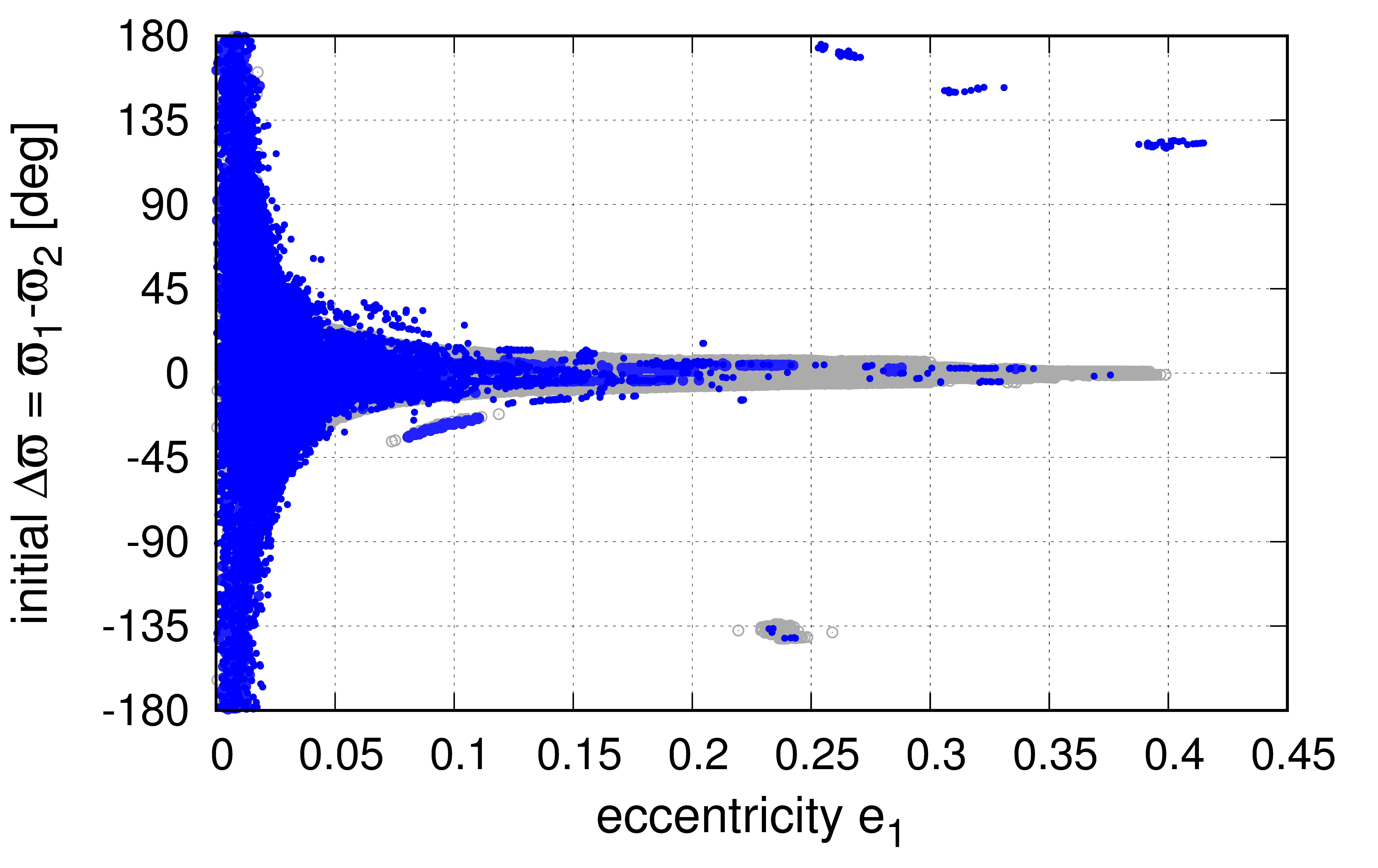
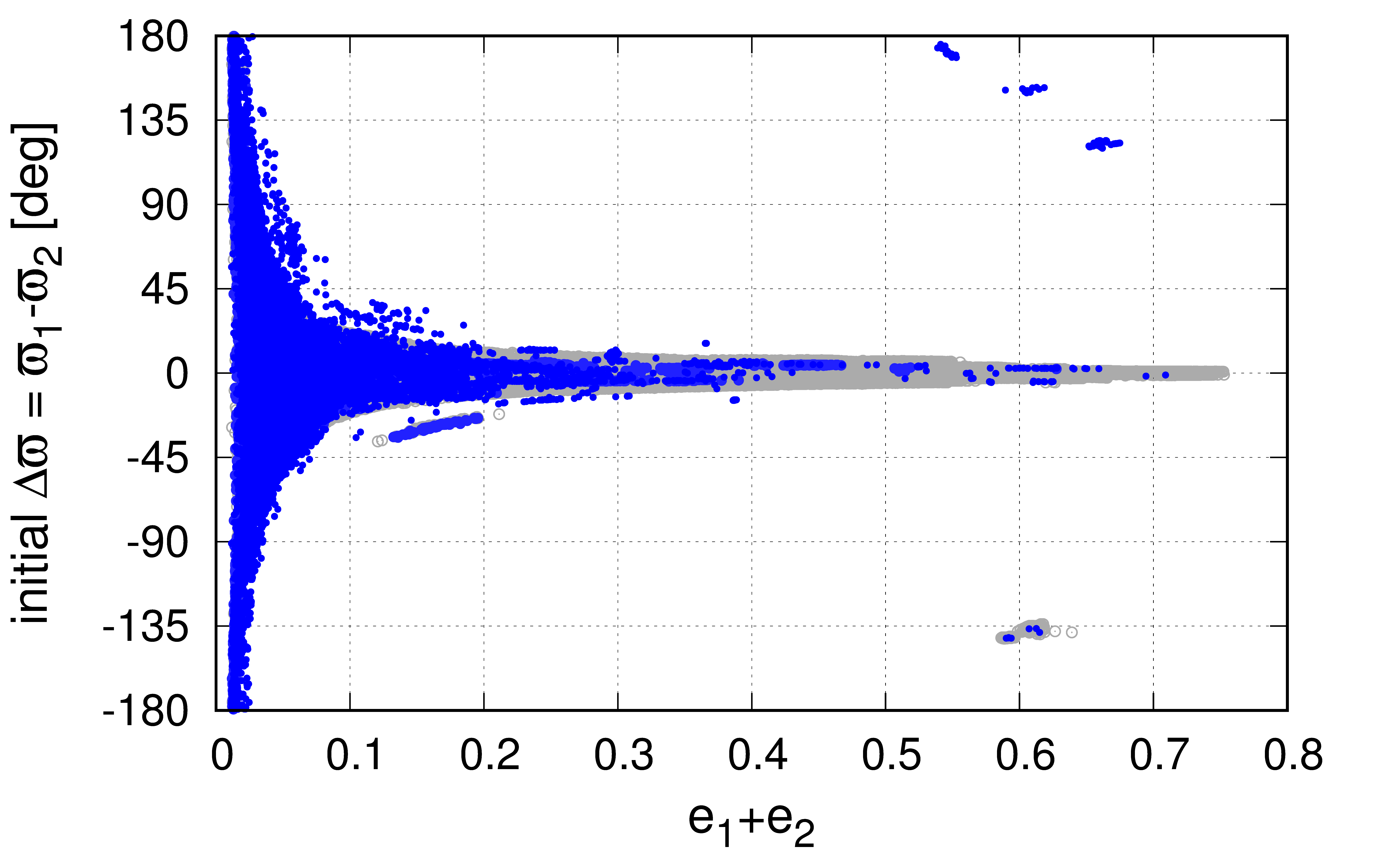
We first performed an extensive search with the GEA, collecting sets of solutions in each multi-CPU run. We did not impose any prior information on the model parameters in this survey, however we should not expect that the problem of unconstrained eccentricities could be avoided. Indeed, we found a continuum of models with d, well determined orbital periods and transit epochs , . The error floor days is roughly uniform for all these solutions. The -parameters transformed to the -elements () form a pin-like structure in the - and -planes, as shown in Fig. 1. The two panels look similar, because (see below). When the eccentricities reach moderate values up to , the TTV models are found close to –axis. A similar effect has been observed for other Kepler systems (Jontof-Hutter et al., 2016). It is not clear whether the apsidal alignment could be physical in the presence of planetary migration. As shown in (Xiang-Gruess & Papaloizou, 2015) aligned configurations for second order MMRs can be formed through migration, however that happens for the eccentricities significantly different one from another, not for like for Kepler-29. Aligned configurations studied in the cited paper remind systems in 2:1 MMR that move, during the migration, along a branch of stable periodic configuration and eventually change the libration centre of from to (e.g., Ferraz-Mello et al., 2003). When much more likely, and naturally emerging are resonant configurations with anti-aligned apsides, which are also present in Fig. 1 for small eccentricities.
Figure 1 illustrates also the results of the stability analysis for the models gathered. Due to relatively large masses of Earth masses, and close orbits, significant mutual perturbations could be possible. Therefore, for all solutions with we computed their MEGNO signatures for 64 kyrs ( outermost orbits). Such an interval well covers the characteristic short-term dynamical time-scale associated with the 9:7 MMR. In the case of the Kepler-29, dynamically stable models may be found in similarly wide range of the parameter plane. Curiously, stable solutions that fit the TTV data exist for as large as 0.3-0.4. Besides the pin-like structure, we also found isolated islands of high-eccentricity solutions beyond the axis. These models could be rather associated with librating around .
planet Kepler-29 b Kepler-29 c 5.7 4.9 [d] 10.33585 13.29292 0.0046 0.062 -0.009 0.05 0.0154 0.062 0.008 0.05 [d] 72.4200 0.0041 65.1830 0.0048 0.0928613 0.1098205 0.0160 0.01169 [deg] 73.44 139.94 [deg] -96.18 96.99 [d] 0.009 0.001 [d] 0.0145
Therefore, even if the stability constraints are considered, we actually cannot choose a “proper” or “best-fitting” configuration of the system. More tight constraints are required. At the first step, such constraints may be imposed by a statistical eccentricity distribution expected for compact Kepler systems.
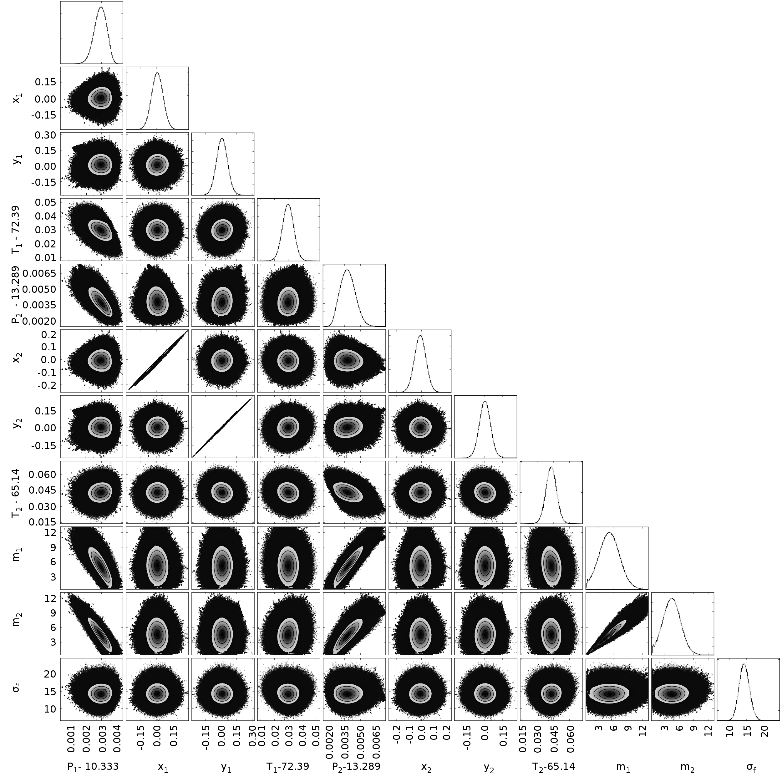
We preformed MCMC experiments to account for the physical limits of elements. The results are illustrated in Fig. 2. It shows one– and two–dimensional projections of the posterior probability distribution for Gaussian prior set to with zero mean and the variance equal to 0.1. Computations were performed in multi-CPU environment, making it possible to evaluate as much as 1,024,000 iterations to avoid the auto-correlation effect. Each run composed of 256 emcee “walkers” initiated in a small ball around low- solutions found in the GEA search. The posterior is uni-modal and centred close to with masses and for the inner and outer planet, respectively. The posterior distribution does not change its character, i.e., relatively well determined peaks when the -prior has the variance set to 0.05, 0.1, 0.25 and 0.33, yet the masses are strongly correlated. If the -priors are uniform, masses and -elements are not constrained.
For all Gaussian priors, we found strong linear correlations between pairs of and . These linear correlations could mean a tight alignment of apsidal lines which is a common dynamical feature of the low-order MMRs. This is likely a general effect discussed by Jontof-Hutter et al. (2016) for the first order MMRs. It may be explained by the evolution of eccentricity vectors , which are not constrained individually, but their components are tightly correlated.
The orbital period ratio in the best-fitting solutions is very close to 9/7, indicating a possible MMR. We searched for signatures of the 9:7 MMR by computing amplitudes of the critical angles of solutions sampled in the MCMC experiments. When a candidate solution showed d, we numerically integrated the -body equations of motion, and the full amplitudes of all critical angles have been determined for yrs (. The amplitudes are expressed through
where is for any of the three critical arguments of the 9:7 MMR, , (Eq. 2).
The results are illustrated in Fig. 3 for three planes of orbital parameters selected from samples with d (grey dots). The grey area is filled, as guaranteed by the MCMC sampling, hence we may be confident that the search covers all the relevant parameter space. Solutions with (i.e., with full amplitude of or ) are marked with blue filled circles. This experiment shows that solutions with anti-aligned apsides are preferred for small eccentricities , while models with librating critical angles and aligned apsides are found mostly for moderate and large eccentricities.
Curiously, the distribution of models in the ()–plane forms a strip having a sharp “cut-off” at small eccentricities region (). This effect could be explained by measurable, mutual interactions of the planets. Since the total angular momentum must be conserved, it implies eccentricities variations in anti-phase.
2.2 The resonant character of the system
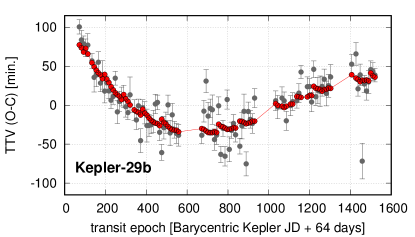
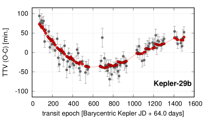
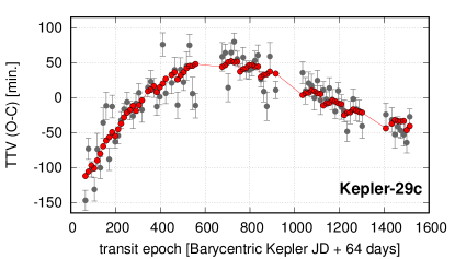
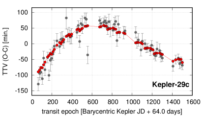
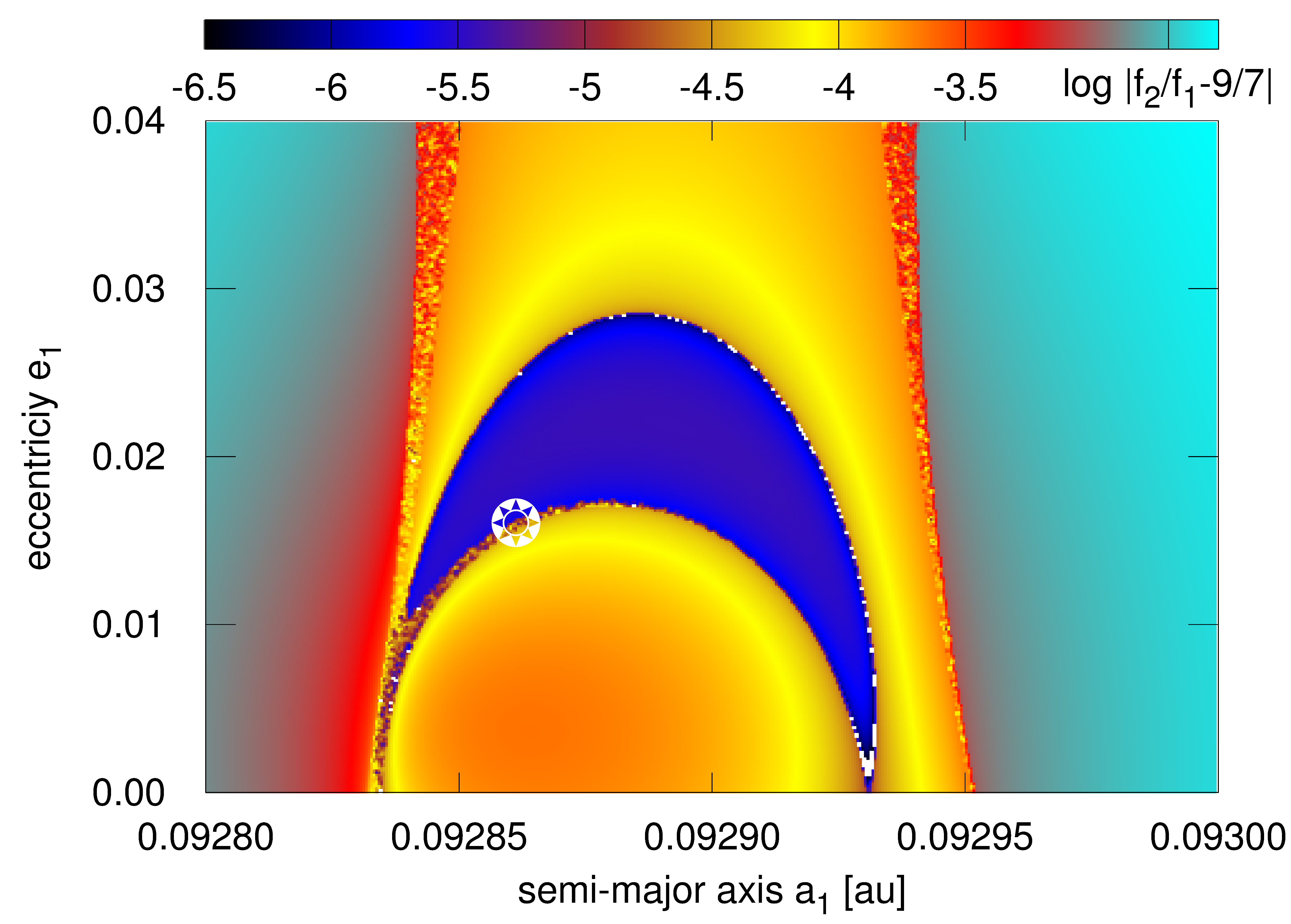
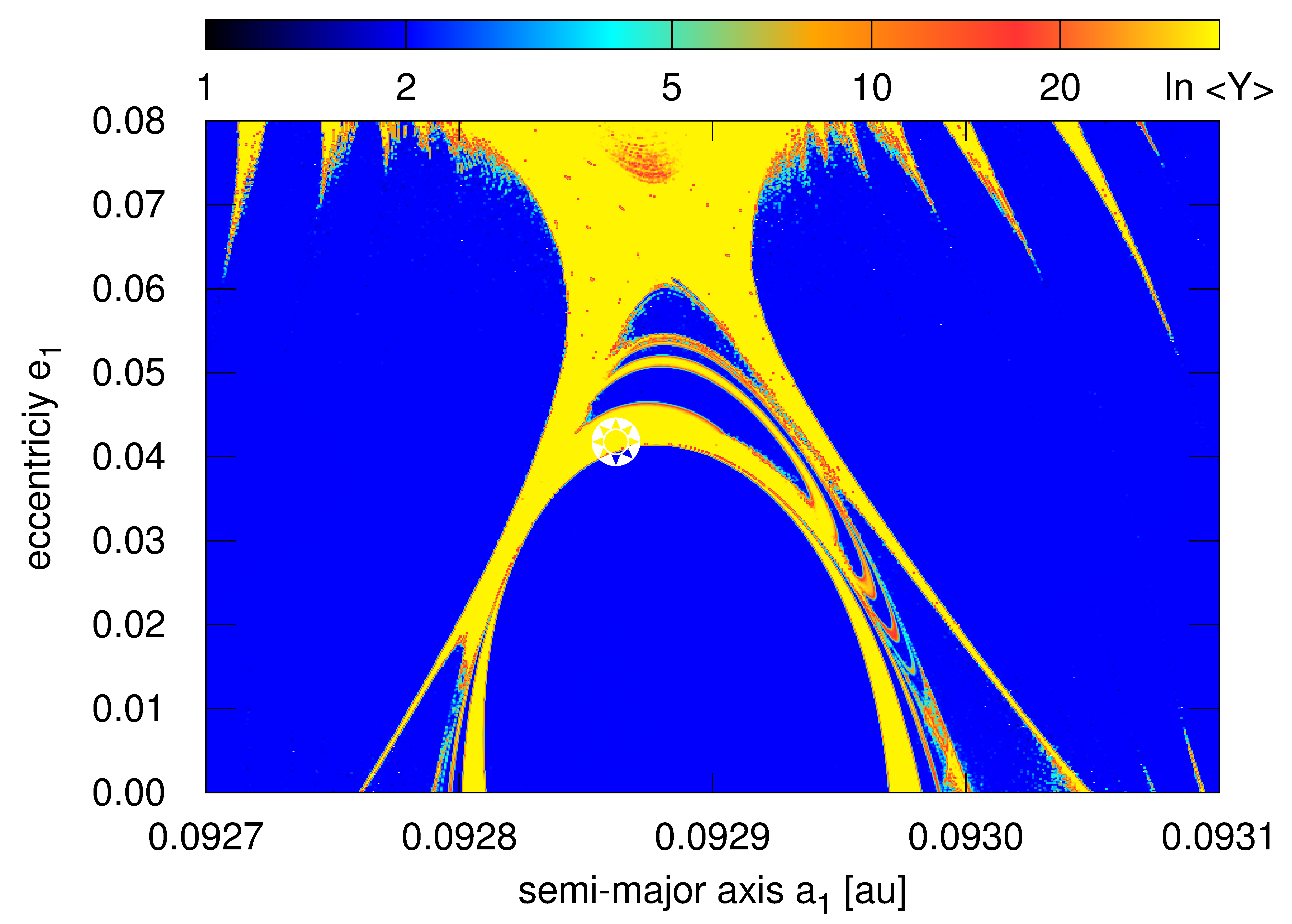
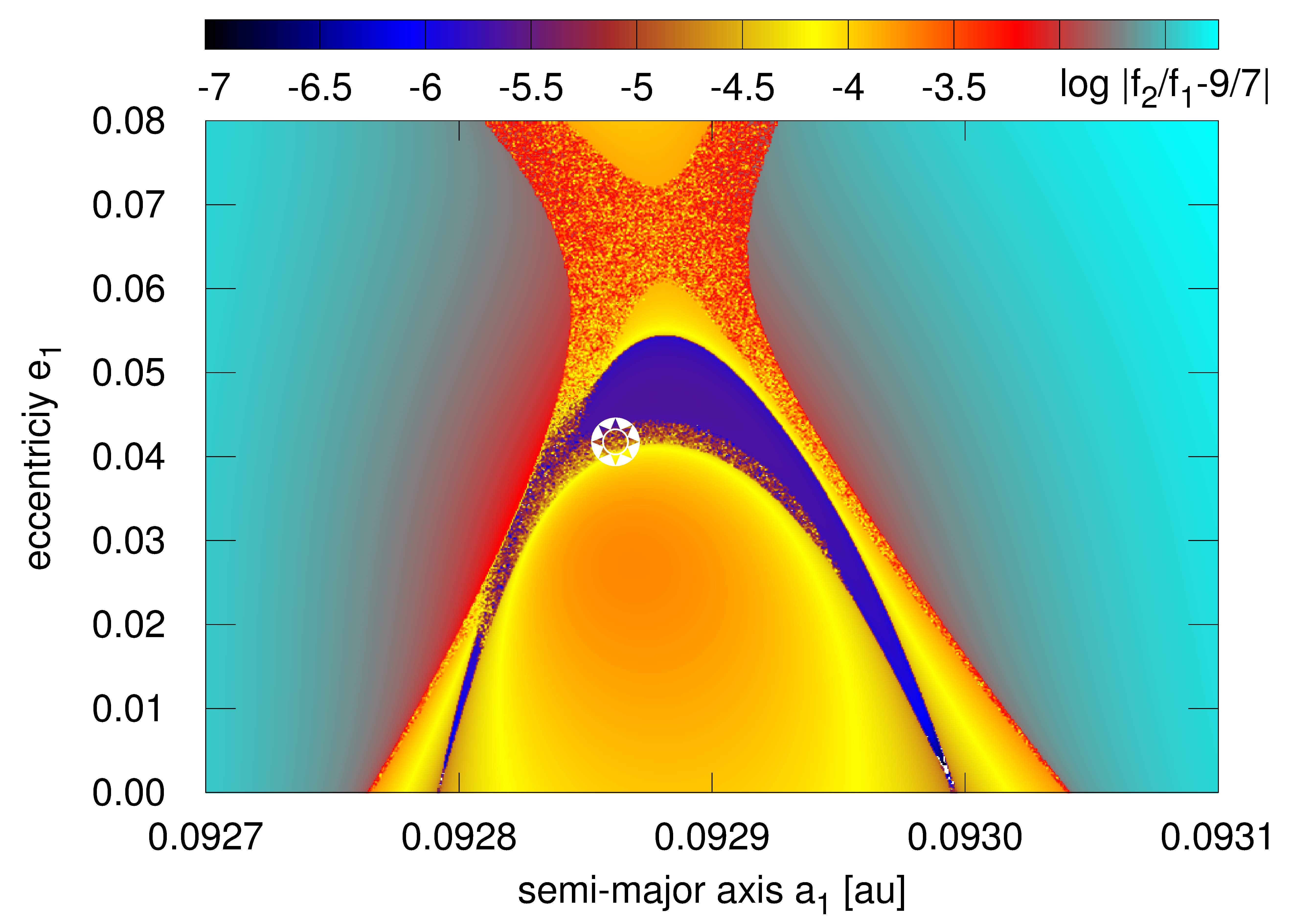
We computed 2-dim dynamical maps in the neighbourhood of two representative best-fitting solutions to visualise the dynamical structure of the 9:7 MMR. First of these solutions is the result of the MCMC sampling for the variance of set to . Its parameters are given in Tab. 1 and the synthetic TTV signals are presented in Fig. 4. The top-row of Fig. 5 shows dynamical maps in the –plane for this model. All other orbital elements are kept at their best-fitting values. For each initial condition at the grid, the -body equations of motion where integrated up to kyr. This corresponds to , sufficient to detect short-term chaotic motions for the MMRs instability time-scale (e.g. Goździewski & Migaszewski, 2014). As the dynamical maps show, the observational uncertainties of and are much smaller than the width of the 9:7 MMR, see Fig. 5. The best-fitting solution is found, somehow ironically, just in a narrow unstable structure which may be identified with the separatrix. The 9:7 MMR structure may be even better visible in the right-hand panel of Fig. 5 which is for the frequency map of the system and shows deviations of the ratio of mean motions (fundamental frequencies) from the exact 9/7 value. The 9:7 MMR spans the middle part of the map, depicted as wide grey/yellow strip of regular motions limited by vertical separatrices. In the middle of this strip, a boomerang-like structure appears with deviations from the 9/7 ratio as small as and sharp borders coinciding with curved, narrow separatrices identified in the MEGNO map.
We found that the critical angles are not fully adequate signatures of the 9:7 MMR since they may librate with large full amplitudes reaching , even in the boomerang-like region characterised with almost exact 9/7 ratio of the orbital periods.
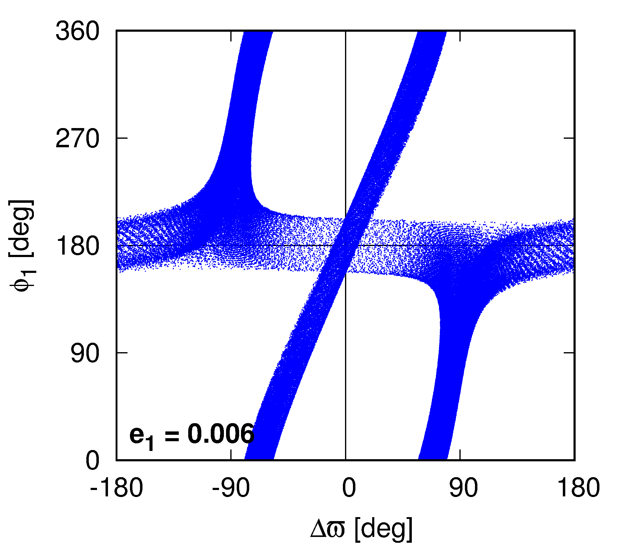
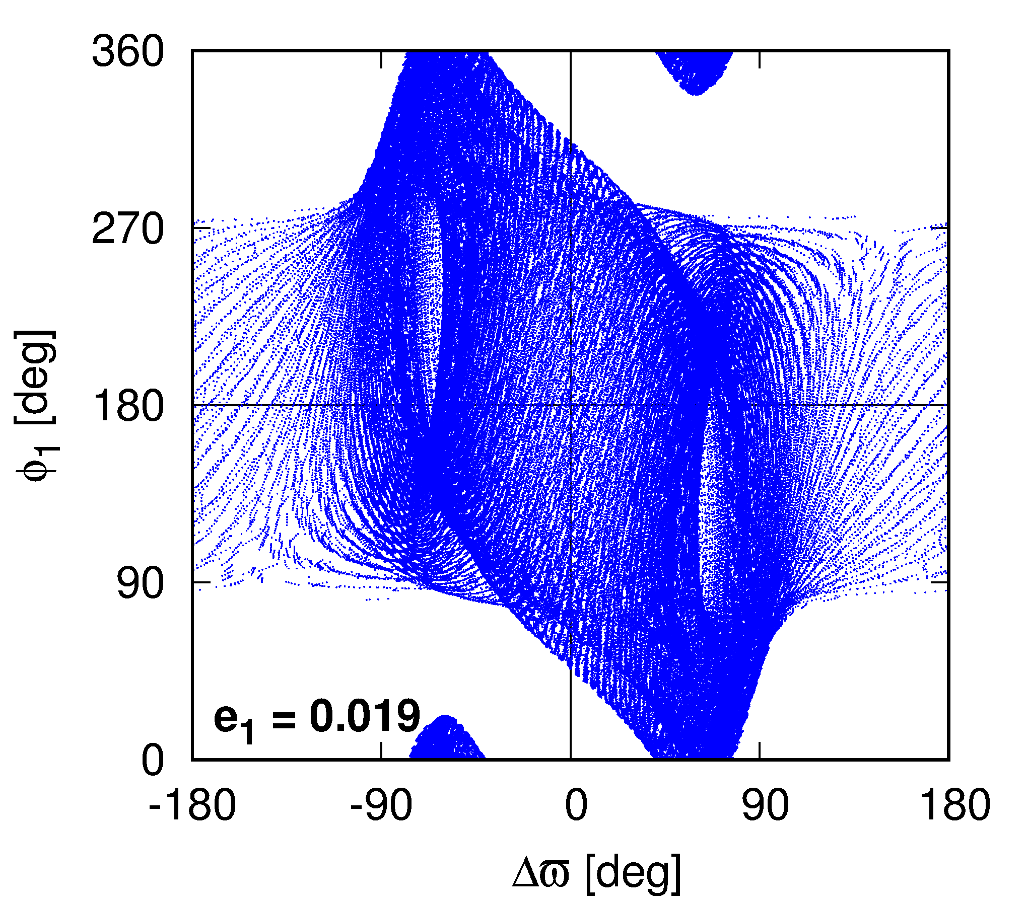
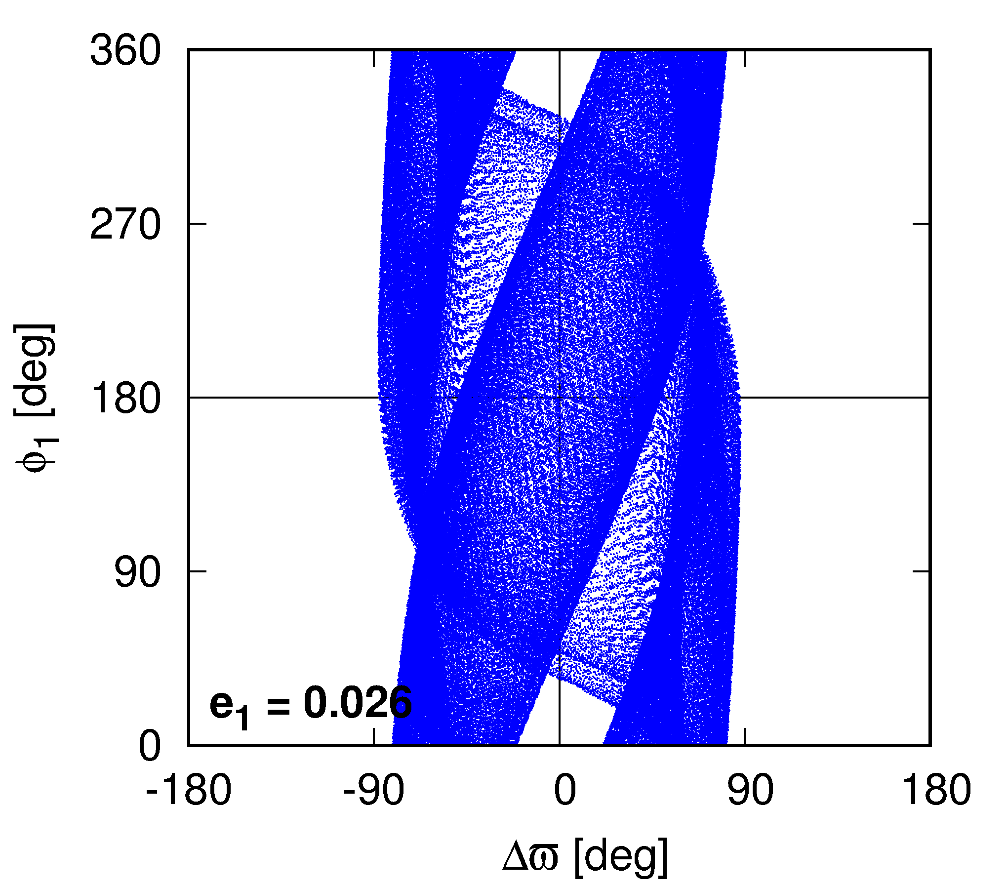
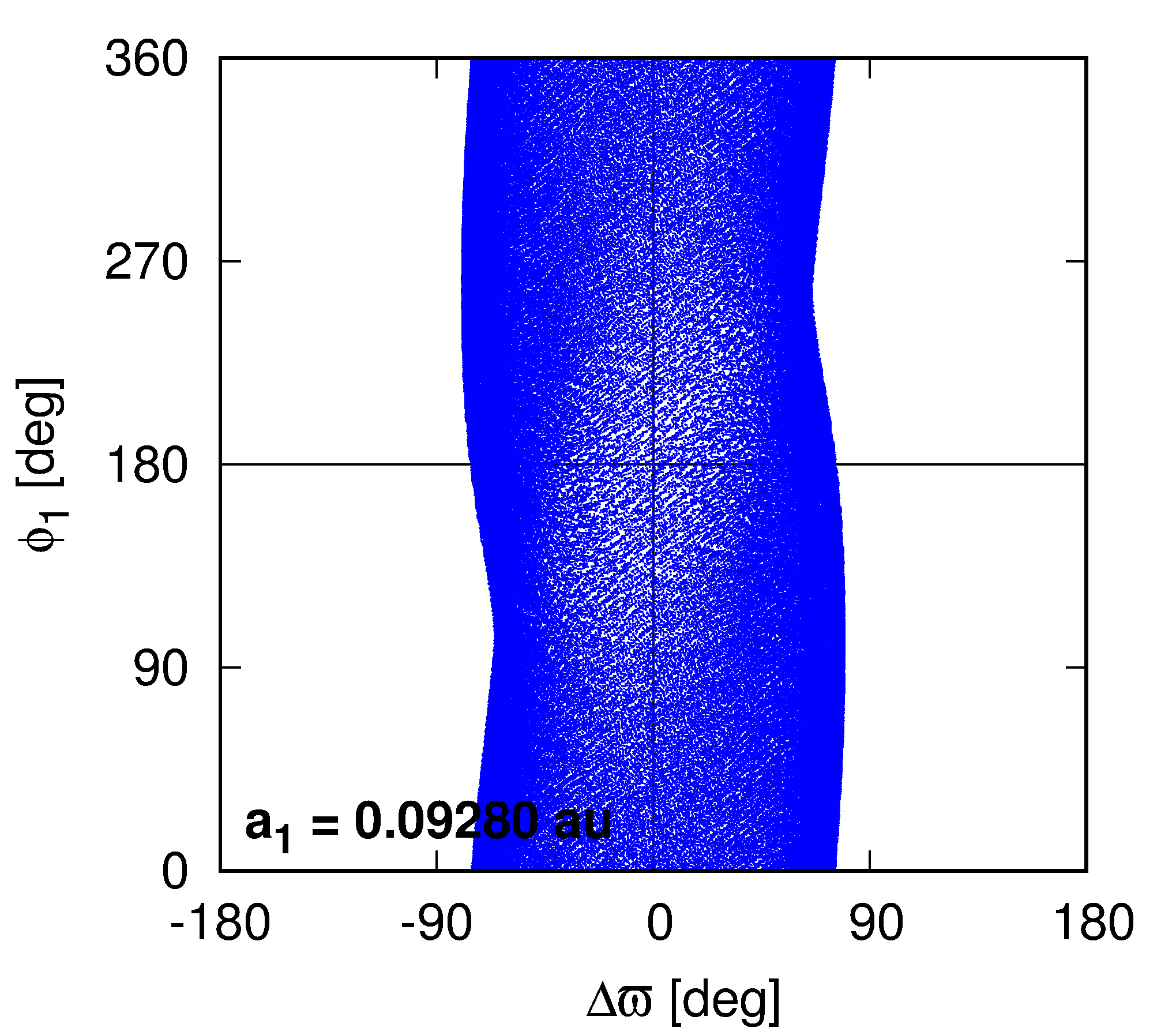
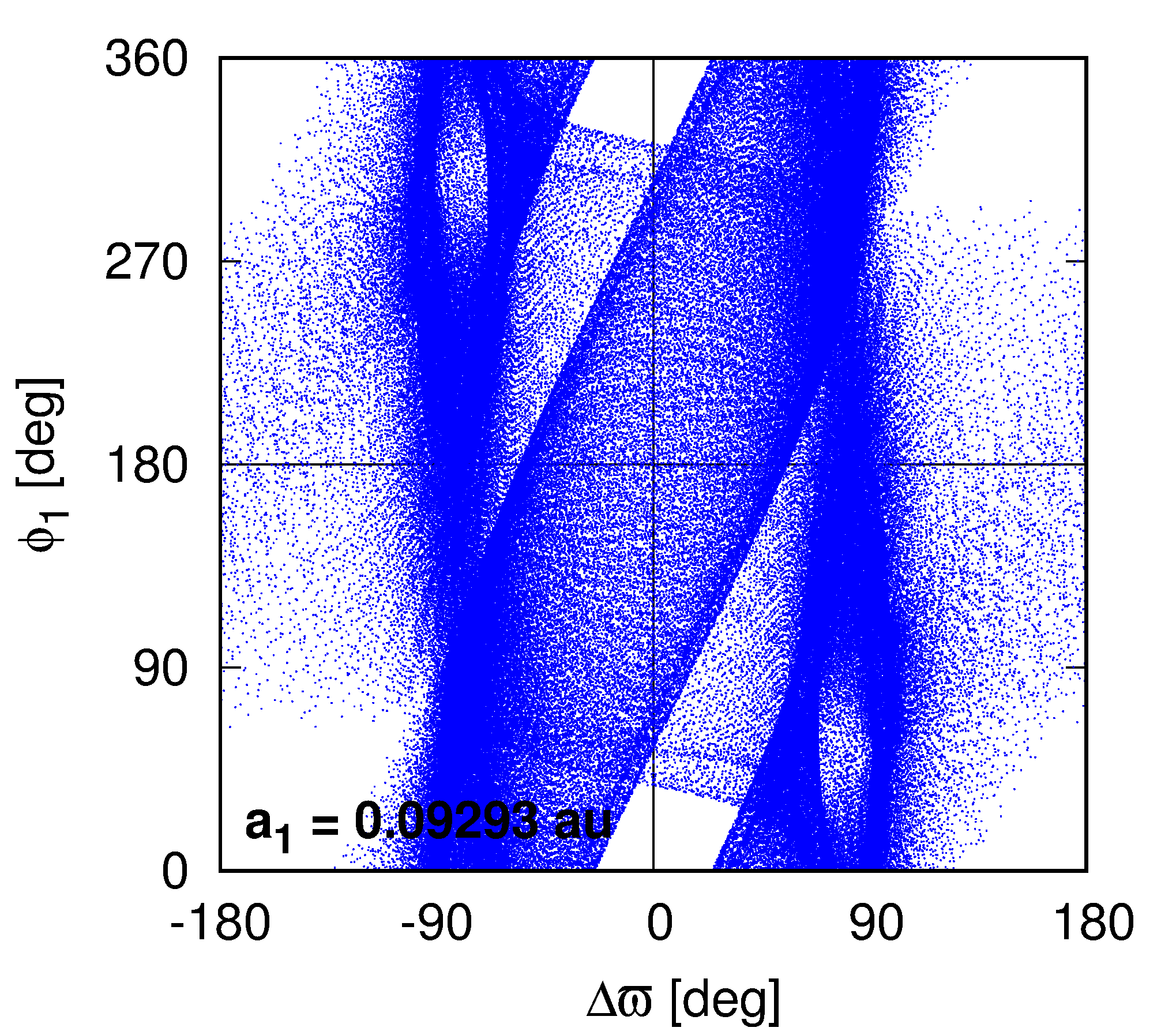
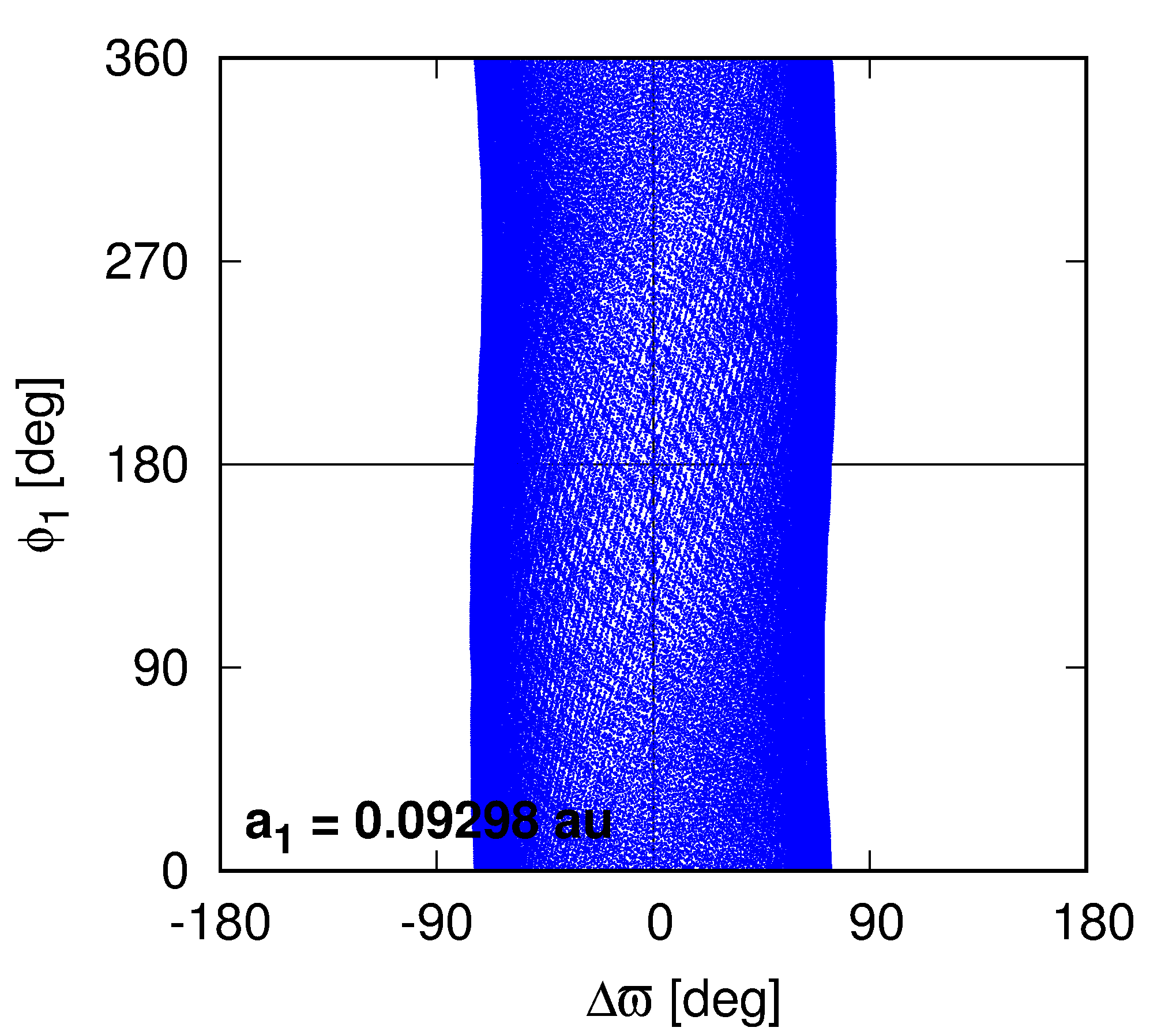
Yet a highly ordered evolution of during first 36 kyr ( outermost periods) is illustrated in the top row of Fig. 6 for three initial conditions selected at maps in Fig. 5, with the same elements as the best-fitting model, besides changed . The left-hand panel is for (below the lower separatrix of the boomerang-like structure), (close to the nominal solution, between the separatrices), and (above the upper separatrix). In all these cases a clear, resonant behaviour of the system is apparent which we understand here as a strong correlation of the critical angles rather than low-amplitude librations of these critical arguments. The primary indication of the presence of the resonance are the dynamical maps, Fig. 5 and the particular, vertical structure, which is common for MMRs in the -plane.
There is also a clear difference between evolution of the critical angles inside and outside the 9:7 MMR structure. To show this, we integrated two configurations with and (the left and the right-hand panels of the bottom row of Fig. 6, respectively) that are located outside the resonance. In contrast to highly correlated behaviour of the angles inside the vertical structure, illustrated in the top row of Fig. 6, in both these cases the evolution of the angles is not ordered in the sense explained above. Angle can be equal to or when equals . The middle panel in the bottom row illustrates the resonant behaviour, however the initial , so the system is very close to the separatrix between resonant and non-resonant regions. Although the system evolves almost in a whole -plane, similarly to the top row of Fig. 6, the angles are synchronised and when or , cannot be .
We also found clear semi-major axes oscillations, expected for systems in MMR, whose amplitude is a few times larger in the MMR region, when compared to solutions beyond the MMR structure (not shown here). Moreover, the curved, thin chaotic borders encompassing the boomerang-like structure inside the MMR could be identified with separatrices of secondary resonances of the frequency of oscillation of the semi-major axes (the resonant frequency) with the frequency of librations of the secular angle (Morbidelli & Moons, 1993; Michtchenko & Ferraz-Mello, 2001).
The bottom row in Fig. 5 is for the dynamical maps computed for MCMC derived models with the eccentricity priors set to . This prior leads to systematically larger osculating eccentricities, however the respective posterior distributions looks similarly as in Fig. 2. Curiously, the best-fitting solution remains “glued” to the unstable separatrix of the boomerang-like structure.
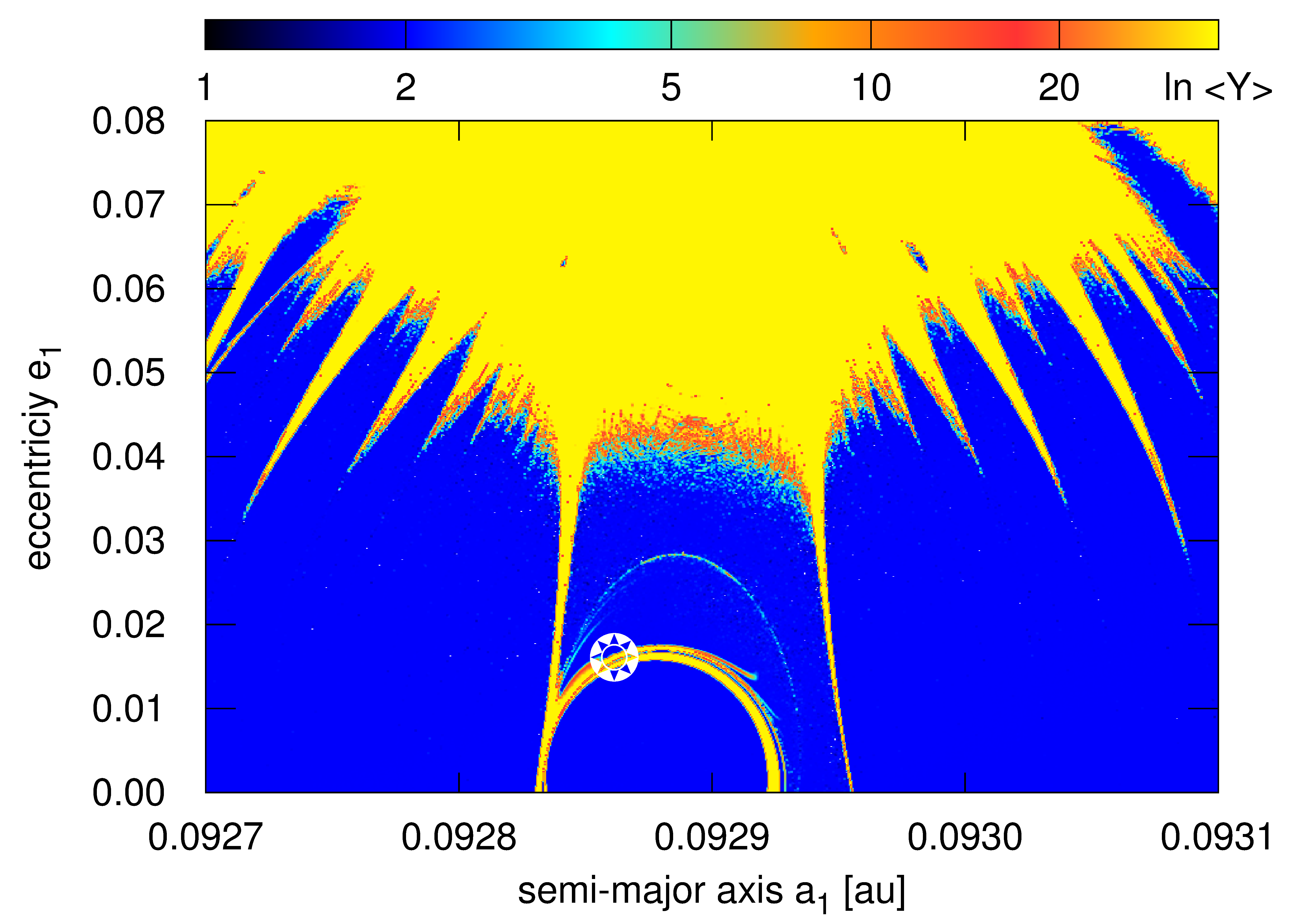
A problem of constraining the dynamical model of Kepler-29 is finally illustrated in Fig. 7 which shows a MEGNO map for osculating elements from a small island of stable solutions around ), see Fig. 1. Each point in this map has been integrated for 64 kyrs, which guarantees the Lagrange stability for 10-100 times longer interval, hence for Myrs. The tested initial condition is found in an island in a kind of archipelago with eccentricities as large as . Figure 1 displays a few isolated models of this type with large eccentricities.
3 Periodic orbits
In the previous sections we could not determine any unique model of the Kepler-29 system with both the observational and dynamical constraints. Therefore we aim to impose additional constraints through the most likely convergent planetary migration of the system in the past. As it has been shown (Beaugé et al., 2003, 2006; Hadjidemetriou, 2006; Migaszewski, 2015), systems of two planets that undergo convergent migration evolve along families of periodic orbits. Although the cited papers are devoted to first order MMRs, one could expect that also for a second order MMR, like 9:7, periodic orbits play an important role. Therefore we seek for families of periodic orbits of 9:7 MMR and show where the configurations that fit the TTV data locate with respect to them.
![[Uncaptioned image]](/html/1609.09135/assets/fig3a.png)
![[Uncaptioned image]](/html/1609.09135/assets/fig3b.png)
![[Uncaptioned image]](/html/1609.09135/assets/fig3c.png)
3.1 The representative plane of initial conditions
In order to address those issues, we apply the so called representative (symmetric) plane of initial conditions (e.g., Beaugé & Michtchenko, 2003) which makes it possible to illustrate global, qualitative features of the multi-dimensional and multi-parameter planetary systems.
Before introducing the -plane, we recall some essential facts about resonant configurations of two planets in coplanar orbits. Their dynamics may be reduced through the averaging over the fast angles to a two-degree-of-freedom Hamiltonian. This Hamiltonian possesses two first integrals, i.e., the total angular momentum and the so called spacing parameter where , , and , (Michtchenko & Ferraz-Mello, 2001; Beaugé & Michtchenko, 2003).
The averaged Hamiltonian can be expressed through where the canonical variables are and with . It can be shown that for critical values of . Therefore the equilibria of the averaged system, that are periodic configurations of the full three-body problem, do exist for these four pairs of angles. (Note that changing signs for both the angles simultaneously does not lead to any change in the Hamiltonian.) Such configurations are called apsidal corotation resonances (ACR). Here we consider symmetric ACR only.
The canonical averaging can be done numerically or analytically. The explicit form of the averaged Hamiltonian is
where the disturbing function reads as follows:
| (3) |
This integral can be evaluated numerically (Michtchenko et al., 2006) or analytically. For this operation the function under the integral must be expanded in power series w.r.t. the small parameters, like eccentricities or semi-major axes ratio, (e.g., Beaugé & Michtchenko, 2003). Here, is a sum of the secular and resonant terms, following a recipe in (Murray & Dermott, 1999). We selected terms up to the fourth power in the eccentricities, which provides a very good approximation for eccentricities , and with no terms related to the inclinations and nodal longitudes, since we assume a coplanar configuration. The explicit form of the averaged Hamiltonian is given in Appendix A.
The representative (or characteristic) plane of initial conditions is a plane of eccentricities. A point in this plane determines semi-major axes through the first integrals and . The initial condition of a given system contains also angles and chosen from the critical set of . Each orbital configuration with angles that circulate or librate around pairs of critical values given above must intersect this plane (Michtchenko & Ferraz-Mello, 2001). Therefore, in order to study the dynamics of such systems globally, it is sufficient to consider the four sets of initial resonant angles in the -plane. However, the –plane defined in this way is representative only for symmetric configurations, for which equals or . There could, in principle, also exist asymmetric configurations with different libration centres (Beaugé et al., 2003). Since the majority of the best-fitting configurations of the Kepler-29 system are symmetric (apart from, possibly, a few islands with large eccentricities, Fig.1), we limit our analysis to the symmetric configurations only.
Furthermore, instead of we choose their combinations, the secular angle and one of the critical arguments of the 9:7 MMR, , which are more convenient for an interpretation of their evolution. The representative angles at the -plane are then and , and the -plane coordinates can be defined as , where both cosines are equal to or to .
Although the -plane has been defined for the averaged Hamiltonian with two degrees of freedom, we can use the same concept also for the full three-body, non-averaged system. It is convenient to show orbital models that fit the observations w.r.t. the periodic orbits represented as equilibria of the averaged system.
3.2 TTV-constrained models in the -plane
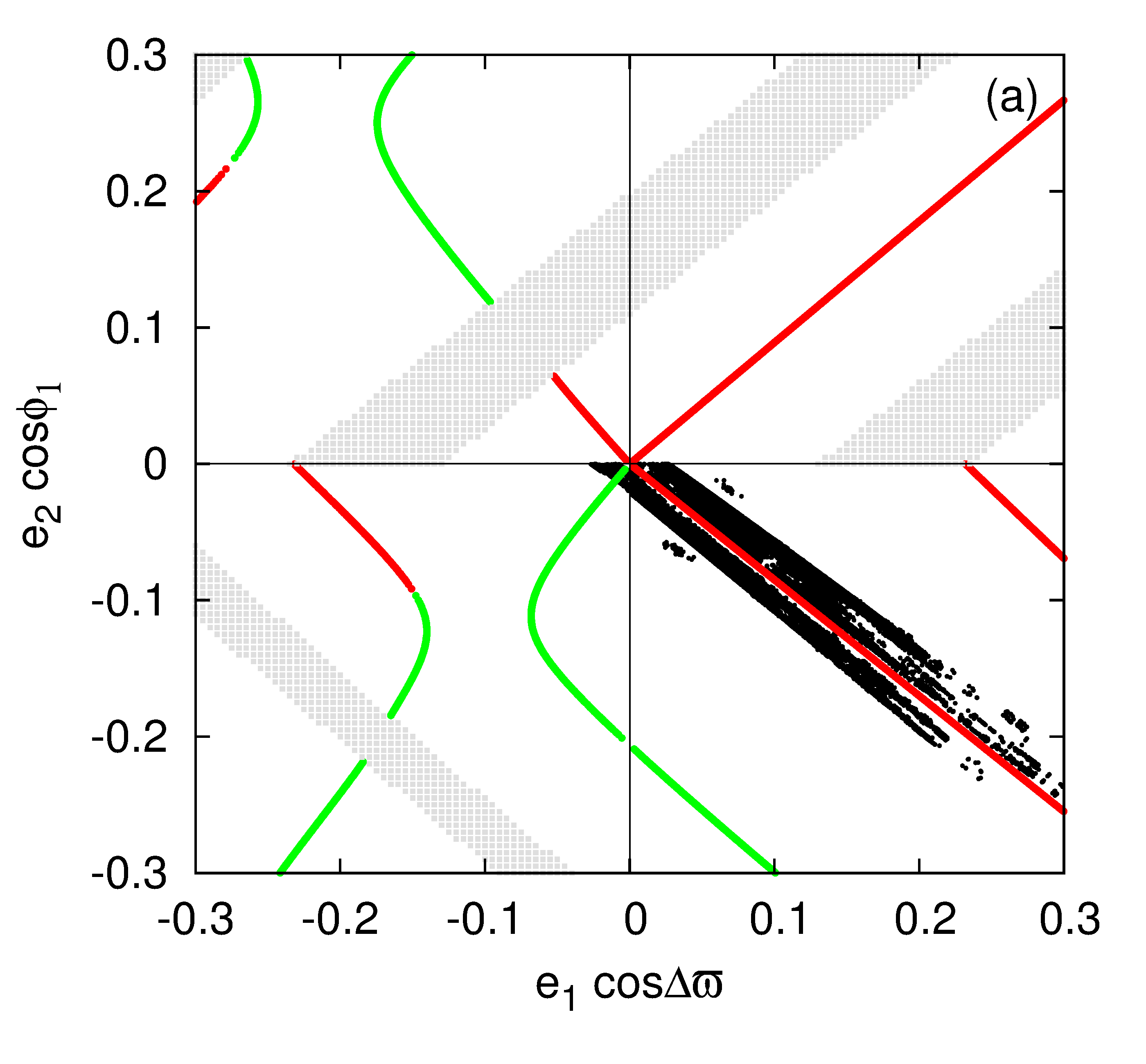
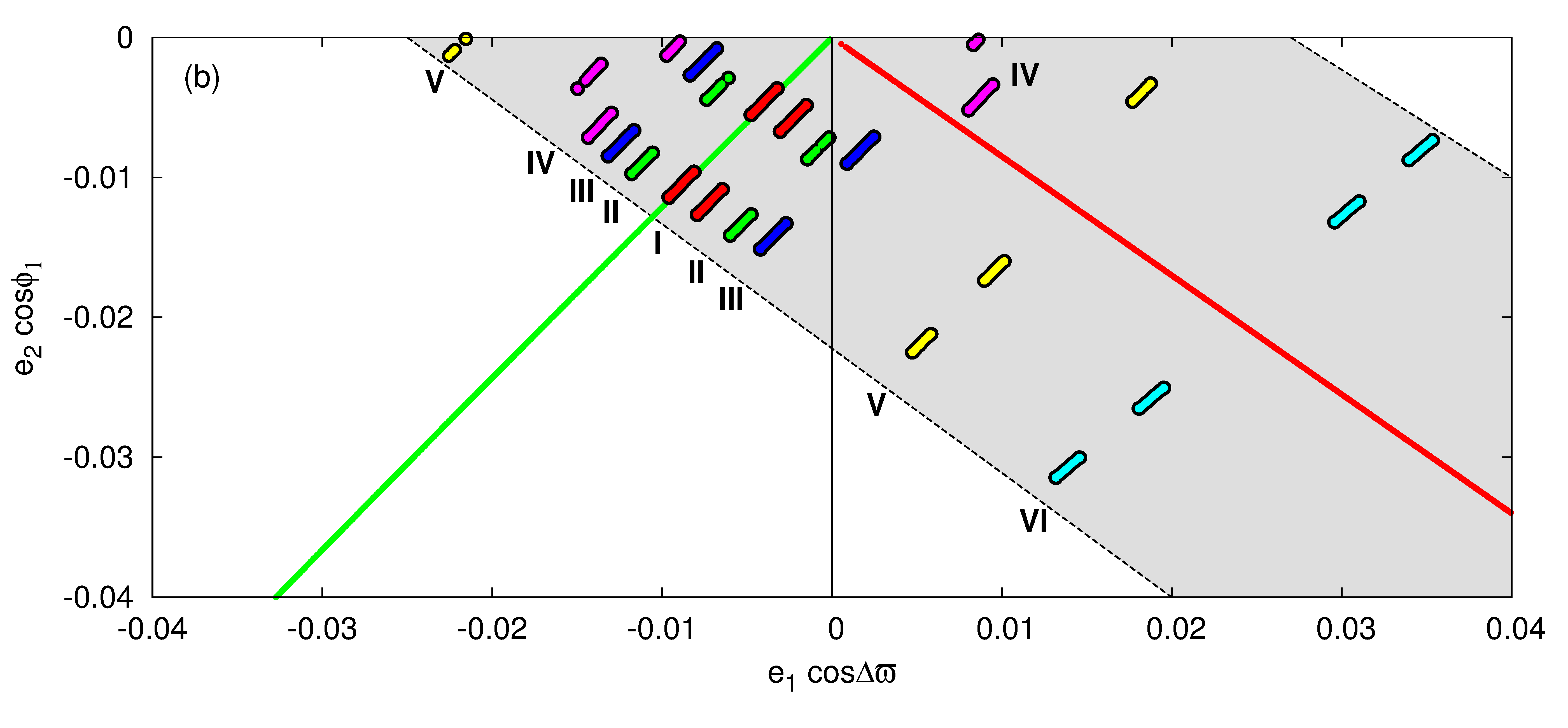
We narrowed the set of dynamically stable initial conditions, as illustrated in Fig. 3, by days. To map this set on the -plane, we integrated the -body equations of motion forward for . Each time when (expressed in radians; for numerical reasons of limited integration time, we chose a small limit of for the intersection of the -plane), osculating elements were transformed to coordinates at the -plane and presented in the left-hand panel of Fig. 8. Usually, each initial configuration evolving in time results in more than one point at this plane. For the reduced system with two degrees of freedom one obtains: i) one point at the -plane if the system is in a stable equilibrium; ii) two points if it is a stable periodic configuration of the reduced system (fixed point at the Poincaré cross section); iii) four points if the reduced system evolves along quasi-periodic orbit; iv) a continuum of points for chaotic evolution. The full (non-averaged) system intersects the plane in four groups of points if its reduced counterpart intersects the plane in four points.
As Fig. 8 shows, stable models that fit the TTV data form a strip at the -plane along a line originating from and directed towards higher eccentricities in the quarter of the plane with and . There are points in the –quarter as well, but no configurations intersect the upper half of the -plane ().
The second critical component of Fig. 8 is a representation of families of the periodic orbits. Green and red solid curves show families of stable and unstable equilibria of the reduced system (periodic configurations of the full system), respectively. The periodic system returns to its initial state after a certain period . For the periodic orbits in the 9:7 MMR it covers nine revolutions of the inner planet, and seven revolutions of the outer planet. Then the planets starting for instance from their pericenters will be back in the pericenters after the period . Also orbital elements will retain their initial values. Angles and will change, since the system precesses as a whole. For a given point we integrate the equations of motion and evaluate . We search for such (for a given ) that provides . In order to check the stability of a given periodic configuration we integrate the system for revolutions. A stable periodic configuration is preserved, while for unstable one, sooner or later the system evolves into different regions of the phase space.
Tracks of the periodic orbits in the -plane correspond to the equilibria of the averaged system. They may be found through solving the equations
since the partial derivatives over are zero at the whole -plane. The stability of equilibria of two-degree-of-freedom Hamiltonian systems can be verified through solving the eigenvalue problem for the linearised equations of motion. One can also check if a given point is an extremum of for fixed and . We verified that the branches of periodic orbits of the full -body equations of motion precisely coincide with the equilibria of the averaged system in the region of the -plane we will be interested in. This is valid for the averaging done analytically and numerically. However, the analytic averaging provides reliable results only for non-crossing orbits (crossing orbits are shown with grey dots in Fig. 8a). The numerically averaged Hamiltonian can be used to describe the dynamics even for crossing orbits, provided the perturbation to the Keplerian motions is sufficiently small.
Apparently, the best-fitting solutions appear along a family of unstable equilibria. We found this result somehow unexpected from the point of view of the formation of the system through the migration. Unstable periodic orbits in the proximity of the observationally constrained configurations may be also a factor provoking dynamical instability of the system. Although aligned configurations are, in general, not impossible to form within the migration formation scenario (e.g., Ferraz-Mello et al., 2003; Beaugé et al., 2003), the aligned configurations studied in the cited papers are related to the branch of stable equilibria. As shown in the previous Section, geometrical parameters of the system like eccentricities and pericenter longitudes are not well constrained due to low signal-to-noise ratio, narrow observational window and features of the TTV method. This permits us to look for solutions fulfilling also the migration constraints.
As (Migaszewski, 2015) has demonstrated, two-planet systems that undergo convergent migration end up in exact periodic configurations. Nevertheless, that conclusion referred to the first-order resonances and might not be fully applicable to the second-order MMRs. We will discuss this further in this paper. After inspecting the O-C diagrams of Kepler-29 system (see Fig. 4), one can conclude that it cannot be related to exactly periodic configurations. In such a case there would be no secular TTV signal of a period longer than the resonant period of days. However, such a signal of a few-year period is clearly visible in the data. Therefore, the real Kepler-29 cannot be a strictly periodic configuration. Nevertheless we show further that the migration is still very likely a way the system has been formed.
3.3 Particular solutions in the -plane
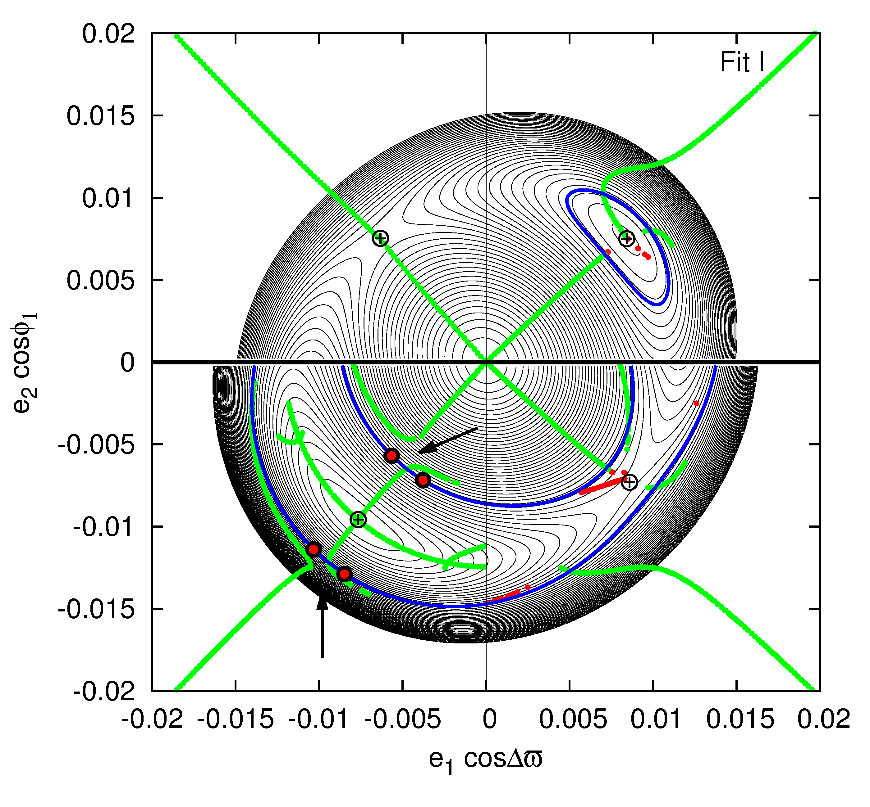
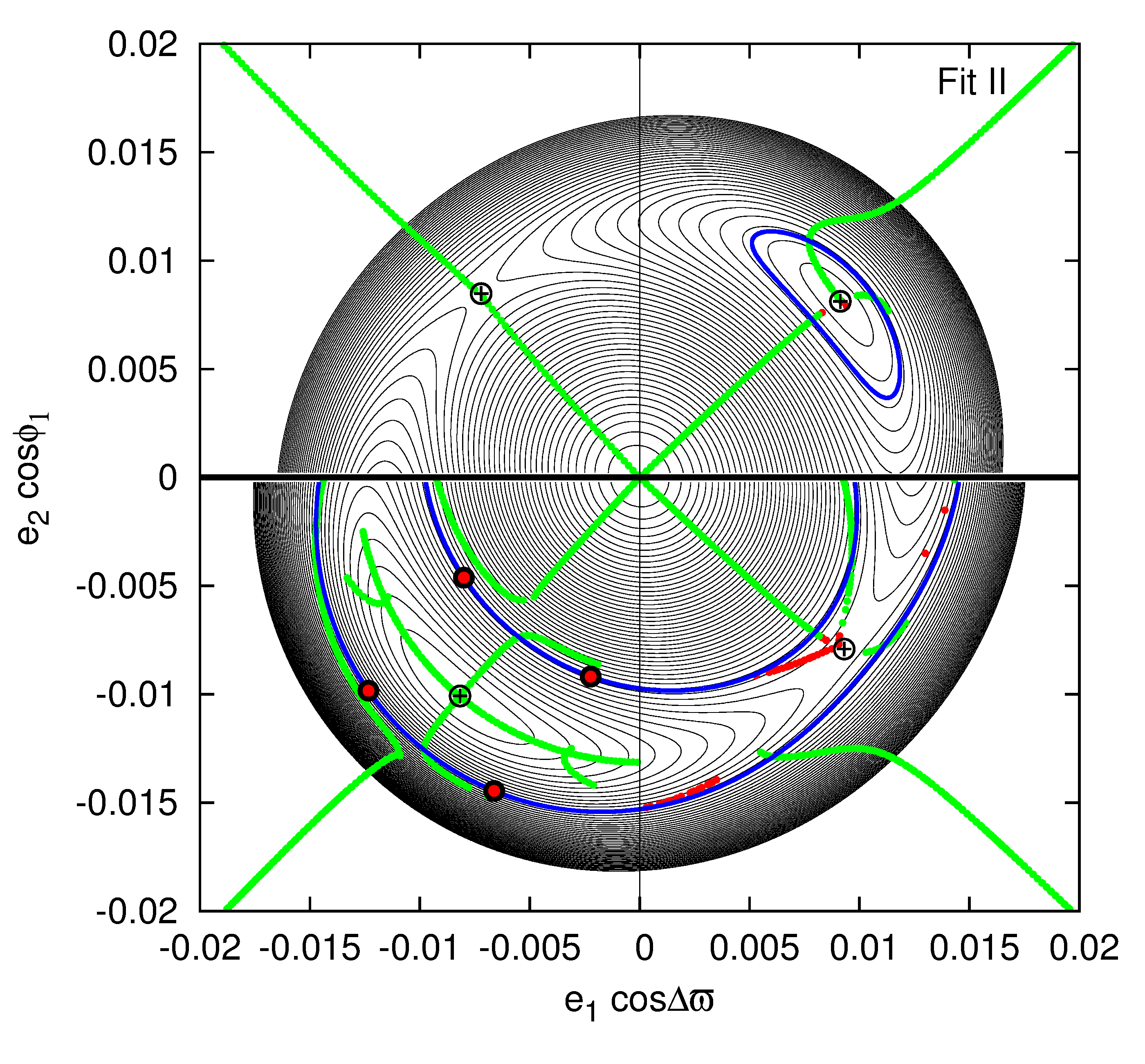
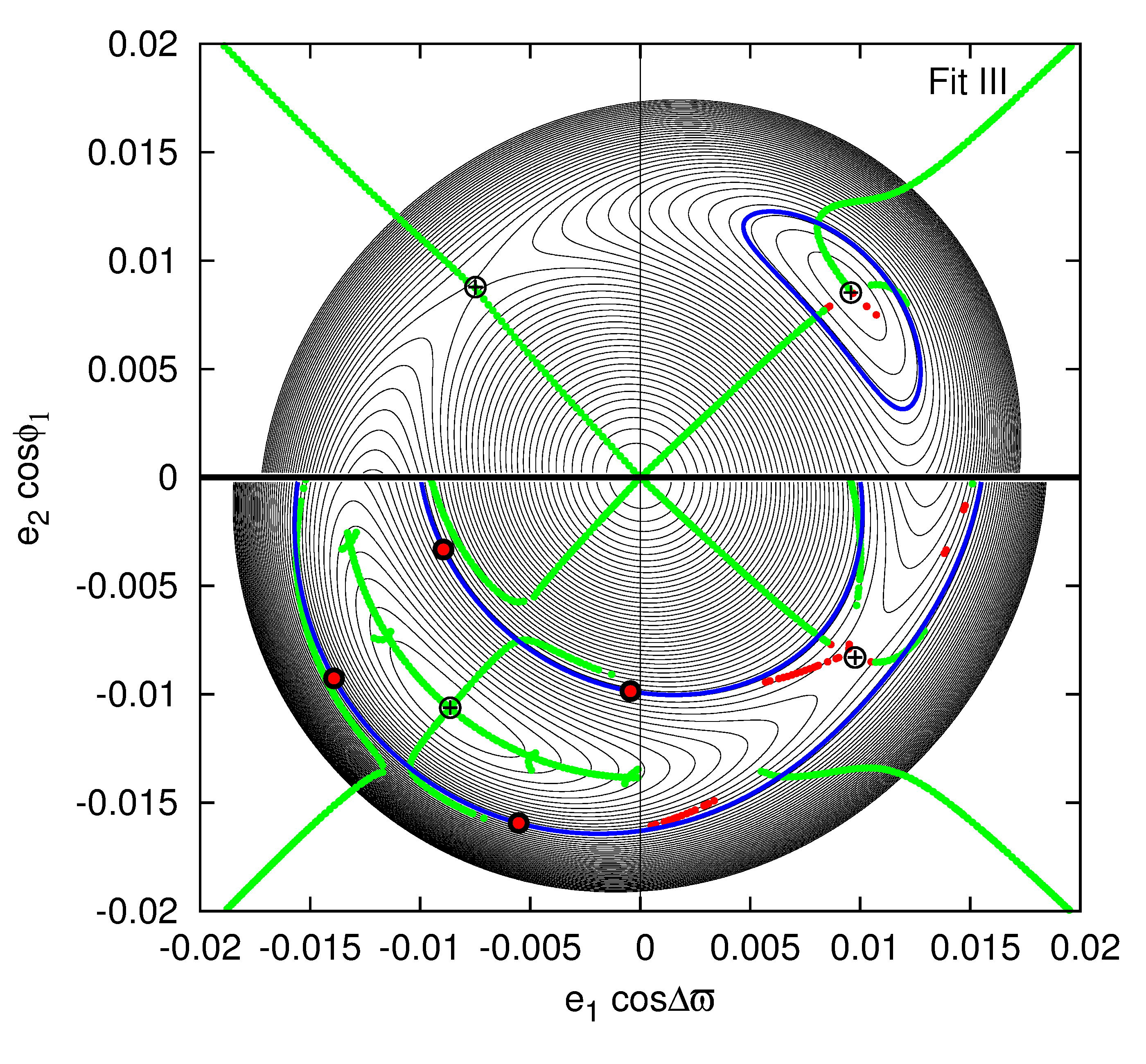
The right-hand panel of Fig. 8 illustrates models selected from the set of solutions that well reproduce the observations. Those six models (Tab. 2) were chosen as qualitative representatives for all the statistics of the best-fitting models. Model I (red points) intersects the -plane very close to the branch of stable equilibria and all four groups of points where the system intersects the –plane lie in the quarter. Model III (blue points) lies further from the stable branch than Model I, and its phase trajectory intersects both quarters with . Model II (green points) is an intermediate configuration between Models I and III. Its phase trajectory almost “touches” the quarter with . Model VI (cyan points) lies in vicinity of the unstable branch of equilibria in the quarter and intersects only this quarter. Models IV (magenta points) and V (yellow points) are intermediate states between Models III and VI. The sequence of models from I to VI shows a transition between configurations very close to the branch of stable equilibria and configurations close to the branch of unstable equilibria.
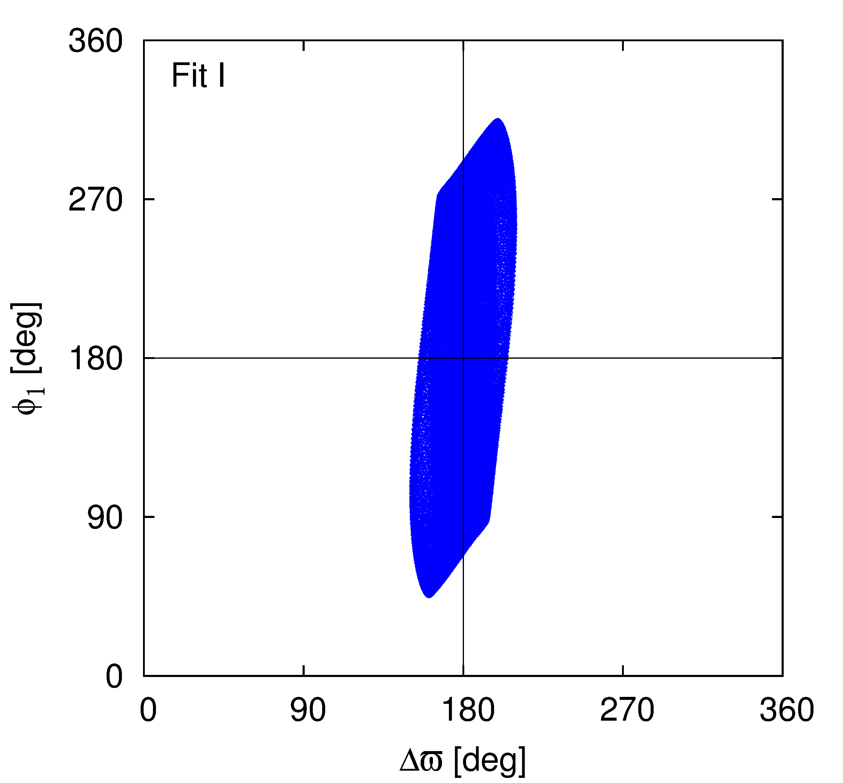
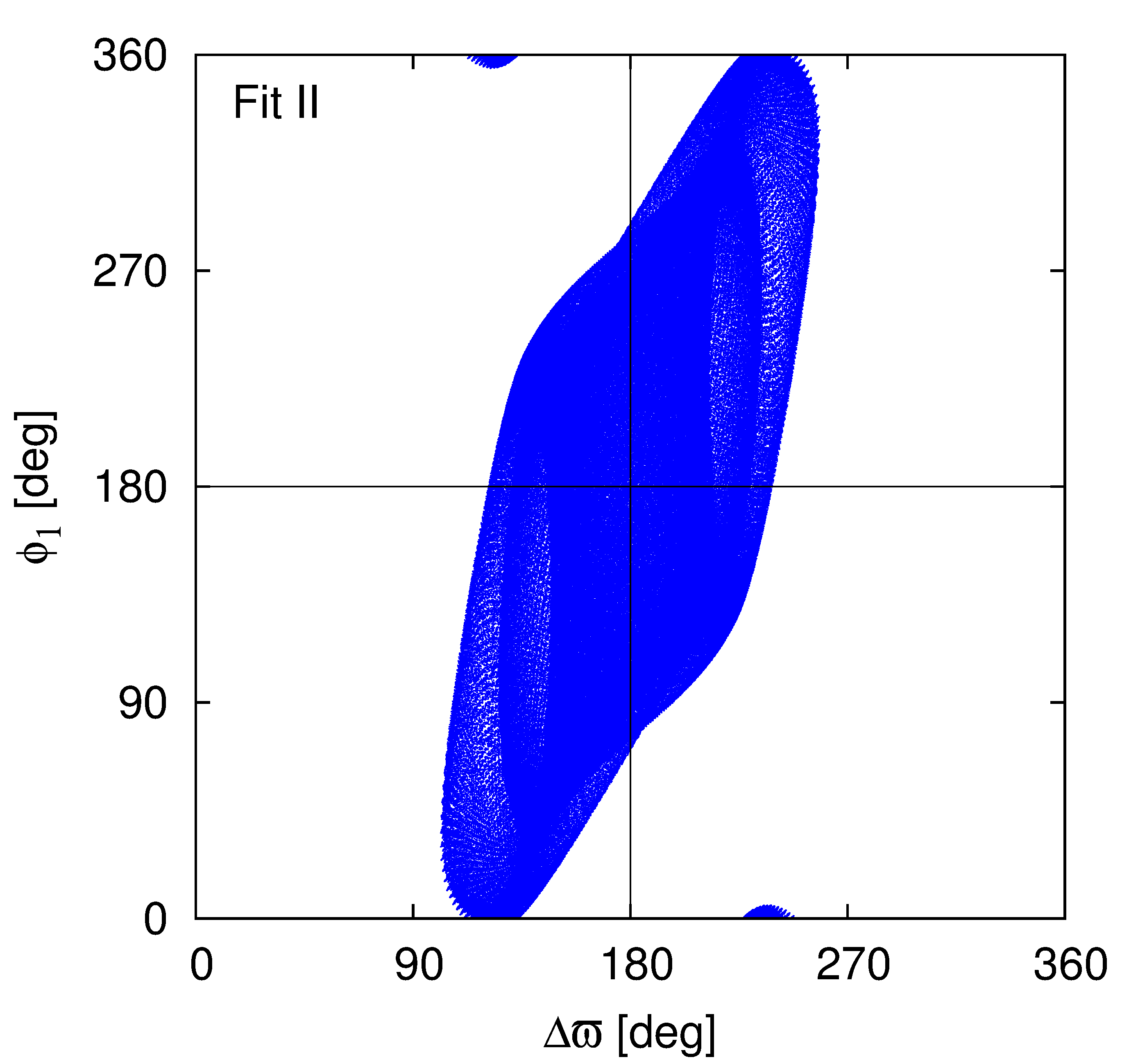
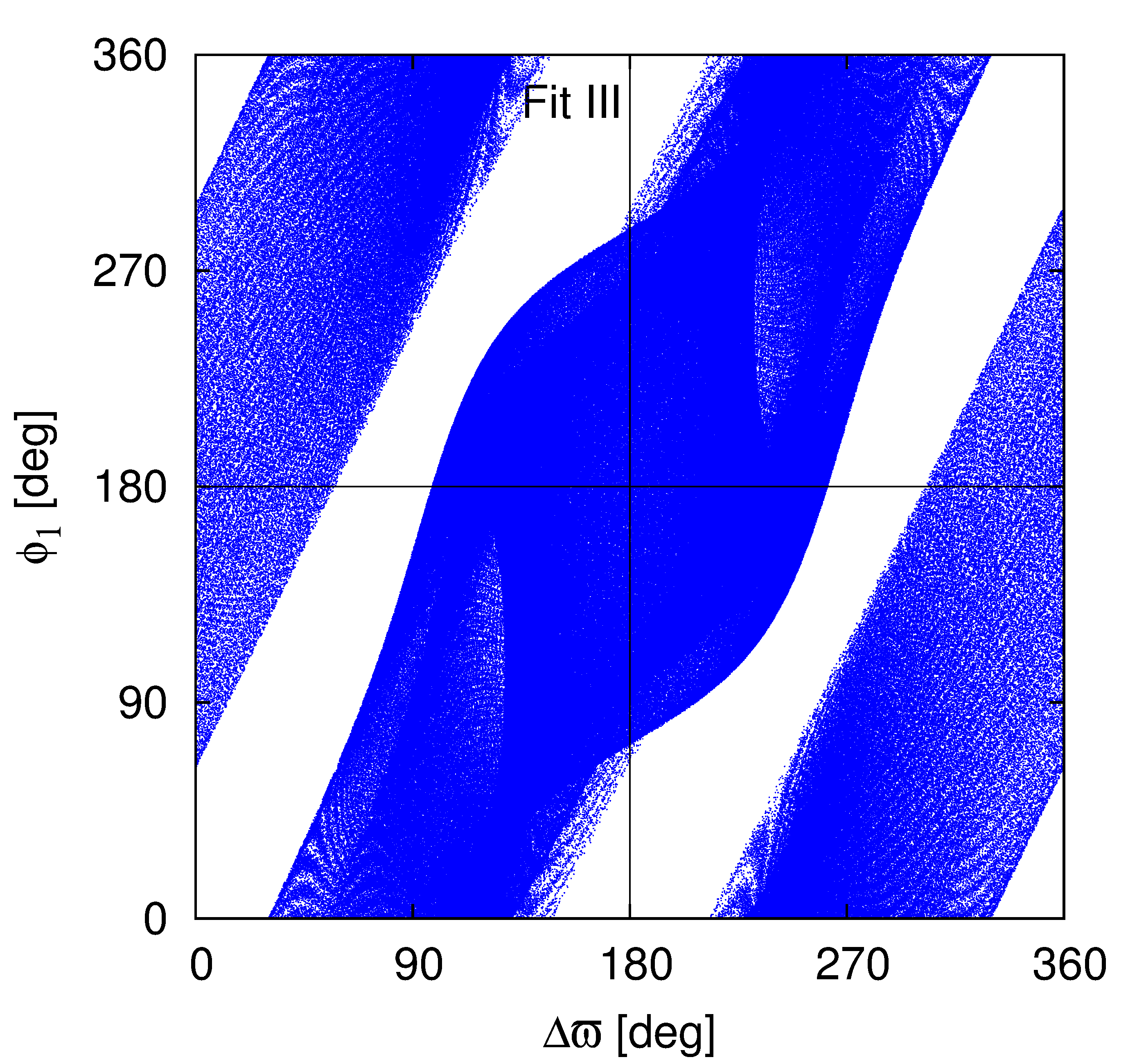
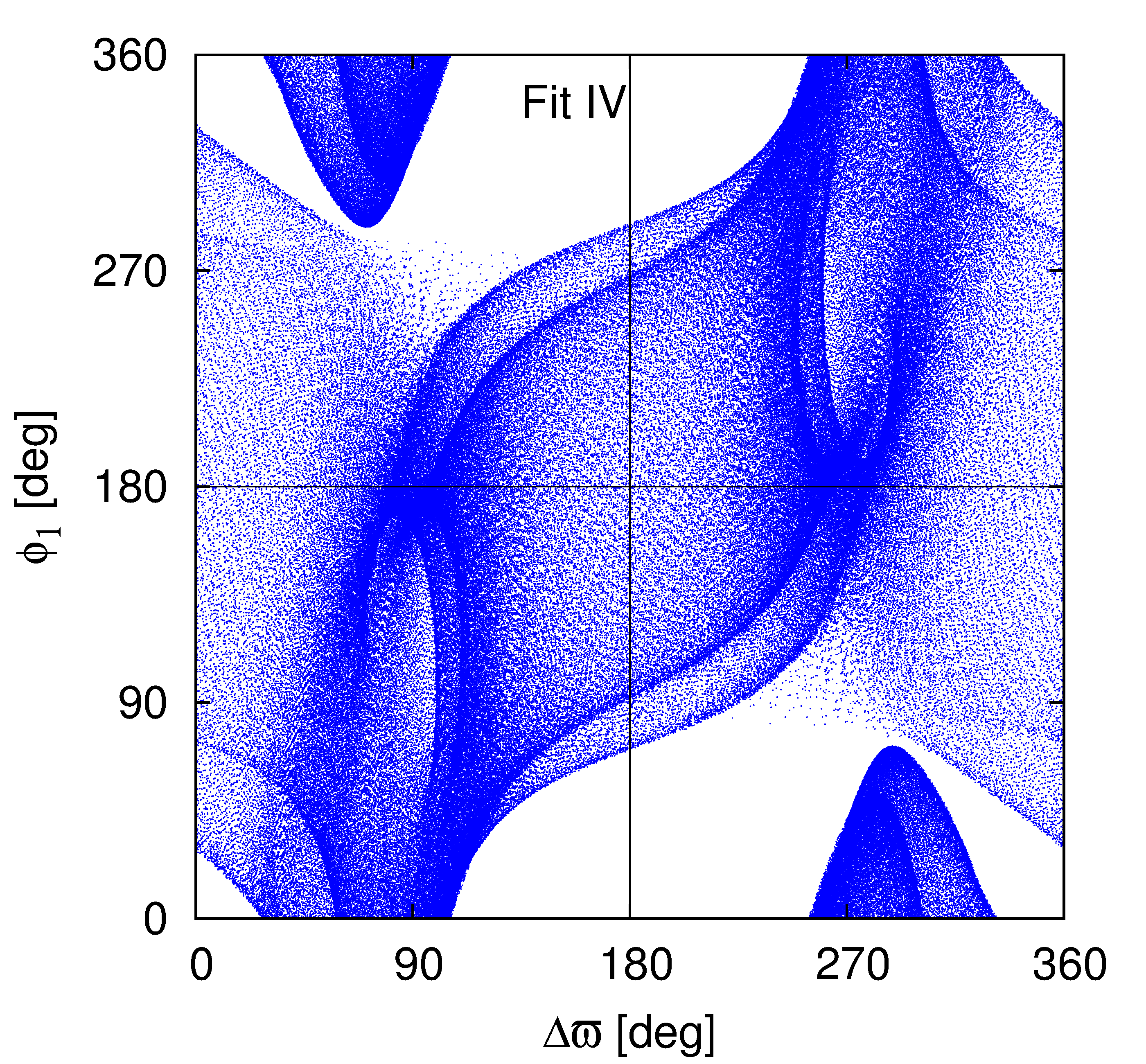
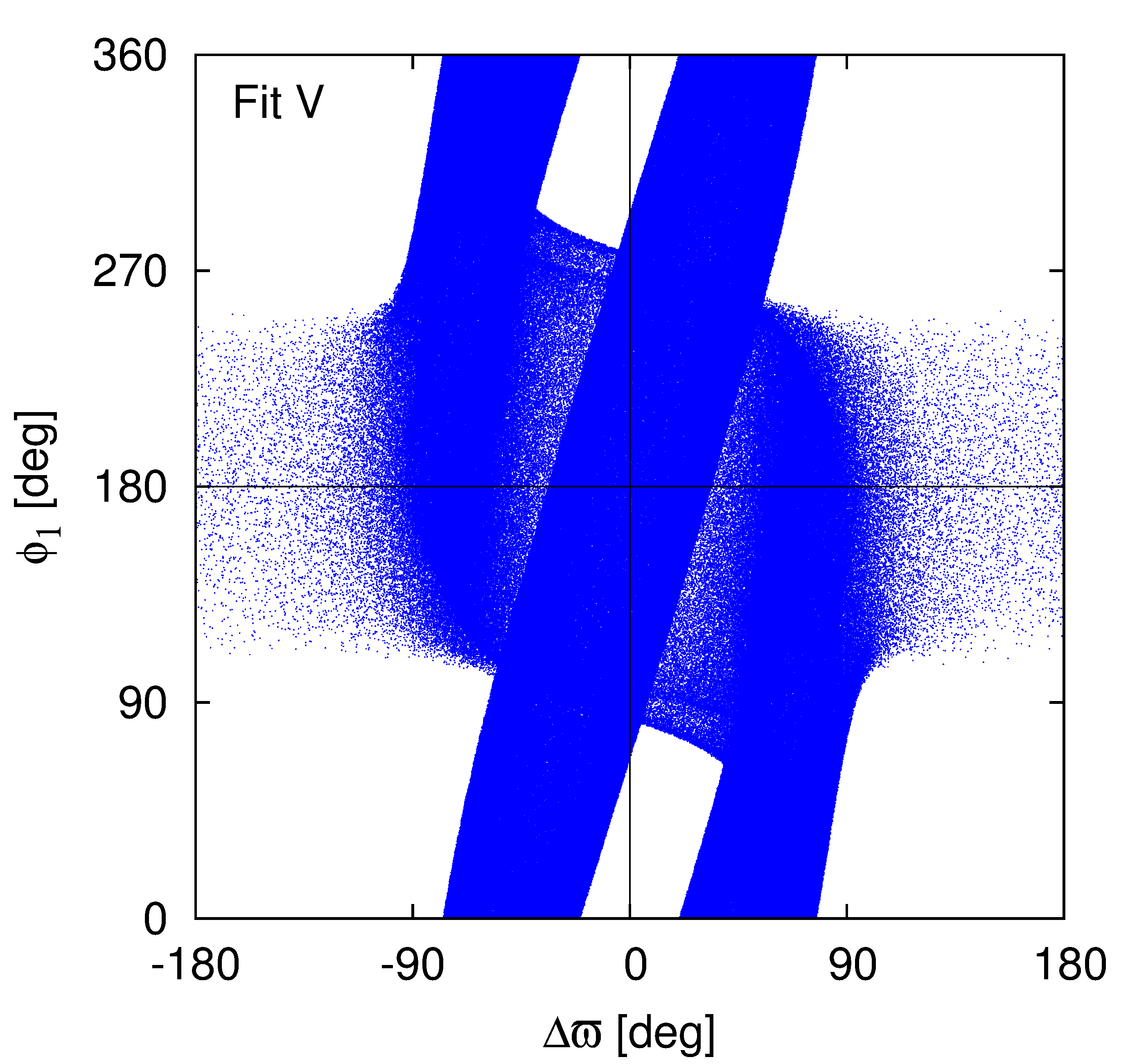
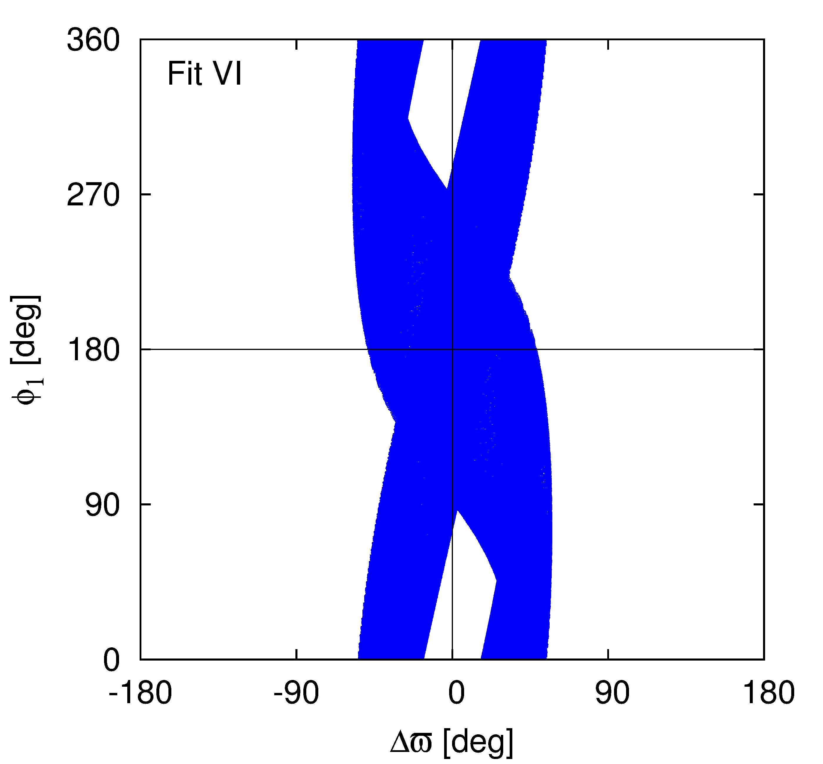
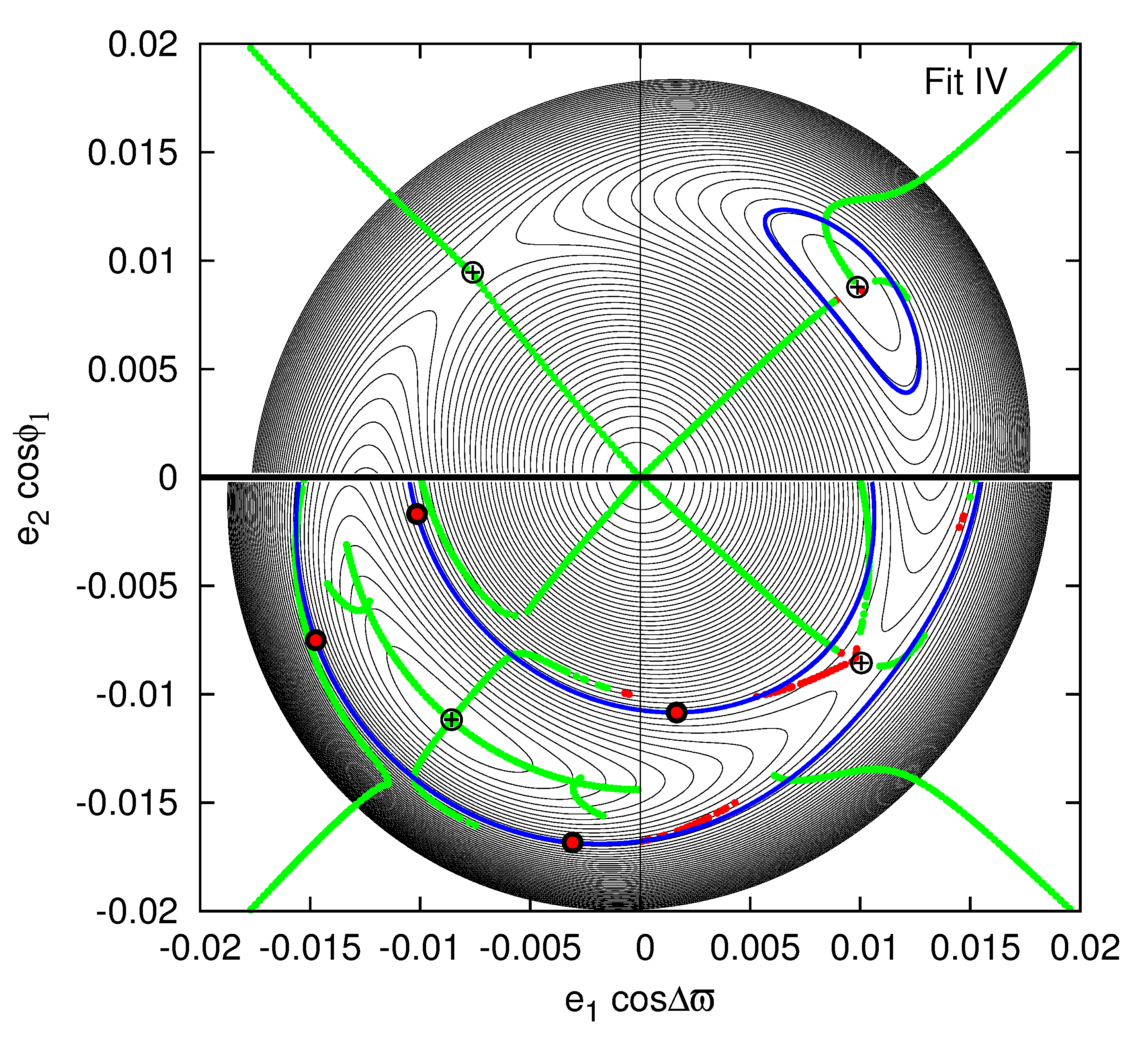
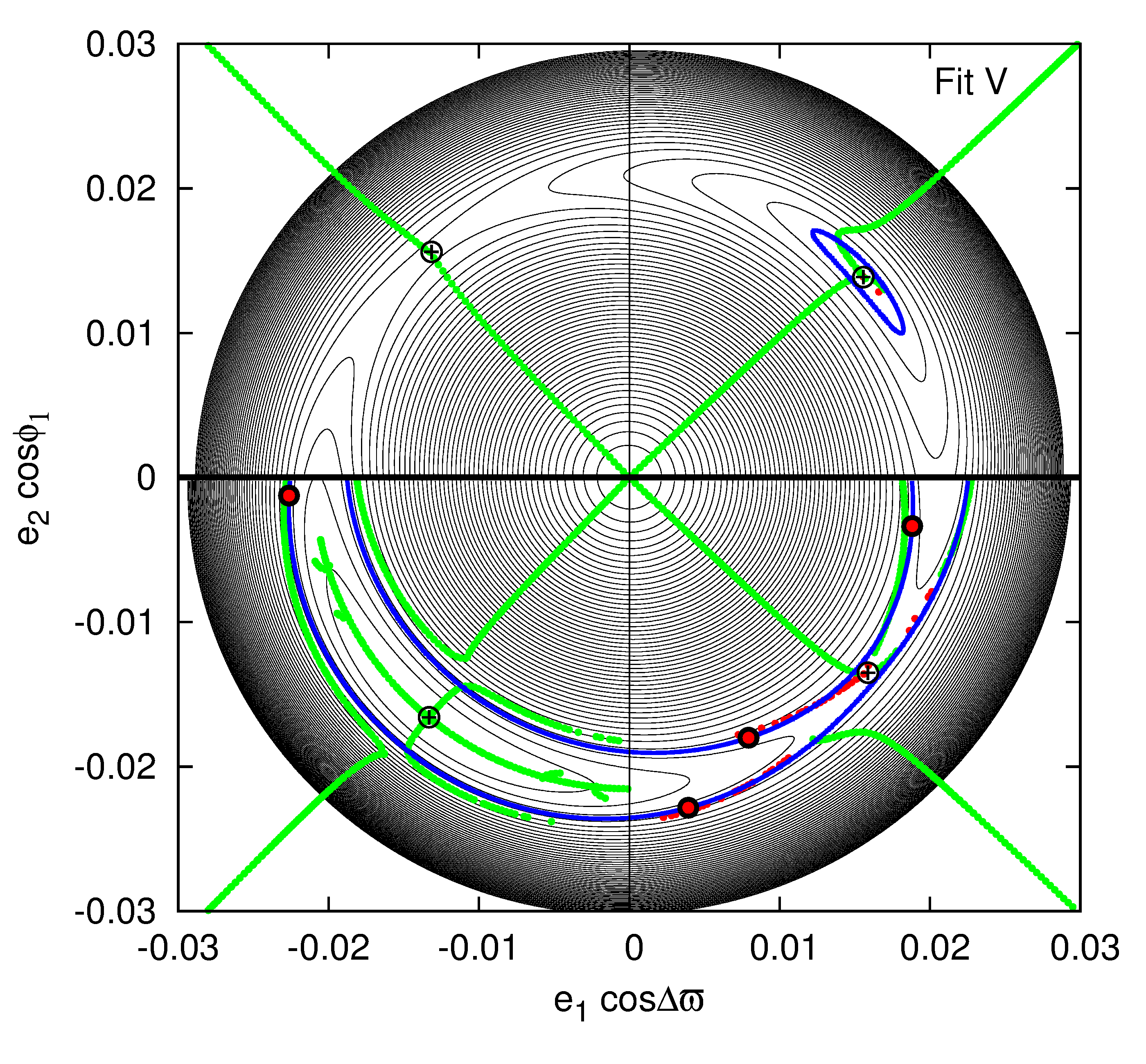
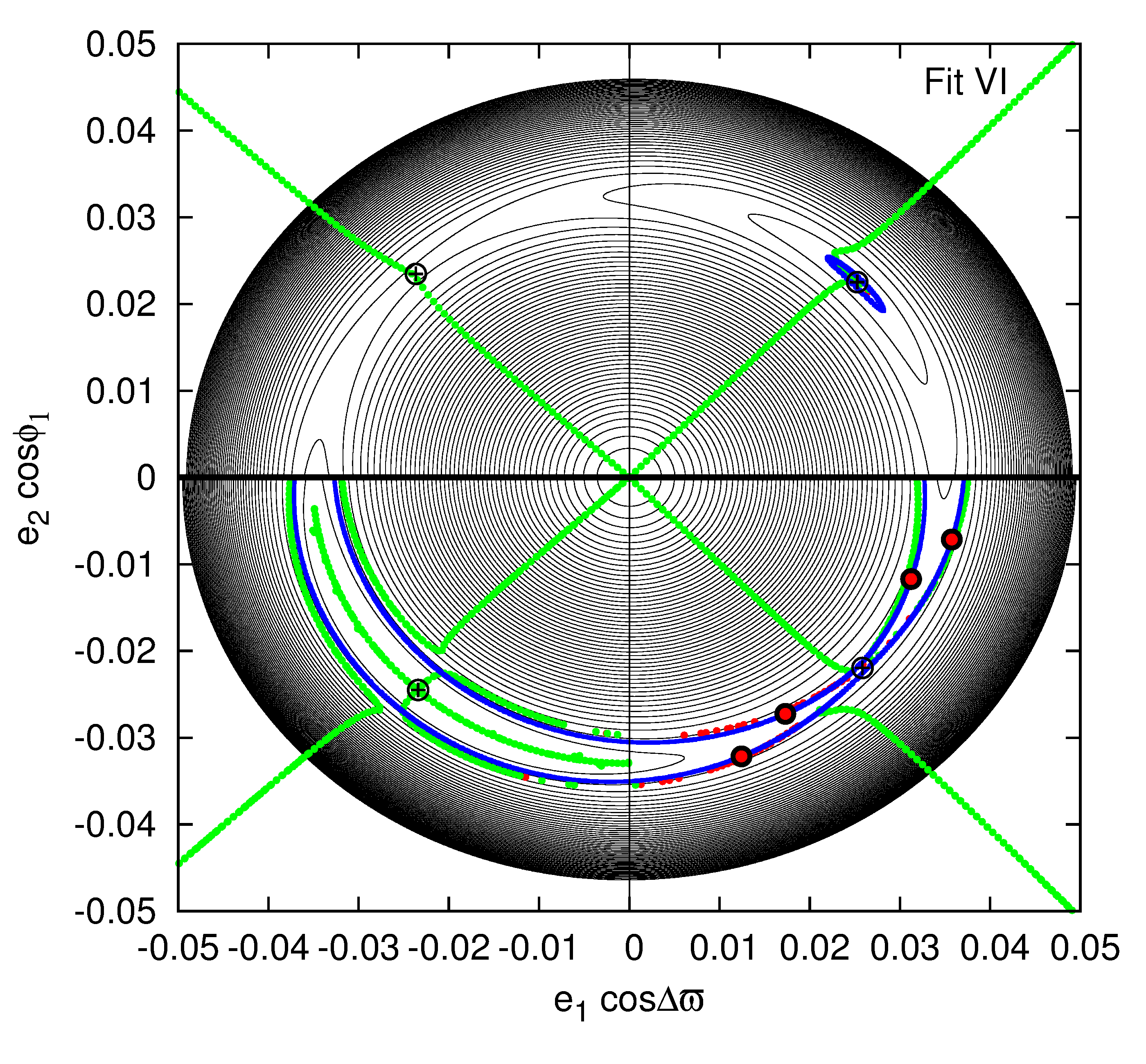
Figure 9 shows the orbital evolution of the selected models at the -plane. Both angles of Fit I librate around , although the amplitude of libration is large. For the second model in the test sample (Fit II), the libration amplitude reaches , while librates with a moderate amplitude. Since the amplitude of is actually greater than , we could classify the behaviour of this angle as circulation. Despite of the formal rotation of , the phase-space trajectory of Fit II intersects only one quarter of plane with . The next Fit III in the sample exhibits both critical angles rotating and two quarters of plane are intersected by the phase trajectory. Two other quarters are being avoided. Similarly, the phase trajectory of Fit IV intersects the same two quarters of plane. Yet the behaviour of the angles is different. For Fit IV, seems to librate but with an amplitude larger than . The next system, Fit V, shows both angles circulating, however in this case remains mainly around during the evolution, only occasionally reaching . The last model, Fit VI, has librating around and circulating.
Similarly to Fig. 8, Fig. 9 also reveals the transition between two different types of configurations (from Fit I to Fit VI). The sequence of the configurations can be also analysed in energy plots of the averaged system presented in Fig. 10. Mean orbital parameters of Fit I to Fit VI are displayed in Tab. 3.
| model/pl | [deg] | [deg] | |||
|---|---|---|---|---|---|
| I/b | |||||
| I/c | |||||
| II/b | |||||
| II/c | |||||
| III/b | |||||
| III/c | |||||
| IV/b | |||||
| IV/c | |||||
| V/b | |||||
| V/c | |||||
| VI/b | |||||
| VI/c |
A given energy plot is constructed for values of the two integrals and computed for each studied system. The energy of each system is determined by the averaged Hamiltonian (see Appendix A). Energy levels are plotted in the plane. The energy level for the nominal system is plotted with blue solid curve, while black solid curves are for other values of the energy, from the maximum of the energy that corresponds to the stable equilibrium (black cross-circle symbol in the -quarter of plane), down to smaller values. The energy levels are limited from the bottom by . The levels could be plotted also for smaller values, although these levels would become subsequently denser and they would be placed further from the centre of the plane. Other three cross-circle symbols in the remaining quarters represent positions of the unstable equilibria.
Let us recall that Fig. 8 shows positions of equilibria of the averaged system (periodic orbits of the full, non-average -body model of motion) computed not for one particular value of , like in Fig. 10, but for a series of values. This leads to whole branches/families of equilibria shown with green and red curves for stable and unstable equilibria, respectively. On contrary, green and red curves in Fig. 10 represents periodic orbits of the averaged system, green are for stable, while red – for unstable configurations. Big red/black symbols point where the nominal systems intersect the planes. The points of intersections can be compared with the ones in the right-hand panel of Fig. 8. Small differences are present between the results of the -body and the averaged model, which may be easily explained. The averaged model is of the first order w.r.t. the perturbation, which do not have to be necessarily small for such a compact two-planet system. Nevertheless, a sequence of models from Fit I (close to the stable equilibrium) to Fit VI (close to the unstable equilibrium) is apparent here as well.
A common feature of all the models is a close proximity of their nominal energy curves to the bifurcation of the branches of periodic orbits of the averaged system in the -quarter (see the arrows in the top left-hand panel of Fig. 10). Moreover, the energy values are just below the critical energy of the saddle point in the -quarter. Naturally, those two characteristics of the energy for the nominal systems, are not independent one from another, since the structure of periodic orbits is determined by positions of the equilibria. This feature may be a ”fingerprint” of the migration scenario, which we discuss in the next Section.
| solution/planet | [deg] | |||
|---|---|---|---|---|
| I/b | ||||
| I/c | ||||
| II/b | ||||
| II/c | ||||
| III/b | ||||
| III/c | ||||
| IV/b | ||||
| IV/c | ||||
| V/b | ||||
| V/c | ||||
| VI/b | ||||
| VI/c |
4 Planetary migration
To reproduce the observational Kepler-29 system, and its features discussed in Section 3, we conducted migration simulations within a simple parametric model of the force which mimics the planet-disc interactions (e.g., Beaugé et al., 2006; Moore et al., 2013)
| (4) |
where is the astrocentric velocity of planet (), is the velocity at circular orbit at a distance of planet . The time-scales of migration and circularisation of planet are denoted by and , respectively.
![[Uncaptioned image]](/html/1609.09135/assets/fig7.png)
We assumed that , where is constant and
| (5) |
where , and are constant. The free parameters of the model were being changed in wide ranges, i.e., , , , . Initial orbits were chosen such that the period ratio was between and , the eccentricities , and the angles were chosen to be . The choice of the initial period ratio smaller than stems from the fact that for initial , the system would very likely enter 4:3 MMR, taking the migration parameters from the ranges given above.
After a series of simulations we found the following properties of systems stemming from the migration. For small , moderate and high eccentricities () were possible to obtain, however librates around , which is opposite to the results of fitting the data. Additionally, such systems have always librating around . Both the angles librate around . For moderate , small eccentricities are obtained and spans the whole range, revealing both librations around or circulations, which agrees with the statistics of models that fit the data.
Next, we tried to find configurations resulting from the convergent migration, which could form the sequence of six models analysed in the previous Section. They should transform from one class of configurations (close to the stable equilibrium) to another class (close to the unstable equilibrium).
After a series of experiments, we found that three out of six models could be qualitatively reconstructed by a single migration simulation. The results of such a simulation are illustrated in Fig. 11. Its parameters as well as the initial orbital elements are given in the caption to this Figure. Subsequent panels, from the top to the bottom, correspond to the period ratio, eccentricities, and evolution in time. Shortly after the system reaches the 9:7 MMR, the eccentricities are excited, i.e., oscillates in a range of and . Both critical angles librate around , with very small amplitude , while with much larger amplitude of . Both the amplitudes increase in the first part of the simulation kyr. If the migration has stopped for some reason at this stage of the evolution, would librate with too small amplitude, when compared to the examples listed in Tab. 2 and also to the systems from the whole statistics of the TTV fits.
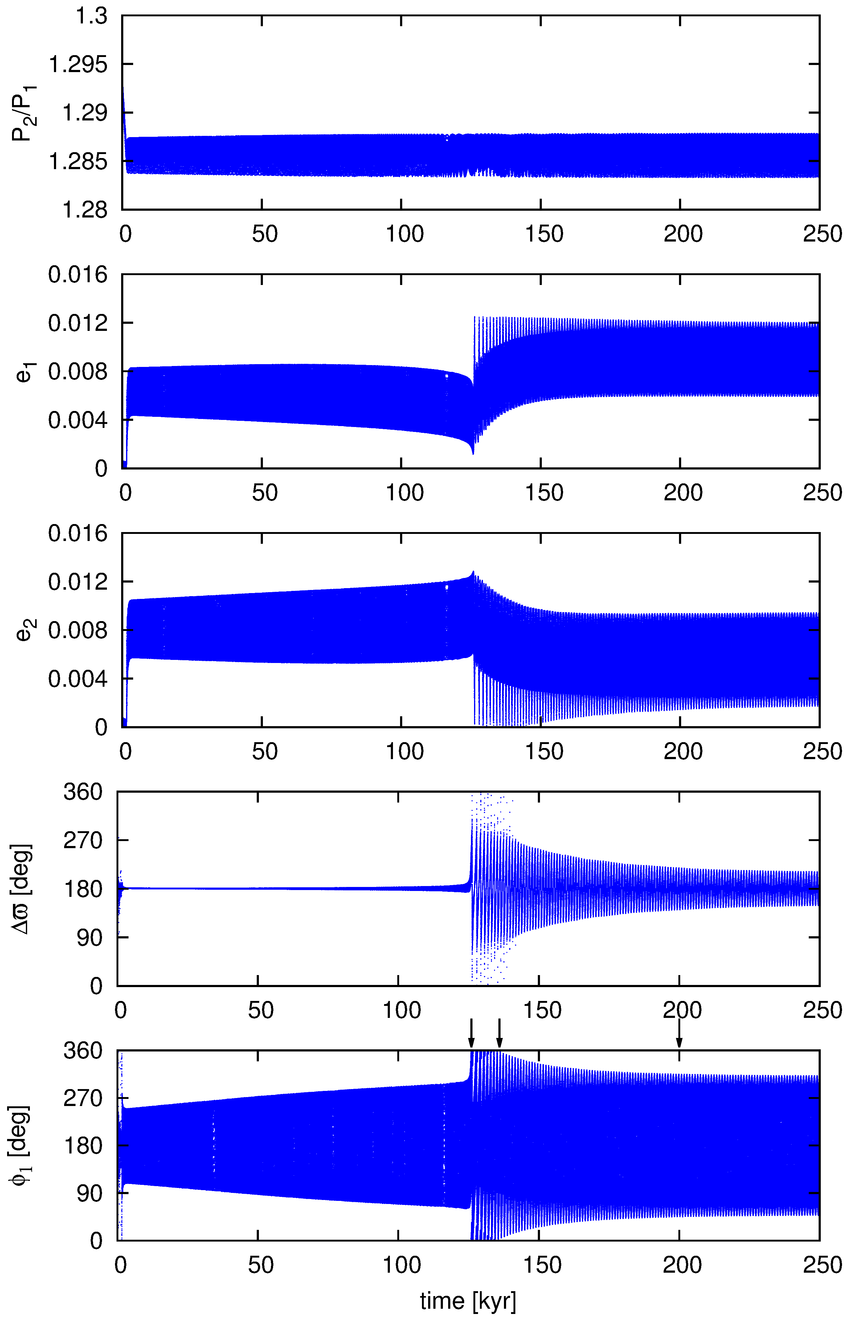
At kyr the system switches into a different regime of motion. Both and start to circulate, the ranges of the eccentricities oscillations also change. After kyr since the transition (at kyr) the angles start to librate again with decreasing amplitudes. One should keep in mind, though, that it is not a generic situation. If had a higher value (which would mimic slower disc dispersion), the system would leave the resonance eventually. If, on the other hand, was smaller, the migration could stop before the transition between the two discussed regimes of motion.
More details about the evolution of a system trapped in 9:7 MMR could be found in our upcoming paper. Here we only present an example showing that systems listed in Tab. 2 can be formed through the migration. A critical issue is the transition described above. It occurs if the energy of the migrating system reaches the bifurcation of the branches of periodic orbits (see the arrows in the top left-hand panel of Fig. 10).
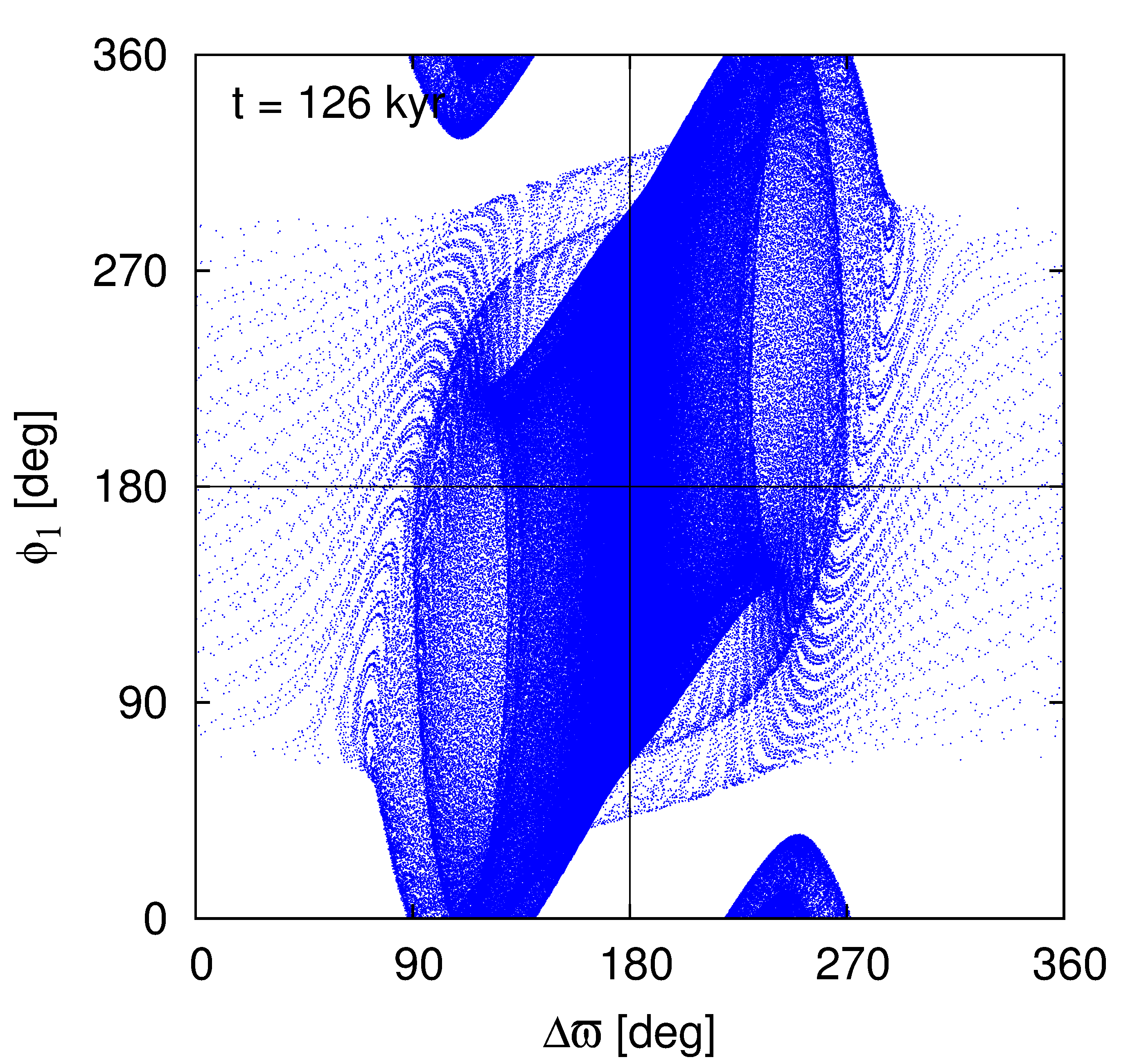
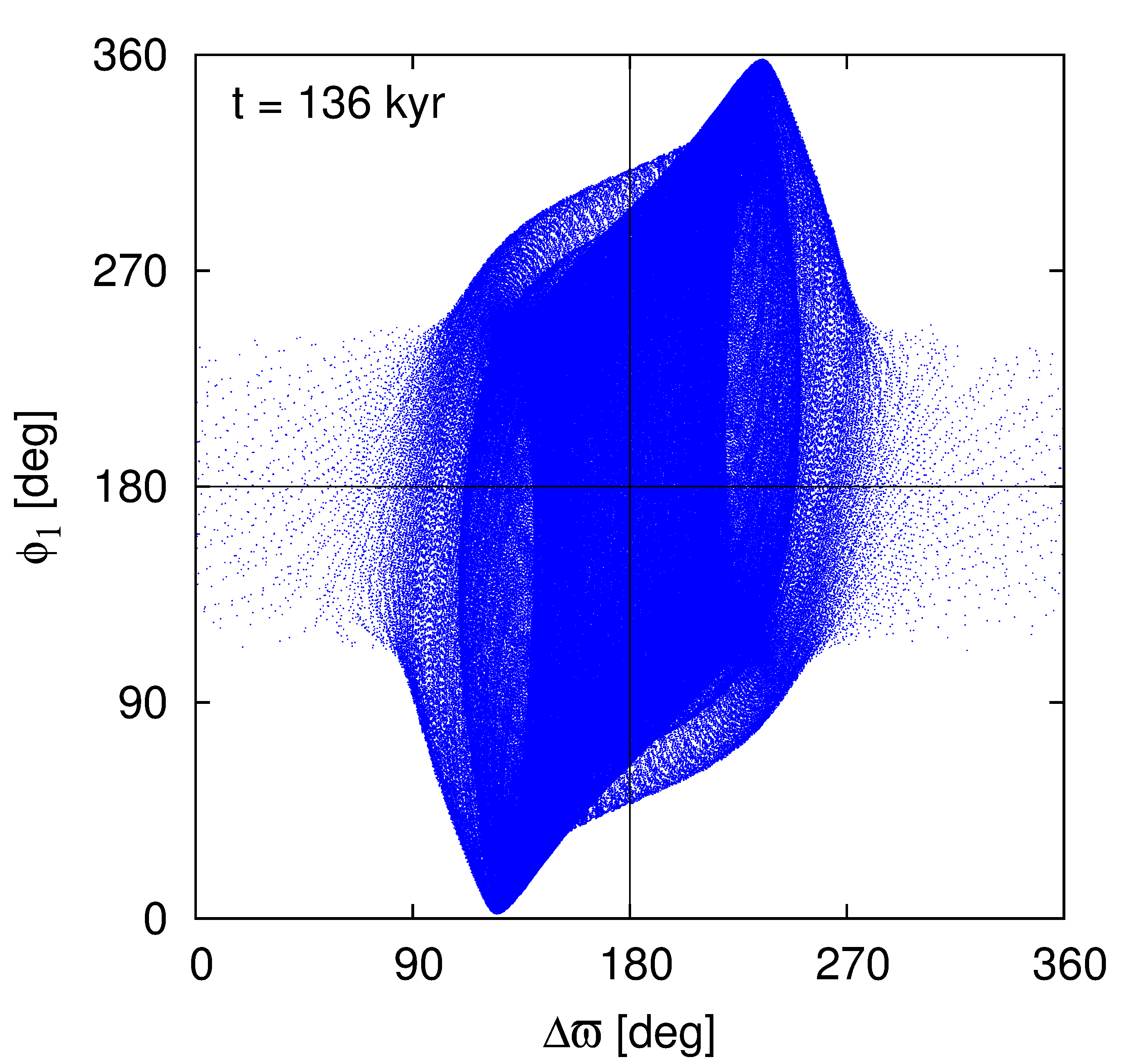
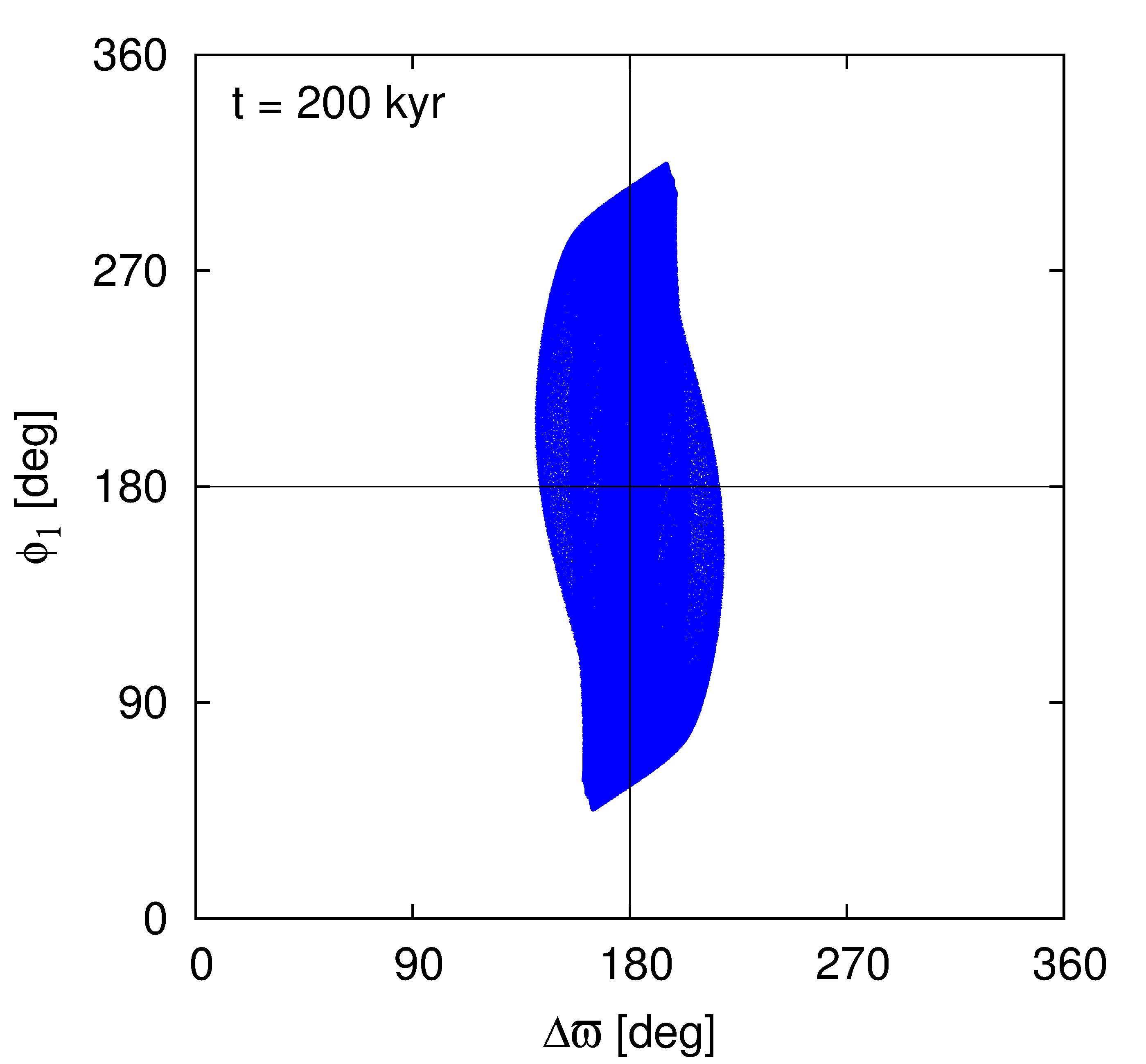
We chose three moments of the simulation, and kyr, respectively, and we integrated the -body equations of motion for the three sets of the osculating Keplerian elements at those epochs. Snapshots of their evolution are presented at the -diagrams in Fig. 12.
The left-hand panel reminds the bottom left-hand panel of Fig.9 (Fit IV) as well as the middle panel of Fig. 5 for the observational model close to the best-fitting solution in Tab. 1. Both the angles formally circulate, however, similarly to Fit IV, librates with the amplitude greater than . The evolution of the angles is not independent one from another, since the phase trajectory avoids certain areas of the -diagram. The right-hand panel of Fig. 12 reminds the top left-hand panel of Fig. 9 (Fit I). Both the angles librate and the amplitudes for the simulated system correspond well to the amplitudes for Fit I. The system in the middle panel can be interpreted as an intermediate state between the systems illustrated in the left and right panels of Fig. 12. The amplitude of libration reaches , which corresponds to the behaviour of Fit II (the top middle panel of Fig. 9). The only difference between the simulated system and Fit II is the behaviour of . Yet we also note that the evolution of critical angles for Fits V and VI is very similar to the observational models illustrated in the left and right panels of Fig. 6.
The examples stemming from the migration simulation ensure us that the Kepler-29 system could be formed by the planetary migration if its orbits are close to circular. On the other hand, the systems with higher eccentricities (and aligned orbits) which are also consistent with the TTV observations are less likely to be formed in this way. Nevertheless, the migration induced formation of the 9:7 MMR as well as other second- and higher-order resonances is a very complex mechanism. It needs to be studied in more details in order to bring a definitive solution.
5 Conclusions
We analysed the TTV data from (Rowe et al., 2015) of the Kepler-29 system with two low-mass planets of a period ratio very close to 9/7 (Jontof-Hutter et al., 2016). We confirmed that the masses of the planets are within a few Earth mass range, i.e., and for the inner and the outer planet, respectively. We demonstrated that, although the eccentricities as well as longitudes of pericenters are not well determined, the system is very likely in an exact 9:7 MMR. We found configurations with both aligned and anti-aligned apsides, that are long-term stable and fit the data equally well. The eccentricities may be as high as for models with aligned orbits, while for anti-aligned configurations only low eccentric orbits are allowed by the observational and stability constraints.
We demonstrated that the critical angles of the resonant configurations do not necessarily librate. That implies also that the secular angle may both rotate or librate, around or . The resonant nature of such systems can be verified at the frequency maps (right-hand column of Fig. 5) as well as at the -diagrams (Fig. 9). The fundamental frequencies related to the mean motions are very close to the nominal value of 9/7 for the systems whose resonant angles rotate. Moreover, the evolution of the angles and is correlated.
We showed that the best-fitting solutions with low eccentricities (both with aligned and anti-aligned apsides) are shifted with respect to the periodic orbits (equilibria of the averaged system) of 9:7 MMRs, and demonstrated that it is a natural outcome of the planetary migration. That holds even for configurations that lie close to the branch unstable periodic orbits for (Fit IV). On the other hand, we showed that configurations with and are unlikely to be formed on the way of migration. Systems with and can form this way, but configurations of this sort do not fit the TTV observations. Therefore, we conclude that if the Kepler-29 system was formed through the smooth migration, its orbits are low eccentric , but the behaviour of and the resonant angles can be hardly determined on basis of the available TTV data.
6 Acknowledgements
We would like to thank the anonymous referee for helpful suggestions that helped us to improve the paper. We thank Ewa Szuszkiewicz, John Papaloizou and Zija Cui for discussions stimulating our interest in the Kepler-29 dynamics. This work has been supported by Polish National Science Centre MAESTRO grant DEC-2012/06/A/ST9/00276. K.G. thanks the staff of the Poznań Supercomputer and Network Centre (PCSS, Poland) for a generous support and computing resources (grant No. 195).
Appendix A Analytic 9:7 MMR Hamiltonian
The secular and the resonant parts of the averaged Hamiltonian (Eq. 3) read as follows (Murray & Dermott, 1999).
The secular Hamiltonian is expressed through,
where are functions of the semi-major axes ratio through the Laplace coefficients and their derivatives. They read
where
| (7) |
Resonant terms that remain after averaging the expansion of the perturbing function,
where coefficients are specified as follows:
References
- Agol et al. (2005) Agol E., Steffen J., Sari R., Clarkson W., 2005, MNRAS, 359, 567
- Baluev (2009) Baluev R. V., 2009, MNRAS, 393, 969
- Beaugé et al. (2003) Beaugé C., Ferraz-Mello S., Michtchenko T. A., 2003, ApJ, 593, 1124
- Beaugé & Michtchenko (2003) Beaugé C., Michtchenko T. A., 2003, MNRAS, 341, 760
- Beaugé et al. (2006) Beaugé C., Michtchenko T. A., Ferraz-Mello S., 2006, MNRAS, 365, 1160
- Carter et al. (2011) Carter J. A., Fabrycky D. C., Ragozzine D., Holman M. J., Quinn S. N., et al. 2011, Science, 331, 562
- Charbonneau (1995) Charbonneau P., 1995, ApJS, 101, 309
- Cincotta et al. (2003) Cincotta P. M., Giordano C. M., Simó C., 2003, Physica D Nonlinear Phenomena, 182, 151
- Deck et al. (2014) Deck K. M., Agol E., Holman M. J., Nesvorný D., 2014, ApJ, 787, 132
- Fabrycky et al. (2012) Fabrycky D. C., Ford E. B., Steffen J. H., Rowe J. F., Carter J. A., Moorhead A. V., Batalha N. M., Borucki W. J., Bryson S., Buchhave L. A., et al. 2012, ApJ, 750, 114
- Ferraz-Mello et al. (2003) Ferraz-Mello S., Beaugé C., Michtchenko T. A., 2003, Celestial Mechanics and Dynamical Astronomy, 87, 99
- Foreman-Mackey et al. (2013) Foreman-Mackey D., Hogg D. W., Lang D., Goodman J., 2013, PASP, 125, 306
- Goodman & Weare (2010) Goodman J., Weare J., 2010, Comm. Apl. Math and Comp. Sci., 1, 65
- Goździewski & Migaszewski (2014) Goździewski K., Migaszewski C., 2014, MNRAS, 440, 3140
- Goździewski et al. (2016) Goździewski K., Migaszewski C., Panichi F., Szuszkiewicz E., 2016, MNRAS, 455, L104
- Hadden & Lithwick (2014) Hadden S., Lithwick Y., 2014, ApJ, 787, 80
- Hadjidemetriou (2006) Hadjidemetriou J. D., 2006, Celestial Mechanics and Dynamical Astronomy, 95, 225
- Holczer et al. (2016) Holczer T., Mazeh T., Nachmani G., Jontof-Hutter D., Ford E. B., Fabrycky D., Ragozzine D., Kane M., Steffen J. H., 2016, ApJS, 225, 9
- Jontof-Hutter et al. (2016) Jontof-Hutter D., Ford E. B., Rowe J. F., Lissauer J. J., Fabrycky D. C., Van Laerhoven C., Agol E., Deck K. M., Holczer T., Mazeh T., 2016, ApJ, 820, 39
- Kane et al. (2012) Kane S. R., Ciardi D. R., Gelino D. M., von Braun K., 2012, MNRAS, 425, 757
- Laskar (1993) Laskar J., 1993, Celestial Mechanics and Dynamical Astronomy, 56, 191
- Lee et al. (2013) Lee M. H., Fabrycky D., Lin D. N. C., 2013, ApJ, 774, 52
- Michtchenko et al. (2006) Michtchenko T. A., Beaugé C., Ferraz-Mello S., 2006, Celestial Mechanics and Dynamical Astronomy, 94, 411
- Michtchenko & Ferraz-Mello (2001) Michtchenko T. A., Ferraz-Mello S., 2001, Icarus, 149, 357
- Migaszewski (2015) Migaszewski C., 2015, MNRAS, 453, 1632
- Moore et al. (2013) Moore A., Hasan I., Quillen A. C., 2013, MNRAS, 432, 1196
- Moorhead et al. (2011) Moorhead A. V., Ford E. B., Morehead R. C., et al. 2011, ApJS, 197, 1
- Morbidelli (2002) Morbidelli A., 2002, Modern celestial mechanics : aspects of solar system dynamics. Taylor & Francis, London and New York
- Morbidelli & Moons (1993) Morbidelli A., Moons M., 1993, Icarus, 102, 316
- Mullally et al. (2015) Mullally et al. 2015, ApJS, 217, 31
- Murray & Dermott (1999) Murray C. D., Dermott S. F., 1999, Solar system dynamics. Cambridge Univ. Press, Cambridge
- Plavchan et al. (2014) Plavchan P., Bilinski C., Currie T., 2014, PASP, 126, 34
- Rowe et al. (2015) Rowe J. F., Coughlin J. L., Antoci V., Barclay T., Batalha N. M., Borucki W. J., Burke C. J., et al. 2015, ApJS, 217, 16
- Ruciński et al. (2010) Ruciński M., Izzo D., Biscani F., 2010, ArXiv e-prints: 1004.4541
- Šidlichovský & Nesvorný (1996) Šidlichovský M., Nesvorný D., 1996, Celestial Mechanics and Dynamical Astronomy, 65, 137
- Van Eylen & Albrecht (2015) Van Eylen V., Albrecht S., 2015, ApJ, 808, 126
- Xiang-Gruess & Papaloizou (2015) Xiang-Gruess M., Papaloizou J. C. B., 2015, MNRAS, 449, 3043