Effect of long-range interactions on the phase transition of Axelrod’s model
Abstract
Axelrod’s model with cultural features, where each feature can assume states drawn from a Poisson distribution of parameter , exhibits a continuous nonequilibrium phase transition in the square lattice. Here we use extensive Monte Carlo simulations and finite size scaling to study the critical behavior of the order parameter , which is the fraction of sites that belong to the largest domain of an absorbing configuration averaged over many runs. We find that it vanishes as with at the critical point and that the exponent that measures the width of the critical region is . In addition, we find that introduction of long-range links by rewiring the nearest-neighbors links of the square lattice with probability turns the transition discontinuous, with the critical point increasing from to , approximately, as increases from to . The sharpness of the threshold, as measured by the exponent for , increases with the square root of the number of nodes of the resulting small-world network.
pacs:
87.23.Ge, 89.75.Fb, 05.50.+qI Introduction
Axelrod’s model for the dissemination of culture takes into account two key ingredients of social dynamics Lazarsfeld_48 ; Castellano_09 ; Galam_12 , namely, social influence through which people become more similar when they interact and homophily, which is the tendency of individuals to interact preferentially with similar others Axelrod_97 . Explicitly, in Axelrod’s model the individuals are modeled by agents which are strings of cultural features of length , where each feature can adopt a certain number of distinct states. The cultural features of an agent determine its culture. The agents are fixed at the nodes of a network (regular lattice or complex network) and the interaction between two connected agents takes place with probability proportional to the number of states they have in common and always results in an increase of the similarity between them.
Whereas social influence is a main feature of the standard two-opinion voter model Ligget_85 and homophily has been allowed for in the three-opinion constrained voter model Vazquez_03 ; Vazquez_04 , the number of states – two and three, respectively – is not a free parameter in those models. As a result, the two-opinion voter model exhibits only consensus absorbing configurations in regular lattices of arbitrary dimension Ligget_85 (see, however, Castellano_03 for a report of incomplete ordering on small-world networks). The same conclusion holds for the constrained voter model in an infinite one-dimensional lattice (see, e.g., Lanchier_12a ; Lanchier_12b ; Vilone_02 ; Biral_15 ) and since increasing the range of the agents’ interactions favors the consensus regime Greig_02 ; Klemm_03a , we expect this conclusion to hold for regular lattices of higher dimension as well. In Axelrod’s model, however, increase of the number of states for a fixed string length leads the social dynamics to freeze in multicultural absorbing configurations even in a one-dimensional lattice Lanchier_12b ; Vilone_02 .
In fact, Axelrod’s model exhibits two types of absorbing configurations in the thermodynamic limit : ordered configurations, which are characterized by a few cultural domains of macroscopic size , and disordered configurations, where all domains are microscopic Castellano_00 ; Klemm_03 ; JEDC_05 ; Vazquez_07 ; Peres_15 . By cultural domain we mean a bounded region of uniform culture. The competition between the disorder of the initial configuration that favors cultural fragmentation and the ordering bias of social influence that favors homogenization results in the nonequilibrium phase transition between those two classes of absorbing states Castellano_00 . We note that, similarly to the standard percolation Stauffer_92 , the phase transition occurs in the properties of the absorbing states and so it is static in nature Vilone_02 .
In this paper we reexamine the nonequilibrium phase transition of a variant of Axelrod’s model in which the initial states of the cultural features of the agents are drawn randomly from a Poisson distribution of parameter ,
| (1) |
with . In the original model, these states are chosen randomly from a uniform distribution on the integers Axelrod_97 . In the square lattice, the Poisson variant exhibits a continuous phase transition for and a discontinuous one for Castellano_00 . In the one-dimensional lattice, only the disordered regime exists for and a discontinuous transition between the disordered and the ordered regimes is observed for Vilone_02 . Here we focus on the case only and study the effect of long range interactions on the standard order parameter of Axelrod’s model that measures the fraction of agents that belong to the largest cultural domain, whose size is denoted by , averaged over many independent runs (see, e.g, Castellano_00 ; Vilone_02 ; Klemm_03a ).
A previous study of the continuous phase transition for in the square lattice considered as order parameter the mean density of domains , where denotes the number of domains of an absorbing configuration, and showed that it vanishes as with at the critical point Peres_15 . We note that is not an order parameter for the standard percolation since it is continuous and non-zero at the threshold Stauffer_92 . The advantage of considering is that it is nonzero in the disordered regime where the convergence of the dynamics to the absorbing configurations is very fast as compared to the convergence to the quasi-consensus configurations of the ordered regime (see, e.g., Biral_15 ). The present study complements that analysis by showing that the more usual order parameter vanishes at the critical point as with .
In addition, here we study the effect of long range interactions by considering small-world networks in which each link of the square lattice with periodic boundary conditions is rewired with probability . Rewiring of a link is done by replacing the original neighbor of a given site by a random site chosen uniformly among all possible sites that avoid self-loops and link duplication Watts_98 . The average degree of the resulting network is 4 regardless of the value of . The extremes and correspond to the regular square lattice and to a random network, respectively. Since the underlying regular lattice used to generate the small-world networks is the square lattice we can introduce the length , although it has no geometrical meaning for . We find that the transition is discontinuous for and that the critical exponent that determines the width of the critical region for finite is . However, in the case where the transition is continuous we find .
The remainder of the paper is organized as follows. For the sake of completeness, in Section II we present a brief account of Axelrod’s model Axelrod_97 and of the Watts and Strogatz algorithm for constructing small-world networks Watts_98 . In Section III we study the behavior of the order parameter near the critical region for three network topologies: the square lattice (), random networks () and small-world networks with rewiring probability . Finally, Section IV offers our concluding remarks.
II The Model
The Poisson variant of Axelrod’s model differs from the original model only by the procedure that generates the cultural states of the agents at the beginning of the simulation: for each feature of each agent a state is drawn independently using the distribution (1). Once the initial configuration is set, the dynamics proceeds as in the original model Axelrod_97 . In particular, at each time we pick an agent at random – the target agent – as well as one of its neighbors. These two agents interact with probability equal to their cultural similarity, defined as the fraction of common cultural features they have. An interaction consists of selecting at random one of the distinct features, and making the selected feature of the target agent equal to the corresponding feature of its neighbor. This procedure is repeated until the system is frozen into an absorbing configuration. According to these rules, at an absorbing configuration any pair of neighbors are either identical or completely different regarding their cultural states.
A feature that sets Axelrod’s model apart from most lattice models that exhibit nonequilibrium phase transitions Marro_99 is that all stationary states of the dynamics are absorbing states, i.e., the dynamics always freezes in one of these states. This contrasts with lattice models that exhibit an active state in addition to infinitely many absorbing states Jensen_93 and the phase transition occurs between the active state and the usually equivalent absorbing states (see Pace_14 for a simple change in the update rule of Axelrod’s model that results in dynamically active metastable states).
The implementation of the Watts and Strogatz algorithm Watts_98 for constructing the small-world networks used in our study begins with a square lattice of linear size with nearest neighbors interactions and periodic boundary conditions (i.e., a torus). Then for every site we rewire the link between and, say, its left neighbor, with probability . As mentioned before, rewiring of a link is done by replacing the original neighbor of site (in this case, the left neighbor) by a random site chosen uniformly among all possible sites that avoid self-loops and link duplication. The procedure is then repeated for, say, the top neighbor of every site of the lattice. Note that for the resulting network is not a classic random network Gilbert_59 , since the rewiring scheme guarantees that any site will be connected to at least other sites, whereas for classical random graphs any site has probability of being isolated from the other sites. Otherwise, the resulting networks are very similar to classical random graphs.
III Analysis of the order parameter
For a randomly generated initial configuration of the agents’ cultures, we follow the dynamics of Axelrod’s model until it reaches an absorbing state – this comprises a single run – and then we calculate the size of the largest cultural domain . Average of this quantity over a large number of independent runs (typically ), which differ by the choice of the initial cultural states of the agents as well as by their update sequence, yields the order parameter we use to characterize the nature of the absorbing configurations. In the case of random () and small world () networks we generate a different network for each run.
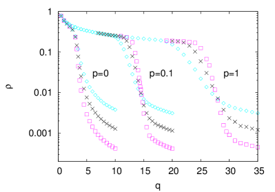
Figure 1 offers a bird’s eye view of the dependence of the order parameter on the parameter of the Poisson distribution, which determines the number of different cultural states in the initial population, for the three network topologies we will consider here, viz. the square lattice (), small-world networks with and random networks (). This figure reveals a few interesting features of Axelrod’s model. First, the presence of long range links favors the ordered regime as indicated by the shift of the threshold region to high values of , i.e., as the fraction of long-range links increases, the disorder in the initial configuration must also increase in order the dynamics reaches a disordered absorbing configuration Klemm_03a . Second, deep into the ordered phase, say for , the order parameter is completely insensitive to increasing the fraction of long-range links beyond a certain value, say . Third, the crossing of the data for different for signals the presence of a discontinuous transition in the limit , whereas for the condition for is satisfied for all values of .
Next we study in detail the behavior of the order parameter in the critical region for the three network topologies exhibited in Fig. 1.
III.1 Square lattice
The square lattice considered here exhibits only short range interactions and so it offers a baseline for assessing the effects of long-range links on the phase transition of Axelrod’s model. In addition, as pointed out before, this study complements previous analyses of the Poisson variant of Axelrod’s model in the square lattice Castellano_00 ; Peres_15 . In fact, whereas Ref. Castellano_00 considered the qualitative aspects of the continuous nonequilibrium transition (in the sense that there were no attempt to estimate the critical point and the critical exponents), Ref. Peres_15 focused on an alternative order parameter. Since we expect that the location of the critical point is not affected by the choice of the order parameter (in cases there is such choice), here we borrow from Peres_15 the estimate . The discernment of this resolution will be evaluated by the goodness and consistency of our results.
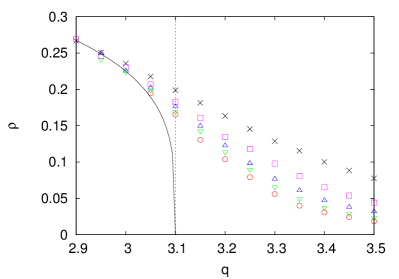
Figure 2 offers a more detailed view of the order parameter near the critical point . Rather remarkably, the finite size scaling theory asserts that for large the data shown in this figure can be described by the scaling relation Privman_90
| (2) |
where the scaling function is for and is a critical exponent that determines the width of the critical region for finite . Hence in the limit one has near the critical point, where is a critical exponent.
Figure 3 summarizes the results of the fitting of the data for with the function , where and are the two adjustable parameters of the fitting. The choice of the fitting region is determined by requiring that the fit curve goes through the data for as well. This procedure yields for the critical exponent that governs the vanishing of the order parameter at the critical point. The resulting fit curve is also shown in Fig. 2 using a linear scale.
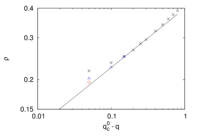
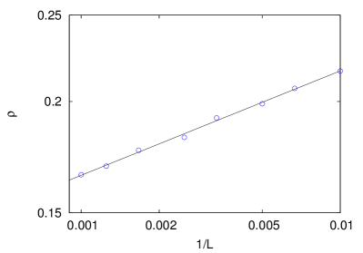
According to the scaling relation (2), must decrease to zero as the power law at and we explore this fact in Fig. 4, where is plotted against in a log-log scale, to determine the ratio . Finally we are now in position to estimate the exponent . The goodness of our estimates of the critical exponents as well as the judiciousness of borrowing the location of the critical point from Peres_15 can be assessed by checking whether the scaled quantity is independent of the lattice size when plotted against the scaled distance to the critical point as predicted by eq. (2). This is shown in Fig. 5. The quality of the collapse of the data for distinct lattice sizes supports heartily our estimates of the critical exponents.
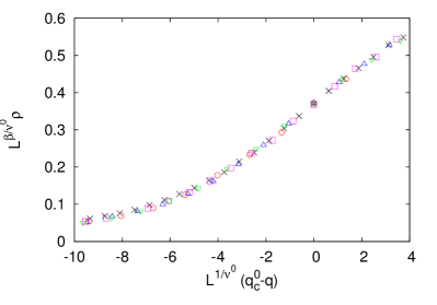
The two critical exponents and that determine the behavior of the order parameter in the critical region of Axelrod’s model set its continuous nonequilibrium phase transition apart from the known universality classes of nonequilibrium lattice models Marro_99 . This is probably due to the static nature of the transition and to the existence of infinitely many absorbing configurations in both – ordered and disordered – phases.
III.2 Random networks
To study the phase transition for random networks generated by the limit of sure rewiring (i.e., ) of the Watts and Strogatz algorithm Watts_98 we need first to obtain a good estimate of the location of the critical point . According to Fig. 1, in the limit one expects that for and for , so that the order parameter jumps from to at . Hence in order to determine , in Fig. 6 we plot against for several values of in the critical region. A rough estimate of this region is provided by Fig. 1, which also offers a good estimate for the jump at the critical point, . At the order parameter is independent of (hence the intersection of the data for different at the critical point), i.e., exhibits a plateau as . Although such plateaus exist for all since for large , there is no risk of confusing the two types of plateaus because the range of shown in Fig. 6 is about one order of magnitude smaller than . Visual inspection of Fig. 6 indicates that so we estimate .
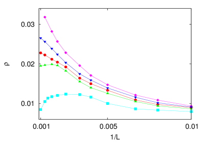
Figure 6 also illustrates the strong finite size effects that hinder the analysis of the order parameter in the critical region. Consider, for instance, the data for . If our analysis were restricted to that value of would be a good candidate for the critical point, because of the plateau observed in the range . In fact, the data for shown in Fig. 1 cross at about . Hence to probe the correct critical behavior of we must consider random networks with . This contrasts to our findings for the square lattice, for which the analysis of rather small networks (e.g., ) yields useful information about the critical behavior (see Figs. 3 and 5).
We focus now on the characterization of the sharpness of the threshold, i.e., the range of about where the threshold features persist. To achieve that we will assume that the critical region shrinks to zero like as , i.e., we will assume that the order parameter is described by the expression in the critical region. Here is a continuous function such that for and for . Our approach is in the same spirit of the finite-size scaling of combinatorial problems Kirkpatrick_94 ; Monasson_99 (see Campos_98 for a similar study in the context of the quasispecies model), for which there is no geometric criterion for defining a quantity analogous to a correlation length, and so the success of the method in accounting for the size dependence of the order parameter cannot be attributed to the divergence of a correlation length and the consequent onset of a second order phase transition. In addition, we recall that even the parameter has no geometric interpretation for random networks.
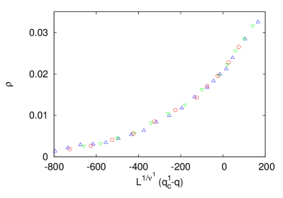
Figure 7 confirms that, in the critical region, the order parameter is a smooth function of the properly rescaled distance to the critical point. The estimate for the critical exponent was obtained by requiring that the data for distinct collapse into a single curve, the function . In particular, we find , as expected (see Fig. 6). The uncertainty of the estimate of can be evaluated using the same procedure, i.e., by gauging the quality of the data collapse as the exponent departs from . We find very poor data collapses for exponents outside the range (data not shown). This figure reveals also our difficulty to obtain reliable results in the ordered phase due to the very long convergence times Biral_15 . We conclude then that the sharpness of the transition increases with the square root of the number of agents, .
III.3 Small-world networks
We turn now to the analysis of the discontinuous transition for small-world networks with rewiring probability . Our aim is to verify whether the exponent , and hence the sharpness of the threshold, is influenced by the value of . Figure 1 indicates that in the limit the order parameter jumps from to at the threshold. The procedure used to determine the critical point is the same as that illustrated in Fig. 6 for random networks and yields . The finite size effects are also very strong in this case and so it is also necessary to resort to large networks, say , to assess the critical region.
In Fig. 8 we examine the assumption that the order parameter satisfies in the critical region. As before, is such that for and for . The best collapse of the data for distinct is obtained with and it is shown in the figure. The uncertainty of the exponent is estimated as before, i.e., by varying around and gauging the quality of the resulting data collapse. In addition, Fig. 8 shows that , implying that the data for different intersect at in the plane .
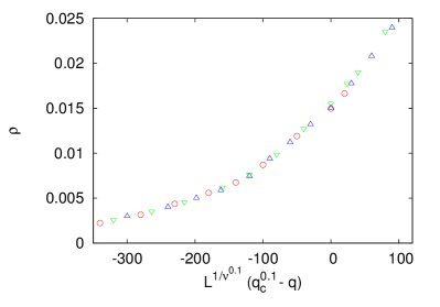
We have also considered values of rewiring probability down to and verified that the order parameter when plotted against for different values of (see Fig. 1) always cross at some value , thus signalling the existence of a discontinuous transition between the ordered () and the disordered () phases. Although we have estimated the sharpness of the threshold for and only, the observed irresponsiveness of the exponent to this tenfold decrease of prompt us to conjecture that this exponent is a universal feature of the discontinuous transitions of Axelrod’s model with two cultural features () in small-world networks.
IV Conclusion
Axelrod’s model exhibits a good balance between simplicity and realism, being considered a choice model to study collective social phenomena from a quantitative perspective Goldstone_05 . For instance, Axelrod’s model has proven useful to study the effects of global media on the polarization of public opinion Shibanai _01 ; Avella_10 ; Peres_11 ; Reia_16 as well as to understand the emergence of a collective intelligence from the local interactions between dumb agents Kennedy_98 ; Fontanari_14 . However, rather than explore the riveting applications of Axelrod’s model in social and political science Axelrod_97 , here we focused on the not less enthralling contributions of Axelrod’s model to statistical physics Castellano_09 .
In particular, our aim in this contribution was to offer a quantitative characterization of the critical behavior of the order parameter , which measures the fraction of agents, sites or nodes that belong to the largest cultural domain of the absorbing configurations. Such quantitative analysis is feasible only for the Poisson variant of Axelrod’s model Castellano_00 , since we need to probe the very close vicinity of the critical point in order to compute the critical exponents that characterize the order parameter. Such detailed study is lacking even for the familiar square lattice Castellano_00 ; Peres_15 , as pointed out in Section I.
Here we considered a family of small-world networks for which the square lattice and the random networks are extreme limits of the rewiring probability . The larger the value of , the greater the number of long-range links in the network Watts_98 . We found that for the order parameter exhibits a discontinuity at the critical point and that increases with increasing , indicating that the long-range links enlarge the domain of the ordered phase. More pointedly, we found that the transition is discontinuous down to and so we conjecture that it is discontinuous for all . This is similar to the findings for the Ising model in small-world ring lattices, which show that a ferromagnetic ordered phase exists for any finite value of Barrat_00 . We note that these qualitative points were already made in Ref. Klemm_03a , whose authors studied Axelrod’s model in several complex networks, small-world networks included, for integer, uniformly distributed initial cultural states and .
Interestingly, in his original paper Axelrod speculated that the introduction of random long-range interactions would eliminate the culturally fragmented absorbing configurations Axelrod_97 . Our analysis shows, however, that even in the extreme case of random networks those disordered configurations persist, provided the disorder of the initial configurations is sufficiently high, i.e., (see also Klemm_03a ). Nonetheless, in agreement with Axelrod’s hunch, long-range links do favor ordered configurations as indicated by the increase of with the rewiring probability . This is so because the rewired links provide short-cuts to connect distant sites on the square lattice and, as a result, the walls (i.e., links connecting agents that do not interact because of their antagonistic cultures) can easily be circumvented by the dominant culture. In fact, this is also the reason the ordered phase is absent in the Poisson variant of the one-dimensional Axelrod model for , whereas it is present in the two-dimensional model considered here Vilone_02 . The switch of the transition from continuous to discontinuous when long-range links are introduced has to do with the suppression of fluctuations by those links, which makes the model more mean-field-like than the short-range model (see Herrero_02 ; Sanchez_02 for the discussion of similar findings in the context of the Ising and voter models).
The distinctive aspect of our work on small-world networks is that we were able to characterize the critical region, i.e., to estimate the sharpness of the threshold through the critical exponent (see Section III.2). Our finding that for and implies that the sharpness of the discontinuous transition increases with where is the number of agents. We expect that this result holds true for all . In fact, if the value of were to depend on , this dependence should be observed with the tenfold decrease of shown in Figs. 7 and 8.
Our findings regarding the critical behavior of in the square lattice for which the nonequilibrium phase transition is continuous Castellano_00 ; Peres_15 corroborate its unique character: the critical exponents and set it apart from the known universality classes of nonequilibrium lattice models Marro_99 . This may be due to the distinctive static character of the transition, which separates two types of absorbing configurations that differ on their distributions of domain sizes.
The manner we produced the discontinuous transitions in Axelrod’s model with cultural traits was through the introduction of long-range links on the basal square lattice. However, there is another, perhaps more natural, way to produce those transitions in the square lattice, namely, by increasing the number of cultural traits beyond Castellano_00 . Although this approach would result in a considerable raise on the computational cost to simulate Axelrod’s model, the unveiling of the dependence of the exponent on might be worth the cost since such study would conclude the full characterization of the nonequilibrium phase transition of Axelrod’s model in the square lattice.
Acknowledgements.
The research of JFF was supported in part by grant 15/21689-2, São Paulo Research Foundation (FAPESP) and by grant 303979/2013-5, Conselho Nacional de Desenvolvimento Científico e Tecnológico (CNPq). SMR was supported by grant 15/17277-0, São Paulo Research Foundation (FAPESP). This research used resources of the LCCA - Laboratory of Advanced Scientific Computation of the University of São Paulo.References
- (1) P. Lazarsfeld, B. Berelson and H. Gaudet, The People’s Choice (Columbia University Press, New York, 1948).
- (2) C. Castellano, S. Fortunato and V. Loreto, Rev. Mod. Phys. 81, 591 (2009).
- (3) S. Galam, Sociophysics (Springer, New York, 2012).
- (4) R. Axelrod, J. Conflict Res. 41, 203 (1997).
- (5) T. M. Ligget, Interacting Particle Systems (Springer, New York,1985).
- (6) F. Vazquez, P. L. Krapivsky and S. Redner, J. Phys. A: Math. Gen. 36, L61 (2003).
- (7) F. Vazquez and S. Redner, J. Phys. A: Math. Gen. 37, 8479 (2004).
- (8) C. Castellano, D. Vilone and A. Vespignani, EPL 63, 153 (2003).
- (9) N. Lanchier, Ann. Appl. Probab. 22, 860 (2012).
- (10) N. Lanchier and J. Schweinsberg, Stoch. Proc. Appl. 122, 3701 (2012).
- (11) D. Vilone, A. Vespignani and C. Castellano, Europ. Phys. J. B 30, 399 (2002).
- (12) E.J.P. Biral, P. F. C. Tilles and J. F. Fontanari, J. Stat. Mech. 2015, P04006 (2015).
- (13) J. M. Greig, J. Conflict Res. 46, 225 (2002).
- (14) K. Klemm, V. M. Eguíluz, R. Toral and M. San Miguel, Phys. Rev. E 67, 026120 (2003).
- (15) C. Castellano, M. Marsili and A. Vespignani, Phys. Rev. Lett. 85, 3536 (2000).
- (16) K. Klemm, V. M. Eguíluz, R. Toral and M. San Miguel, Physica A 327, 1 (2003).
- (17) K. Klemm, V. M. Eguíluz, R. Toral and M. San Miguel, J. Econ. Dynam. Control 29, 321 (2005).
- (18) F. Vazquez and S. Redner, EPL 78, 18002 (2007).
- (19) L. R. Peres and J. F. Fontanari, EPL 111, 58001 (2015).
- (20) D. Stauffer and A. Aharony, Introduction to Percolation Theory (Taylor & Francis, London, 1992).
- (21) D. J. Watts and S. H. Strogatz, Nature 393, 440 (1998).
- (22) J. Marro and R. Dickman, Nonequilibrium Phase Transitions in Lattice Models (Cambridge University Press, Cambridge, UK, 1999).
- (23) I. Jensen and R. Dickman, Phys. Rev. E 48, 1710 (1993)
- (24) B. Pace and C. P. C. Prado, Phys. Rev. E 89, 062804 (2014).
- (25) E.N. Gilbert, Ann. Math. Stat. 30, 1141 (1959).
- (26) V. Privman, Finite-Size Scaling and Numerical Simulations of Statistical Systems (World Scientific, Singapore, 1990).
- (27) S. Kirkpatrick and B. Selman, Science 264, 1297 (1994).
- (28) R. Monasson, R.Zecchina, S. Kirkpatrick, B. Selman and L. Troyansky, Nature 400, 133 (1999).
- (29) P. R. A. Campos and J. F. Fontanari, Phys. Rev. E 58, 2664 (1998).
- (30) R. L. Goldstone and M. A. Janssen, Trends Cogn. Sci. 9, 424 (2005).
- (31) Y. Shibanai, S. Yasuno and I. Ishiguro, J. Conflict Res. 45, 80 (2001).
- (32) L. R. Peres and J. F. Fontanari, EPL 96, 38004 (2011).
- (33) J. C. González-Avella, M. G. Cosenza, M. Eguíluz and M. San Miguel, New J. Phys. 12, 013010 (2010).
- (34) S. M. Reia and U. P. C. Neves, EPL 113, 18003 (2016).
- (35) J. Kennedy, J. Conflict Res. 42, 56 (1998).
- (36) J. F. Fontanari, PLoS ONE 9, e110517 (2014).
- (37) A. Barrat and M. Weigt, Eur. Phys. J. B 13, 547 (2000).
- (38) C. P. Herrero, Phys. Rev. E 65, 066110 (2002).
- (39) A. D. Sánchez, J. M. López, and M. A. Rodríguez, Phys. Rev. Lett. 88, 048701 (2002).