Radio frequency interference mitigation using deep convolutional neural networks

Abstract

We propose a novel approach for mitigating radio frequency interference (RFI) signals in radio data using the latest advances in deep learning. We employ a special type of Convolutional Neural Network, the U-Net, that enables the classification of clean signal and RFI signatures in 2D time-ordered data acquired from a radio telescope. We train and assess the performance of this network using the HIDE & SEEK radio data simulation and processing packages, as well as early Science Verification data acquired with the 7m single-dish telescope at the Bleien Observatory. We find that our U-Net implementation is showing competitive accuracy to classical RFI mitigation algorithms such as SEEK’s SumThreshold implementation. We publish our U-Net software package on GitHub under GPLv3 license.

1 Introduction

The radio band is becoming one of the most promising wavelength windows for cosmology. In particular, observations of the 21 cm neutral hydrogen line allows us to probe the high-redshift Universe, which is not easily accessible with other wavelengths [1]. In addition, radio band data provides important information for foreground studies of cosmic microwave background, and also Galactic astronomy [2]. Ongoing and future experiments such as LOFAR [3], GMRT [4], PAPER [5], CHIME [6], BINGO [7, 8], HERA [9], Tianlai [10], and the SKA [11] aim to carry out wide-field surveys in the radio band that cover large portions of the sky.

One of the main challenges in all these surveys is the radio frequency interference (RFI) contamination to the data [12]. RFI can originate from a wide variety of human produced sources such as satellites (GPS, geostationary, TV etc.), cell phones, and air traffic communication. Different sources of RFI display different frequency and time-dependencies, causing the overall RFI signal to be complex and difficult to model [13]. If the RFI signal is strong and mixed with the astronomical signal of interest, the data cannot be used and will need to be masked.

To minimize the RFI contamination to data, radio telescopes are normally built in remote locations that are protected against major human-made emission sources. Some level of hardware improvement such as ground-shielding and band-pass filters can also reduce the input of RFI. However, in almost all situations, RFI masking in the analysis software will still be needed.

The goal of any RFI masking algorithm is to minimize the amount of data lost while ensuring low RFI contamination. This procedure typically relies on the common assumption that the morphological characteristics of RFI in the 2D plane of time and frequency (the raw data format of standard spectrometers) are different from that of astronomical signals. Astronomical signals are usually broad-band and vary smoothly over long time-scales, while RFI appears as high-intensity pixels localized in the time-frequency plane or is sometimes also periodic in time. Existing RFI mitigation algorithms typically fall into three categories. The first category attempts to identify the characteristics of RFI through linear methods such as Singular Vector Decomposition (SVD) [12] or Principle Component Analysis (PCA) [14]. These methods work well if the RFI pattern exhibits a repeated pattern over time and frequency, but cannot handle with more stochastic signals such as the ones caused by irregular satellites. The second category uses threshold-based algorithms such as cumsum [15] and SumThreshold [12], where the RFI is defined as pixels above some threshold in the smoothed 2D time-frequency plane. Despite their simplicity, these methods are fairly reliable and can be quite effective. In particular, SumThreshold is the most widely used algorithm in existing radio data processing pipelines [12, 16, 17, 18]. The third category uses traditional supervised machine-learning techniques such as K-nearest neighbour and Gaussian mixture models to cluster RFI signals [19]. For these methods to achieve a sufficient classification accuracy, a careful feature selection process has to be performed prior to the application. While these three classes of methods have encountered a significant success in astronomy, somewhat more advanced techniques in machine learning have not been explored.

One approach that has shown promising results in the area of machine learning are deep neural networks. In the recent years, they outperformed state-of-the-art techniques in various classification tasks such as biomedical image segmentation [20] or natural language processing [21]. Although the concept of artificial neural network has been around for many years, their current preeminence can be mostly attributed to recent advances in customized hardware (especially GPUs) as well as the development of open source deep learning software packages.

A particular successful type of network is the convolutional neural network (CNN)[e.g. 22, 23]. Typically, CNNs have been used to detect objects in images (without having any exact prior knowledge of where the object appears in the image). These networks have also recently been extended to the problem of image segmentation, for which a class label is assigned to each pixel in an input image. One example of this segmentation network is the U-Net [20]. In this paper we apply this type of CNN to identify and mitigate RFI in time-ordered-data (TOD) of a single-dish radio telescope. To the best of our knowledge, this is the first application of deep learning techniques to this class of problem.

This paper is organized as follows. In Section 2 we describe the basic architecture and design of the U-Net. In Section 3, we apply the CNN to mitigate RFI on data taken at the Bleien Observatory. This includes a discussion of the performance of the CNN both on simulated and observed data. We then conclude in Sections 4. Information for downloading and installing our implementation of the U-Net package is described in A. In B we explain how to use the package.

2 Proposed approach

2.1 Network architecture

The U-Net [20] extends the architecture of conventional CNN’s. Typically, CNN’s extract image features by repeatedly applying convolutions on the input image followed by an activation function and a downsampling operation. These nested operations let the network build a conceptual hierarchy of the content present in the training images. Some similarities can be drawn to the human visual system where the early layers extract small, localized features such as edges while deeper layer combines these extracted edges into more complex representations. Note that the downsampling operations present in a CNN lead to a contraction of the information flowing through the network. This makes conventional CNNs not well suited for image segmentation.

Figure 1: Conceptional architecture of the U-Net with a layer depth of 3. The pixel information of the input image is contracted in the downsampling path. The extracted features are then propagated to the higher layers in the upsampling path leading to the output segmentation. The heights of the boxes represent the number of extracted features and the white arrows show the feature concatenation.

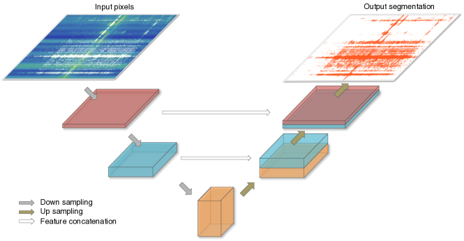
Instead of relying on a traditional architecture, the U-Net extends the contracting path of a CNN by a symmetric expansive path. As shown in Figure 1, the information on the extracted complex features (orange box) from the pooling path are propagated to the higher layers by several upsampling operations. The downsampling path followed by the upsampling path resembles a U-shape leading to the name of this network architecture.

We have reimplemented the original U-Net [20], written in Caffe, with the open source library Tensorflow following its exact architecture. Our Tensorflow U-Net implementation is written in Python with maximal flexibility in mind. The package is published on GitHub under GPLv3 license and can be used for various classification tasks (see A and B for installation instructions and usage examples). In the contracting path we apply in each layer two consecutive unpadded convolutions both followed by a rectifier linear unit (ReLU) activation and a $2\times 2$ max pooling downsampling operation. At each layer we double the number of extracted features. In the expansive path we replace the max pooling by an up-convolution that halves the number of features from the previous layer and concatenate the result with the features from the corresponding contraction layer. Finally, we apply a $1\times 1$ convolution to map the features from the last layer to the number of class labels i.e. to a binary decision if a pixel is contaminated or not. To obtain the probability of a pixel to belong to a certain class we convert the resulting output map with a pixel-wise soft-max layer. The RFI mitigation is done by inputting the TOD and applying a threshold on the predicted probability of each pixel to be contaminated with RFI.

2.2 Training the network

We train the parameters of the U-Net using the early Science Verification data acquired at the Bleien Observatory [2]. This data set was collected using a 7m single-dish telescope operating in drift-scan mode with a frequency range of 990 – 1260 MHz. We have processed the data with the HIDE & SEEK radio data processing pipelines described in [18]. The pipeline employs the SumThreshold algorithm to mask pixels contaminated with RFI. SumThreshold is a widely used iterative algorithm that is gradually building a mask to flag the unwanted signal. It follows the underlying assumption that the astronomical signal is relatively smooth, both, in time and frequency direction. While RFI signal exhibit patterns with sharp edges. The algorithm gradually improves a model of the astronomical signal and masks values lying above a certain threshold after subtracting this model from the data. It starts with localized, strong RFI bursts and extends the mask by gradually analyzing the neighboring pixels [18]. The parameters we adopt for the SumThreshold algorithm here are based on the procedure developed in [18]. We use the SumThreshold mask as ground truth to train the neural network as well as to evaluate the performance of the network on a separate test set. We note, however, that the RFI mask produced by SumThreshold is not perfect. It has a high false-positive-rate i.e. many pixels are incorrectly flagged as RFI. Some RFI detection pipelines have refined this technique, e.g. by using a scale invariant dilation operation[24]. This can improve the flagging performance of the algorithm. However, we demonstrate in this paper that our U-Net model is robust to this noise in the ground truth and is capable of correctly distinguishing between non-contaminated and contaminated pixels.

We explore the effects of various parameters on the classification performance and processing time. Here we report the effect of the parameters that most influence the performance such as the depth of the network (i.e. the number of layers), the number of features extracted in the first layer, and the size of the convolution kernels. We optimize a cross-entropy loss function to train the network parameters using a momentum-based stochastic gradient decent with an exponentially decaying learning rate with an initial value of 0.2. We initialize the weights of the network using a truncated normal distribution following the recommendation for the standard deviation in [20]. We train each network for 100 epochs each with a training mini-batch size of 32 on one TOD image with a resolution of $276\times 600$ pixels. For all configurations the loss function had reached a minima and remained stable. In order to avoid overfitting we use dropout layers [25] with a probability of 0.5 in all convolutions combined with an L2 regularizer of strength equal to $10^{-3}$. We train our networks using a NVIDIA Kepler K20 GPU.

3 Experimental results

To assess if a CNN can be used for the RFI mitigation task described in the previous section, we first apply our U-Net implementation to simulated radio data. We used the publicly available HIDE package to simulate radio data contaminated by RFI. The simulation used here reflect the drift-scan data of the early Science Verification survey taken at the Bleien Observatory. HIDE simulates the noise effects of the instrument and the atmosphere on the data. Furthermore, elevation-dependent signal variations, such as side-lobe ground-pickup are also taken into account. The RFI model employed in the package simulates a simple but well understood interference pattern. Each RFI burst is defined by the same profile. The amplitude and the rate of the burst is randomly sampled such that the expected data loss of the observation site is matched. [18, 2]. We have access to the perfect ground truth of this simulated data since we know for each pixel if it has been perturbed by simulated RFI. This simplified the training procedure and allowed us to better quantify the performance of the network. We find that our U-Net implementation performs very well in identifying RFI pixels. As shown in Figure 3 the U-Net achieves an Area-Under-the-Curve (AUC) score of $\sim$0.96 and $\sim$0.92 for the receiver operating characteristic (ROC) and the Precision-Recall curve respectively (black dashed line). The black stars denotes the performance of SEEK’s SumThreshold on the same simulated data set. We note that SEEK is achieving a comparable performance in the ROC metric but has a lower precision and recall than our U-Net. The U-Net achieves a maximum $F_{1}$ score of $\sim$0.85 compared to $\sim$0.75 for SEEK’s SumThreshold algorithm.

In a second stage, we use the CNN trained on simulations to mitigate RFI in data taken at the Bleien Observatory. As described in [18] the RFI simulation in HIDE is relatively simple. Therefore the trained U-Net struggled to detect long lasting broadband RFI signatures in real data, such as satellite emissions since they were not simulated in HIDE at all.

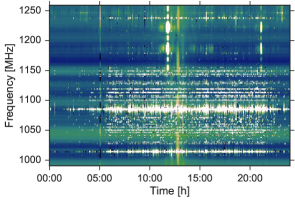
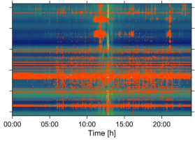
To achieve a better classification result on the observed data set we have processed the data with the SEEK data processing pipeline to obtain a RFI mask for the TOD derived from the SumThreshold algorithm. Compared to the perfect ground truth mask from the simulation, this SumThreshold mask contains incorrectly masked pixels and RFI pixels that were not detected. The left panel of Figure 2 shows an example of a set of rescaled, observed TOD used for the performance verification. We observe that the data is strongly contaminated by narrow and broadband RFI. For example, the extended burst between 1150 and 1250 MHz at around 11am can be attributed to a satellite passing through the telescope beam. The central panel displays the same dataset overlaid with SEEK’s SumThreshold mask. We find that the pipeline captures most of the RFI signal, but part of the uncontaminated data is incorrectly masked, e.g. in the range 1070 to 1100 MHz between 0 and 5am. The incorrect masking is mainly associated with the parameter setting of the mask dilation and smoothing. Defining these parameters is particularly challenging because the characteristics of the RFI in day time and night time are significantly different and its is hard for a single set of parameters to satisfy both. Here, for example, if we turn down the mask dilation to recover the clean data at night, the mask during the day will be sub-optimal

Figure 2: The left panel displays 24 hours of observed TOD from the Bleien Observatory. The broadband RFI contamination mainly comes from the nearby airport and is visible in the 1025–1150 MHz frequency band. The TOD also demonstrates the variation in the RFI level between day and night as the amount of RFI clearly increased at around 6:00 am and decreased at 11:00 pm. The central panel shows the same TOD overlaid (orange) with the RFI mask obtained from SEEK’s SumThreshold. The right panel displays the RFI mask from our U-Net with 3 layers and 64 features.

Figure 3: The left panel shows the receiver operating characteristic (ROC) curve for different U-Net configurations. The right panel depicts the precision-recall curve for the same architectures. The black dashed line shows the performance of the U-Net on simulated data sets while the other lines are showing the results on real data. The stars denote the performance of SEEK’s SumThreshold on the simulated data set.

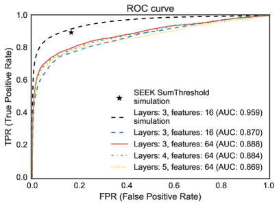
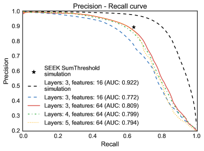
The left panel of Figure 3 shows the ROC curve for different U-Net configurations. The x-axis displays the ratio of pixels incorrectly labeled as RFI while the y-axis represents the ratio of correctly masked pixels. The right panel shows the precision-recall curve for the same network configurations. The black dashed lines show the performance for the network on simulated data. The other curves display the result on the observed data sets. The colored lines in these plots show that, beyond a certain network complexity, further increase in the number of layers or features does not significantly improve the performance of the network. We find that using a U-Net with 3 layers and 64 features (red solid line) provides a good balance in terms of prediction performance and computational cost. The network can be trained in a few hours on a modern GPU. The RFI detection throughput with this trained network is approximately 11.6 GB/h/GPU. The AUC score is lower on the observed than on the simulation data set as expected. This can be attributed to the increased complexity of the data and more importantly, the imperfect ground truth.

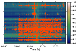
The right panel of Figure 2 shows the observed TOD overlaid with the mask obtained from our U-Net with 3 layers and 64 features. The CNN captures narrow and broadband RFI signatures very well such that the mask resembles SEEK’s SumThreshold output. The network has correctly learned the signatures of RFI signals such that it can compensate for the incorrectly masked pixel of the imperfect ground truth. Compared to the SumThreshold mask, we see that the power of the CNN approach is that it can automatically learn the local characteristics of the data in the time-frequency plane in a flexible and natural way.

4 Conclusion

Large surveys in the radio wavelength, especially of the 21cm neutral hydrogen line, is emerging as one of the most promising probes for cosmology. The resulting data will allow us to map out the structure of the Universe over a wide period of cosmic time and reveal parts of the Universe that is not accessible via other wavelengths. In the coming decades, we expect a very large amount of radio data to be collected and analyzed. One of the major challenges in processing radio data is the masking of radio frequency interference (RFI). The complex nature of RFI in both the time and frequency domain means that designing a general automated algorithm for RFI masking is a challenging task. The most popular existing method relies on thresholding algorithms, which require tuning of the threshold parameters. In some RFI masking pipelines this can be done automatically but for optimal performance further, manual tuning is typically necessary. The false-positive rate achieved by these algorithms often also depend on the RFI environment at the telescope.

In this paper, we presented a novel approach to RFI mitigation which makes use of recent advances in deep learning. We adopt a special architecture of a Convolutional Neural Network (CNN) that has proven to be very successful for various classification problems. This U-Net learns a set of features extracted from the input time-ordered-data (TOD) from a radio telescope in order to distinguish between the astronomical signal and the diverse and complex RFI signatures. Our U-Net is implemented with Google’s Tensorflow package and is capable of returning the probability for each pixel if it is contaminated with RFI. The code is made publicly available under GPLv3 license and can be used for diverse generic classification problems.

We have made use of the open source HIDE & SEEK radio data simulation and processing packages to train and assess the performance of our U-Net. We first trained the network on a simulated dataset where a perfect ground truth is available. We find that the U-Net achieves an excellent result, confirming the applicability of CNN to this problem. We then applied the same code on radio data taken at the Bleien Observatory. As no ground truth is available with the observed dataset, we processed the TOD with SEEK. SEEK’s SumThreshold RFI mitigation algorithm produced a RFI mask that we used as ground truth for training and performance measurement. The ground truth is however not perfect as it contains pixel that are incorrectly masked as RFI and some of the contaminated pixels were not flagged. We tested our U-Net with various different configurations on the same data set, and all of them perform reasonably well in the receiver operating characteristic (ROC) and precision-recall curve. Both measures however, are strongly, negatively biased as expected due to the imperfect ground truth. Visual inspection of the predicted RFI mask shows that this approach is showing competitive accuracy to classical RFI mitigation algorithms such as SEEK’s SumThreshold implementation.

This work is the first step in applying CNN to the RFI mitigation problem. Several improvements and extensions are possible to make the method even more powerful. For example, one can retrain the pre-trained network on a small data subset with an improved ground truth. In addition, one can imagine altering the loss function so that masking the astronomical signal of interest is penalized. In light of the large amount of radio survey data that will become available in the coming decades, applications of the CNN techniques on RFI masking can potentially be a promising alternative to other conventional techniques.

Appendix A Distribution

The package is released under the GPLv3 license and the development is coordinated on GitHub http://github.com/jakeret/tf_unet and contributions are welcome.

To be able to use the package you have to clone the repository and make sure you have Tensorflow correctly installed on your machine. All other project dependencies will be installed automatically during the setup procedure:

$ python setup.py develop --user

Appendix B Tensorflow U-Net usage example

Our Tensorflow U-Net implementation was written with flexibility in mind such that the package can be used for various classification problems. The typical use of our code looks like this:

from tf_unet import unet

net = unet.Unet(layers=3, features_root=64, channels=1, n_class=2)
trainer = unet.Trainer(net)
path = trainer.train(data_provider, output_path, training_iters=32, epochs=100)

After importing the package we create a Unet instance with 3 layers and 64 features. We use the network on grey-scaled images, hence we set channels to 1. For RGB-images for example the number of channels would be 3. The network should learn to predict a binary problem (e.g. pixel is RFI or not). Therefore we set the number of classes to 2. Next, we create a Trainer and train the network for 100 epochs with 32 training iterations. We pass an output path where the network and intermediate learning statistics should be stored, and a data_provider which can be a simple function or a callable that is providing data and labels for the training process. The code expects that the data has the shape [number of images, nx, ny, channels] for the data and [number of images, nx, ny, number of classes] for the one-hot encoded labels, where nx and ny denotes the size of the images in pixels.

To obtain a prediction form the network we perform:

prediction = net.predict(output_path, x_test)

We provide the path to the trained network on the file system and pass the data set on which we would like to run the network prediction. Both, the Unet and the Trainer implementation offer further parametrizations that are described in the package documentation.

References

- [1] J. R. Pritchard, A. Loeb, 21 cm cosmology in the 21st century, Reports on Progress in Physics 75 (8) (2012) 086901. arXiv:1109.6012, doi:10.1088/0034-4885/75/8/086901.
- [2] C. Chang, C. Monstein, J. Akeret, S. Seehars, A. Refregier, A. Amara, A. Glauser, B. Stuber, An integrated system at the bleien observatory for mapping the galaxy, arXiv preprint arXiv:1607.07451.
- [3] M. Van Haarlem, M. Wise, A. Gunst, G. Heald, J. McKean, J. Hessels, A. De Bruyn, R. Nijboer, J. Swinbank, R. Fallows, et al., Lofar: The low-frequency array, Astronomy & Astrophysics 556 (2013) A2.
- [4] G. Paciga, J. G. Albert, K. Bandura, T.-C. Chang, Y. Gupta, C. Hirata, J. Odegova, U.-L. Pen, J. B. Peterson, J. Roy, et al., A simulation-calibrated limit on the h i power spectrum from the gmrt epoch of reionization experiment, Monthly Notices of the Royal Astronomical Society (2013) stt753.
- [5] Z. S. Ali, A. R. Parsons, H. Zheng, J. C. Pober, A. Liu, J. E. Aguirre, R. F. Bradley, G. Bernardi, C. L. Carilli, C. Cheng, et al., Paper-64 constraints on reionization: The 21 cm power spectrum at z= 8.4, The Astrophysical Journal 809 (1) (2015) 61.
- [6] K. Bandura, G. E. Addison, M. Amiri, J. R. Bond, D. Campbell-Wilson, L. Connor, J.-F. Cliche, G. Davis, M. Deng, N. Denman, et al., Canadian hydrogen intensity mapping experiment (chime) pathfinder, in: SPIE Astronomical Telescopes+ Instrumentation, International Society for Optics and Photonics, 2014, pp. 914522–914522.
- [7] R. Battye, I. Browne, C. Dickinson, G. Heron, B. Maffei, A. Pourtsidou, H i intensity mapping: a single dish approach, Monthly Notices of the Royal Astronomical Society (2013) stt1082.
- [8] R. Battye, M. Brown, I. Browne, R. Davis, P. Dewdney, C. Dickinson, G. Heron, B. Maffei, A. Pourtsidou, P. Wilkinson, Bingo: a single dish approach to 21cm intensity mapping, arXiv preprint arXiv:1209.1041.
- [9] J. C. Pober, A. Liu, J. S. Dillon, J. E. Aguirre, J. D. Bowman, R. F. Bradley, C. L. Carilli, D. R. DeBoer, J. N. Hewitt, D. C. Jacobs, et al., What next-generation 21 cm power spectrum measurements can teach us about the epoch of reionization, The Astrophysical Journal 782 (2) (2014) 66.
- [10] X. Chen, The tianlai project: a 21cm cosmology experiment, in: International Journal of Modern Physics: Conference Series, Vol. 12, World Scientific, 2012, pp. 256–263.
- [11] G. Mellema, L. Koopmans, H. Shukla, K. K. Datta, A. Mesinger, S. Majumdar, et al., Hi tomographic imaging of the cosmic dawn and epoch of reionization with ska, arXiv preprint arXiv:1501.04203.
- [12] A. Offringa, A. de Bruyn, M. Biehl, S. Zaroubi, G. Bernardi, V. Pandey, Post-correlation radio frequency interference classification methods, Monthly Notices of the Royal Astronomical Society 405 (1) (2010) 155–167.
- [13] P. Fridman, W. Baan, mitigation methods in radio astronomy, Astronomy & Astrophysics 378 (1) (2001) 327–344.
- [14] J. Zhao, X. Zou, F. Weng, Windsat radio-frequency interference signature and its identification over greenland and antarctic, IEEE Transactions on Geoscience and Remote Sensing 51 (9) (2013) 4830–4839.
- [15] W. Baan, P. Fridman, R. Millenaar, Radio frequency interference mitigation at the westerbork synthesis radio telescope: Algorithms, test observations, and system implementation, The Astronomical Journal 128 (2) (2004) 933.
- [16] A. Offringa, A. de Bruyn, S. Zaroubi, M. Biehl, A lofar rfi detection pipeline and its first results, arXiv preprint arXiv:1007.2089.
- [17] L. W. Peck, D. M. Fenech, Serpent: Automated reduction and rfi-mitigation software for e-merlin, Astronomy and Computing 2 (2013) 54–66.
- [18] J. Akeret, S. Seehars, C. Chang, C. Monstein, A. Amara, A. Refregier, Hide & seek: End-to-end packages to simulate and process radio survey data, arXiv preprint arXiv:1607.07443.
- [19] C. J. Wolfaardt, Machine learning approach to radio frequency interference (rfi) classification in radio astronomy, Ph.D. thesis, Stellenbosch University (2016).
- [20] O. Ronneberger, P. Fischer, T. Brox, U-net: Convolutional networks for biomedical image segmentation, in: International Conference on Medical Image Computing and Computer-Assisted Intervention, Springer, 2015, pp. 234–241.
- [21] R. Collobert, J. Weston, L. Bottou, M. Karlen, K. Kavukcuoglu, P. Kuksa, Natural language processing (almost) from scratch, Journal of Machine Learning Research 12 (Aug) (2011) 2493–2537.
- [22] A. Krizhevsky, I. Sutskever, G. E. Hinton, Imagenet classification with deep convolutional neural networks, in: Advances in neural information processing systems, 2012, pp. 1097–1105.
- [23] R. Collobert, J. Weston, A unified architecture for natural language processing: Deep neural networks with multitask learning, in: Proceedings of the 25th international conference on Machine learning, ACM, 2008, pp. 160–167.
- [24] A. Offringa, J. Van de Gronde, J. Roerdink, A morphological algorithm for improving radio-frequency interference detection, Astronomy & Astrophysics 539 (2012) A95.
- [25] N. Srivastava, G. E. Hinton, A. Krizhevsky, I. Sutskever, R. Salakhutdinov, Dropout: a simple way to prevent neural networks from overfitting., Journal of Machine Learning Research 15 (1) (2014) 1929–1958.