Deep Reinforcement Learning for Tensegrity Robot Locomotion

Abstract

Tensegrity robots, composed of rigid rods connected by elastic cables, have a number of unique properties that make them appealing for use as planetary exploration rovers. However, control of tensegrity robots remains a difficult problem due to their unusual structures and complex dynamics. In this work, we show how locomotion gaits can be learned automatically using a novel extension of mirror descent guided policy search (MDGPS) applied to periodic locomotion movements, and we demonstrate the effectiveness of our approach on tensegrity robot locomotion. We evaluate our method with real-world and simulated experiments on the SUPERball tensegrity robot, showing that the learned policies generalize to changes in system parameters, unreliable sensor measurements, and variation in environmental conditions, including varied terrains and a range of different gravities. Our experiments demonstrate that our method not only learns fast, power-efficient feedback policies for rolling gaits, but that these policies can succeed with only the limited onboard sensing provided by SUPERball’s accelerometers. We compare the learned feedback policies to learned open-loop policies and hand-engineered controllers, and demonstrate that the learned policy enables the first continuous, reliable locomotion gait for the real SUPERball robot. Our code and other supplementary materials are available from http://rll.berkeley.edu/drl_tensegrity

I Introduction

Tensegrity robots are a class of robots that are composed of rigid rods connected through a network of elastic cables. These robots are lightweight, low cost, and capable of withstanding significant impacts by deforming and distributing force across the entire structure. These properties make them a promising option for future planetary exploration missions, as their compliance protects the robot and its payload during high-speed descent and landing, and may also allow for greater mobility and robustness during exploration of rugged and dangerous environments [1].

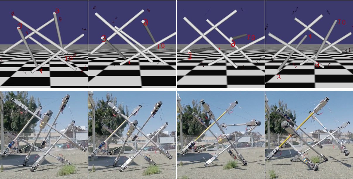
Figure 1: Left to right: a rolling motion toward the camera performed by the SUPERball simulation (top) and the physical SUPERball robot (bottom). The rolling gait is learned from scratch in simulation with our proposed algorithm, and uses only the onboard accelerometer sensors for feedback.

However, efficient locomotion for tensegrity robots is a challenging problem. Such robots are typically controlled through actuation of motors that extend and contract their cables, thereby changing their overall shape. Many such systems are underactuated because there are usually more cables than motors. Furthermore, actuating one motor can change the entire shape of the robot, leading to complex, highly coupled dynamics. As such, hand-engineering locomotion controllers is unintuitive and time-consuming and, as our experimental results in Section VI show, such controllers often do not generalize well to different environments. In particular, since the goal of these robots involves deployment to celestial bodies with vastly different terrains, gravities, and compositions, it is preferable to have policies be automatically generated for each environment rather than to independently hand-engineer controllers for each setting. This motivates using learning algorithms to automatically discover successful and efficient behavior.

Robotic learning methods have previously produced successful policies for tasks such as locomotion for bipeds and quadrupeds [2, 3, 4, 5, 6, 7]. These methods, however, typically require hand-engineered policy classes, such as a linear function approximator using a set of hand-designed features as input [2]. For many tensegrity systems, it is difficult to design suitable policy classes, since the structure of a successful locomotion strategy might be highly complex. We illustrate this in Section VI, by demonstrating that it is desirable to have a representation that is closed-loop, since open-loop control, though simpler to design and implement, does not generalize as well to changes in terrain, gravity, and other environmental and robot parameters.

Some more recent methods learn deep neural network policies that are successful for tasks such as grasping with robotic arms and bipedal locomotion [8, 9], and such policies are more expressive and require less hand-engineering compared to policy classes used in previous methods. One such method, which we extend in this work, is mirror descent guided policy search (MDGPS), a recently developed algorithm that frames the guided policy search (GPS) alternating optimization framework as approximate mirror descent [10]. We choose MDGPS in our work because it allows us to learn deep neural network policies while maintaining sample efficiency, and it presents a natural extension to periodic locomotion tasks which we describe in Section IV.

A key problem for locomotion tasks is the difficulty of establishing stable periodic gaits, and this is exacerbated for tensegrity robots due to their complex dynamics and unusual control mechanisms. As shown in our experiments, near-stable behavior with even small inaccuracies can lead to compounding errors over time, and will not be successful in producing a continuous periodic gait. Previous algorithms have dealt with this problem by establishing periodicity directly through the choice of policy class [3, 11, 12], utilizing a large number of samples [8], or initializing from demonstrations [13, 14]. Instead, we handle this challenge by sequentially training several simple policies that demonstrate good behavior from a wide range of states, and then learning a policy that reproduces the gait of all of the sequential policies for a successful periodic behavior. The resulting algorithm learns a policy from scratch for locomotion of a tensegrity robot, a task that exhibits periodicity over long time horizons. We demonstrate through our experiments that this learned policy is capable of efficient, continuous locomotion in a range of different conditions by learning appropriate feedbacks from the robot’s onboard sensors.

The main contribution of this paper is a method for automatically learning locomotion policies represented by general-purpose neural networks, which we demonstrate by learning a gait for the Spherical Underactuated Planetary Exploration Robot ball (SUPERball), the tensegrity robot shown rolling in Figure 1. To this end, we extend the MDGPS algorithm so as to make it suitable for learning long, periodic gaits, by training groups of sequential policies as supervision for learning a successful neural network policy. Our experimental results show that our method learns efficient rolling behavior for SUPERball both in simulation and on the real physical robot. We make comparisons between the learned policies and two open-loop representations, one learned and one hand-engineered, to demonstrate the benefits of learning and feedback for fast and reliable locomotion.

II Related Work

Early work in tensegrity research was focused on modeling the statics of tensegrity structures [15, 16, 17]. This led to the development of kinematic controllers which enable quasi-static locomotion [18]. More recent work has developed dynamic locomotion controllers [19] in simulation using the NASA Tensegrity Robotics Toolkit (NTRT) [20]. Iscen et al. used coevolutionary learning that exploited the symmetry of a simulated SUPERball-like robot to learn an efficient rolling controller [21]. This controller required 24 actuators on the robot, which does not match the current robot’s 12 actuators. We also do not exploit the symmetry of SUPERball as this strategy is less reliable on the real robot. A snake-like tensegrity robot learned different locomotion gaits which utilized Central Pattern Generators [22], which were then managed by a neural network to achieve goal directed behavior over various terrains. However, they utilized Monte Carlo simulation techniques requiring thousands of trials to learn their policies. This makes it impractical to learn on real hardware. Mirletz et al. successfully transferred a learned policy to a real robotic prototype [23], but the policy parameters required hand-tuning.

Previous work in robotic locomotion has produced successful bipedal locomotion using passive-dynamic walkers [24] and virtual model control [25], as well as spring-mass running based on biological models [26]. However, these works used analytic models built through human insight and simplified models, and are therefore difficult to generalize to radically different systems such as tensegrities. Robotic learning methods have successfully learned locomotion policies for bipeds [2, 11, 12] and quadrupeds [3]. These methods require careful consideration and design of the policy class, which typically have fewer than 100 parameters [27]. More recent work in deep reinforcement learning has learned deep neural network policies for bipedal running [8] and 2D systems such as swimmers and hoppers [13, 14]. These methods, however, typically require a large number of samples corresponding to weeks of training time [8], or initialize from demonstrations [13, 14].

Several methods have been proposed for the direct transfer of policies learned in simulation to the real world. Cutler et al. used a transition from simple to complex simulations, which are assumed to increase in both cost and fidelity to the real-world setting, to reduce the amount of training time needed in the real world [28]. Mordatch et al. optimized trajectories through an ensemble of models perturbed with noise to find trajectories that could be successfully transferred to the real world setting [29]. Our approach also introduces noise into the simulation, and we found that this can help in training policies that are successful in a wide range of simulated terrain and gravity settings.

III Background

In this section, we present background on tensegrity robots, as well as policy search methods. In particular, we describe the MDGPS algorithm [10], which we extend in this work to optimize periodic locomotion gaits.

III-A Tensegrity Robotics

Tensegrity (tensile-integrity) structures are free-standing structures with axially loaded compression elements in a network of tension elements. Ideally, each element of the structure experiences either pure axial compression or pure tension [30, 31]. The absence of bending or shear forces allows for highly efficient use of materials, resulting in lightweight yet robust systems. Because the rods are not directly connected, tensegrities have the unique property that externally applied forces distribute through the structure via multiple load paths. This property creates a soft robot out of inherently rigid materials. Since there are no rigid connections within the structure, there are also no lever arms to magnify forces. The result is a global level of robustness and tolerance to forces applied from any direction.

The SUPERball tensegrity robot, shown in Figure 2, is designed to explore a new class of planetary exploration robot which is able to deploy from a compact launch volume, land at high speeds without the use of air-bags, and provide robust surface mobility [1, 32]. SUPERball is made up of six identical rods suspended together by 24 cables to form an icosahedron geometry. The cables have a linear spring attached in-line, giving the system series elasticity and compliance. Each rod of SUPERball is comprised of two modular robotic platforms (end caps), as defined in [1]. Each end cap is equipped with an inertial measurement unit (IMU), a motor with encoder, and a control board. Since there is only one motor per end cap, SUPERball can only actuate 12 of its 24 cables, and this by definition makes the system underactuated. A basic locomotion strategy for SUPERball is to contract a cable that is a part of the current ground face of the robot, thus shrinking the triangle base and causing the robot to tip over [1]. More sophisticated locomotion may still follow this strategy, but may also utilize other cables to allow for greater efficiency in transitioning to the next ground face. These sophisticated strategies are difficult to hand-engineer, but we demonstrate that they can be learned using policy search algorithms such as MDGPS.

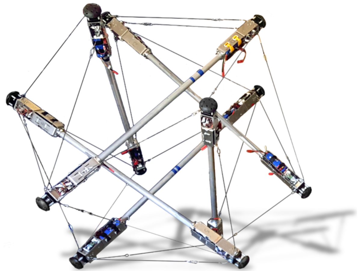
Figure 2: The SUPERball tensegrity robot. This robot is composed of six identical rods and 24 cables, 12 of which can be actuated using the motors connected to the ends of each rod. This work uses the onboard IMUs and motor encoders on each of the end caps.

III-B Mirror Descent Guided Policy Search

Figure 3: Diagram of the MDGPS algorithm described in Algorithm 1. As described in Section IV, our approach differs from standard MDGPS in the highlighted box at the top. The choice of whether to collect samples from the local policies $p_{i}$ or global policy $\pi_{\theta}$ is a hyperparameter.

Policy search algorithms aim to find a good policy by directly searching through the space of policy parameters. Formally, we wish to find a setting of the policy parameters $\theta$ to optimize the policy $\pi_{\theta}(\mathbf{u}_{t}|\mathbf{o}_{t})$ with respect to the expected cost. In the finite-horizon episodic setting, the expected cost under the policy is given by $J(\theta)=\sum_{t=1}^{T}\mathbb{E}_{\pi_{\theta}}[\ell(\mathbf{x}_{t},\mathbf{u}_{t})]$, where $\ell(\mathbf{x}_{t},\mathbf{u}_{t})$ is the cost function. Here $\mathbf{x}_{t}$ denotes the state of our system at time $t$, $\mathbf{o}_{t}$ denotes the observation of the state, and $\mathbf{u}_{t}$ denotes the action.

Guided policy search algorithms use supervised learning to train the policy, with supervision coming from several local policies $p_{i}(\mathbf{u}_{t}|\mathbf{x}_{t})$ that are optimized to succeed only from a specific initial state of the task, using full state information. This is much simpler than the goal of the global policy, which is to succeed under partial observability from any initial condition sampled from the initial state distribution. These simplifications allow the use of simple and efficient methods for training the local policies, such as trajectory optimization methods when there is a known model, or trajectory-centric reinforcement learning (RL) methods [14]. The specific algorithm used in this work is MDGPS, which interprets GPS as approximate mirror descent on $J(\theta)$ [10]. The local policies are optimized to minimize $J(\theta)$ subject to a bound on the KL-divergence between the local policy $p_{i}$ and the global policy $\bar{\pi}_{\theta{i}}$, following previous work [33, 34, 35, 8]. Optimizing the global policy is done using the samples collected in the current iteration, which are used in a supervised fashion to approximately minimize the divergence between the global policy and the local policies.

Algorithm 1 Mirror descent guided policy search (MDGPS)

1:  for iteration $k=1$ to $K$ do

2:     Run either each $p_{i}$ or $\pi_{\theta}$ to generate episodes $\{\tau\}$

3:     Set $p_{i}\leftarrow\operatorname*{arg\,min}_{\hat{p}_{i}}\mathbb{E}_{\hat{p}_{i}}[\ell(\tau)]~{}s.t.~{}D_{KL}(\hat{p}_{i}\|\pi_{\theta{i}})\leq\epsilon$

4:     Train $\pi_{\theta}$ using supervised learning on $\{\tau\}$

5:  end for

The generic MDGPS algorithm is summarized in Algorithm 1 and depicted in Figure 3. In the top box, corresponding to line 2, samples are collected by running either the global policy or the local policies. This choice between “on-policy” and “off-policy” sampling is set by the user, and previous work has noted that “on-policy” sampling aids in the generalization capabilities of the final policy [10]. In the center and bottom boxes, corresponding to line 3, the algorithm improves the local policies using an LQR-based update: the samples are first used to fit time-varying linear dynamics for each local policy, and these fitted dynamics are then used with a KL-constrained LQR optimization to update the linear-Gaussian local policies. This corresponds to a simple model-based trajectory-centric RL method, and further details can be found in prior work [14]. In the right box and on line 4, the global policy $\pi_{\theta}(\mathbf{u}_{t}|\mathbf{x}_{t})$ is updated using supervised learning, with the training data corresponding to the observations along the episodes, with actions given by the updated local policies. This causes the global policy to “catch up” to the local policies, improving its behavior for the next iteration.

IV Optimizing Periodic Gaits with MDGPS

The efficiency and speed of model-based policy optimization methods, such as the LQR-based method used to optimize the local policies in MDGPS, is due in large part to the fact that dynamic programming can allow for large changes to a policy that would be impractical with purely sample-based model-free methods [14]. However, in complex stochastic domains, such as the contact-rich dynamical system of a rolling tensegrity robot, the accumulation of uncertainty and variability under an unstable policy and compounding modeling errors can make it difficult to apply dynamic programming over the long horizons needed to establish a periodic gait. Specifically, the LQR-based update we use fits a time-varying linear-Gaussian dynamics model $p(\mathbf{x}_{t+1}|\mathbf{x}_{t},\mathbf{u}_{t})=\mathcal{N}(f_{\mathbf{x}t}\mathbf{x}_{t}+f_{\mathbf{u}t}\mathbf{u}_{t},\mathbf{F}_{t})$ and simulating this model forward becomes increasingly inaccurate with the system complexity and the length of the horizon.

We demonstrate this effect through our experimental results in Section VI-B and in the appendix. In this section, we describe how we can obtain a policy with stable periodic behavior by first splitting the task across multiple policies, each optimized over a smaller time segment where it is easier to apply dynamic programming, and establishing good behavior across the range of states visited by these policies. Following the framework of GPS algorithms, we subsequently learn a global policy that can generalize the behavior of the local policies and encapsulate a successful periodic gait.

GPS algorithms such as MDGPS use supervised learning to learn a global policy, where the supervision comes from several local policies $p_{i}(\mathbf{u}_{t}|\mathbf{x}_{t})$, $i\in\{1,\ldots,C\}$. Each local policy is trained from a different initial state, where $C$ is the chosen number of initial states. Each local policy is optimized over $T^{p}$ time steps, and we wish to learn a global policy $\pi_{\theta}(\mathbf{u}_{t}|\mathbf{o}_{t})$ that can succeed by generalizing the behavior of these local policies over an episode of length $T^{\pi}$. In manipulation tasks, we usually set $T^{\pi}=T^{p}$, depending on the horizon that we want the task to be accomplished by [36]. In locomotion tasks, we ideally want the global policy to exhibit continuous successful behavior, i.e., $T^{\pi}=\infty$, and we can empirically determine $T^{p}$ based on the amount of supervision the global policy needs to learn a continuous periodic gait. In our work, we simply initialize $T^{p}$ to a short horizon, and, should this fail, we restart the experiment with an increased $T^{p}$. We repeat this process until the global policy learns a successful locomotion gait.

If the required $T^{p}$ is long, as is the case for the SUPERball locomotion task, it is difficult to optimize a local policy over this time horizon due to the accumulation of uncertainty and errors described earlier. In our method, we instead learn $L$ local policies $p_{i}^{1},\ldots,p_{i}^{L}$ for each initial state $i$, each optimized for $T^{p}/L$ time steps. For the local policies $p_{i}^{j}$, $j\in\{2,\ldots,L\}$, we set the initial state $\mathbf{x}_{0}^{j}$ to be the final state of the preceding local policy, i.e., $\mathbf{x}_{T^{p}/L}^{j-1}$. This amounts to training local policies in a sequential fashion, where the $L$ local policies together are optimized over $T^{p}$ time steps. In practice, we found that the variance of $\mathbf{x}_{T^{p}/L}^{j-1}$ is too high at the beginning of training for $p_{i}^{j}$ to be successful, so we train $p_{i}^{j-1}$ until it stabilizes before starting to train $p_{i}^{j}$.

In previous work, the motivation behind choosing multiple initial states was so that the global policy could succeed from all of these initial states, and ideally generalize to other initial states as well [36]. In our work, we found that choosing multiple initial states is also beneficial in learning a stable periodic gait compared to having just one initial state, and Section VI-B demonstrates this difference. The reason for this is that, to achieve the same amount of supervision using only one initial state, the sequence of local policies $p_{1}^{1},\ldots,p_{1}^{L}$ must be much longer, and training a longer sequence increases the chances of divergence and instability in the behavior of the local policies, due to compounding variance in the starting states of later policies, compared to training shorter sequences from several stable initial states.

Algorithm 2 MDGPS with sequential local policies

1:  for iteration $k=1$ to $K$ do

2:     for $i=1$ to $C$ do

3:        $S_{i}\leftarrow\{\}$

4:        for the desired number of episodes do

5:           $x_{0}\leftarrow$ initial state $i$

6:           for $l=1$ to $L$ do

7:              Run either $p_{i}^{l}$ or $\pi_{\theta}$ to generate episode $\tau$

8:              $S_{i}\leftarrow{S_{i}}\cup\{\tau\}$

9:              $x_{0}\leftarrow$ end state of $\tau$

10:           end for

11:        end for

12:        for $l=1$ to $L$ do

13:           $p_{i}^{l}\leftarrow\operatorname*{arg\,min}_{\hat{p}_{i}^{l}}\mathbb{E}_{\hat{p}_{i}^{l}}[\ell(\tau)]~{}s.t.~{}D_{KL}(\hat{p}_{i}^{l}\|\pi_{\theta{i}})\leq\epsilon$

14:        end for

15:     end for

16:     Train $\pi_{\theta}$ using supervised learning on $\bigcup_{i}S_{i}$

17:  end for

Our method is detailed in Algorithm 2. On line 7, we collect samples from either the local policies or global policy. In our work, we start by sampling from the local policies, and we switch to sampling from the global policy after a fixed number of iterations, which we set empirically based on the performance and stability of the local policies. This allows for the local policies to establish good rolling behavior at the beginning, and then for the global policy to generalize this into continuous rolling. On line 8, we store the collected episode, and in order to run the policies sequentially, we set the starting state of the next policy to be the end state of the episode $\tau$ collected from the current policy. The rest of the algorithm is identical to standard MDGPS – note that lines 3 through 11, 12 through 14, and 16 in Algorithm 2 correspond to line 2, 3, and 4, respectively, in Algorithm 1.

V Learning Locomotion for SUPERball

For SUPERball locomotion, we chose six initial states that correspond to the robot resting on each of its stable ground faces. We set $T^{p}=100$ and $L=2$, so from each initial state $i$, two local policies $p_{i}^{1}$ and $p_{i}^{2}$ are optimized over 50 time steps each, where each time step is $0.1\text{\,}\mathrm{s}$. We found that a fully optimized local policy can perform about two transitions from one ground face to the next face over $5\text{\,}\mathrm{s}$. We also found it helpful in our work to not begin training $p_{i}^{2}$ until $p_{i}^{1}$ trains for several iterations, so that $\mathbf{x}_{50}^{1}$, which is $\mathbf{x}_{0}^{2}$, is more stable and has lower variance. We show in the appendix that training two local policies in this fashion is much more sample efficient than training one local policy for $10\text{\,}\mathrm{s}$, and produces smoother and faster rolling behavior. In total, in our work, 12 local policies are trained in sequences of two, and this provided the global policy the supervision required to learn to roll continuously.

V-A Kinematic Constraints for Safe Actions

One of the challenges with automated policy learning is that all requirements for the policy are generally encoded in the cost function, including task-level objectives such as desired rolling direction and hard constraints such as safety. Due to the structure of tensegrity systems, unsafe actuation of the motors can place the robot into configurations with unacceptable risk of cable or motor failure. The configurations associated with such high-tension conditions are difficult to encode analytically and even more difficult to balance against primary task objectives in the cost function. We therefore adopt a simple safety constraint approach to enable safe learning and policy execution on the SUPERball hardware. This approach is challenging to use with hand-engineered policies, which often exploit unsafe but effective actions to quickly yield a locomotion gait. However, the approach is much easier to adopt with learned policies, as it naturally embeds itself into the training procedure.

Specifically, we estimate the cable tensions for a particular set of actuator positions using a simple forward kinematics model of SUPERball. We repeat this process for many different randomly generated motor settings and store all sets of motor positions for which all cable tensions of the robot are below the acceptable threshold. Then, when the policy outputs an action, we use the Fast Library for Approximate Nearest Neighbors (FLANN) [37] to compute and command the nearest ($\ell_{1}$ norm) safe action. Computing the cable tensions for a given set of motor positions takes a few milliseconds using forward kinematics. As this is easily parallelized, we constructed a database containing about 100 million motor positions deemed safe in a few hours. At runtime, finding the nearest neighbor action takes roughly $200\text{\,}\mathrm{\SIUnitSymbolMicro s}$ and is easily embedded into both training and testing without disrupting the command frequency of $10\text{\,}\mathrm{Hz}$.

By separating this safety constraint from the cost function, we avoid the need to tune the parameters of the cost function to weigh the opposing objectives of speed and hardware safety. Furthermore, we encode safety as a hard constraint using this method, and we directly prevent unsafe actions rather than just penalizing them. Utilizing these kinematic constraints is extremely helpful in transferring policies learned in simulation directly onto the real robot. In simulation, the physical limits are less restrictive, and going beyond the safe limits does not have any adverse effects, so it is possible to train a policy that exploits these inaccuracies in order to succeed. We can make sure this does not happen by enforcing stronger constraints on what actions the policy can output, and it is more likely that the policy trained with these constraints in simulation will not fail on the real robot, or even worse, cause damage and hardware problems.

VI Experimental Results

In our experiments, we aim to answer several questions. First, can we learn policies in simulation that allow the simulated SUPERball to roll efficiently under various settings of terrain, gravity, sensor noise, and robot parameters? Second, do our learned feedback policies generalize better to changes in environmental and robot parameters compared to open-loop learned policies and hand-engineered controllers? Finally, can we transfer the learned policy from simulation to the real robot, and have the real robot roll?

Section VI-A details our experimental setup. In Section VI-B, we test in simulation the efficiency of the learned policies and make comparisons to establish the importance of learning and feedback. In Section VI-C, we evaluate a learned policy on the real robot. The appendix includes an additional experiment that illustrates the benefit of learning sequential policies, each over shorter time horizons.

VI-A Experimental Setup

We encode the state of the system $\mathbf{x}_{t}$ as the position and velocity of each of the 12 bar endpoints of SUPERball, and the position and velocity of each of the 12 motors, measured in radians, for a total dimensionality of 96. We experimented with two different representations for the observation $\mathbf{o}_{t}$. The “full” 36-dimensional observation includes motor positions, and also uses elevation and rotation angles and angular velocities calculated from the robot’s accelerometers and magnetometers. The “limited” observation is 12-dimensional and only uses the acceleration measurement along the bar axis from each of the accelerometers. We found that interfering magnetic fields near the testing grounds at NASA Ames cause the magnetometers to be unreliable and difficult to calibrate, and because of this, the policy using the limited observation is much easier to transfer on to the real robot. The action $\mathbf{u}_{t}$ is the instantaneous desired position of each motor, which may not be reached if the position is far away.

Each local policy required about 200 episodes before it was reliably successful. Simultaneously during training of the local policies, we learn a global policy, which in our work is a deep neural network with three hidden layers of 64 rectified linear units (ReLU) each, using the same samples. Our cost function $l(\mathbf{x}_{t},\mathbf{u}_{t})$ is simply the negative average velocity of the bar endpoints of the robot, which corresponds to the linear velocity of the center of mass. The local policies are therefore trained to roll as quickly as possible.

For completeness, the entire learning process took approximately $2\text{\,}\mathrm{h}$ on a CUDA-enabled quad-core Intel i7 computer utilizing $4\text{\,}\mathrm{GiB}$ of system memory. This is with each simulation set running at faster than real time and with the kinematic constraints mentioned in Section V-A. Without CUDA, the learning process takes approximately 20% longer.

VI-B Results in Simulation

		Our Method			Open-Loop
		Full Observation,	Limited Observation,	Limited Observation,	Mean Actions from	Hand-Engineered
		Six Initial States	Six Initial States	One Initial State	Best Learned Policy	Punctuated Rolling
Normal Conditions		$\mathbf{25.307\pm 0.309}$	$24.141\pm 0.352$	$20.008\pm 0.871$	$\mathit{25.076\pm 0.078}$	$10.266\pm 0.071$
[HTML]D3D3D3 [HTML]D3D3D3	[HTML]D3D3D3Hilly	[HTML]D3D3D3$\mathit{6.025\pm 2.835}$	[HTML]D3D3D3$\mathbf{9.568\pm 5.197}$	[HTML]D3D3D3$3.124\pm 1.083$	[HTML]D3D3D3$3.069\pm 2.201$	$1.734\pm 0.411$
[HTML]D3D3D3 [HTML]D3D3D3	[HTML]D3D3D3Uphill	[HTML]D3D3D3$\mathbf{18.547\pm 0.231}$	[HTML]D3D3D3$\mathit{16.107\pm 0.809}$	[HTML]D3D3D3$13.573\pm 0.174$	[HTML]D3D3D3$7.721\pm 0.236$	$8.136\pm 0.026$
[HTML]D3D3D3 [HTML]D3D3D3Terrain	[HTML]D3D3D3Downhill	[HTML]D3D3D3$\mathbf{32.896\pm 0.275}$	[HTML]D3D3D3$\mathit{29.970\pm 0.858}$	[HTML]D3D3D3$21.963\pm 2.403$	[HTML]D3D3D3$27.661\pm 0.136$	$11.264\pm 0.091$
	10%	$\mathbf{19.505\pm 0.746}$	$0.804\pm 0.103$	$0.776\pm 0.025$	$\mathit{18.024\pm 2.356}$	$11.044\pm 0.054$
	50%	$\mathbf{23.331\pm 0.871}$	$9.671\pm 0.550$	$0.996\pm 0.007$	$\mathit{19.673\pm 3.244}$	$10.310\pm 0.010$
Gravity	200%	$\mathit{27.600\pm 2.307}$	$\mathbf{30.095\pm 1.055}$	$16.422\pm 4.068$	$24.865\pm 0.190$	$9.845\pm 0.009$
[HTML]D3D3D3 [HTML]D3D3D3	[HTML]D3D3D3Heavy	[HTML]D3D3D3$12.521\pm 1.710$	[HTML]D3D3D3$\mathbf{14.561\pm 0.079}$	[HTML]D3D3D3$\mathit{12.972\pm 0.110}$	[HTML]D3D3D3$1.081\pm 0.019$	$10.550\pm 0.003$
[HTML]D3D3D3 [HTML]D3D3D3Robot	[HTML]D3D3D3End Cap Failure	[HTML]D3D3D3$\mathbf{23.215\pm 2.927}$	[HTML]D3D3D3$\mathit{21.595\pm 0.253}$	[HTML]D3D3D3$19.144\pm 0.207$	[HTML]D3D3D3$17.901\pm 1.967$	$10.222\pm 0.013$
	0%	$\mathbf{27.250\pm 0.203}$	$\mathit{25.798\pm 0.200}$	$20.918\pm 0.213$
Added Noise	20%	$8.739\pm 7.031$	$\mathbf{18.095\pm 0.406}$	$\mathit{17.613\pm 0.400}$	N/A	N/A

TABLE I: Average distances in meters traveled in simulation using the policies learned through our method with varying observation representations and local policy training schemes, the open-loop mean actions from the learned policy that performs best under training conditions, and the hand-engineered open-loop policy. Results are averaged across five trials of one minute each for a variety of terrain, gravity, noise, and robot settings. “Normal Conditions” are the training conditions, which are flat terrain, 100% gravity, 10% added noise to the input, and normal robot parameters. For the terrain settings, the hilly terrain contained hills that were $0.1\text{\,}\mathrm{m}$ tall, and the uphill and downhill terrains had slopes of $0.1\text{\,}\mathrm{rad}$. When varying one setting, all other settings remain the same as during training time. We do not test the open-loop controllers with varying input noise, because these controllers do not have any input. Bolded numbers indicate the farthest distance traveled for any given condition, and italicized numbers are the second farthest. Note that the first two learned policies generally outperform all other controllers, demonstrating the benefits of our method combined with multiple initial states.

The SUPERball simulation that we use is built off of the NTRT open-source project. Aside from speed and efficiency benefits, the simulation also allows us to systematically and easily vary the parameters of the robot and environment.

Our results for testing the learned policies against a range of environmental and robot parameters are presented in Table I. We report the average distance traveled over five trials of $60\text{\,}\mathrm{s}$ for three policies learned with MDGPS, an open-loop policy that outputs the mean actions from the learned policy that performs best under training conditions, and an open-loop hand-engineered controller. The policies learned with MDGPS use either the 36-dimensional observation or the 12-dimensional observation. To demonstrate the benefit of multiple initial states, we also learn a policy using the accelerometer observation and a long sequence of local policies, still trained over $5\text{\,}\mathrm{s}$ each, from one initial state. The open-loop hand-engineered controller is designed to follow the basic locomotion strategy described in Section III-A.

We systematically vary a suite of settings in simulation: the ground terrain, which can be flat, uneven, or sloped up or downhill; the strength of the gravitational field, which can be 10%, 50%, 100%, or 200% of Earth’s gravity; the noise level on the inputs to the policy, which can be 0%, 10%, and 20%; and various parameters of the robot. The noise we incorporate into the robot’s sensor readings includes Gaussian noise, with variance for each sensor type proportional to the range of the sensor, and randomly dropped sensor readings. Details about this noise can be found in the appendix. For robot parameters, we increase the mass of the rods and decrease the maximum motor velocities to create a heavier robot, and we simulate the failure of a specific end cap by dropping all sensors readings and motor commands.

The learned policy with full observation performs best under training conditions, and also demonstrates the best generalization across terrain and gravity settings as well as the noiseless condition. The learned policy with limited observation, though slightly slower than the policy with full observation, adapts better to the heavier robot as well as to motor failure, and also performs significantly better under heavy noise. These conditions are important for successful transfer to the real world setting, since the parameters of the physical SUPERball robot naturally differ from the simulation, and the imperfections in the hardware result in sensor and motor unreliability. The learned policy from the single long sequence of local policies does not perform as well as the other learned policies, because it is prone to diverge and become unstable, at which point it fails. In training this policy, we were unable to successfully train the fifth local policy to continue the gait, due to both the build-up in variance in the starting states of the local policies and the divergence in the behavior of the local policies from the desired periodic gait. The global policy learns a gait from the first four local policies, but the resulting behavior is less efficient and also significantly less stable.

The open-loop mean actions from the learned policy demonstrate comparable results under the training conditions, as expected, but its performance falls off drastically for most of the other conditions. Because a controller for SUPERball would ideally work under different terrains and in the presence of hardware issues, this shows that it is imperative that we use a closed-loop representation to ensure successful and reliable locomotion. The hand-engineered open-loop controller rolls consistently across most conditions, but is significantly slower than the three other policies. This emphasizes the benefits of learning and the difficulty in hand-engineering good controllers, as this controller was carefully designed but still sacrifices speed and other important benefits, such as robot safety, for reliability. Most notably, this hand-engineered controller has caused cable and motor failure on the physical SUPERball robot in the past, which is why we did not compare against it for the real robot results.

In summary, these results show that all learned policies substantially outperform the hand-engineered rolling controller, and the closed-loop neural network policies outperform the open-loop baselines in almost all conditions, indicating the benefits of both learning and feedback in SUPERball locomotion. Our method is able to learn successful and efficient policies even with the limited sensory observations provided by only SUPERball’s accelerometers, and the learned policies demonstrate generalization to unseen conditions representative of what a planetary exploration rover might encounter, such as changing terrains, unstable levels of noise, and hardware failure. The addition of input noise during training encourages this generalization, and results in learned policies with similar levels of reliability as the hand-engineered controller, though significantly faster and less likely to cause hardware failure on the real robot.

VI-C Results in the Real World

The limited observation policy that was trained in simulation was successfully run directly on the real SUPERball with no tuning or changes. We then compared how this policy performed against an open-loop policy that only outputs motor actions with no feedback. These motor actions were derived as the average time sampled actions from the policy running in simulation under training conditions. Both policies were run on the physical SUPERball robot on flat terrain. Videos of the training process and experiments can be found on http://rll.berkeley.edu/drl_tensegrity.

Over three trials of $100\text{\,}\mathrm{s}$ each, using the learned policy, SUPERball rolled approximately $12\text{\,}\mathrm{m}$, $9\text{\,}\mathrm{m}$, and $8\text{\,}\mathrm{m}$ measured as the linear distance from the robot’s start to final position. There was a recorded small left turn bias in the robot’s over all trajectory during each trial, most likely due to inconsistent pre-tensioning of individual cables. $12\text{\,}\mathrm{m}$ is around the maximum distance allowed during each trial due to our limited network range. Despite the differences between the simulated and physical robot, the policy was able to successfully produce a gait on SUPERball that is more reliable, and less risky for the hardware, than any previous locomotion controller for this robot. The learned policy was able to adapt to the physical SUPERball robot by using feedback from the accelerometers, as seen in Figure 4.

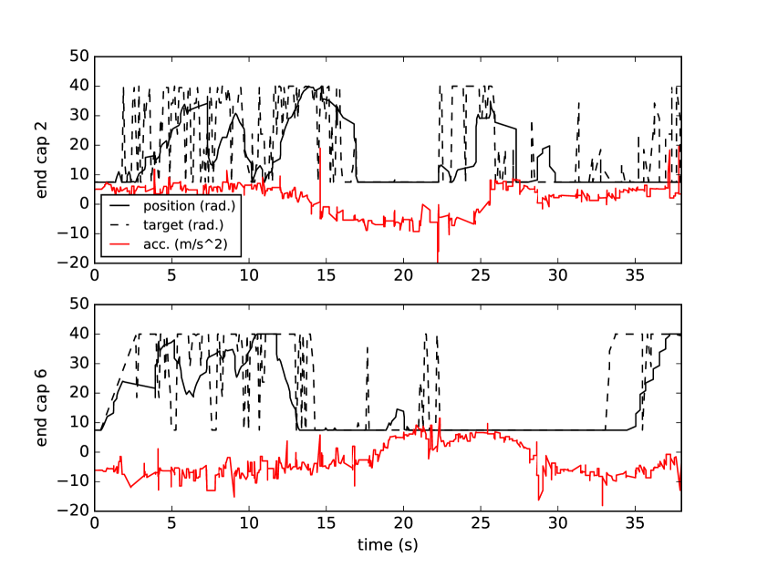
Figure 4: This plot shows actual motor positions (solid top), commanded target motor positions (black dotted), and single axis accelerometer data (solid bottom) for two disconnected end caps over the first $40\text{\,}\mathrm{s}$ of a trial. The learned policy commands target motor positions using accelerometer feedback. The actual motor positions lag behind due to motor dynamics and network UDP packet loss.

The open-loop policy was not able to produce any reasonable behavior on the real robot. The lack of performance exhibited by this policy is due to a mismatch between the dynamics of the simulated robot and the real robot. Specifically, the real SUPERball robot has friction in the cable routing system, which introduces noticeable hysteresis and non-linear behavior into the spring forces. Because of this, the real robot’s individual motor dynamics are not constant nor consistent for all cables and commanded positions. The policy uses these discrepancies to achieve faster locomotion in simulation, and the open-loop policy attempts to mimic this on the real robot, which does not work since the robot cannot reach the same motor positions over a fixed number of time steps as in simulation. The learned policy is able to adapt to the physical SUPERball robot by using feedback from the accelerometers, and it adopts a strategy that applies motor commands for a longer period of time in order to move the robot into the desired configuration, thus it is still able to produce a successful locomotion gait.

VII Discussion and Future Work

We presented a method for learning locomotion policies for tensegrity robots, by introducing several improvements to MDGPS that adapt the algorithm to tasks that require periodic behavior. We demonstrated learned policies for the SUPERball tensegrity robot in simulation that are efficient and perform well under a variety of environmental and robot parameters. We also demonstrated a learned policy that can be transferred directly to the real system to allow the physical SUPERball robot to roll. We showed that our learned locomotion policies are more effective and generalize better than open-loop policies and hand-engineered controllers.

One direction for future work is to extend our method to other locomotion systems, including other tensegrity robots and legged systems such as bipeds and quadrupeds. Since our method is specifically designed to tackle the growth in variance over long-horizon periodic motions, it would be well suited for learning periodic feedback policies for a wide range of locomotion platforms. Many of these platforms introduce new challenges such as instability, which should provide new insights and improvements for our method.

Finally, since learning the locomotion policies in this paper requires only a few hundred trials, a promising direction for future work is to perform the learning process itself directly on the physical hardware, which should require only a few hours of continuous operation. While we chose to use simulated training in this work, more complex hardware platforms or more elaborate environments may be difficult to simulate accurately. Furthermore, gradual changes to the hardware due to damage or wear-and-tear might require retraining of the policy in situ. Evaluating this application of our method would be an exciting direction for future work.

Acknowledgments

This work was supported in part by the DARPA SIMPLEX program and an NSF CAREER award. We appreciate the support, ideas, and feedback from members of the Berkeley Artificial Intelligence Research Lab and the Dynamic Tensegrity Robotics Lab. We are also grateful to Terry Fong and the NASA Ames Intelligent Robotics Group.

-A Additional Experimental Details

Because we train local policies with full state information $\mathbf{x}_{t}$ but learn a global policy that only receives an observation of the state $\mathbf{o}_{t}$ as input, we are able to train a global policy that operates under partial observability at test time while maintaining the simplicity of training the local policies on the full state. This separation between the local policies and global policy reflects prior work on tasks involving partial observability, where the intuition is that the local policies are trained in a controlled environment but the global policy must be able to adapt to a more general setting [36].

In our case, the full state $\mathbf{x}_{t}$ can only be obtained through either simulation or the use of an external state estimator system on the physical SUPERball robot [38]. In contrast, we choose an observation $\mathbf{o}_{t}$ that can be calculated directly from the sensors on the robot itself. This greatly simplifies the transfer from simulation to the real robot, as the learned policy is less prone to overfit to the simulation and takes actions directly based on the sensor measurements from the physical robot. Furthermore, because the goal of SUPERball and many other robots is deployment to unfamiliar, remote environments, the choice of an observation that relies only on the robot’s onboard sensors is very important, as it is unrealistic to expect the level of information and reliability that an external state estimator can provide. For a description of the state and observation, as well as the details and dimensionalities of the sensors, see Section VI-A.

Because the real-world sensors and actuators are noisy and imperfect, we attempt to model this in simulation by introducing noise on the input to the policy during training. We model measurement errors and sensor inaccuracies by adding Gaussian noise with mean 0 and variance equal to 10% of the range of the observation. To model sensor failure, latency, and network issues such as connection errors, we randomly drop observations 10% of the time. When the current observation is dropped, the previous observation is used as the input to the policy. We found that adding noise improves the generalization capabilities of the learned policy across conditions such as terrain, gravity, and motor failure, and we test against these conditions in Section VI-B.

-B Additional Experimental Results

	Two Local Policies,	One Local Policy
	Sequential	Full $10\text{\,}\mathrm{s}$
[HTML]D3D3D3 [HTML]D3D3D3Episodes Until	[HTML]D3D3D3	[HTML]D3D3D3
[HTML]D3D3D3 [HTML]D3D3D3Convergence	[HTML]D3D3D3$<700$	[HTML]D3D3D3$<800$
Average Distance
Traveled (m)	$3.156$	$1.228$

TABLE II: Comparison of sample efficiency and distance traveled at convergence of two local policies trained for $5\text{\,}\mathrm{s}$ each and one local policy trained for the full $10\text{\,}\mathrm{s}$. Note that our method of training sequential local policies requires fewer samples for convergence and demonstrates significantly better performance.

To show that our method of training sequential local policies is effective, we compared the results of training two sequential local policies for $5\text{\,}\mathrm{s}$ each against training one local policy for the full $10\text{\,}\mathrm{s}$, both using the trajectory-centric RL method detailed in [14]. We record the average distance traveled over five trials in Table II. The two local policies trained sequentially not only converges in fewer samples, but also settles into a much more effective rolling strategy that travels significantly farther over the course of $10\text{\,}\mathrm{s}$. These results show that, by training sequences of local policies over shorter horizons, we can achieve more efficient locomotion with fewer samples by decreasing the compounding effects of modeling errors and unstable policies over time.

References

- [1] J. Bruce, K. Caluwaerts, A. Iscen, A. P. Sabelhaus, and V. SunSpiral, “Design and evolution of a modular tensegrity robot platform,” in International Conference on Robotics and Automation (ICRA), 2014.
- [2] R. Tedrake, T. Zhang, and H. Seung, “Stochastic policy gradient reinforcement learning on a simple 3D biped,” in International Conference on Intelligent Robots and Systems (IROS), 2004.
- [3] N. Kohl and P. Stone, “Policy gradient reinforcement learning for fast quadrupedal locomotion,” in IROS, 2004.
- [4] R. Calendra, A. Seyfarth, J. Peters, and M. Deisenroth, “Bayesian optimization for learning gaits under uncertainty,” Annals of Mathematics and Artificial Intelligence (AMAI), vol. 76, pp. 5–23, 2016.
- [5] J. Kolter and A. Ng, “The Stanford LittleDog: A learning and rapid replanning approach to quadruped locomotion,” International Journal of Robotics Research (IJRR), vol. 30, no. 2, pp. 150–174, 2011.
- [6] M. Kalakrishnan, J. Buchli, P. Pastor, and S. Schaal, “Learning locomotion over rough terrain using terrain templates,” in IROS, 2009.
- [7] I. Mordatch, N. Mishra, C. Eppner, and P. Abbeel, “Combining model-based policy search with online model learning for control of physical humanoids,” in ICRA, 2016.
- [8] J. Schulman, S. Levine, P. Moritz, M. Jordan, and P. Abbeel, “Trust region policy optimization,” in International Conference on Machine Learning (ICML), 2015.
- [9] T. Lillicrap, J. Hunt, A. Pritzel, N. Heess, T. Erez, Y. Tassa, D. Silver, and D. Wierstra, “Continuous control with deep reinforcement learning,” in International Conference on Learning Representations (ICLR), 2016.
- [10] W. Montgomery and S. Levine, “Guided policy search as approximate mirror descent,” in Advances in Neural Information Processing Systems (NIPS), 2016.
- [11] T. Geng, B. Porr, and F. Wörgötter, “Fast biped walking with a reflexive controller and realtime policy searching,” in NIPS, 2006.
- [12] G. Endo, J. Morimoto, T. Matsubara, J. Nakanishi, and G. Cheng, “Learning CPG-based biped locomotion with a policy gradient method: Application to a humanoid robot,” IJRR, vol. 27, no. 2, 2008.
- [13] S. Levine and V. Koltun, “Guided policy search,” in ICML, 2013.
- [14] S. Levine and P. Abbeel, “Learning neural network policies with guided policy search under unknown dynamics,” in NIPS, 2014.
- [15] R. Motro, Tensegrity: Structural Systems of the Future. Kogan, 2003.
- [16] S. H. Juan and J. M. M. Tur, “Tensegrity frameworks: Static analysis review,” Mechanism and Machine Theory, vol. 43, no. 7, pp. 859 – 881, 2008.
- [17] M. Arsenault and C. M. Gosselin, “Kinematic and Static Analysis of a Three-degree-of-freedom Spatial Modular Tensegrity Mechanism,” IJRR, vol. 27, no. 8, pp. 951–966, 2008.
- [18] K. Kim, A. K. Agogino, A. Toghyan, D. Moon, L. Taneja, and A. M. Agogino, “Robust learning of tensegrity robot control for locomotion through form-finding,” in IROS, 2015.
- [19] A. Graells Rovira and J. M. Mirats-Tur, “Control and simulation of a tensegrity-based mobile robot,” Robotics and Autonomous Systems (RAS), vol. 57, no. 5, pp. 526–535, May 2009.
- [20] “NASA Tensegrity Robotics Toolkit,” ti.arc.nasa.gov/tech/asr/intelligent-robotics/tensegrity/ntrt.
- [21] A. Iscen, A. Agogino, V. SunSpiral, and K. Tumer, “Flop and roll: Learning robust goal-directed locomotion for a tensegrity robot,” in IROS, 2014.
- [22] B. Mirletz, P. Bhandal, R. D. Adams, A. K. Agogino, R. D. Quinn, and V. SunSpiral, “Goal directed CPG-based control for tensegrity spines with many degrees of freedom traversing irregular terrain,” Soft Robotics, vol. 2, pp. 165–176, 2015.
- [23] B. Mirletz, I. W. Park, R. D. Quinn, and V. SunSpiral, “Towards bridging the reality gap between tensegrity simulation and robotic hardware,” in IROS, 2015.
- [24] S. Collins, A. Ruina, R. Tedrake, and M. Wisse, “Efficient bipedal robots based on passive-dynamic walkers,” Science, vol. 307, pp. 1082–1085, 2005.
- [25] J. Pratt, C. Chew, A. Torres, P. Dilworth, and G. Pratt, “Virtual model control: An intuitive approach for bipedal locomotion,” IJRR, vol. 20, no. 2, pp. 129–143, 2001.
- [26] A. Seyfarth, H. Geyer, and H. Herr, “Swing-leg retraction: a simple control model for stable running,” Journal of Experimental Biology, vol. 206, pp. 2547–2555, 2003.
- [27] M. Deisenroth, G. Neumann, and J. Peters, “A survey on policy search for robotics,” Foundations and Trends in Robotics, vol. 2, no. 1-2, pp. 1–142, 2013.
- [28] M. Cutler, T. J. Walsh, and J. P. How, “Real-world reinforcement learning via multifidelity simulators,” IEEE Transactions on Robotics, vol. 31, pp. 655–671, 2016.
- [29] I. Mordatch, K. Lowrey, and E. Todorov, “Ensemble-CIO: Full-body dynamic motion planning that transfers to physical humanoids,” in IROS, 2015.
- [30] R. B. Fuller, Synergetics: Explorations in the Geometry of Thinking. Scribner, Jan. 1975.
- [31] K. Snelson, “Continuous tension, discontinuous compression structures. United States patent 3169611,” February 1965.
- [32] A. Sabelhaus, J. Bruce, K. Caluwaerts, P. Manovi, R. Firoozi, S. Dobi, A. M. Agogino, and V. SunSpiral, “System design and locomotion of SUPERball, an untethered tensegrity robot,” in ICRA, 2015.
- [33] J. Bagnell and J. Schneider, “Covariant policy search,” in International Joint Conference on Artificial Intelligence (IJCAI), 2003.
- [34] J. Peters and S. Schaal, “Reinforcement learning of motor skills with policy gradients,” Neural Networks, vol. 21, pp. 682––697, 2008.
- [35] J. Peters, K. Mülling, and Y. Altün, “Relative entropy policy search,” in AAAI Conference on Artificial Intelligence, 2010.
- [36] S. Levine, C. Finn, T. Darrell, and P. Abbeel, “End-to-end training of deep visuomotor policies,” Journal of Machine Learning Research (JMLR), vol. 17, pp. 1334–1373, 2016.
- [37] “FLANN: Fast Library for Approximate Nearest Neighbors,” http://www.cs.ubc.ca/research/flann/.
- [38] K. Caluwaerts, J. Bruce, J. M. Friesen, and V. SunSpiral, “State estimation for tensegrity robots,” in ICRA, 2016.