Fractional order statistic approximation for
nonparametric conditional quantile inference

Abstract

Using and extending fractional order statistic theory, we characterize the $O(n^{-1})$ coverage probability error of the previously proposed confidence intervals for population quantiles using $L$-statistics as endpoints in Hutson (1999). We derive an analytic expression for the $n^{-1}$ term, which may be used to calibrate the nominal coverage level to get $O\mathopen{}\mathclose{{}\left(n^{-3/2}[\log(n)]^{3}}\right)$ coverage error. Asymptotic power is shown to be optimal. Using kernel smoothing, we propose a related method for nonparametric inference on conditional quantiles. This new method compares favorably with asymptotic normality and bootstrap methods in theory and in simulations. Code is provided for both unconditional and conditional inference.

JEL classification: C21

Keywords: Dirichlet, high-order accuracy, inference-optimal bandwidth, kernel smoothing.

© 2016 by the authors. This manuscript version is made available under the CC-BY-NC-ND 4.0 license: http://creativecommons.org/licenses/by-nc-nd/4.0/

1 Introduction

Quantiles contain information about a distribution’s shape. Complementing the mean, they capture heterogeneity, inequality, and other measures of economic interest. Nonparametric conditional quantile models further allow arbitrary heterogeneity across regressor values. This paper concerns nonparametric inference on quantiles and conditional quantiles. In particular, we characterize the high-order accuracy of both Hutson’s (1999) $L$-statistic-based confidence intervals (CIs) and our new conditional quantile CIs.

Conditional quantiles appear across diverse topics because they are fundamental statistical objects. Such topics include wages (Hogg, 1975; Chamberlain, 1994; Buchinsky, 1994), infant birthweight (Abrevaya, 2001), demand for alcohol (Manning et al., 1995), and Engel curves (Alan et al., 2005; Deaton, 1997, pp. 81–82), which we examine in our empirical application.

We formally derive the coverage probability error (CPE) of the CIs from Hutson (1999), as well as asymptotic power of the corresponding hypothesis tests. Hutson (1999) had proposed CIs for quantiles using $L$-statistics (interpolating between order statistics) as endpoints and found they performed well, but formal proofs were lacking. Using the analytic $n^{-1}$ term we derive in the CPE, we provide a new calibration to achieve $O\bigl{(}n^{-3/2}[\log(n)]^{3}\bigr{)}$ CPE, analogous to the Ho and Lee (2005a) analytic calibration of the CIs in Beran and Hall (1993).

The theoretical results we develop contribute to the fractional order statistic literature and provide the basis for inference on other objects of interest explored in Goldman and Kaplan (2016b) and Kaplan (2014). In particular, Theorem 2 tightly links the distributions of $L$-statistics from the observed and ‘ideal’ (unobserved) fractional order statistic processes. Additionally, Lemma 7 provides Dirichlet PDF and PDF derivative approximations.

High-order accuracy is important for small samples (e.g., for experiments) as well as nonparametric analysis with small local sample sizes. For example, if $n=1024$ and there are five binary regressors, then the smallest local sample size cannot exceed $1024/2^{5}=32$.

For nonparametric conditional quantile inference, we apply the unconditional method to a local sample (similar to local constant kernel regression), smoothing over continuous covariates and also allowing discrete covariates. CPE is minimized by balancing the CPE of our unconditional method and the CPE from bias due to smoothing. We derive the optimal CPE and bandwidth rates, as well as a plug-in bandwidth when there is a single continuous covariate.

Our $L$-statistic method has theoretical and computational advantages over methods based on normality or an unsmoothed bootstrap. The theoretical bottleneck for our approach is the need to use a uniform kernel. Nonetheless, even if normality or bootstrap methods assume an infinitely differentiable conditional quantile function (and hypothetically fit an infinite-degree local polynomial), our CPE is still of smaller order with one or two continuous covariates. Our method also computes more quickly than existing methods (of reasonable accuracy), handling even more challenging tasks in 10–15 seconds instead of minutes.

Recent complementary work of Fan and Liu (2016) also concerns a “direct method” of nonparametric inference on conditional quantiles. They use a limiting Gaussian process to derive first-order accuracy in a general setting, whereas we use the finite-sample Dirichlet process to achieve high-order accuracy in an iid setting. Fan and Liu (2016) also provide uniform (over $X$) confidence bands. We suggest a confidence band from interpolating a growing number of joint CIs (as in Horowitz and Lee (2012)), although it will take additional work to rigorously justify. A different, ad hoc confidence band described in Section 6 generally outperformed others in our simulations.

If applied to a local constant estimator with a uniform kernel and the same bandwidth, the Fan and Liu (2016) approach is less accurate than ours due to the normal (instead of beta) reference distribution and integer (instead of interpolated) order statistics in their CI in equation (6). However, with other estimators like local polynomials or that in Donald et al. (2012), the Fan and Liu (2016) method is not necessarily less accurate. One limitation of our approach is that it cannot incorporate these other estimators, whereas Assumption GI(iii) in Fan and Liu (2016) includes any estimator that weakly converges (over a range of quantiles) to a Gaussian process with a particular structure. We compare further in our simulations. One open question is whether using our beta reference and interpolation can improve accuracy for the general Fan and Liu (2016) method beyond the local constant estimator with a uniform kernel; our Lemma 3 shows this at least retains first-order accuracy.

The order statistic approach to quantile inference uses the idea of the probability integral transform, which dates back to R. A. Fisher (1932), Karl Pearson (1933), and Neyman (1937). For continuous $X_{i}\stackrel{{\scriptstyle iid}}{{\sim}}F(\cdot)$, $F(X_{i})\stackrel{{\scriptstyle iid}}{{\sim}}\textrm{Unif}(0,1)$. Each order statistic from such an iid uniform sample has a known beta distribution for any sample size $n$. We show that the $L$-statistic linearly interpolating consecutive order statistics also follows an approximate beta distribution, with only $O(n^{-1})$ error in CDF. Although $O(n^{-1})$ is an asymptotic claim, the CPE of the CI using the $L$-statistic endpoint is bounded between the CPEs of the CIs using the two order statistics comprising the $L$-statistic, where one such CPE is too small and one is too big, for any sample size. This is an advantage over methods more sensitive to asymptotic approximation error.

Many other approaches to one-sample quantile inference have been explored. With Edgeworth expansions, Hall and Sheather (1988) and Kaplan (2015) obtain two-sided $O(n^{-2/3})$ CPE. With bootstrap, smoothing is necessary for high-order accuracy. This increases the computational burden and requires good bandwidth selection in practice. See Ho and Lee (2005b, §1) for a review of bootstrap methods. Smoothed empirical likelihood (Chen and Hall, 1993) also achieves nice theoretical properties, but with the same caveats.

Other order statistic-based CIs dating back to Thompson (1936) are surveyed in David and Nagaraja (2003, §7.1). Most closely related to Hutson (1999) is Beran and Hall (1993). Like Hutson (1999), Beran and Hall (1993) linearly interpolate order statistics for CI endpoints, but with an interpolation weight based on the binomial distribution. Although their proofs use expansions of the Rényi (1953) representation instead of fractional order statistic theory, their $n^{-1}$ CPE term is identical to that for Hutson (1999) other than the different weight. Prior work (e.g., Bickel, 1967; Shorack, 1972) has established asymptotic normality of $L$-statistics and convergence of the sample quantile process to a Gaussian limit process, but without such high-order accuracy.

The most apparent difference between the two-sided CIs of Beran and Hall (1993) and Hutson (1999) is that the former are symmetric in the order statistic index, whereas the latter are equal-tailed. This allows Hutson (1999) to be computed further into the tails. Additionally, our framework can be extended to CIs for interquantile ranges and two-sample quantile differences (Goldman and Kaplan, 2016b), which has not been done in the Rényi representation framework.

For nonparametric conditional quantile inference, in addition to the aforementioned Fan and Liu (2016) approach, Chaudhuri (1991) derives the pointwise asymptotic normal distribution of a local polynomial estimator. Qu and Yoon (2015) propose modified local linear estimators of the conditional quantile process that converge weakly to a Gaussian process, and they suggest using a type of bias correction that strictly enlarges a CI to deal with the first-order effect of asymptotic bias when using the MSE-optimal bandwidth rate.

Section 2 contains our theoretical results on fractional order statistic approximation, which are applied to unconditional quantile inference in Section 3. Section 4 concerns our new conditional quantile inference method. An empirical application and simulation results are in Sections 5 and 6, respectively. Proof sketches are collected in Appendix A, while the supplemental appendix contains full proofs. The supplemental appendix also contains details of the plug-in bandwidth calculations, as well as additional empirical and simulation results.

Notationally, $\phi(\cdot)$ and $\Phi(\cdot)$ are respectively the standard normal PDF and CDF, $\doteq$ should be read as “is equal to, up to smaller-order terms”, $\asymp$ as “has exact (asymptotic) rate/order of”, and $A_{n}=O(B_{n})$ as usual. Acronyms used are those for cumulative distribution function (CDF), confidence interval (CI), coverage probability (CP), coverage probability error (CPE), and probability density function (PDF).

2 Fractional order statistic theory

In this section, we introduce notation and present our core theoretical results linking unobserved ‘ideal’ fractional $L$-statistics with their observed counterparts.

Given an iid sample $\{X_{i}\}_{i=1}^{n}$ of draws from a continuous CDF denoted $F(\cdot)$, interest is in $Q(p)\equiv F^{-1}(p)$ for some $p\in(0,1)$, where $Q(\cdot)$ is the quantile function. For $u\in(0,1)$, the sample $L$-statistic commonly associated with $Q(u)$ is

$$\hat{Q}^{L}_{X}(u)\equiv(1-\epsilon)X_{n:k}+\epsilon X_{n:k+1},\quad k\equiv\lfloor u(n+1)\rfloor,\quad\epsilon\equiv u(n+1)-k,$$ (1)

where $\lfloor\cdot\rfloor$ is the floor function, $\epsilon$ is the interpolation weight, and $X_{n:k}$ denotes the $k$th order statistic (i.e., $k$th smallest sample value). While $Q(u)$ is latent and nonrandom, $\hat{Q}^{L}_{X}(u)$ is a random variable, and $\hat{Q}^{L}_{X}(\cdot)$ is a stochastic process, observed for arguments in $[1/(n+1),n/(n+1)]$.

Let $\Xi_{n}\equiv\mathopen{}\mathclose{{}\left\{k/(n+1)}\right\}_{k=1}^{n}$ denote the set of quantiles corresponding to the observed order statistics. If $u\in\Xi_{n}$, then no interpolation is necessary and $\hat{Q}^{L}_{X}(u)=X_{n:k}$. As detailed in Section 3, application of the probability integral transform yields exact coverage probability of a CI endpoint $X_{n:k}$ for $Q(p)$: $P\mathopen{}\mathclose{{}\left(X_{n:k}<F^{-1}(p)}\right)=P\mathopen{}\mathclose{{}\left(U_{n:k}<p}\right)$, where $U_{n:k}\equiv F(X_{n:k})\sim\beta(k,n+1-k)$ is equal in distribution to the $k$th order statistic from $U_{i}\stackrel{{\scriptstyle iid}}{{\sim}}\textrm{Unif}(0,1)$, $i=1,\ldots,n$ (Wilks, 1962, 8.7.4). However, we also care about $u\notin\Xi_{n}$, in which case $k$ is fractional. To better handle such fractional order statistics, we will present a tight link between the marginal distributions of the stochastic process $\hat{Q}^{L}_{X}(\cdot)$ and those of the analogous ‘ideal’ (I) process

$$\tilde{Q}^{I}_{X}(\cdot) \equiv F^{-1}\mathopen{}\mathclose{{}\left(\tilde{Q}^{I}_{U}(\cdot)}\right),$$ (2)

where $\tilde{Q}^{I}_{U}(\cdot)$ is the ideal (I) uniform (U) fractional order “statistic” process. We use a tilde in $\tilde{Q}^{I}_{X}(\cdot)$ and $\tilde{Q}^{I}_{U}(\cdot)$ instead of the hat like in $\hat{Q}^{L}_{X}(\cdot)$ to emphasize that the former are unobserved (hence not true statistics), whereas the latter is computable from the sample data.

This $\tilde{Q}^{I}_{U}(\cdot)$ in (2) is a Dirichlet process (Ferguson, 1973; Stigler, 1977) on the unit interval with index measure $\nu\mathopen{}\mathclose{{}\left([0,t]}\right)=(n+1)t$. Its univariate marginals are

$$\tilde{Q}^{I}_{U}(u)=U_{n:(n+1)u}\sim\beta\bigl{(}(n+1)u,(n+1)(1-u)\bigr{)}.$$ (3)

The marginal distribution of $\mathopen{}\mathclose{{}\left(\tilde{Q}^{I}_{U}(u_{1}),\tilde{Q}^{I}_{U}(u_{2})-\tilde{Q}^{I}_{U}(u_{1}),\ldots,\tilde{Q}^{I}_{U}(u_{k})-\tilde{Q}^{I}_{U}(u_{k-1})}\right)$ for $u_{1}<\cdots<u_{k}$ is Dirichlet with parameters $\mathopen{}\mathclose{{}\left(u_{1}(n+1),(u_{2}-u_{1})(n+1),\ldots,(u_{k}-u_{k-1})(n+1)}\right)$.

For all $u\in\Xi_{n}$, $\tilde{Q}^{I}_{X}(u)$ coincides with $\hat{Q}^{L}_{X}(u)$; they differ only in their interpolation between these points. Proposition 1 shows $\tilde{Q}^{I}_{X}(\cdot)$ and $\hat{Q}^{L}_{X}(\cdot)$ to be closely linked in probability.

Proposition 1.

For any fixed $\delta>0$ and $m>0$, define $\mathcal{U}^{\delta}\equiv\{u\in(0,1)\mid\forall\,t\in(u-m,u+m),f\mathopen{}\mathclose{{}\left(F^{-1}(t)}\right)\geq\delta\}$ and $\mathcal{U}^{\delta}_{n}\equiv\mathcal{U}^{\delta}\cap[\frac{1}{n+1},\frac{n}{n+1}]$; then, $\underset{u\in\mathcal{U}^{\delta}_{n}}{\sup}\mathopen{}\mathclose{{}\left|\tilde{Q}^{I}_{X}(u)-\hat{Q}^{L}_{X}(u)}\right|=O_{p}\mathopen{}\mathclose{{}\left(n^{-1}\log(n)}\right)$.

Although Proposition 1 motivates approximating the distribution of $\hat{Q}^{L}_{X}(u)$ by that of $\tilde{Q}^{I}_{X}(u)$, it is not relevant to high-order accuracy. In fact, its result is achieved by any interpolation between $X_{n:k}$ and $X_{n:k+1}$, not just $\hat{Q}^{L}_{X}(u)$; in contrast, the high-order accuracy we establish in Theorem 4 is only possible with precise interpolations like $\hat{Q}^{L}_{X}(u)$.

Next, we consider marginal distributions of fixed dimension $J$. We also consider the Gaussian approximation to the sampling distribution of fractional order statistics. It is well known that the centered and scaled empirical process for standard uniform random variables converges to a Brownian bridge. For standard Brownian bridge process $B(\cdot)$, we index by $u\in(0,1)$ the additional stochastic processes

$$\tilde{Q}^{B}_{U}(u)\equiv u+n^{-1/2}B(u)\qquad\textrm{and}\qquad\tilde{Q}^{B}_{X}(u)\equiv F^{-1}\bigl{(}\tilde{Q}^{B}_{U}(u)\bigr{)}.$$

The vector $\tilde{Q}^{I}_{U}(\mathbf{u})$ has an ordered Dirichlet distribution (i.e., the spacings between consecutive $\tilde{Q}^{I}_{U}(u_{j})$ follow a joint Dirichlet distribution), while $\tilde{Q}^{B}_{U}(\mathbf{u})$ is multivariate Gaussian. Lemma 7 in the appendix shows the close relationship between multivariate Dirichlet and Gaussian PDFs and PDF derivatives.

Theorem 2 shows the close distributional link among linear combinations of ideal, interpolated, and Gaussian-approximated fractional order statistics. Specifically, for arbitrary weight vector $\boldsymbol{\psi}\in\mathbb{R}^{J}$, we (distributionally) approximate

$$L^{L}\equiv\sum_{j=1}^{J}\psi_{j}\hat{Q}^{L}_{X}(u_{j})\quad \textrm{by}\quad L^{I}\equiv\sum_{j=1}^{J}\psi_{j}\tilde{Q}^{I}_{X}(u_{j}),$$ (4)

or alternatively $$\textrm{by}\quad L^{B}\equiv\sum_{j=1}^{J}\psi_{j}\tilde{Q}^{B}_{X}(u_{j}).$$

Our assumptions for this section are now presented, followed by the main theoretical result. Assumption A2 ensures that the first three derivatives of the quantile function are uniformly bounded in neighborhoods of the quantiles, $u_{j}$, which helps bound remainder terms in the proofs. We use bold for vectors and underline for matrices.

Assumption A1.

Sampling is iid: $X_{i}\stackrel{{\scriptstyle iid}}{{\sim}}F$, $i=1,\ldots,n$.

Assumption A2.

For each quantile $u_{j}$, the PDF $f(\cdot)$ (corresponding to CDF $F(\cdot)$ in A1) satisfies (i) $f(F^{-1}(u_{j}))>0$; (ii) $f^{\prime\prime}(\cdot)$ is continuous in some neighborhood of $F^{-1}(u_{j})$, i.e., $f\in C^{2}\mathopen{}\mathclose{{}\left(U_{\delta}\mathopen{}\mathclose{{}\left(F^{-1}(u_{j})}\right)}\right)$ with $U_{\delta}(x)$ denoting some $\delta$-neighborhood of point $x\in\mathbb{R}$.

Theorem 2.

Define $\underline{\mathcal{V}}$ as the $J\times J$ matrix with row $i$, column $j$ entries $\underline{\mathcal{V}}_{i,j}=\min\{u_{i},u_{j}\}-u_{i}u_{j}$. Let $\underline{\mathcal{A}}$ be the $J\times J$ matrix with main diagonal entries $\underline{\mathcal{A}}_{j,j}=f\mathopen{}\mathclose{{}\left(F^{-1}(u_{j})}\right)$ and zeros elsewhere, and let

$$\mathcal{V}_{\boldsymbol{\psi}}\equiv\boldsymbol{\psi}^{\prime}\mathopen{}\mathclose{{}\left(\underline{\mathcal{A}}^{-1}\underline{\mathcal{V}}\,\underline{\mathcal{A}}^{-1}}\right)\boldsymbol{\psi},\quad\mathbb{X}_{0}\equiv\sum_{j=1}^{J}\psi_{j}F^{-1}(u_{j}).$$

Let Assumption A1 hold, and let A2 hold at $\mathbf{\bar{u}}$. Given the definitions in (1), (2), and (4), the following results hold uniformly over $\mathbf{u}=\mathbf{\bar{u}}+o(1)$.

1. For a given constant $K$,

   $$P \bigg{(}L^{L}<\mathbb{X}_{0}+n^{-1/2}K\bigg{)}-P\bigg{(}L^{I}<\mathbb{X}_{0}+n^{-1/2}K\bigg{)}$$

   $$=\frac{K\exp\mathopen{}\mathclose{{}\left\{-K^{2}/(2\mathcal{V}_{\boldsymbol{\psi}})}\right\}}{\sqrt{2\pi\mathcal{V}_{\boldsymbol{\psi}}^{3}}}\mathopen{}\mathclose{{}\left[\sum_{j=1}^{J}\mathopen{}\mathclose{{}\left(\frac{\psi_{j}^{2}\epsilon_{j}(1-\epsilon_{j})}{f\mathopen{}\mathclose{{}\left[F^{-1}(u_{j})}\right]^{2}}}\right)}\right]n^{-1}+O\mathopen{}\mathclose{{}\left(n^{-3/2}[\log(n)]^{3}}\right),$$

   where the remainder is uniform over all $K$.

2. Uniformly over $K$,

   $$\sup_{K\in\mathbb{R}} \mathopen{}\mathclose{{}\left[P\bigg{(}L^{L}<\mathbb{X}_{0}+n^{-1/2}K\bigg{)}-P\bigg{(}L^{I}<\mathbb{X}_{0}+n^{-1/2}K\bigg{)}}\right]$$

   $$=\frac{e^{-1/2}}{\sqrt{2\pi\mathcal{V}_{\boldsymbol{\psi}}^{2}}}\mathopen{}\mathclose{{}\left[\sum_{j=1}^{J}\mathopen{}\mathclose{{}\left(\frac{\psi_{j}^{2}\epsilon_{j}(1-\epsilon_{j})}{f\mathopen{}\mathclose{{}\left[F^{-1}(u_{j})}\right]^{2}}}\right)}\right]n^{-1}+O\mathopen{}\mathclose{{}\left(n^{-3/2}[\log(n)]^{3}}\right),$$

   $$\sup_{K\in\mathbb{R}} \mathopen{}\mathclose{{}\left|P\bigg{(}L^{L}<\mathbb{X}_{0}+n^{-1/2}K\bigg{)}-P\bigg{(}L^{B}<\mathbb{X}_{0}+n^{-1/2}K\bigg{)}}\right|=O\mathopen{}\mathclose{{}\left(n^{-1/2}[\log(n)]^{3}}\right).$$

3 Quantile inference: unconditional

For inference on $Q(p)$, we continue to maintain A1 and A2. For $p\in(0,1)$ and confidence level $1-\alpha$, define $u^{h}(\alpha)$ and $u^{l}(\alpha)$ to solve

$$\alpha =P\Bigl{(}\tilde{Q}^{I}_{U}\mathopen{}\mathclose{{}\left(u^{h}(\alpha)}\right)<p\Bigr{)},\quad\alpha=P\Bigl{(}\tilde{Q}^{I}_{U}\mathopen{}\mathclose{{}\left(u^{l}(\alpha)}\right)>p\Bigr{)},$$ (5)

with $\tilde{Q}^{I}_{U}(u)\sim\beta\bigl{(}(n+1)u,(n+1)(1-u)\bigr{)}$ from (3), parallel to (7) and (8) in Hutson (1999).

One-sided CI endpoints for $Q(p)$ are $\hat{Q}^{L}_{X}(u^{h})$ or $\hat{Q}^{L}_{X}(u^{l})$. Two-sided CIs replace $\alpha$ with $\alpha/2$ in (5) and use both endpoints. This use of $\alpha/2$ yields the equal-tailed property; more generally, $t\alpha$ and $(1-t)\alpha$ can be used for $t\in(0,1)$.

Figure 1 visualizes an example. The beta distribution’s mean is $u^{h}$ (or $u^{l}$). Decreasing $u^{h}$ increases the probability mass in the shaded region below $u$, while increasing $u^{h}$ decreases the shaded region, and vice-versa for $u^{l}$. Solving (5) is a simple numerical search problem.

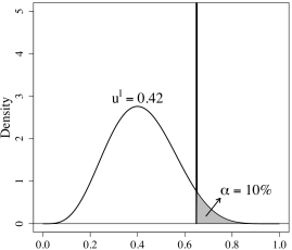
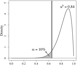
Figure 1: Example of one-sided CI endpoint determination, $n=11$, $p=0.65$, $\alpha=0.1$. Left: $u^{l}$ makes the shaded region’s area $P\bigl{(}\tilde{Q}^{I}_{U}(u^{l})>p\bigr{)}=\alpha$. Right: similarly, $u^{h}$ solves $P\bigl{(}\tilde{Q}^{I}_{U}(u^{h})<p\bigr{)}=\alpha$.

Lemma 3 shows the CI endpoint indices converge to $p$ at a $n^{-1/2}$ rate and may be approximated using quantiles of a normal distribution.

Lemma 3.

Let $z_{1-\alpha}$ denote the $(1-\alpha)$-quantile of a standard normal distribution, $z_{1-\alpha}\equiv\Phi^{-1}(1-\alpha)$. From the definitions in (5), the values $u^{l}(\alpha)$ and $u^{h}(\alpha)$ can be approximated as

$$u^{l}(\alpha) =p-n^{-1/2}z_{1-\alpha}\sqrt{p(1-p)}-\frac{2p-1}{6n}(z_{1-\alpha}^{2}+2)+O(n^{-3/2}),$$

$$u^{h}(\alpha) =p+n^{-1/2}z_{1-\alpha}\sqrt{p(1-p)}-\frac{2p-1}{6n}(z_{1-\alpha}^{2}+2)+O(n^{-3/2}).$$

For the lower one-sided CI, using (5), the $1-\alpha$ CI from Hutson (1999) is

$$\Bigl{(}-\infty,\hat{Q}^{L}_{X}\bigl{(}u^{h}(\alpha)\bigr{)}\Bigr{)}.$$ (6)

Coverage probability is

$$P \mathopen{}\mathclose{{}\left\{Q(p)\in\mathopen{}\mathclose{{}\left(-\infty,\hat{Q}^{L}_{X}\bigl{(}u^{h}(\alpha)\bigr{)}}\right)}\right\}=P\mathopen{}\mathclose{{}\left(\hat{Q}^{L}_{X}\bigl{(}u^{h}(\alpha)\bigr{)}>Q(p)}\right)$$

$$\!\!\!\!\stackrel{{\scriptstyle\textrm{Thm \ref{thm:cdferror}}}}{{=}}P\mathopen{}\mathclose{{}\left(\tilde{Q}^{I}_{X}\bigl{(}u^{h}(\alpha)\bigr{)}>Q(p)}\right)+\frac{\epsilon_{h}(1-\epsilon_{h})z_{1-\alpha}\exp\{-z_{1-\alpha}^{2}/2\}}{\sqrt{2\pi}u^{h}(\alpha)(1-u^{h}(\alpha))}n^{-1}+O\mathopen{}\mathclose{{}\left(n^{-3/2}[\log(n)]^{3}}\right)$$

$$=1-\alpha+\frac{\epsilon_{h}(1-\epsilon_{h})z_{1-\alpha}\phi(z_{1-\alpha})}{p(1-p)}n^{-1}+O\mathopen{}\mathclose{{}\left(n^{-3/2}[\log(n)]^{3}}\right),$$

where $\phi(\cdot)$ is the standard normal PDF and the $n^{-1}$ term is non-negative. Similar to the Ho and Lee (2005a) calibration, we can remove the analytic $n^{-1}$ term with the calibrated CI

$$\mathopen{}\mathclose{{}\left(-\infty,\hat{Q}^{L}_{X}\mathopen{}\mathclose{{}\left(u^{h}\mathopen{}\mathclose{{}\left(\alpha+\frac{\epsilon_{h}(1-\epsilon_{h})z_{1-\alpha}\phi(z_{1-\alpha})}{p(1-p)}n^{-1}}\right)}\right)}\right),$$ (7)

which has CPE of order $O\mathopen{}\mathclose{{}\left(n^{-3/2}[\log(n)]^{3}}\right)$. We follow convention and define $\textrm{CPE}\equiv\textrm{CP}-(1-\alpha)$, where CP is the actual coverage probability and $1-\alpha$ the desired confidence level.

By parallel argument, Hutson’s (1999) uncalibrated upper one-sided and two-sided CIs also have $O(n^{-1})$ CPE, or $O\mathopen{}\mathclose{{}\left(n^{-3/2}[\log(n)]^{3}}\right)$ with calibration. For the upper one-sided case, again using (5), the $1-\alpha$ Hutson CI and our calibrated CI are respectively given by

$$\mathopen{}\mathclose{{}\left(\hat{Q}^{L}_{X}\bigl{(}u^{l}(\alpha)\bigr{)},\infty}\right),\quad\mathopen{}\mathclose{{}\left(\hat{Q}^{L}_{X}\mathopen{}\mathclose{{}\left(u^{l}\mathopen{}\mathclose{{}\left(\alpha+\frac{\epsilon_{\ell}(1-\epsilon_{\ell})z_{1-\alpha}\phi(z_{1-\alpha})}{p(1-p)}n^{-1}}\right)}\right),\infty}\right),$$ (8)

and for equal-tailed two-sided CIs,

$$\mathopen{}\mathclose{{}\left(\hat{Q}^{L}_{X}\mathopen{}\mathclose{{}\left[u^{l}\mathopen{}\mathclose{{}\left(\alpha/2}\right)}\right],\hat{Q}^{L}_{X}\mathopen{}\mathclose{{}\left(u^{h}\mathopen{}\mathclose{{}\left(\alpha/2}\right)}\right)}\right)\quad\textrm{and}$$ (9)

$$\begin{split}&\Bigg{(}\enspace\hat{Q}^{L}_{X}\mathopen{}\mathclose{{}\left(u^{l}\mathopen{}\mathclose{{}\left(\frac{\alpha}{2}+\frac{\epsilon_{\ell}(1-\epsilon_{\ell})z_{1-\alpha/2}\phi(z_{1-\alpha/2})}{p(1-p)}n^{-1}}\right)}\right),\\ &\qquad\quad\hat{Q}^{L}_{X}\mathopen{}\mathclose{{}\left(u^{h}\mathopen{}\mathclose{{}\left(\frac{\alpha}{2}+\frac{\epsilon_{h}(1-\epsilon_{h})z_{1-\alpha/2}\phi(z_{1-\alpha/2})}{p(1-p)}n^{-1}}\right)}\right)\enspace\Bigg{)}.\end{split}$$ (10)

Without calibration, in all cases the $n^{-1}$ CPE term is non-negative (indicating over-coverage).

For relatively extreme quantiles $p$ (given $n$), the $L$-statistic method cannot be computed because the $(n+1)$th (or zeroth) order statistic is needed. In such cases, our code uses the Edgeworth expansion-based CI in Kaplan (2015). Alternatively, if bounds on $X$ are known a priori, they may be used in place of these “missing” order statistics to generate conservative CIs. Regardless, as $n\to\infty$, the range of computable quantiles approaches $(0,1)$.

The hypothesis tests corresponding to all the foregoing CIs achieve optimal asymptotic power against local alternatives. The sample quantile is a semiparametric efficient estimator, so it suffices to show that power is asymptotically first-order equivalent to that of the test based on asymptotic normality. Theorem 4 collects all of our results on coverage and power.

Theorem 4.

Let $z_{\alpha}$ denote the $\alpha$-quantile of the standard normal distribution, and let $\epsilon_{h}=(n+1)u^{h}(\alpha)-\lfloor(n+1)u^{h}(\alpha)\rfloor$ and $\epsilon_{\ell}=(n+1)u^{l}(\alpha)-\lfloor(n+1)u^{l}(\alpha)\rfloor$. Let Assumption A1 hold, and let A2 hold at $p$. Then, we have the following.

1. The one-sided lower and upper CIs in (6) and (8) have coverage probability

   $$1-\alpha+\frac{\epsilon(1-\epsilon)z_{1-\alpha}\phi(z_{1-\alpha})}{p(1-p)}n^{-1}+O\mathopen{}\mathclose{{}\left(n^{-3/2}[\log(n)]^{3}}\right),$$

   with $\epsilon=\epsilon_{h}$ for the former and $\epsilon=\epsilon_{\ell}$ for the latter.

2. The equal-tailed, two-sided CI in (9) has coverage probability

   $$1-\alpha+\frac{[\epsilon_{h}(1-\epsilon_{h})+\epsilon_{\ell}(1-\epsilon_{\ell})]z_{1-\alpha/2}\phi(z_{1-\alpha/2})}{p(1-p)}n^{-1}+O\mathopen{}\mathclose{{}\left(n^{-3/2}[\log(n)]^{3}}\right).$$

3. The calibrated one-sided lower, one-sided upper, and two-sided equal-tailed CIs given in (7), (8), and (10), respectively, have $O\mathopen{}\mathclose{{}\left(n^{-3/2}[\log(n)]^{3}}\right)$ CPE.

4. The asymptotic probabilities of excluding $D_{n}=Q(p)+\kappa n^{-1/2}$ from lower one-sided (l), upper one-sided (u), and equal-tailed two-sided (t) CIs (i.e., asymptotic power of the corresponding hypothesis tests) are

   $$\mathcal{P}_{n}^{l}(D_{n}) \to\Phi\mathopen{}\mathclose{{}\left(z_{\alpha}+S}\right),\;\mathcal{P}_{n}^{u}(D_{n})\to\Phi\mathopen{}\mathclose{{}\left(z_{\alpha}-S}\right),\;\mathcal{P}_{n}^{t}(D_{n})\to\Phi\mathopen{}\mathclose{{}\left(z_{\alpha/2}+S}\right)+\Phi\mathopen{}\mathclose{{}\left(z_{\alpha/2}-S}\right),$$

   where $S\equiv\kappa f(F^{-1}(p))/\sqrt{p(1-p)}$.

The equal-tailed property of our two-sided CIs is a type of median-unbiasedness. If $(\hat{L},\hat{H})$ is a CI for scalar $\theta$, then an equal-tailed CI is “unbiased” under loss function $L(\theta,\hat{L},\hat{H})=\max\{0,\theta-\hat{H},\hat{L}-\theta\}$, as defined in (5) of Lehmann (1951). This median-unbiased property may be desirable (e.g., Andrews and Guggenberger, 2014, footnote 11), although it is different than the usual “unbiasedness” where a CI is the inversion of an unbiased test. More generally, in (9), we could replace $u^{l}(\alpha/2)$ and $u^{h}(\alpha/2)$ by $u^{l}(t\alpha)$ and $u^{h}((1-t)\alpha)$ for $t\in[0,1]$. Different $t$ may achieve different optimal properties, which we leave to future work.

4 Quantile inference: conditional

4.1 Setup and bias

Let $Q_{Y|X}(u;x)$ be the conditional $u$-quantile function of scalar outcome $Y$ given conditioning vector $X\in\mathcal{X}\subset\mathbb{R}^{d}$, evaluated at $X=x$. The object of interest is $Q_{Y|X}(p;x_{0})$, for $p\in(0,1)$ and interior point $x_{0}$. The sample $\{Y_{i},X_{i}\}_{i=1}^{n}$ is drawn iid. Without loss of generality, let $x_{0}=0$.

If $X$ is discrete so that $P(X=0)>0$, we can take the subsample with $X_{i}=0$ and compute a CI from the corresponding $Y_{i}$ values, using the method in Section 3. Even with dependence like strong mixing among the $X_{i}$, CPE is the same $O(n^{-1})$ from Theorem 4 as long as the subsample’s $Y_{i}$ are independent draws from the same $Q_{Y|X}(\cdot;0)$ and $N_{n}\stackrel{{\scriptstyle a.s.}}{{\asymp}}n$.

If $X$ is continuous, then $P(X_{i}=0)=0$, so observations with $X_{i}\neq 0$ must be included. If $X$ contains mixed continuous and discrete components, then we can apply our method for continuous $X$ to each subsample corresponding to each unique value of the discrete subvector of $X$. The asymptotic rates are unaffected by the presence of discrete variables (although the finite-sample consequences may deserve more attention), so we focus on the case where all components of $X$ are continuous.

We now present definitions and assumptions, continuing the normalization $x_{0}=0$.

Definition 1 (local smoothness).

Following Chaudhuri (1991, pp. 762–3): if, in a neighborhood of the origin, function $g(\cdot)$ is continuously differentiable through order $k$, and its $k$th derivatives are uniformly Hölder continuous with exponent $\gamma\in(0,1]$, then $g(\cdot)$ has “local smoothness” of degree $s=k+\gamma$.

Assumption A3.

Sampling of $(Y_{i},X_{i}^{\prime})^{\prime}$ is iid, for continuous scalar $Y_{i}$ and continuous vector $X_{i}\in\mathcal{X}\subseteq\mathbb{R}^{d}$. The point of interest $X=0$ is in the interior of $\mathcal{X}$, and the quantile of interest is $p\in(0,1)$.

Assumption A4.

The marginal density of $X$, denoted $f_{X}(\cdot)$, satisfies $0<f_{X}(0)<\infty$ and has local smoothness $s_{X}=k_{X}+\gamma_{X}>0$.

Assumption A5.

For all $u$ in a neighborhood of $p$, $Q_{Y|X}(u;\cdot)$ (as a function of the second argument) has local smoothness $s_{Q}=k_{Q}+\gamma_{Q}>0$.

Assumption A6.

As $n\to\infty$, the bandwidth satisfies (i) $h\to 0$, (i’) $h^{b+d/2}\sqrt{n}\to 0$ with $b\equiv\min\{s_{Q},s_{X}+1,2\}$, (ii) $nh^{d}/[\log(n)]^{2}\to\infty$.

Assumption A7.

For all $u$ in a neighborhood of $p$ and all $x$ in a neighborhood of the origin, $f_{Y|X}\mathopen{}\mathclose{{}\left(Q_{Y|X}(u;x);x}\right)$ is uniformly bounded away from zero.

Assumption A8.

For all $y$ in a neighborhood of $Q_{Y|X}(p;0)$ and all $x$ in a neighborhood of the origin, $f_{Y|X}\mathopen{}\mathclose{{}\left(y;x}\right)$ has a second derivative in its first argument ($y$) that is uniformly bounded and continuous in $y$, having local smoothness $s_{Y}=k_{Y}+\gamma_{Y}>2$.

Definition 2 refers to a window whose size depends on $h$: $C_{h}=[-h,h]$ if $d=1$, or more generally a hypercube as in Chaudhuri (1991, pp. 763): letting $\|\cdot\|_{\infty}$ denote the $L_{\infty}$-norm,

$$C_{h} \equiv\{x:x\in\mathbb{R}^{d},\|x\|_{\infty}\leq h\},\quad N_{n}\equiv\#\bigl{(}\{Y_{i}:X_{i}\in C_{h},1\leq i\leq n\}\bigr{)}.$$ (11)

Definition 2 (local sample).

Using $C_{h}$ and $N_{n}$ defined in (11), the “local sample” consists of $Y_{i}$ values from observations with $X_{i}\in C_{h}\subset\mathbb{R}^{d}$, and the “local sample size” is $N_{n}$. Additionally, let the local quantile function $Q_{Y|X}(p;C_{h})$ be the $p$-quantile of $Y$ given $X\in C_{h}$, satisfying $p=P\mathopen{}\mathclose{{}\left(Y<Q_{Y|X}(p;C_{h})\mid X\in C_{h}}\right)$; similarly define the local CDF $F_{Y|X}(\cdot;C_{h})$, local PDF $f_{Y|X}(\cdot;C_{h})$, and derivatives thereof.

Given fixed values of $n$ and $h$, Assumption A3 implies that the $Y_{i}$ in the local sample are independent and identically distributed, which is needed to apply Theorem 4. However, they do not have the quantile function of interest, $Q_{Y|X}(\cdot;0)$, but rather the biased $Q_{Y|X}(\cdot;C_{h})$. This is like drawing a global (any $X_{i}$) iid sample of wages, $Y_{i}$, and restricting it to observations in Japan ($X\in C_{h}$) when our interest is only in Tokyo ($X=0$): our restricted $Y_{i}$ constitute an iid sample from Japan, but the $p$-quantile wage in Japan may differ from that in Tokyo. Assumptions A4–A6(i) and A8 are necessary for the calculation of this bias, $Q_{Y|X}(p;C_{h})-Q_{Y|X}(p;0)$, in Lemma 5. Assumptions A6(ii) and A7 (and A3) ensure $N_{n}\stackrel{{\scriptstyle a.s.}}{{\to}}\infty$. Assumptions A7 and A8 are conditional versions of Assumptions A2(i) and A2(ii), respectively. Their uniformity ensures uniformity of the remainder term in Theorem 4, accounting for the fact that the local sample’s distribution, $F_{Y|X}(\cdot;C_{h})$, changes with $n$ (through $h$ and $C_{h}$).

From A6(i), asymptotically $C_{h}$ is entirely contained within the neighborhoods implicit in A4, A5, and A8. This in turn allows us to examine only a local neighborhood around $p$ (e.g., as in A5) since the CI endpoints converge to the true value at a $N_{n}^{-1/2}$ rate.

The $X_{i}$ being iid helps guarantee that $N_{n}$ is almost surely of order $nh^{d}$. The $h^{d}$ comes from the volume of $C_{h}$. Larger $h$ lowers CPE via $N_{n}$ but raises CPE via bias. This tradeoff determines the optimal rate at which $h\to 0$ as $n\to\infty$. Using Theorem 4 and additional results on CPE from bias below, we determine the optimal value of $h$.

Definition 3 (steps to compute CI for $Q_{Y|X}(p;0)$).

First, $C_{h}$ and $N_{n}$ are calculated as in Definition 2. Second, using the $Y_{i}$ from observations with $X_{i}\in C_{h}$, a $p$-quantile CI is constructed as in Hutson (1999). If additional discrete conditioning variables exist, then repeat separately for each combination of discrete conditioning values. This procedure may be repeated for any number of $x_{0}$. For the bandwidth, we recommend the formulas in Section 4.3.

The bias characterized in Lemma 5 is the difference between these two population conditional quantiles.

Lemma 5.

Define $b$ as in A6 and let $B_{h}\equiv Q_{Y|X}(p;C_{h})-Q_{Y|X}(p;0)$. If Assumptions A4, A5, A6(i), A7, and A8 hold, then the bias is of order $|B_{h}|=O(h^{b})$. Defining

$$\xi_{p}\equiv Q_{Y|X}(p;0),\quad F_{Y|X}^{(0,1)}(\xi_{p};0)\equiv\mathopen{}\mathclose{{}\left.\frac{\partial}{\partial x}F_{Y|X}(\xi_{p};x)}\right|_{x=0},\quad F_{Y|X}^{(0,2)}(\xi_{p};0)\equiv\mathopen{}\mathclose{{}\left.\frac{\partial^{2}}{\partial x^{2}}F_{Y|X}(\xi_{p};x)}\right|_{x=0},$$

with $d=1$, $k_{X}\geq 1$, and $k_{Q}\geq 2$, the bias is

$$B_{h}=-h^{2}\frac{f_{X}(0)F_{Y|X}^{(0,2)}(\xi_{p};0)+2f_{X}^{\prime}(0)F_{Y|X}^{(0,1)}(\xi_{p};0)}{6f_{X}(0)f_{Y|X}(\xi_{p};0)}+o(h^{2}).$$ (12)

Equation (12) is the same as in Bhattacharya and Gangopadhyay (1990), who derive it using different arguments.

4.2 Optimal CPE order

The CPE-optimal bandwidth minimizes the sum of the two dominant high-order CPE terms. It must be small enough to control the $O(h^{b}+N_{n}h^{2b})$ (two-sided) CPE from bias, but large enough to control the $O(N_{n}^{-1})$ CPE from applying the unconditional $L$-statistic method. The following theorem summarizes optimal bandwidth and CPE results.

Theorem 6.

Let Assumptions A3–A8 hold. The following results are for the method in Definition 3. For a one-sided CI, the bandwidth $h^{*}$ minimizing CPE has rate $h^{*}\asymp n^{-3/(2b+3d)}$, corresponding to CPE of order $O(n^{-2b/(2b+3d)})$. For a two-sided CI, the optimal bandwidth rate is $h^{*}\asymp n^{-1/(b+d)}$, and the optimal CPE is $O(n^{-b/(b+d)})$. Using the calibration in Section 3, if $p=1/2$, then the nearly (up to $\log(n)$) CPE-optimal two-sided bandwidth rate is $h^{*}\asymp n^{-5/(4b+5d)}$, yielding CPE of order $O\mathopen{}\mathclose{{}\left(n^{-6b/(4b+5d)}[\log(n)]^{3}}\right)$; if $p\neq 1/2$, then $h^{*}\asymp n^{-3/(b+3d)}$ and CPE is $O\mathopen{}\mathclose{{}\left(n^{-3b/(2b+6d)}[\log(n)]^{3}}\right)$. The nearly CPE-optimal calibrated one-sided bandwidth rate is $h^{*}\asymp n^{-2/(b+2d)}$, yielding CPE of order $O\mathopen{}\mathclose{{}\left(n^{-3b/(2b+4d)}[\log(n)]^{3}}\right)$.

As detailed in the supplemental appendix, Theorem 6 implies that for the most common values of dimension $d$ and most plausible values of smoothness $s_{Q}$, even our uncalibrated method is more accurate than inference based on asymptotic normality with a local polynomial estimator. The same comparisons apply to basic bootstraps, which claim no refinement over asymptotic normality; in this (quantile) case, even Studentization does not improve theoretical CPE without the added complications of smoothed or $m$-out-of-$n$ bootstraps.

The only opportunity for normality to yield smaller CPE is to greatly reduce bias by using a very large local polynomial if $s_{Q}$ is large; our approach implicitly uses a uniform kernel, so bias reduction beyond $O(h^{2})$ is impossible. Nonetheless, our method has smaller CPE when $d=1$ or $d=2$ even if $s_{Q}=\infty$, and in other cases the necessary local polynomial degree may be prohibitively large given common sample sizes.

Figure 2: Two-sided CPE comparison between new (“L-stat”) method and the local polynomial asymptotic normality method based on Chaudhuri (1991). Left: with $s_{Q}=2$ and $s_{X}=1$, writing CPE as $n^{\kappa}$, comparison of $\kappa$ for different methods and different values of $d$. Right: required smoothness $s_{Q}$ for the local polynomial normality-based CPE to match that of L-stat, as well as the corresponding number of terms in the local polynomial, for different $d$.

Figure 2 (left panel) shows that if $s_{Q}=2$ and $s_{X}=1$, then the optimal CPE from asymptotic normality is always larger (worse) than our method’s CPE. As shown in the supplement, CPE with normality is nearly $O\bigl{(}n^{-2/(4+2d)}\bigr{)}$. With $d=1$, this is $O\bigl{(}n^{-1/3}\bigr{)}$, much larger than our two-sided $O\bigl{(}n^{-2/3}\bigr{)}$. With $d=2$, $O\bigl{(}n^{-1/4}\bigr{)}$ is larger than our $O\bigl{(}n^{-1/2}\bigr{)}$. It remains larger for all $d$ since the bias is the same for both methods while the unconditional $L$-statistic inference is more accurate than normality.

Figure 2 (right panel) shows the required amount of smoothness and local polynomial degree for asymptotic normality to match our method’s CPE. For the most common cases of $d=1$ and $d=2$, two-sided CPE with normality is larger even with infinite smoothness and a hypothetical infinite-degree polynomial. With $d=3$, to match our CPE, normality needs $s_{Q}\geq 12$ and a local polynomial of degree $k_{Q}\geq 11$. Since interaction terms are required, an $11$th-degree polynomial has $\sum_{T=d-1}^{k_{Q}+d-1}\binom{T}{d-1}=364$ terms, which requires a large $N_{n}$ (and yet larger $n$). As $d\to\infty$, the required number of terms in the local polynomial only grows larger and may be prohibitive in realistic finite samples.

4.3 Plug-in bandwidth

We propose a feasible bandwidth value with the CPE-optimal rate. To avoid recursive dependence on $\epsilon$ (the interpolation weight), we fix its value. This does not achieve the theoretical optimum, but it remains close even in small samples and seems to work well in practice. The CPE-optimal bandwidth value derivation is shown for $d=1$ in the supplemental appendix; a plug-in version is implemented in our code. For reference, the plug-in bandwidth expressions are collected here. The $\alpha$-quantile of $N(0,1)$ is again denoted $z_{\alpha}$. We let $\hat{B}_{h}$ denote the estimator of bias term $B_{h}$; $\hat{f}_{X}$ the estimator of $f_{X}(x_{0})$; $\hat{f}_{X}^{\prime}$ the estimator of $f_{X}^{\prime}(x_{0})$; $\hat{F}_{Y|X}^{(0,1)}$ the estimator of $F_{Y|X}^{(0,1)}(\xi_{p};x_{0})$; and $\hat{F}_{Y|X}^{(0,2)}$ the estimator of $F_{Y|X}^{(0,2)}(\xi_{p};x_{0})$, with notation from Lemma 5.

When $d=1$, the following are our CPE-optimal plug-in bandwidths.

• For one-sided inference, let

  $$\hat{h}_{+-} =n^{-3/7}\mathopen{}\mathclose{{}\left(\frac{z_{1-\alpha}}{3\mathopen{}\mathclose{{}\left[p(1-p)\hat{f}_{X}}\right]^{1/2}\mathopen{}\mathclose{{}\left[\hat{f}_{X}\hat{F}_{Y|X}^{(0,2)}+2\hat{f}_{X}^{\prime}\hat{F}_{Y|X}^{(0,1)}}\right]}}\right)^{2/7},$$ (13)

  $$\hat{h}_{++} =-0.770\hat{h}_{+-}.$$ (14)

  For lower one-sided inference, $\hat{h}_{+-}$ should be used if $\hat{B}_{h}<0$, and $\hat{h}_{++}$ otherwise. For upper one-sided inference, $\hat{h}_{++}$ should be used if $\hat{B}_{h}<0$, and $\hat{h}_{+-}$ otherwise.

• For two-sided inference with general $p\in(0,1)$,

  $$\hat{h} =n^{-1/3}\mathopen{}\mathclose{{}\left(\frac{(\hat{B}_{h}/|\hat{B}_{h}|)(1-2p)+\sqrt{(1-2p)^{2}+4}}{2\mathopen{}\mathclose{{}\left|\hat{f}_{X}\hat{F}_{Y|X}^{(0,2)}+2\hat{f}_{X}^{\prime}\hat{F}_{Y|X}^{(0,1)}}\right|}}\right)^{1/3},$$ (15)

  which simplifies to $\hat{h}=n^{-1/3}\bigl{|}\hat{f}_{X}\hat{F}_{Y|X}^{(0,2)}+2\hat{f}_{X}^{\prime}\hat{F}_{Y|X}^{(0,1)}\bigr{|}^{-1/3}$ with $p=0.5$.

While we suggest the CPE-optimal bandwidths for moderate $n$, we suggest shifting toward a larger bandwidth as $n\to\infty$. Once CPE is small over a range of bandwidths, a larger bandwidth in that range is preferable since it yields shorter CIs. As an initial suggestion, we use a coefficient of $\max\{1,n/1000\}^{5/60}$ that keeps the CPE-optimal bandwidth for $n\leq 1000$ and then moves toward a $n^{-1/20}$ under-smoothing of the MSE-optimal bandwidth rate, as in Fan and Liu (2016, p. 205).

5 Empirical application

We present an application of our $L$-statistic inference to Engel (1857) curves. Code is available from the latter author’s website, and the data are publicly available.

Banks et al. (1997) argue that a linear Engel curve is sufficient for certain categories of expenditure, while adding a quadratic term suffices for others. Their Figure 1 shows nonparametrically estimated mean Engel curves (budget share $W$ against log total expenditure $\ln(X)$) with $95\%$ pointwise CIs at the deciles of the total expenditure distribution, using a subsample of 1980–1982 U.K. Family Expenditure Survey (FES) data.

We present a similar examination, but for quantile Engel curves in the 2001–2012 U.K. Living Costs and Food Surveys (Office for National Statistics and Department for Environment, Food and Rural Affairs, 2012), which is a successor to the FES. We examine the same four categories as in the original analysis: food; fuel, light, and power (“fuel”); clothing and footwear (“clothing”); and alcohol. We use the subsample of households with one adult male and one adult female (and possibly children) living in London or the South East, leaving $8{,}528$ observations. Expenditure amounts are adjusted to 2012 nominal values using annual CPI data.

Table 1: $L$-statistic $99\%$ CIs for various unconditional quantiles ($p$) of the budget share distribution, for different categories of expenditure described in the text.

Category	$p=0.5$	$p=0.75$	$p=0.9$
food	(0.1532,0.1580)	(0.2095,0.2170)	(0.2724,0.2818)
fuel	(0.0275,0.0289)	(0.0447,0.0470)	(0.0692,0.0741)
clothing	(0.0135,0.0152)	(0.0362,0.0397)	(0.0697,0.0761)
alcohol	(0.0194,0.0226)	(0.0548,0.0603)	(0.1012,0.1111)

Table 1 shows unconditional $L$-statistic CIs for various quantiles of the budget share distributions for the four expenditure categories. (Due to the large sample size, calibrated CIs are identical at the precision shown.) These capture some population features, but the conditional quantiles are of more interest.

Figure 3: Joint (over the nine expenditure levels) $90\%$ confidence intervals for quantile Engel curves: food (top left), fuel (top right), clothing (bottom left), and alcohol (bottom right).

Figure 3 is comparable to Figure 1 of Banks et al. (1997) but with $90\%$ joint (over the nine expenditure levels) CIs instead of $95\%$ pointwise CIs, alongside quadratic quantile regression estimates. (To get joint CIs, we simply use the Bonferroni adjustment and compute $1-\alpha/9$ pointwise CIs.) Joint CIs are more intuitive for assessing the shape of a function since they jointly cover all corresponding points on the true curve with $90\%$ probability, rather than any given single point. The CIs are interpolated only for visual convenience. Although some of the joint CI shapes do not look quadratic at first glance, the only cases where the quadratic fit lies outside one of the intervals are for alcohol at the conditional median and clothing at the conditional upper quartile, and neither is a radical departure. With a $90\%$ confidence level and 12 confidence sets, we would not be surprised if one or two did not cover the true quantile Engel curve completely. Importantly, the CIs are relatively precise, too; the linear fit is rejected in 8 of 12 cases. Altogether, this evidence suggests that the benefits of a quadratic (but not linear) approximation may outweigh the cost of approximation error.

The supplemental appendix includes a similar figure but with a nonparametric (instead of quadratic) conditional quantile estimate along with joint CIs from Fan and Liu (2016).

6 Simulation study

Code for our methods and simulations is available on the latter author’s website.

6.1 Unconditional simulations

We compare two-sided unconditional CIs from the following methods: “L-stat” from Section 3, originally in Hutson (1999); “BH” from Beran and Hall (1993); “Norm” using the sample quantile’s asymptotic normality and kernel-estimated variance; “K15” from Kaplan (2015); and “BStsym,” a symmetric Studentized bootstrap (99 draws) with bootstrapped variance (100 draws).

Overall, L-stat and BH have the most accurate coverage probability (CP), avoiding under-coverage while maintaining shorter length than other methods achieving at least $95\%$ CP. Near the median, L-stat and BH are nearly identical. Away from the median, L-stat is closer to equal-tailed and often shorter than BH. Farther into the tails, L-stat can be computed where BH cannot.

Table 2: CP and median CI length, $1-\alpha=0.95$; $n$, $p$, and distributions of $X_{i}$ ($F$) shown in table; $10{,}000$ replications. “Too high” is the proportion of simulation draws in which the lower endpoint was above the true $F^{-1}(p)$, and “too low” is the proportion when the upper endpoint was below $F^{-1}(p)$.

$n$	$p$	$F$	Method	CP	Too low	Too high	Length
$25$	$0.5$	Normal	L-stat	0.953	0.022	0.025	0.99
$25$	$0.5$	Normal	BH	0.955	0.021	0.024	1.00
$25$	$0.5$	Normal	Norm	0.942	0.028	0.030	1.02
$25$	$0.5$	Normal	K15	0.971	0.014	0.015	1.19
$25$	$0.5$	Normal	BStsym	0.942	0.028	0.030	1.13
$25$	$0.5$	Uniform	L-stat	0.953	0.022	0.025	0.37
$25$	$0.5$	Uniform	BH	0.954	0.021	0.025	0.37
$25$	$0.5$	Uniform	Norm	0.908	0.046	0.046	0.35
$25$	$0.5$	Uniform	K15	0.963	0.018	0.020	0.44
$25$	$0.5$	Uniform	BStsym	0.937	0.031	0.032	0.45
$25$	$0.5$	Exponential	L-stat	0.953	0.024	0.023	0.79
$25$	$0.5$	Exponential	BH	0.954	0.024	0.022	0.80
$25$	$0.5$	Exponential	Norm	0.924	0.056	0.020	0.75
$25$	$0.5$	Exponential	K15	0.968	0.022	0.010	0.96
$25$	$0.5$	Exponential	BStsym	0.941	0.039	0.020	0.93

Table 2 shows nearly exact CP for both L-stat and BH when $n=25$ and $p=0.5$. “Norm” can be slightly shorter, but it under-covers. The bootstrap has only slight under-coverage, and K15 none, but their CIs are longer than L-stat’s. Additional results are in the supplemental appendix, but the qualitative points are the same.

Table 3: CP and median CI length, as in Table 2.

$n$	$p$	$F$	Method	CP	Too low	Too high	Length
$99$	$0.037$	Normal	L-stat	0.951	0.023	0.026	1.02
$99$	$0.037$	Normal	BH	NA	NA	NA	NA
$99$	$0.037$	Normal	Norm	0.925	0.016	0.059	0.83
$99$	$0.037$	Normal	K15	0.970	0.009	0.021	1.55
$99$	$0.037$	Normal	BStsym	0.950	0.020	0.030	1.20
$99$	$0.037$	Cauchy	L-stat	0.950	0.022	0.028	39.37
$99$	$0.037$	Cauchy	BH	NA	NA	NA	NA
$99$	$0.037$	Cauchy	Norm	0.784	0.082	0.134	18.90
$99$	$0.037$	Cauchy	K15	0.957	0.002	0.041	36.55
$99$	$0.037$	Cauchy	BStsym	0.961	0.002	0.037	48.77
$99$	$0.037$	Uniform	L-stat	0.951	0.024	0.026	0.07
$99$	$0.037$	Uniform	BH	NA	NA	NA	NA
$99$	$0.037$	Uniform	Norm	0.990	0.000	0.010	0.12
$99$	$0.037$	Uniform	K15	0.963	0.028	0.009	0.11
$99$	$0.037$	Uniform	BStsym	0.924	0.053	0.022	0.08

Table 3 shows a case in the lower tail with $n=99$ where BH cannot be computed (because it needs the zeroth order statistic). Even then, L-stat’s CP remains almost exact, and it is closest to equal-tailed. “Norm” under-covers for two $F$ (severely for Cauchy) and is almost twice as long as L-stat for the third. BStsym has less under-coverage, and K15 none, but both are generally longer than L-stat. Again, additional results are in the supplemental appendix, with similar patterns.

The supplemental appendix contains additional simulation results for $p\neq 0.5$ but where BH is still computable. L-stat and BH both attain $95\%$ CP, but L-stat is much closer to equal-tailed and is shorter. The supplemental appendix also has results illustrating the effect of calibration.

Table 4 isolates the effects of using the beta distribution rather than the normal approximation, as well as the effects of interpolation. Method “Normal” uses the normal approximation to determine $u^{h}$ and $u^{l}$ but still interpolates, while “Norm/floor” uses the normal approximation with no interpolation as in equations (5) and (6) of Fan and Liu (2016, Ex. 2.1).

Table 4: CP and median CI length, $n=19$, $Y_{i}\stackrel{{\scriptstyle iid}}{{\sim}}N(0,1)$, $1-\alpha=0.90$, $1{,}000$ replications, various $p$. In parentheses below CP are probabilities of being too low or too high, as in Table 2. Methods are described in the text.

		Two-sided CP
		(Too low, Too high)				Median length
Method		$p=0.15$	$p=0.25$	$p=0.5$		$p=0.15$	$p=0.25$	$p=0.5$
L-stat		0.905	0.901	0.898		1.20	1.03	0.93
		(0.048,0.047)	(0.050,0.049)	(0.052,0.050)
Normal		NA	0.926	0.912		NA	1.22	1.00
		(NA,NA)	(0.062,0.012)	(0.045,0.043)
Norm/floor		NA	0.913	0.876		NA	1.47	0.91
		(NA,NA)	(0.083,0.004)	(0.087,0.037)

Table 4 shows several advantages of L-stat. First, for $p=0.15$, Normal and Norm/floor cannot even be computed (hence “NA”) because they require the zeroth order statistic, which does not exist, whereas L-stat is computable and has nearly exact CP ($0.905$). Second, with $p=0.25$ and $p=0.5$, the normal approximation (Normal) makes the CI needlessly longer than L-stat’s CI. Third, additionally not interpolating (Norm/floor) makes the CI even longer for $p=0.25$ but leads to under-coverage for $p=0.5$. Fourth, whereas the L-stat CIs are almost exactly equal-tailed, the normal-based CIs are far from equal-tailed at $p=0.25$, where Norm/floor is essentially a one-sided CI.

6.2 Conditional simulations

For conditional quantile inference, we compare our $L$-statistic method (“L-stat”) with a variety of others. Implementation details may be seen in the supplemental appendix and available code. The first other method (“rqss”) is from the popular quantreg package in R (Koenker, 2012). The second (“boot”) is a local cubic method following Chaudhuri (1991) but with bootstrapped standard errors; the bandwidth is L-stat’s multiplied by $n^{1/12}$ to get the local cubic CPE-optimal rate. The third (“QYg”) uses the asymptotic normality of a local linear estimator with a Gaussian kernel, using results and ideas from Qu and Yoon (2015), although they are more concerned with uniform (over quantiles) inference; they suggest using the MSE-optimal bandwidth (Corollary 1) and a particular type of bias correction (Remark 7). The fourth (“FLb”) is from Section 3.1 in Fan and Liu (2016), based on a symmetrized $k$-NN estimator using a bisquare kernel; we use the code from their simulations. Interestingly, although in principle they are just slightly undersmoothing the MSE-optimal bandwidth, their bandwidth is very close to the CPE-optimal bandwidth for the sample sizes considered.

We now write $x_{0}$ as the point of interest, instead of $x_{0}=0$; we also take $d=1$, $b=2$, and focus on two-sided inference, both pointwise (single $x_{0}$) and joint (over multiple $x_{0}$). Joint CIs for all methods are computed using the Bonferroni approach. Uniform bands are also examined, with L-stat, QYg, and boot relying on the adjusted critical value from the Hotelling (1939) tube computations in plot.rqss. Each simulation has $1{,}000$ replications unless otherwise noted.

Figure 4 uses Model 1 from Fan and Liu (2016, p. 205): $Y_{i}=2.5+\sin(2X_{i})+2\exp\bigl{(}-16X_{i}^{2}\bigr{)}+0.5\epsilon_{i}$, $X_{i}\stackrel{{\scriptstyle iid}}{{\sim}}N(0,1)$, $\epsilon_{i}\stackrel{{\scriptstyle iid}}{{\sim}}N(0,1)$, $X_{i}\mathchoice{\mathrel{\hbox to0.0pt{$\displaystyle\perp$\hss}\mkern 2.0mu{\displaystyle\perp}}}{\mathrel{\hbox to0.0pt{$\textstyle\perp$\hss}\mkern 2.0mu{\textstyle\perp}}}{\mathrel{\hbox to0.0pt{$\scriptstyle\perp$\hss}\mkern 2.0mu{\scriptstyle\perp}}}{\mathrel{\hbox to0.0pt{$\scriptscriptstyle\perp$\hss}\mkern 2.0mu{\scriptscriptstyle\perp}}}\epsilon_{i}$, $n=500$, $p=0.5$. The “Direct” method in their Table 1 is our FLb. All methods have good pointwise CP (top left). L-stat has the best pointwise power (top right).

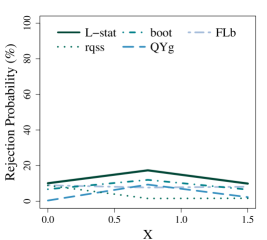
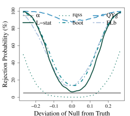
Figure 4: Results from DGP in Model 1 of Fan and Liu (2016), $n=500$, $p=0.5$. Top left: pointwise CP at $x_{0}\in\{0,0.75,1.5\}$, interpolated for visual ease. Top right: pointwise power at the same $x_{0}$ against deviations of $\pm 0.1$. Bottom left: joint power curves. Bottom right: uniform power curves.

Figure 4 (bottom left) shows power curves of the hypothesis tests corresponding to the joint (over $x_{0}\in\{0,0.75,1.5\}$) CIs, varying $H_{0}$ while maintaining the same DGP. The deviations of $Q_{Y|X}(p;x_{0})$ shown on the horizontal axis are the same at each $x_{0}$; zero deviation implies $H_{0}$ is true, in which case the rejection probability is the type I error rate. All methods have good type I error rates: L-stat’s is 6.2%, and other methods’ are below the nominal 5%. L-stat has significantly better power, an advantage of 20–40% at the larger deviations. The bottom right graph in Figure 4 is similar, but based on uniform confidence bands evaluated at $231$ different $x_{0}$. Only L-stat has nearly exact type I error rate and good power.

Next, we use the simulation setup of the rqss vignette in Koenker (2012), which in turn came in part from Ruppert et al. (2003, §17.5.1). Here, $n=400$, $p=0.5$, $d=1$, $\alpha=0.05$, and

$$X_{i}\stackrel{{\scriptstyle iid}}{{\sim}}\textrm{Unif}(0,1),\quad Y_{i}=\sqrt{X_{i}(1-X_{i})}\sin\bigl{(}2\pi(1+2^{-7/5})/(X_{i}+2^{-7/5})\bigr{)}+\sigma(X_{i})U_{i},$$ (16)

where the $U_{i}$ are iid $N(0,1)$, $t_{3}$, Cauchy, or centered $\chi^{2}_{3}$, and $\sigma(X)=0.2$ or $\sigma(X)=0.2(1+X)$. The conditional median function is graphed in the supplemental appendix. Although the function as a whole is not a common shape in economics (with multiple local maxima and minima), it provides insight into different types of functions at different points. For pointwise and joint CIs, we consider 47 equispaced points, $x_{0}=0.04,0.06,\ldots,0.96$; uniform confidence bands are evaluated at 231 equispaced values of $x_{0}$.

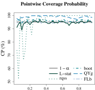
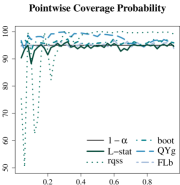
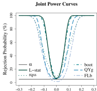
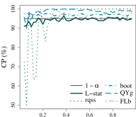
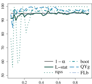
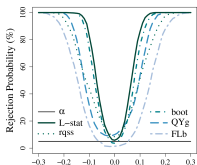
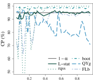
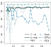
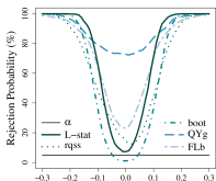
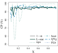
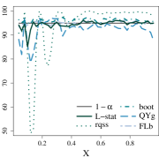
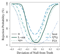
Figure 5: Pointwise CP (first two columns) and joint power curves (third column), $1-\alpha=0.95$, $n=400$, $p=0.5$, DGP in (16). Distributions of $U_{i}$ are, top row to bottom row: $N(0,1)$, $t_{3}$, Cauchy, and centered $\chi^{2}_{3}$. Columns 1 & 3: $\sigma(x)=0.2$; Column 2: $\sigma(x)=(0.2)(1+x)$.

Figure 5’s first two columns show that across all eight DGPs (four error distributions, homoskedastic or heteroskedastic), L-stat has consistently accurate pointwise CP. At the most challenging points (smallest $x_{0}$), L-stat can under-cover by around five percentage points. Otherwise, CP is near $1-\alpha$ for all $x_{0}$ in all DGPs.

In contrast, with the exception of boot, the other methods can have significant under-coverage. As seen in the first two columns of Figure 5, rqss has under-coverage (as low as 50–60% CP) for $x_{0}$ closer to zero. QYg has under-coverage with the $\chi^{2}_{3}$ and (especially) Cauchy. FLb has good CP except with the Cauchy, where CP can dip below 70%.

Figure 5’s third column shows the joint power curves. The horizontal axis of the graphs indicates the deviation of $H_{0}$ from the true values. For example, letting $\xi_{p,j}$ be the true conditional quantiles at the $j=1,\ldots,47$ values of $x_{0}$ (say, $x_{j}$), $-0.1$ deviation refers to $H_{0}:\{Q_{Y|X}(p;x_{j})=\xi_{p,j}-0.1\textrm{ for }j=1,\ldots,47\}$ (which is false), and zero deviation means $H_{0}$ is true. Our method’s type I error rate is close to $\alpha$ under all four $U_{i}$ distributions (5.7%, 5.8%, 7.3%, 6.3%). In contrast, other methods show size distortion under Cauchy and/or $\chi^{2}_{3}$ $U_{i}$; among them, boot is closest but still has $10.3\%$ type I error rate with the $\chi^{2}_{3}$. Next-best is rqss; size distortion for FLb and QYg is more serious. L-stat also has the steepest joint power curves among all methods. Beyond steepness, they are also the most robust to the underlying distribution. L-stat’s type I error rate is near 5% for all four distributions. In contrast, boot ranges from only 1.2% for the Cauchy, leading to worse power, up to 10.3% for the $\chi^{2}_{3}$.

The supplemental appendix shows a comparison of hypothesis tests based on uniform confidence bands. The results are similar to the joint power curves, but with slightly higher rejection rates all around.

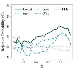
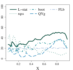
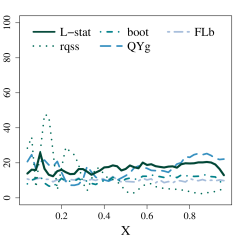
Figure 6: Pointwise power (described in text), $1-\alpha=0.95$, $n=400$, $p=0.5$, DGP from (16), $\sigma(x)=0.2$. The $U_{i}$ are $N(0,1)$ (top left), $t_{3}$ (top right), Cauchy (bottom left), and centered $\chi^{2}_{3}$ (bottom right).

Figure 6 shows pointwise power. Specifically, for a given $x_{0}$, this is the proportion of simulation draws in which $Q_{Y|X}(p;x_{0})-0.1$ is excluded from the CI, averaged with the corresponding proportion for $Q_{Y|X}(p;x_{0})+0.1$. L-stat generally has the best power among methods with correct CP (per first column of Figure 5).

The supplemental appendix contains results for $p=0.25$, where L-stat continues to perform well. One additional advantage is that L-stat’s joint test is nearly unbiased, whereas the other joint tests are all biased.

The supplemental appendix also shows the computational advantage of our method. For example, with $n=10^{5}$ and $100$ different $x_{0}$, L-stat takes only $10$ seconds, whereas the local cubic bootstrap takes $141$ seconds; rqss is even slower.

Overall, the simulation results show the new L-stat method to be fast and accurate. Besides L-stat, the only method to avoid serious under-coverage is the local cubic with bootstrapped standard errors, perhaps due to its reliance on our newly proposed CPE-optimal bandwidth. However, L-stat consistently has better power, greater robustness across different conditional distributions, and less bias of its joint hypothesis tests.

7 Conclusion

We derive a uniform $O(n^{-1})$ difference between the linearly interpolated and ideal fractional order statistic distributions. We generalize this to $L$-statistics to help justify quantile inference procedures. In particular, this translates to $O(n^{-1})$ CPE for the quantile CIs proposed by Hutson (1999), which we improve to $O\mathopen{}\mathclose{{}\left(n^{-3/2}[\log(n)]^{3}}\right)$ via calibration. We extend these results to a nonparametric conditional quantile model, with both theoretical and Monte Carlo success. The derivation of an optimal bandwidth value (not just rate) and a fast approximation thereof are important practical advantages.

Our results can be extended to other objects of interest, such as interquantile ranges and two-sample quantile differences (Goldman and Kaplan, 2016b), quantile marginal effects (Kaplan, 2014), and entire distributions (Goldman and Kaplan, 2016a).

In ongoing work, we consider the connection with Bayesian bootstrap quantile inference, which may be a way to “relax” the iid assumption. Other future work may improve finite-sample performance, e.g., by smoothing over discrete covariates (Li and Racine, 2007).

Appendix A Proof sketches and additional lemmas

The following are only sketches of proofs. The full proofs, with additional intermediate steps and explanations, may be found in the supplemental appendix.

Sketch of proof of Proposition 1

For any $u$, let $k=\lfloor(n+1)u\rfloor$ and $\epsilon=(n+1)u-k\in[0,1)$. If $\epsilon=0$, then the objects $\tilde{Q}^{I}_{X}(u)$, $\hat{Q}^{L}_{X}(u)$, and $F^{-1}\bigl{(}\tilde{Q}^{L}_{U}(u)\bigr{)}$ are identical and equal to $X_{n:k}$. Otherwise, each lies in between $X_{n:k}$ and $X_{n:k+1}$ due to monotonicity of the quantile function and $k/(n+1)\leq u<(k+1)/(n+1)$:

$$X_{n:k} =\tilde{Q}^{I}_{X}\mathopen{}\mathclose{{}\left(k/(n+1)}\right)\leq\tilde{Q}^{I}_{X}(u)\leq\tilde{Q}^{I}_{X}\mathopen{}\mathclose{{}\left((k+1)/(n+1)}\right)=X_{n:k+1},$$

$$X_{n:k} \leq\hat{Q}^{L}_{X}\mathopen{}\mathclose{{}\left(u}\right)=(1-\epsilon)X_{n:k}+\epsilon X_{n:k+1}\leq X_{n:k+1},$$

$$X_{n:k} =F^{-1}\Bigl{(}\tilde{Q}^{L}_{U}\bigl{(}k/(n+1)\bigr{)}\Bigr{)}\leq F^{-1}\Bigl{(}\tilde{Q}^{L}_{U}\mathopen{}\mathclose{{}\left(u}\right)\Bigr{)}\leq F^{-1}\Bigl{(}\tilde{Q}^{L}_{U}\bigl{(}(k+1)/(n+1)\bigr{)}\Bigr{)}=X_{n:k+1}.$$

Thus, differences between the processes can be bounded by the maximum (over $k$) spacing $X_{n:k+1}-X_{n:k}$. Using the assumption that the density is uniformly bounded away from zero over the interval of interest (and applying a maximal inequality from Bickel (1967, eqn. (3.7))), this in turn can be bounded by a maximum of uniform order statistic spacings $U_{n:k+1}-U_{n:k}$. The marginal distribution $(U_{n:k+1}-U_{n:k})\sim\beta(1,n)$ can then be used to bound the probability as needed.

Lemma for PDF approximation

Lemma 7.

Let $\mathbf{\Delta k}$ be a positive $(J+1)$-vector of natural numbers such that $\sum_{j=1}^{J+1}\Delta k_{j}=n+1$, $\min_{j}\{\Delta k_{j}\}\to\infty$, and $\min_{j}\{n-\Delta k_{j}\}\to\infty$, and define $k_{j}\equiv\sum_{i=1}^{j}\Delta k_{i}$ and $\mathbf{k}\equiv(k_{1},\ldots,k_{J})^{\prime}$. Let $\mathbf{X}\equiv(X_{1},\ldots,X_{J})^{\prime}$ be the random $J$-vector such that

$$\mathbf{\Delta X}\equiv(X_{1},X_{2}-X_{1},\ldots,1-X_{J})^{\prime}\sim\textrm{Dirichlet}(\mathbf{\Delta k}).$$

Take any sequence $a_{n}$ that satisfies conditions a) $a_{n}\to\infty$, b) $a_{n}n^{-1}\mathopen{}\mathclose{{}\left[\max\{\Delta k_{j}\}}\right]^{1/2}\to 0$, and c) $a_{n}^{3}\mathopen{}\mathclose{{}\left[\min\{\Delta k_{j}\}}\right]^{-1/2}\to 0$. Define Condition $\star(a_{n})$ as satisfied by vector $\mathbf{x}$ if and only if

$$\max_{j}\mathopen{}\mathclose{{}\left\{n\Delta k_{j}^{-1/2}\mathopen{}\mathclose{{}\left|\Delta x_{j}-\Delta k_{j}/n}\right|}\right\}\leq a_{n}. \star(a_{n})$$ Condition

Let $\|\mathbf{v}\|_{\infty}\equiv\max_{j\in\{1,\ldots,k\}}|v_{j}|$ denote the maximum norm of vector $\mathbf{v}=(v_{1},\ldots,v_{k})^{\prime}$.

1. Condition $\star(a_{n})$ implies

   $$\max_{j}\mathopen{}\mathclose{{}\left\{n\Delta k_{j}^{-1/2}\mathopen{}\mathclose{{}\left|\Delta x_{j}-\Delta k_{j}/(n+1)}\right|}\right\}=O(a_{n}),$$ (17)

   $$\max_{j}\mathopen{}\mathclose{{}\left\{n\Delta k_{j}^{-1/2}\mathopen{}\mathclose{{}\left|\Delta x_{j}-(\Delta k_{j}-1)/(n-J)}\right|}\right\}=O(a_{n}),$$ (18)

   where $\Delta k_{j}/(n+1)$ and $(\Delta k_{j}-1)/(n-J)$ are respectively the mean and mode of $\Delta X_{j}$.

2. At any point of evaluation $\mathbf{\Delta x}$ satisfying Condition $\star(a_{n})$, the log Dirichlet PDF of $\mathbf{\Delta X}$ may be uniformly approximated as

   $$\log f_{\mathbf{\Delta X}}(\mathbf{\Delta x})=D-\frac{(n-J)^{2}}{2}\sum_{j=1}^{J+1}\frac{\mathopen{}\mathclose{{}\left(\Delta x_{j}-\frac{\Delta k_{j}-1}{n-J}}\right)^{2}}{\Delta k_{j}-1}+R_{n},$$

   $$D\equiv\frac{J}{2}\log(n/2\pi)+\frac{1}{2}\sum_{j=1}^{J+1}\log\mathopen{}\mathclose{{}\left(\frac{n}{\Delta k_{j}-1}}\right),$$

   and $R_{n}=O(a_{n}^{3}\|\boldsymbol{\Delta k}^{-1/2}\|_{\infty})$ uniformly (over $\mathbf{\Delta x}$). We also have the uniform (over $\mathbf{\Delta x}$) approximations

   $$\frac{\partial\log[f_{\mathbf{\Delta X}}(\mathbf{\Delta x})]}{\partial\Delta x_{j}} =(n-J)-\frac{(n-J)^{2}}{\Delta k_{j}-1}\mathopen{}\mathclose{{}\left(\Delta x_{j}-\frac{\Delta k_{j}-1}{n-J}}\right)+O(a_{n}^{2}n\|\mathbf{\Delta k}^{-1}\|_{\infty}),$$

   $$\frac{\partial\log[f_{\mathbf{\Delta X}}(\mathbf{x})]}{\partial\Delta k_{j}/n} =-\frac{\partial\log[f_{\mathbf{\Delta X}}(\mathbf{\Delta x})]}{\partial\Delta x_{j}}+O\mathopen{}\mathclose{{}\left(a_{n}^{2}n\|\mathbf{\Delta k}^{-1}\|_{\infty}}\right).$$

3. Uniformly over all $\mathbf{x}\in\mathbb{R}^{J}$ satisfying Condition $\star(a_{n})$,

   $$\log[f_{\mathbf{X}}(\mathbf{x})] =D-\frac{1}{2}(\mathbf{x}-\mathbf{k}/(n+1))^{\prime}\underline{H}(\mathbf{x}-\mathbf{k}/(n+1))+O(a_{n}^{3}\|\mathbf{\Delta k}^{-1/2}\|_{\infty}),$$

   $$\frac{\partial\log[f_{\mathbf{X}}(\mathbf{x})]}{\partial\mathbf{x}} =-\underline{H}(\mathbf{x}-\mathbf{k}/(n+1))+O\mathopen{}\mathclose{{}\left(a_{n}^{2}n\|\mathbf{\Delta k}^{-1}\|_{\infty}}\right),$$

   $$\frac{\partial\log[f_{\mathbf{X}}(\mathbf{x})]}{\partial\mathbf{k}/(n+1)} =\underline{H}(\mathbf{x}-\mathbf{k}/(n+1))+O(a_{n}^{2}n\|\mathbf{\Delta k}^{-1}\|_{\infty}),$$

   where the constant $D$ is the same as in part (ii), and the $J\times J$ matrix $\underline{H}$ has non-zero elements only on the diagonal $\underline{H}_{j,j}=n^{2}\mathopen{}\mathclose{{}\left(\Delta k_{j}^{-1}+\Delta k_{j+1}^{-1}}\right)$ and one off the diagonal $\underline{H}_{j,j+1}=\underline{H}_{j+1,j}=-n^{2}\Delta k_{j+1}^{-1}$. The covariance matrix for $\mathbf{x}$, $\underline{\mathcal{V}}/n\equiv\underline{H}^{-1}$, has row $i$, column $j$ elements

   $$\underline{\mathcal{V}}_{i,j}=\min(k_{i},k_{j})(n+1-\max(k_{i},k_{j}))/[n(n+1)],$$ (19)

   connecting the above with the conventional asymptotic normality results for sample quantiles. That is,

   $$f_{\mathbf{X}}(\mathbf{x}) =\phi_{\underline{\mathcal{V}}/n}\mathopen{}\mathclose{{}\left(\mathbf{x}-\mathbf{k}/(n+1)}\right)\mathopen{}\mathclose{{}\left[1+O\mathopen{}\mathclose{{}\left(a_{n}^{3}\|\mathbf{\Delta k}^{-1/2}\|_{\infty}}\right)}\right],$$ (20)

   $$\frac{\partial f_{\mathbf{X}}(\mathbf{x})}{\partial\mathbf{x}} =\frac{\partial}{\partial\mathbf{x}}\phi_{\underline{\mathcal{V}}/n}\mathopen{}\mathclose{{}\left(\mathbf{x}-\mathbf{k}/(n+1)}\right)+O\mathopen{}\mathclose{{}\left(a_{n}^{4}n^{J/2}n\|\mathbf{\Delta k}^{-1}\|_{\infty}}\right).$$ (21)

4. For the Dirichlet-distributed $\mathbf{\Delta X}$, Condition $\star(a_{n})$ is violated with only exponentially decaying (in $n$) probability: $1-P\bigl{(}\star(a_{n})\bigr{)}=O\bigl{(}a_{n}^{-1}e^{-a_{n}^{2}/2}\bigr{)}.$

5. If instead there are asymptotically fixed components of the parameter vector, the largest of which is $\Delta k_{j}=M<\infty$, then with $M=1$, $1-P\bigl{(}\star(a_{n})\bigr{)}\leq e^{-a_{n}-1}.$ With $M\geq 2$, for any $\eta>0$, $1-P\bigl{(}\star(a_{n})\bigr{)}=o\bigl{(}a_{n}^{-1}\exp\bigl{\{}-a_{n}\sqrt{M}(1/2-\eta)\bigr{\}}\bigr{)}.$

Sketch of proof of Lemma 7

The proof of part (i) uses the triangle inequality and the fact that the mean and mode differ from $\Delta k_{j}/n$ by $O(1/n)$.

For part (ii), since $\mathbf{\Delta X}\sim\textrm{Dirichlet}(\mathbf{\Delta k})$, for any $\mathbf{\Delta x}$ that sums to one,

$$\log(f_{\mathbf{\Delta X}}(\mathbf{\Delta x})) =\log(\Gamma(n+1))+\sum_{j=1}^{J+1}\bigg{[}(\Delta k_{j}-1)\log(\Delta x_{j})-\log(\Gamma(\Delta k_{j}))\bigg{]}.$$ (22)

Applying Stirling-type bounds in Robbins (1955) to the gamma functions,

$$\log(f_{\mathbf{\Delta X}}(\mathbf{\Delta x})) =\overbrace{\frac{J}{2}\log(n/(2\pi))+\frac{1}{2}\sum_{j=1}^{J+1}\log\mathopen{}\mathclose{{}\left(\frac{n}{\Delta k_{j}-1}}\right)}^{D}+\overbrace{\sum_{j=1}^{J+1}(\Delta k_{j}-1)\log\mathopen{}\mathclose{{}\left(\frac{n\Delta x_{j}}{\Delta k_{j}-1}}\right)-J}^{h(\mathbf{\Delta x})}$$

$$\quad+O(\|\mathbf{\Delta k}^{-1}\|_{\infty}),$$ (23)

where $D$ is the same constant as in the statement of the lemma.

We then expand $h(\cdot)$ around the Dirichlet mode, $\mathbf{\Delta x_{0}}$. The cross partials are zero, the first derivative terms sum to zero, and the fourth derivative is smaller-order uniformly over $\mathbf{\Delta x}$ satisfying Condition $\star(a_{n})$:

$$\begin{split}h(\mathbf{\Delta x})&=\overbrace{h(\mathbf{\Delta x_{0}})}^{\equiv R_{1n}=O(n^{-1})}+\sum_{j=1}^{J+1}h_{j}(\mathbf{\Delta x_{0}})(\Delta x_{j}-\Delta x_{0j})+\frac{1}{2}\sum_{j=1}^{J+1}h_{j,j}(\mathbf{\Delta x_{0}})(\Delta x_{j}-\Delta x_{0j})^{2}\\ &\quad+\overbrace{\frac{1}{6}\sum_{j=1}^{J+1}h_{j,j,j}(\mathbf{\Delta x_{0}})(\Delta x_{j}-\Delta x_{0j})^{3}}^{\equiv R_{2n}=O(a_{n}^{3}\|\mathbf{\Delta k}^{-1/2}\|_{\infty})}+\overbrace{\frac{1}{24}\sum_{j=1}^{J+1}h_{j,j,j,j}(\mathbf{\Delta\tilde{x}})(\Delta x_{j}-\Delta x_{0j})^{4}}^{\equiv R_{3n}=O(a_{n}^{4}\|\mathbf{\Delta k}^{-1}\|_{\infty})},\end{split}$$ (24)

where the quadratic term expands to the form in the statement of the lemma.

The derivative with respect to $\mathbf{\Delta x}$ is computed by expanding $h_{j}(\mathbf{\Delta x})=(\Delta k_{j}-1)\Delta x_{j}^{-1}$ around the mode, and then simplifying with Condition $\star(a_{n})$ and the fact that $\sum_{j=1}^{J+1}(\Delta x_{j}-\Delta x_{0,j})=1-1=0$. The derivative with respect to $\Delta k_{j}/n$ is computed from an expansion of $h(\mathbf{\Delta x})$ around the mode, reusing many results from the original computation of the PDF.

For part (iii), the results are intuitive given part (ii), so we defer to the supplemental appendix. It is helpful that the transformation from the values $X_{j}$ to spacings $\Delta X_{j}$ is unimodular.

For part (iv), we use Boole’s inequality along with the beta tail probability bounds from DasGupta (2000) and our beta PDF approximation from Lemma 7(ii).

For part (v), since $\Delta k_{j}=M<\infty$ is a fixed natural number, we can write $\Delta X_{j}=\sum_{i=1}^{M}\delta_{i}$, where each $\delta_{i}$ is a spacing between consecutive uniform order statistics. The marginal distribution of each $\delta_{i}$ is $\beta(1,n)$. Using the corresponding CDF formula and Boole’s inequality leads to the result. The other bound may be derived using equation (6) in Inequality 11.1.1 in Shorack and Wellner (1986, p. 440), as seen in the supplemental appendix, but for our quantile inference application we only use the first result since it is better for $M=1$.

For violations of Condition $\star(a_{n})$ in the other direction, the probability is zero for large enough $n$ since $P(\Delta X_{j}<0)=0$ and $M^{1/2}-a_{n}<0$ for large enough $n$.

Lemma for proving Theorem 2

First, we introduce notation. From earlier, $u_{0}\equiv 0$ and $u_{J+1}\equiv 1$. For all $j$, $k_{j}\equiv\lfloor(n+1)u_{j}\rfloor$, $\epsilon_{j}\equiv(n+1)u_{j}-k_{j}$. Let $\mathbf{\Delta k}$ denote the $(J+1)$-vector such that $\Delta k_{j}=k_{j}-k_{j-1}$, let $\boldsymbol{\psi}=(\psi_{1},\ldots,\psi_{J})^{\prime}$ be the fixed weight vector from (4), and

$$Y_{j} \equiv U_{n:k_{j}}\sim\beta(k_{j},n+1-k_{j}), \mathbf{\Delta Y} \equiv(Y_{1},Y_{2}-Y_{1},\ldots,1-Y_{J})\sim\textrm{Dirichlet}(\mathbf{\Delta k}),$$

$$\Lambda_{j} \equiv U_{n:k_{j}+1}-U_{n:k_{j}}\sim\beta(1,n),$$

$$Z_{j} \equiv\sqrt{n}\mathopen{}\mathclose{{}\left(Y_{j}-u_{j}}\right), V_{j} \equiv\sqrt{n}\mathopen{}\mathclose{{}\left[F^{-1}(Y_{j})-F^{-1}(u_{j})}\right],$$ (25)

$$\mathbb{X} \equiv\sum_{j=1}^{J}\psi_{j}F^{-1}(Y_{j}), \mathbb{X}_{0} \equiv\sum_{j=1}^{J}\psi_{j}F^{-1}(u_{j}),$$

$$\mathbb{W} \equiv\sqrt{n}\mathopen{}\mathclose{{}\left(\mathbb{X}-\mathbb{X}_{0}}\right)=\boldsymbol{\psi}^{\prime}\mathbf{V}, \mathbb{W}_{\boldsymbol{\epsilon},\boldsymbol{\Lambda}}\equiv\mathrlap{\mathbb{W}+n^{1/2}\sum_{j=1}^{J}\epsilon_{j}\psi_{j}\Lambda_{j}\mathopen{}\mathclose{{}\left[Q^{\prime}(u_{j})+Q^{\prime\prime}(u_{j})(Y_{j}-u_{j})}\right],}$$

where the preceding variables are all understood to vary with $n$.

Let $\phi_{\underline{\Sigma}}(\cdot)$ be the PDF of a mean-zero multivariate normal distribution with covariance $\underline{\Sigma}$.

Lemma 8.

1. Let Assumption A2 hold at $\mathbf{\bar{u}}$, and let each element of $\mathbf{Y}$ and $\boldsymbol{\Lambda}$ satisfy Condition $\star(a_{n})$ (as defined in Lemma 7) with $a_{n}=2\log(n)$. The following results hold uniformly over any $\mathbf{u}=\mathbf{\bar{u}}+o(1)$.

2. Let $\mathbf{C}$ be a $J$-vector of random interpolation coefficients as defined in Jones (2002): each $C_{j}\sim\beta(\epsilon_{j},1-\epsilon_{j})$, and they are mutually independent and independent of all other random variables. Then,

   $$\begin{split}\mathopen{}\mathclose{{}\left|n^{1/2}(L^{L}-\mathbb{X}_{0})-\mathbb{W}_{\boldsymbol{\epsilon},\boldsymbol{\Lambda}}}\right|&=O\mathopen{}\mathclose{{}\left(n^{-3/2}[\log(n)]^{3}}\right),\\ \mathopen{}\mathclose{{}\left|n^{1/2}(L^{I}-\mathbb{X}_{0})-\mathbb{W}_{\mathbf{C},\boldsymbol{\Lambda}}}\right|&=O\mathopen{}\mathclose{{}\left(n^{-3/2}[\log(n)]^{3}}\right).\end{split}$$ (26)

3. Define $\underline{\mathcal{V}}$ as the $J\times J$ matrix with row $i$, column $j$ elements $\underline{\mathcal{V}}_{i,j}=\min\{u_{i},u_{j}\}(1-\max\{u_{i},u_{j}\})$, and define $\underline{\mathcal{A}}=\textrm{diag}\{f(F^{-1}(\mathbf{u}))\}$, i.e., $\underline{\mathcal{A}}_{i,j}=f(F^{-1}(u_{i}))$ if $i=j$ and zero if $i\neq j$. Define $\mathcal{V}_{\boldsymbol{\psi}}\equiv\boldsymbol{\psi}^{\prime}\mathopen{}\mathclose{{}\left(\underline{\mathcal{A}}^{-1}\underline{\mathcal{V}}\,\underline{\mathcal{A}}^{-1}}\right)\boldsymbol{\psi}\in\mathbb{R}$. For any realization $\boldsymbol{\lambda}$ of $\boldsymbol{\Lambda}=(\Lambda_{1},\ldots,\Lambda_{J})$ satisfying Condition $\star(2\log(n))$,

   $$\sup_{\{w:\star(2\log(n))\textrm{ holds}\}}\mathopen{}\mathclose{{}\left|\frac{f_{\mathbb{W}_{\mathbb{\epsilon},\boldsymbol{\Lambda}}\mid\boldsymbol{\Lambda}}(w\mid\boldsymbol{\lambda})}{\phi_{\mathcal{V}_{\boldsymbol{\psi}}}(w)}-1}\right|=O\mathopen{}\mathclose{{}\left(n^{-1/2}[\log(n)]^{3}}\right),$$

   $$\sup_{\{w:\star(2\log(n))\textrm{ holds}\}}\mathopen{}\mathclose{{}\left|\frac{\partial f_{\mathbb{W}_{\mathbb{\epsilon},\boldsymbol{\Lambda}}\mid\boldsymbol{\Lambda}}(w\mid\boldsymbol{\lambda})}{\partial w}-\frac{\partial\phi_{\mathcal{V}_{\boldsymbol{\psi}}}(w)}{\partial w}}\right|=O\mathopen{}\mathclose{{}\left(n^{-1/2}[\log(n)]^{3+J}}\right),$$

   where the notation $\phi_{\mathcal{V}_{\boldsymbol{\psi}}}(\cdot)$ denotes the PDF of a normal random variable with mean zero and variance $\mathcal{V}_{\boldsymbol{\psi}}$. For any value $\boldsymbol{\tilde{\epsilon}}\in[0,1)^{J}$, uniformly over $K$ satisfying Condition $\star(a_{n})$,

   $$\mathopen{}\mathclose{{}\left.\frac{\partial^{2}F_{\mathbb{W}_{\boldsymbol{\epsilon},\boldsymbol{\Lambda}}|\boldsymbol{\Lambda}}(K\mid\boldsymbol{\lambda})}{\partial\epsilon_{j}^{2}}}\right|_{\boldsymbol{\epsilon}=\boldsymbol{\tilde{\epsilon}}}=n\psi_{j}^{2}Q^{\prime}(u_{j})^{2}\lambda_{j}^{2}\mathopen{}\mathclose{{}\left[\mathopen{}\mathclose{{}\left.\frac{\partial\phi_{\mathcal{V}_{\boldsymbol{\psi}}}(w)}{\partial w}}\right|_{w=K}}\right]+O\mathopen{}\mathclose{{}\left(n^{-3/2}[\log(n)]^{5+J}}\right).$$

Sketch of proof of Lemma 8

For part (i), with a Taylor expansion, the object $L^{L}$ may be rewritten as

$$L^{L} =\mathbb{X}_{0}+n^{-1/2}\mathbb{W}_{\boldsymbol{\epsilon,\Lambda}}+\sum_{j=1}^{J}\psi_{j}\epsilon_{j}\mathopen{}\mathclose{{}\left(\nu^{L}_{j,1}+\nu_{j,2}^{L}}\right),$$

$$\nu^{L}_{j,1} \equiv\frac{Q^{\prime\prime\prime}(\tilde{u}_{j})}{2}[Y_{j}-u_{j}]^{2}\Lambda_{j},\quad\nu_{j,2}^{L}\equiv\frac{Q^{\prime\prime}(\tilde{y}_{j})}{2}\Lambda_{j}^{2},$$ (27)

where $\forall j$, $\tilde{y}_{j}\in(Y_{j},Y_{j}+\Lambda_{j})$ and $\tilde{u}_{j}$ is between $u_{j}$ and $Y_{j}$. The remainder is $O\bigl{(}n^{-3/2}[\log(n)]^{3}\bigr{)}$ by applying Condition $\star(a_{n})$, noting that A2 uniformly bounds the quantile function derivatives for large enough $n$ under Condition $\star(a_{n})$. The argument for $L^{I}$ is essentially the same.

For part (ii), since $\boldsymbol{\Lambda}$ contains finite spacings, we cannot apply Lemma 7(iii). Instead, we use the result from 8.7.5 in Wilks (1962, p. 238),

$$(\Lambda_{1},\ldots,\Lambda_{J},1-\Lambda_{1}-\cdots-\Lambda_{J})\sim\textrm{Dirichlet}(1,\ldots,1,n+1-J).$$

Directly approximating the corresponding PDF yields

$$\log f_{\boldsymbol{\Lambda}}(\boldsymbol{\lambda}) =J\log(n)-n\sum_{j=1}^{J}\lambda_{j}+O(n^{-1}\log(n)).$$ (28)

For the joint density of $\{\mathbf{Y},\boldsymbol{\Lambda}\}$, define $\mathbf{T}\equiv\bigl{(}\Delta Y_{1},\Lambda_{1},\Delta Y_{2}-\Lambda_{1},\ldots,\Lambda_{J},\Delta Y_{J+1}-\Lambda_{J}\bigr{)}=\underline{T}\bigl{(}\mathbf{Y}^{\prime},\boldsymbol{\Lambda}^{\prime}\bigr{)}^{\prime}$, where $\det(\underline{T})=1$ can be shown. Now

$$\mathbf{T}\sim\textrm{Dirichlet}(\Delta k_{1},1,\Delta k_{2}-1,\ldots,1,\Delta k_{J+1}-1).$$

Using the formula for the PDF of a transformed vector and plugging in the Dirichlet PDF formula for $\mathbf{T}$ yields the joint log PDF of $\mathbf{Y}$ and $\boldsymbol{\Lambda}$. Combining this with the marginal log PDF of $\boldsymbol{\Lambda}$ in (28) yields the log conditional PDF.

For the PDF of $\mathbb{W}$, we can use the formula for the PDF of a transformed random vector and then expand around the $u_{j}$. The transformation from $\mathbf{Z}\equiv Q(\mathbf{Y})$ to $\mathbf{V}\equiv\sqrt{n}\mathopen{}\mathclose{{}\left[Q(\mathbf{Y})-Q(\mathbf{u})}\right]$ (from (25)) is straightforward centering and $\sqrt{n}$-scaling. The last transformation is from $\mathbf{V}$ to $\mathbb{W}=\boldsymbol{\psi}^{\prime}\mathbf{V}$, as defined in (25). For the special case $J=1$, as in our quantile inference application, this step is trivial since $\mathbb{W}=\mathbf{V}$. Altogether, up to this point,

$$f_{\mathbb{W}|\boldsymbol{\Lambda}}(w\mid\boldsymbol{\lambda})=\phi_{\mathcal{V}_{\psi}}(w)\mathopen{}\mathclose{{}\left[1+O\mathopen{}\mathclose{{}\left(n^{-1/2}[\log(n)]^{3}}\right)}\right],$$ (29)

and it remains to account for the difference between $\mathbb{W}$ and $\mathbb{W}_{\boldsymbol{\epsilon},\boldsymbol{\Lambda}}$.

Altogether, it can be shown that the PDF of $\mathbb{W}$ conditional on Condition $\star(a_{n})$ and $\boldsymbol{\Lambda}$ is

$$f_{\mathbb{W}|\star(a_{n}),\boldsymbol{\Lambda}}(w\mid\boldsymbol{\lambda})=\idotsint\limits_{\star(a_{n})}f_{\mathbf{V}|\star(a_{n}),\boldsymbol{\Lambda}}\mathopen{}\mathclose{{}\left(v_{1},\ldots,v_{J-1},\frac{w-\psi_{1}v_{1}-\cdots-\psi_{J-1}v_{J-1}}{\psi_{J}}\mid\boldsymbol{\lambda}}\right)\,dv_{1}\cdots dv_{J-1}.$$

To transition to $\mathbb{W}_{\epsilon,\Lambda}$, define $\eta=\sqrt{n}\sum_{j=1}^{J}\epsilon_{j}\psi_{j}\Lambda_{j}\mathopen{}\mathclose{{}\left[Q^{\prime}(u_{j})+Q^{\prime\prime}(u_{j})(Y_{j}-u_{j})}\right]$, so $\mathbb{W}_{\epsilon,\Lambda}=\mathbb{W}+\eta$. Conditional on $\mathbb{W}=w$, $Y_{1}=y_{1}$, …, $Y_{J-1}=y_{J-1}$, the value of $Y_{J}$ is fully determined. Additionally conditioning on $\boldsymbol{\Lambda}=\boldsymbol{\lambda}$, the value of $\eta$ is fully determined. Along with the implicit function theorem, this can be used to derive the final normal approximation.

Results for the PDF derivative follow the same sequence of transformations; details are left to the supplemental appendix.

For the last result in this part of the lemma, in addition to Condition $\star(2\log(n))$ and A2, we use the law of iterated expectations for CDFs.

Sketch of proof of Theorem 2

For part (i), we start by restricting attention to cases where the largest of the $J$ spacings between relevant uniform order statistics, $U_{n:\lfloor(n+1)u_{j}\rfloor+1}-U_{n:\lfloor(n+1)u_{j}\rfloor}$, and the largest difference between the $U_{n:\lfloor(n+1)u_{j}\rfloor}$ and $u_{j}$ satisfy Condition $\star(2\log(n))$ as in Lemma 7. By Lemma 7(iv,v), the error from this restriction is smaller-order. We then use the representation of ideal uniform fractional order statistics from Jones (2002), which is equal in distribution to the linearly interpolated form but with random interpolation weights $C_{j}\sim\beta(\epsilon_{j},1-\epsilon_{j})$ instead of fixed $\epsilon_{j}$, where each $C_{j}$ is independent of every other random variable we have. The leading term in the error is due to $\operatorname{Var}\mathopen{}\mathclose{{}\left(C_{j}}\right)$, and by plugging in other calculations from Lemma 8, we see that it is uniformly $O(n^{-1})$ and can be calculated analytically.

For part (ii), the first result comes from the FOC

$$0 =\frac{\partial}{\partial K}\frac{K\exp\mathopen{}\mathclose{{}\left\{-K^{2}/(2\mathcal{V}_{\psi})}\right\}}{\sqrt{2\pi\mathcal{V}_{\psi}^{3}}}\mathopen{}\mathclose{{}\left[\sum_{j=1}^{J}\mathopen{}\mathclose{{}\left(\frac{\psi_{j}^{2}\epsilon_{j}(1-\epsilon_{j})}{\mathopen{}\mathclose{{}\left[f\mathopen{}\mathclose{{}\left(F^{-1}\mathopen{}\mathclose{{}\left(u_{j}}\right)}\right)}\right]^{2}}}\right)}\right]n^{-1}$$

whose solution $K=\sqrt{\mathcal{V}_{\psi}}$ is plugged into the expression in Theorem 2(i).

The additional result for $L^{B}$ in part (ii) follows from the Dirichlet PDF approximation in Lemma 8(ii).

Sketch of proof of Lemma 3

The results are based on the Cornish–Fisher-type expansion from Pratt (1968) and Peizer and Pratt (1968), solving for the high-order constants.

Sketch of proof of Theorem 4

For CP, let $R_{n}=O\mathopen{}\mathclose{{}\left(n^{-3/2}[\log(n)]^{3}}\right)$ be the remainder from Theorem 2(i).

For a lower one-sided CI,

$$u^{h}(\alpha) =p+O(n^{-1/2}),\quad J=1,\quad\epsilon_{h}=(n+1)u^{h}(\alpha)-\lfloor(n+1)u^{h}(\alpha)\rfloor,$$

$$\mathcal{V}_{\boldsymbol{\psi}} =\frac{u^{h}(\alpha)(1-u^{h}(\alpha))}{f(F^{-1}(u^{h}(\alpha)))^{2}},\quad\mathbb{X}_{0}=F^{-1}(u^{h}(\alpha)),$$

$$K =n^{1/2}\mathopen{}\mathclose{{}\left[F^{-1}(p)-F^{-1}\mathopen{}\mathclose{{}\left(u^{h}(\alpha)}\right)}\right]=-\frac{z_{1-\alpha}\sqrt{u^{h}(\alpha)(1-u^{h}(\alpha))}}{f(F^{-1}(u^{h}(\alpha)))}+O(n^{-1/2})$$

$$=-z_{1-\alpha}\sqrt{\mathcal{V}_{\psi}}+O(n^{-1/2}),$$

where the first and last lines use Lemma 3, and the last line uses Assumption A2. Then, the rate of coverage probability error is

$$P\mathopen{}\mathclose{{}\left(\hat{Q}^{L}_{X}\mathopen{}\mathclose{{}\left(u^{h}(\alpha)}\right)<Q(p)}\right)=P\mathopen{}\mathclose{{}\left(\hat{Q}^{L}_{X}\mathopen{}\mathclose{{}\left(u^{h}(\alpha)}\right)<\mathbb{X}_{0}+n^{-1/2}K}\right)$$

$$=P\mathopen{}\mathclose{{}\left(\hat{Q}^{I}_{X}\mathopen{}\mathclose{{}\left(u^{h}(\alpha)}\right)<\mathbb{X}_{0}+n^{-1/2}K}\right)+n^{-1}\frac{\epsilon_{h}(1-\epsilon_{h})}{[f(F^{-1}(u^{h}(\alpha)))]^{2}}\frac{K\exp\{-K^{2}/(2\mathcal{V}_{\psi})\}}{\sqrt{2\pi\mathcal{V}_{\psi}^{3}}}+R_{n}$$

$$=\alpha-n^{-1}z_{1-\alpha}\frac{\epsilon_{h}(1-\epsilon_{h})}{p(1-p)}\phi(z_{1-\alpha})+O(n^{-3/2})+R_{n},$$ (30)

where $f(F^{-1}(u^{h}(\alpha)))$ is uniformly (for large enough $n$) bounded away from zero by A2 since $u^{h}(\alpha)=p+O(n^{-1/2})\to p$. The argument for the lower endpoint is similar.

Two-sided CP comes directly from the two one-sided results, replacing $\alpha$ with $\alpha/2$. For the yet-higher-order calibration, the results follow from plugging in the proposed $\tilde{\alpha}$.

The results for power are derived using the normal approximation $\tilde{Q}^{B}_{X}(u)$ of $\hat{Q}^{L}_{X}(u)$, along with a first-order Taylor approximation and arguments that the remainder terms are negligible.

Sketch of proof of Lemma 5

Since the result is similar to other kernel bias results, and since the special case of $d=1$ and $b=2$ is already given in Bhattacharya and Gangopadhyay (1990), we leave the proof to the supplemental appendix and provide only a very brief sketch here. The approach is to start from the definitions of $Q_{Y|X}(p;C_{h})$ and $Q_{Y|X}(p;x)$,

$$p =\int_{C_{h}}\mathopen{}\mathclose{{}\left\{\int_{-\infty}^{Q_{Y|X}(p;C_{h})}f_{Y|X}(y;x)\,dy}\right\}f_{X|C_{h}}(x)\,dx,\quad p=\int_{-\infty}^{Q_{Y|X}(p;x)}f_{Y|X}(y;x)\,dy,\quad\textrm{so}$$

$$0 =\int_{C_{h}}\mathopen{}\mathclose{{}\left\{\int_{Q_{Y|X}(p;x)}^{Q_{Y|X}(p;C_{h})}f_{Y|X}(y;x)\,dy}\right\}f_{X|C_{h}}(x)\,dx.$$

After a change of variables to $w=x/h$, an expansion around $w=0$ is taken, and the bias can be isolated. If $b=2$, $k_{Q}\geq 2$, and $k_{X}\geq 1$, then a second-order expansion is justified; otherwise, the smoothness determines the order of both the expansion and the remainder.

Sketch of proof of Theorem 6

As in Chaudhuri (1991), we consider a deterministic bandwidth sequence, leaving treatment of a random (data-dependent) bandwidth to future work. Whereas $n$ is a deterministic sequence, $N_{n}$ is random, but $N_{n}\stackrel{{\scriptstyle a.s.}}{{\asymp}}nh^{d}$ as shown in Chaudhuri (1991). Another difference with the unconditional case is that the local sample’s distribution, $F_{Y|X}(\cdot;C_{h})$, changes with $n$ (through $h$). The uniformity of the remainder term in Theorem 4 relies on the properties of the PDF in Assumption A2. In the conditional case, we show that these properties hold uniformly over the PDFs $f_{Y|X}(\cdot;C_{h})$ as $h\to 0$, for which we rely on A4, A5, A7, and A8.

In the lower one-sided case, let $\hat{Q}_{Y|C_{h}}^{L}(u_{h})$ be the Hutson (1999) upper endpoint, with notation analogous to Section 2, with $u_{h}=u^{h}(\alpha)$. The CP of the lower one-sided CI is

$$P\mathopen{}\mathclose{{}\left(Q_{Y|X}(p;0)<\hat{Q}_{Y|C_{h}}^{L}(u_{h})}\right) =1-\alpha+\textrm{CPE}_{\textrm{U}}+\textrm{CPE}_{\textrm{Bias}},$$ (31)

where $\textrm{CPE}_{\textrm{U}}$ is CPE due to the unconditional method and $\textrm{CPE}_{\textrm{Bias}}$ comes from the bias:

$$\textrm{CPE}_{\textrm{U}} \equiv P\mathopen{}\mathclose{{}\left(Q_{Y|X}(p;C_{h})<\hat{Q}_{Y|C_{h}}^{L}(u_{h})}\right)-(1-\alpha)=O\mathopen{}\mathclose{{}\left(N_{n}^{-1}}\right),$$

$$\textrm{CPE}_{\textrm{Bias}} \equiv P\mathopen{}\mathclose{{}\left(Q_{Y|X}(p;0)<\hat{Q}_{Y|C_{h}}^{L}(u_{h})}\right)-P\mathopen{}\mathclose{{}\left(Q_{Y|X}(p;C_{h})<\hat{Q}_{Y|C_{h}}^{L}(u_{h})}\right).$$

Using Lemmas 5 and 8, or alternatively Theorem 2, one can show $\textrm{CPE}_{\textrm{Bias}}=O(N_{n}^{1/2}h^{b})$. Then, one can solve for the $h$ that equates the orders of $\textrm{CPE}_{\textrm{U}}$ and $\textrm{CPE}_{\textrm{Bias}}$, i.e., so that $N_{n}^{-1}\asymp N_{n}^{1/2}h^{b}$, using $N_{n}\asymp nh^{d}$.

With two-sided inference, the lower and upper endpoints have opposite bias effects. For the median, the dominant terms of these effects cancel completely. For other quantiles, there is a partial, order-reducing cancellation. The calculations, which use Theorem 2, are extensive and thus left to the supplemental appendix. Ultimately, it can be shown that two-sided CP is $1-\alpha$ plus terms of $O(N_{n}^{-1})$, $O(B_{h})$, and $O(B_{h}^{2}N_{n})$, in addition to smaller-order remainders. With the new CPE terms, one can again solve for the $h$ that sets the orders equal.

References

- Abrevaya (2001) Abrevaya, J. (2001). The effects of demographics and maternal behavior on the distribution of birth outcomes. Empirical Economics 26(1), 247–257.
- Alan et al. (2005) Alan, S., T. F. Crossley, P. Grootendorst, and M. R. Veall (2005). Distributional effects of ‘general population’ prescription drug programs in Canada. Canadian Journal of Economics 38(1), 128–148.
- Andrews and Guggenberger (2014) Andrews, D. W. K. and P. Guggenberger (2014). A conditional-heteroskedasticity-robust confidence interval for the autoregressive parameter. Review of Economics and Statistics 96(2), 376–381.
- Banks et al. (1997) Banks, J., R. Blundell, and A. Lewbel (1997). Quadratic Engel curves and consumer demand. Review of Economics and Statistics 79(4), 527–539.
- Beran and Hall (1993) Beran, R. and P. Hall (1993). Interpolated nonparametric prediction intervals and confidence intervals. Journal of the Royal Statistical Society: Series B (Statistical Methodology) 55(3), 643–652.
- Bhattacharya and Gangopadhyay (1990) Bhattacharya, P. K. and A. K. Gangopadhyay (1990). Kernel and nearest-neighbor estimation of a conditional quantile. Annals of Statistics 18(3), 1400–1415.
- Bickel (1967) Bickel, P. J. (1967). Some contributions to the theory of order statistics. In Proceedings of the Fifth Berkeley Symposium on Mathematical Statistics and Probability, Volume 1: Statistics. The Regents of the University of California.
- Buchinsky (1994) Buchinsky, M. (1994). Changes in the U.S. wage structure 1963–1987: Application of quantile regression. Econometrica 62(2), 405–458.
- Chamberlain (1994) Chamberlain, G. (1994). Quantile regression, censoring, and the structure of wages. In Advances in Econometrics: Sixth World Congress, Volume 2, pp. 171–209.
- Chaudhuri (1991) Chaudhuri, P. (1991). Nonparametric estimates of regression quantiles and their local Bahadur representation. Annals of Statistics 19(2), 760–777.
- Chen and Hall (1993) Chen, S. X. and P. Hall (1993). Smoothed empirical likelihood confidence intervals for quantiles. Annals of Statistics 21(3), 1166–1181.
- DasGupta (2000) DasGupta, A. (2000). Best constants in Chebyshev inequalities with various applications. Metrika 51(3), 185–200.
- David and Nagaraja (2003) David, H. A. and H. N. Nagaraja (2003). Order Statistics (3rd ed.). New York: Wiley.
- Deaton (1997) Deaton, A. (1997). The analysis of household surveys: a microeconometric approach to development policy. Baltimore: The Johns Hopkins University Press.
- Donald et al. (2012) Donald, S. G., Y.-C. Hsu, and G. F. Barrett (2012). Incorporating covariates in the measurement of welfare and inequality: methods and applications. The Econometrics Journal 15(1), C1–C30.
- Engel (1857) Engel, E. (1857). Die productions- und consumtionsverhältnisse des königreichs sachsen. Zeitschrift des Statistischen Bureaus des Königlich Sächsischen, Ministerium des Inneren 8–9, 1–54.
- Fan et al. (2012) Fan, X., I. Grama, and Q. Liu (2012). Hoeffding’s inequality for supermartingales. Stochastic Processes and their Applications 122(10), 3545–3559.
- Fan and Liu (2016) Fan, Y. and R. Liu (2016). A direct approach to inference in nonparametric and semiparametric quantile models. Journal of Econometrics 191(1), 196–216.
- Ferguson (1973) Ferguson, T. S. (1973). A Bayesian analysis of some nonparametric problems. Annals of Statistics 1(2), 209–230.
- Fisher (1932) Fisher, R. A. (1932). Statistical Methods for Research Workers (4th ed.). Edinburg: Oliver and Boyd.
- Goldman and Kaplan (2016a) Goldman, M. and D. M. Kaplan (2016a). Evenly sensitive KS-type inference on distributions. Working paper, available at http://faculty.missouri.edu/~kaplandm.
- Goldman and Kaplan (2016b) Goldman, M. and D. M. Kaplan (2016b). Nonparametric inference on conditional quantile differences, linear combinations, and vectors, using -statistics. Working paper, available at http://faculty.missouri.edu/~kaplandm.
- Hall and Sheather (1988) Hall, P. and S. J. Sheather (1988). On the distribution of a Studentized quantile. Journal of the Royal Statistical Society: Series B (Statistical Methodology) 50(3), 381–391.
- Ho and Lee (2005a) Ho, Y. H. S. and S. M. S. Lee (2005a). Calibrated interpolated confidence intervals for population quantiles. Biometrika 92(1), 234–241.
- Ho and Lee (2005b) Ho, Y. H. S. and S. M. S. Lee (2005b). Iterated smoothed bootstrap confidence intervals for population quantiles. Annals of Statistics 33(1), 437–462.
- Hogg (1975) Hogg, R. (1975). Estimates of percentile regression lines using salary data. Journal of the American Statistical Association 70(349), 56–59.
- Horowitz and Lee (2012) Horowitz, J. L. and S. Lee (2012). Uniform confidence bands for functions estimated nonparametrically with instrumental variables. Journal of Econometrics 168(2), 175–188.
- Hotelling (1939) Hotelling, H. (1939). Tubes and spheres in -space and a class of statistical problems. American Journal of Mathematics 61, 440–460.
- Hutson (1999) Hutson, A. D. (1999). Calculating nonparametric confidence intervals for quantiles using fractional order statistics. Journal of Applied Statistics 26(3), 343–353.
- Jones (2002) Jones, M. C. (2002). On fractional uniform order statistics. Statistics & Probability Letters 58(1), 93–96.
- Kaplan (2014) Kaplan, D. M. (2014). Nonparametric inference on quantile marginal effects. Working paper, available at http://faculty.missouri.edu/~kaplandm.
- Kaplan (2015) Kaplan, D. M. (2015). Improved quantile inference via fixed-smoothing asymptotics and Edgeworth expansion. Journal of Econometrics 185(1), 20–32.
- Kaplan and Sun (2016) Kaplan, D. M. and Y. Sun (2016). Smoothed estimating equations for instrumental variables quantile regression. Econometric Theory XX(XX), XX–XX. Forthcoming.
- Koenker (2012) Koenker, R. (2012). quantreg: Quantile Regression. R package version 4.81.
- Kumaraswamy (1980) Kumaraswamy, P. (1980). A generalized probability density function for double-bounded random processes. Journal of Hydrology 46(1–2), 79–88.
- Lehmann (1951) Lehmann, E. L. (1951). A general concept of unbiasedness. Annals of Mathematical Statistics 22(4), 587–592.
- Li and Racine (2007) Li, Q. and J. S. Racine (2007). Nonparametric econometrics: Theory and practice. Princeton University Press.
- Manning et al. (1995) Manning, W., L. Blumberg, and L. Moulton (1995). The demand for alcohol: the differential response to price. Journal of Health Economics 14(2), 123–148.
- Muir (1960) Muir, T. (1960). A Treatise on the Theory of Determinants. Dover Publications.
- Neyman (1937) Neyman, J. (1937). »Smooth test» for goodness of fit. Skandinavisk Aktuarietidskrift 20(3–4), 149–199.
- Office for National Statistics and Department for Environment, Food and Rural Affairs (2012) Office for National Statistics and Department for Environment, Food and Rural Affairs (2012). Living Costs and Food Survey. 2nd Edition. Colchester, Essex: UK Data Archive. http://dx.doi.org/10.5255/UKDA-SN-7472-2.
- Pearson (1933) Pearson, K. (1933). On a method of determining whether a sample of size n supposed to have been drawn from a parent population having a known probability integral has probably been drawn at random. Biometrika 25, 379–410.
- Peizer and Pratt (1968) Peizer, D. B. and J. W. Pratt (1968). A normal approximation for binomial, , beta, and other common, related tail probabilities, I. Journal of the American Statistical Association 63(324), 1416–1456.
- Polansky and Schucany (1997) Polansky, A. M. and W. R. Schucany (1997). Kernel smoothing to improve bootstrap confidence intervals. Journal of the Royal Statistical Society: Series B (Statistical Methodology) 59(4), 821–838.
- Polonik and Yao (2002) Polonik, W. and Q. Yao (2002). Set-indexed conditional empirical and quantile processes based on dependent data. Journal of Multivariate Analysis 80(2), 234–255.
- Pratt (1968) Pratt, J. W. (1968). A normal approximation for binomial, , beta, and other common, related tail probabilities, II. Journal of the American Statistical Association 63(324), 1457–1483.
- Qu and Yoon (2015) Qu, Z. and J. Yoon (2015). Nonparametric estimation and inference on conditional quantile processes. Journal of Econometrics 185(1), 1–19.
- Rényi (1953) Rényi, A. (1953). On the theory of order statistics. Acta Mathematica Hungarica 4(3), 191–231.
- Robbins (1955) Robbins, H. (1955). A remark on Stirling’s formula. The American Mathematical Monthly 62(1), 26–29.
- Ruppert et al. (2003) Ruppert, D., M. P. Wand, and R. J. Carroll (2003). Semiparametric Regression. Cambridge Series in Statistical and Probabilistic Mathematics. Cambridge University Press.
- Shorack (1972) Shorack, G. R. (1972). Convergence of quantile and spacings processes with applications. Annals of Mathematical Statistics 43(5), 1400–1411.
- Shorack and Wellner (1986) Shorack, G. R. and J. A. Wellner (1986). Empirical Processes with Applications to Statistics. New York: John Wiley & Sons.
- Stigler (1977) Stigler, S. M. (1977). Fractional order statistics, with applications. Journal of the American Statistical Association 72(359), 544–550.
- Thompson (1936) Thompson, W. R. (1936). On confidence ranges for the median and other expectation distributions for populations of unknown distribution form. Annals of Mathematical Statistics 7(3), 122–128.
- Wilks (1962) Wilks, S. S. (1962). Mathematical Statistics. New York: Wiley.