IACHEC¹ Cross-Calibration of Chandra, NuSTAR, Swift, Suzaku, and XMM-Newton with 3C 273 and PKS 2155-304.

Abstract

On behalf of the International Astronomical Consortium for High Energy Calibration (IACHEC), we present results from the cross-calibration campaigns in 2012 on 3C 273 and in 2013 on PKS 2155-304 between the then active X-ray observatories Chandra, NuSTAR, Suzaku, Swift and XMM-Newton. We compare measured fluxes between instrument pairs in two energy bands, 1–5 keV and 3–7 keV and calculate an average cross-normalization constant for each energy range. We review known cross-calibration features and provide a series of tables and figures to be used for evaluating cross-normalization constants obtained from other observations with the above mentioned observatories.

1. Introduction

It is common to have simultaneous or near simultaneous X-ray coverage of astrophysical sources with multiple observations. The community is often faced with the question on how to properly fit joint data sets spanning multiple observatories. It is the mission of the International Astronomical Consortium for High Energy Calibration (IACHEC, Sembay et al. 2010) to provide the proper guidance and cross-calibration information to help the community avoid pitfalls and approach cross-observatory fitting in the correct manner.

Several papers have been published as a result of IACHEC effort, using a variety of methods and targets. Nevalainen et al. (2010); Kettula et al. (2013); Schellenberger et al. (2015) used galaxy clusters to measure the differences in measured temperatures between instruments, and Tsujimoto et al. (2011) used the Pulsar Wind Nebula G21.5-0.9 to measure power-law slopes and fluxes. These studies were focused on extended sources and the differences in measured spectral parameters. For the soft X-ray CCD instruments Plucinsky et al. (2012, 2016) used the supernova remnant 1E 0102.2-7219 to compare the fluxes of the line spectrum, developing an empirical model as a reference spectrum for future cross-calibrations campaigns. For point source flux comparison Ishida et al. (2011) used PKS 2155-304. Furthermore, recent cross-calibration studies have been made by Güver et al. (2016) using simultaneous observations of thermonuclear X-ray bursts from GS 1826-238.

Observatory calibration is under continuing development as instruments age and change. Most calibration updates deal with time dependent changes such as the evolution of instrument gain or contamination, but occasionally errors are discovered and corrected that affect data from the entire mission lifetime. It is therefore necessary to repeat and update cross-calibration campaigns on a regular basis using the newest instrument calibrations available. As instruments get decommissioned and new ones launched, it is also beneficial to the community to relate the newest member to the rest of the group.

We examine in this paper two cross-calibration campaigns conducted in 2012 and 2013 on two sources, the quasar 3C 273, and the BL Lac object PKS 2155-304. Both sources have been used as calibration targets in the past, and they are well suited for several reasons: they are not too bright to cause severe pileup issues for the CCD instruments, their absorbing Galactic column is very low, and the spectra can be well fit by a power-law between 1–20 keV for 3C 273 and 1–10 keV for PKS 2155-304. Both targets are variable so that calibration observations must be simultaneous. In addition, 3C 273 can enter states where it has a curving spectrum above 20 keV, so caution is required for comparing slopes across a wide broadband (Madsen et al. 2015a), and PKS 2155-304 is very soft with $\Gamma\sim 2.7$, so that very long integration times would be required for sufficient statistics above 10 keV.

In this paper we perform two different analyses. First, we find the best fit for each instrument and compare the differences between them, focusing primarily on the flux from which we will derive the cross-calibration constant. Second, we explore the change in flux and cross-normalization constant when we require the same spectral parameters for all data sets, rather than allowing each to take on its best fit. This second situation is what most astronomers do when fitting data from multiple instruments. It is therefore important to understand what systematics one might encounter due to systematic calibration errors that are different among instruments.

The participating instruments were: Chandra with HETGS for 3C 273 and LETGS for PKS 2155-304, NuSTAR, Suzaku with XIS for both targets and HXD-PIN for 3C 273 (there was no detection of the source in GSO), Swift with XRT only (no BAT), and XMM-Newton.

This paper is a summary of the activity of a working group aiming at calibrating the effective areas of different X-ray missions within the framework of the IACHEC. The consortium aims to provide standards for high-energy calibration and to supervise cross calibration between different missions. We refer the readers to the website for more details on IACHEC activity and meetings.

2. The Calibration Targets

2.1. 3C 273

At a redshift of $z=0.158$ (Schmidt 1963), 3C 273 is the nearest high luminosity quasar and has been extensively studied at all wavelengths since its discovery in 1963 (for a review, see Courvoisier 1998). It is characterized as a radio-loud quasar with a jet showing apparent superluminal motion, and 3C 273 exhibits large flux variations across nearly all energies (Soldi et al. 2008).

As observed in many other AGN, there is sometimes a soft excess at low-energy X-rays ($<2$ keV), possibly due to Comptonized UV photons (Page et al. 2004). Above 2 keV and up to $\sim 1$ MeV, previous observations report that the spectrum of 3C 273 is a power-law, as is common for jet-dominated Active Galactic Nuclei (AGN). Over the 30 years that the source has been reliably monitored, there appears to be a long term spectral evolution underlying the short term variations. 3C 273 was in its softest observed state in June 2003 ($\Gamma\sim 1.82\pm 0.01$), a value of $\Delta\Gamma\sim$ 0.3–0.4 above what was measured in the 1980’s ($\Gamma\sim 1.5$). Since then the source has hardened again to a value of $\Gamma\sim 1.6-1.7$ (Chernyakova et al. 2007).

There is evidence of an intermittently weak iron line, which appears to be broad ($\sigma\sim 0.6$ keV, Equivalent Width, EW, $\sim$ 20–60 eV), occasionally neutral (Turner et al. 1990; Page et al. 2004; Grandi & Palumbo 2004) and sometimes ionized (Yaqoob & Serlemitsos 2000; Kataoka et al. 2002). Using the full 244 ks of the NuSTAR observation, of which we here only use the subsection overlapping the other observatories, Madsen et al. (2015a) finds the very weak presence of an iron-line (6.4 keV fixed) with a width and Equivalent Width of $\sigma=0.65\pm 0.03$ keV and $EW=23\pm 11$ eV. Because of the shorter exposure times, it was not detected by the other observatories. The spectrum of 3C 273 during this particular epoch clearly deviated from a power-law above 20 keV and could be fit with a cutoff power-law of $\Gamma=1.627\pm 0.006$ and $E_{\mathrm{cutoff}}=291^{+90}_{-55}$ keV. The interpretation of the turnover is that it is due both to the direct coronal signature of the AGN and reflection off the accretion disk. These components typically are not visible since the jet generally dominates this source above $\sim 20$ keV.

The soft excess was not measurable above 1 keV during the cross-calibration campaign and the turnover was not detectable below 20 keV, so the spectral shape between 1–20 keV is best represented by a power-law.

2.2. PKS 2155-304

PKS 2155-304 is a high-frequency peaked BL Lac (HBL) object at $z=0.116$ and one of the most luminous of its kind. It has been frequently observed at all wavelengths and has consistently shown a soft, $\Gamma>2.5$, X-ray spectrum in the 2–10 keV band (Sembay et al. 1993; Brinkmann et al. 1994; Edelson et al. 1995; Urry et al. 1997; Zhang et al. 1999; Kataoka et al. 2000; Tanihata et al. 2001). Rapid variability can be found on hour time scales in the X-ray and optical bands (Zhang et al. 1999; Edelson et al. 2001; Tanihata et al. 2001; Ishida et al. 2011).

The broadband spectrum of PKS 2155-304 is mostly featureless, but displays two prominent peaks located respectively in the far UV/soft X-ray band and in the GeV band. This double-peaked spectral energy distribution (SED) is believed to originate from synchrotron self-Comptonization (SSC) in which photons are scattered by the energetic electrons in the jet (Band & Grindlay 1985; Ghisellini et al. 1985). The lower energy peak is presumably due to synchrotron emission, and the higher energy, secondary peak in the GeV band from inverse Compton scattering. The turnover into the second peak is believed to occur somewhere between 20 keV and 100 MeV. The broadband SED from X-rays to GeV is typically empirically fitted with a log-parabolic model, but in the narrow energy band we consider (1–10keV), the source has been well described as a power-law (Ishida et al. 2011).

3. Observations and Data Reduction

On 2012 July 17, a cross-calibration campaign was conducted between Chandra, NuSTAR, Suzaku, Swift and XMM-Newton on 3C 273, and for PKS 2155-304 on 2013 April 24. Table 1 lists the observation identification numbers (obsID) and exposure times for the respective observatories. The duration and coverage of each observation is shown schematically in Figure 1. Due to the unfortunate relative beating of South Atlantic Anomaly (SAA) passages and occultation periods between the low Earth orbit observatories (NuSTAR, Suzaku, and Swift), we decided to forego strict simultaneity between all observatories. Instead, we analyze observatory pairs truncated to the overlapping exposures, by only matching the good time intervals (GTIs) of the beginning and end of the overlap.

In this scheme we have 11 observatory pairs (10 for PKS 2155-304 due to the Suzaku/HXD flux being too low) as listed in Table 2. The observation START and STOP times are applied as user GTIs to each pipeline, and the resulting total exposure times for each instrument in a pair are recorded in the last column of the table. Because the occultation/SAA periods are not being excluded, the exposure times are quite different between pairs. However, both sources were relatively stable during the observations as shown in the detailed light curves of Figures 2 and 3, and since the missing exposure times are evenly distributed across the overlapping periods, we determined that it did not impact fitting, since the error of the fit parameters are dominated by the total number of counts, rather than possible short term variations in flux and/or slope. We will discuss the light curves in more detail in Section 4.

3.1. Detailed Reduction and Extraction for each observatory

3.1.1 Chandra

Chandra (Weisskopf et al. 2002) is a single telescope observatory. Its main instrument, the Advanced CCD Imaging Spectrometer (ACIS) is an X-ray imaging-spectrometer consisting of the ACIS-I and ACIS-S CCD arrays. The instrument can be used together with either the High Energy Transmission Gratings (HETGS, Canizares et al. 2005), which has a medium-energy grating (MEG) and a high-energy grating (HEG) arm, or with the Low Energy Transmission Grating (LETG). For these observations the back-side illuminated ACIS-S chip, sensitive in the 0.2–10 keV band, was used.

We reduced the grating spectra using CIAO 4.6.1 and calibration database, CALDB 4.6.1.1 and reprocessed using the CIAO chandra_repro reprocessing script. For 3C 273 the data were taken in grating configuration ACIS+HETG. We computed MEG and HEG spectra, combining the $-1$ and $+1$ orders in both cases. The HEG and MEG spectra were then fit simultaneously in the analysis. For PKS 2155-304 the data were taken with grating configuration ACIS+LETG and we combined orders $-1$ and $+1$.

We used dmextract to create light curves from the 0 order image in 1–3 keV and 3–7 keV bands, binned at a cadence of 5 minutes. In the following, we drop the “ACIS+” abbreviation and simply refer to the instruments as LETGS and HETGS.

3.1.2 NuSTAR

NuSTAR (Harrison et al. 2013) flies two co-aligned conical approximation Wolter-I telescoped coated with Pt/C and W/Si multilayers to provide a broad-band coverage in the hard X-rays between 3–79 keV. The telescopes are focused on the Focal Plane Modules (FPMs) that are CdZnTe crystal hybrid pixel detectors (Kitaguchi et al. 2014) aligned in a 2$\times$2 array. The two modules, FPMA and FPMB, are of identical design.

We reduced the data using nustardas 09Jun15_v1.5.1 and CALDB version 20150904. We used an extraction region of radius 50^′′ for 3C 273 and 40^′′ for PKS 2155-304. Backgrounds were taken on the same detector from a 75^′′ radius circular region, as close to the source as possible without risking contamination. We used nuproducts to extract spectra and all default point source parameters were applied during the pipeline run and in the extraction and generation of response files.

We extracted the light curves using nuproducts and applied PSF and vignetting corrections at 7 keV, since this is where the effective area peaks in the 3–7 keV band. We binned the light curve in 5 minute intervals.

3.1.3 Suzaku

As of the time of writing, Suzaku (Mitsuda et al. 2007) is no longer operational. The observatory consisted of four co-aligned Wolter-I telescopes, aimed at the X-ray Imaging Spectrometer (XIS, Koyama et al. 2007) numbered 0 through 3 and sensitive in the 0.2–12  keV band. XIS2 was not operational during the observations due to micro-meteorite hits. In addition to the XIS, Suzaku also carried the Hard X-ray Detector (HXD) of which the PIN was a component covering the 10–70 keV band. It was a non-imaging detector composed of 64 Si PIN diodes at the bottom of well-type collimators surrounded by GSO anti-coincidence scintillators.

For these observations only 3C 273 was detected by HXD and only in PIN. We will in the following only be discussing HXD-PIN and abbreviate it with HXD.

We reduced the Suzaku data using HEASoft 6.16 and CALDB version 20150105, and reprocessed using the FTOOL aepipeline v1.1.0 reprocessing script. Since the data were taken in 1/4 window mode, extraction regions were chosen by eye to include a 4$\times$8^′ box centered on the sources. Background regions were selected from the remaining exposed area, avoiding point sources identified by eye. Response files were produced using the default parameters using a full ray-tracing simulation from a model point source with the FTOOL sxisimarfgen to create the ARF and properly account for photons lost ($\sim$ 15%) outside of the narrow exposed window.

Light curves were extracted from the same regions with the FTOOL lcurve and binned at a cadence of 5 minutes.

3.1.4 Swift-XRT

Swift (Gehrels et al. 2004) flies a single Wolter-I telescope (XRT) which focuses onto an X-ray CCD device similar to those used by the XMM-Newton/MOS cameras (Burrows et al. 2005). The instrument operates from 0.3–10 keV, and since the primary science goal of Swift is to respond to gamma-ray bursts (GRBs) it operates autonomously to measure GRB light curves and spectra over seven orders of magnitude in flux. To mitigate pile-up, the instrument switches between CCD readout modes depending on the source brightness. Two frequently-used modes are: Windowed Timing (WT) mode, which provides 1D spectral information, and Photon Counting (PC) mode, which allows full 2D imaging-spectroscopy. 3C 273 was observed in PC mode and PKS 2155-304 in WT mode.

We reduced the data using the Swift XRT pipeline swxrtdas 17Jul15_v3.1.1 and CALDB version 20150721. 3C 273 is slightly piled up and we extracted spectra using XSELECT from an annulus of inner radius 16.5^′′and outer radius 71^′′. PKS 2155-304 was not piled up and we extracted a spectrum from a circle of radius 47^′′.

Light curves were extracted from the same regions and binned at a cadence of 5 minutes.

3.1.5 XMM-Newton

XMM-Newton (Jansen et al. 2001) flies three Wolter-I grazing incidence telescopes. Two of the telescopes are each paired with the European Photon Imaging Camera (EPIC) Metal Oxide Semi-conductor CCD arrays (MOS1 and MOS2), and the third with EPIC-pn. All three are sensitive in the 0.15–15 keV band. MOS1 and MOS2 cameras are front-illuminated, and the pn is back-illuminated.

We reduced the data using XMM-Newton Science Analysis System (SAS) version 14.0.0 and Current Calibration Files (CCFs) as of 2015 July 1 starting from ODF level. For event selection we used default values for best spectrum quality. For spectral extractions of both PKS 2155-304 and 3C 273 we excised the inner core with radius of 10^′′ from the EPIC PSFs to avoid possible pile-up effects. For EPIC-pn, we used local backgrounds taken from the corners of the EPIC-pn small window modes, whereas for EPIC-MOS empty sky fields of the peripheral CCDs were used.

Light curves were extracted using the same regions and event selections as in the spectral extraction, binned in 5 minutes intervals, and corrected for effective area, PSF, quantum efficiency, GTI, dead times as well as for background counts using the SAS task epiclccorr.

Table 1Cross calibration campaign

Instrument	obsID	Exposure	obsID	Exposure
		(ks)		(ks)
	3C 273		PKS 2155-304
Chandra	14455	30	15475	30
NuSTAR	10002020001	244	60002022002	45
Swift	00050900019	13	00030795108	17.7
Swift	00050900020	6.9
Suzaku	107013010	39.8	108010010	53.3
XMM-Newton	0414191001	38.9	0411782101	76

Table 2Observatory pairs

GTI Start	GTI Stop	Concatenated	Limiting	Exposure
(MJD)	(MJD)	observation	observation	(ks)
3C 273
56124.346	56125.369	NuSTAR	Suzaku	42.3/40.2
56124.475	56124.822	NuSTAR	Chandra	15.2/29.5
56124.438	56125.389	NuSTAR	Swift	36.3/19.9
56124.504	56124.801	NuSTAR	XMM-Newton	12.8/26.9
56124.475	56124.822	Suzaku	Chandra	13.7/29.5
56124.438	56125.389	Suzaku	Swift	32.7/19.9
56124.504	56124.801	Suzaku	XMM-Newton	10.1/26.9
56124.475	56124.822	Swift	Chandra	7.6/29.5
56124.504	56124.801	Swift	XMM-Newton	7.6/25.3
56124.504	56124.801	Chandra	XMM-Newton	17.8/26.9
PKS 2155-304
56406.184	56406.532	Suzaku	Chandra	8.3/30.1
56405.840	56406.883	Suzaku	NuSTAR	38.4/45.0
56406.146	56406.831	Suzaku	Swift	25.8/17.8
56405.944	56406.808	Suzaku	XMM-Newton	30.7/68.6
56406.184	56406.532	NuSTAR	Chandra	16.0/30.1
56405.840	56406.883	NuSTAR	Swift	29.0/17.8
56405.944	56406.808	NuSTAR	XMM-Newton	31.9/68.6
56406.184	56406.532	XMM-Newton	Chandra	20.9/30.1
56406.146	56406.808	XMM-Newton	Swift	28.9/17.7
56406.184	56406.532	Swift	Chandra	8.1/30.1

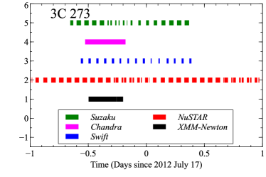
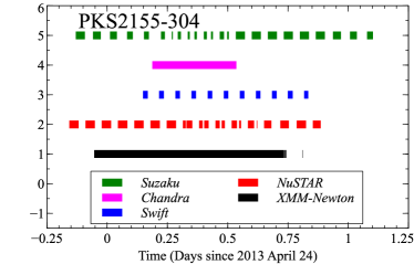
Figure 1.— Observation duration for each observatory for the two cross-calibration campaigns.

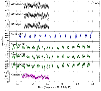
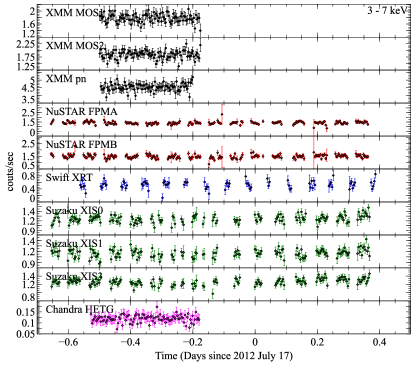
Figure 2.— Light curve of 3C 273 in instrument counts s^-1. See text for instrument specific corrections made to each curve. Bin width is 5 minutes. Large error bars (1$\sigma$) at the edge of the occultation/SAA gaps of the low-Earth orbit instruments are typically due to very small fractional exposures within the bin, or an SAA passage that was not entirely filtered out. The light curves show that there is no rapid variability present.

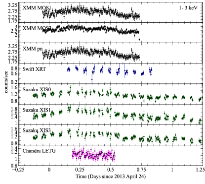
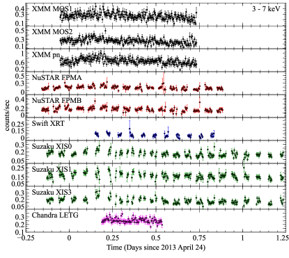
Figure 3.— Same as for Figure 2 but for PKS 2155-304.

3.2. Fitting Procedure

We performed all fits with XSPEC (Arnaud 1996) version 12.8.2 and use Cash C-statistics (Cash 1979) (cstat in XSPEC) as implemented in XSPEC, because of the bias associated with $\chi^{2}$-statistics (Nousek & Shue 1989; Humphrey et al. 2009). A discussion on the benefits of Cash C-statistics and the bias can be found in the XSPEC manual. We ensure that every bin has at least one count, since bins with zero counts can lead to erroneous results in XSPEC. To prove the goodness of fit we binned the spectra after fitting to a minimum of 30 counts and calculated the $\chi_{\mathrm{red}}^{2}$ on the fit obtained with Cash statistics. All errors are 90% confidence unless otherwise stated.

Each observatory, instrument, and source was first fitted independently using an absorbed power-law model, cflux $\times$ tbabs $\times$ pow (in XSPEC). We used Wilms abundances (Wilms et al. 2000) and Verner cross-sections (Verner et al. 1996) and fixed the column to the Galactic values $N_{\rm{H}}$=1.79 $\times 10^{20}$ cm^-2 for 3C 273 and $N_{\rm{H}}$=1.42 $\times 10^{20}$ cm^-2 for PKS2155-304 (Dickey & Lockman 1990). Tests letting $N_{\rm{H}}$ float resulted in inconsistent and unlikely column values ($N_{\rm{H}}$ tended towards 0 for both sources). The value of $N_{\rm{H}}$ is degenerate with slope for the soft instruments and sensitive to their low energy calibration, but allowing the $N_{\rm{H}}$ to vary within previously measured realistic values, revealed that the changes this caused to the slope were smaller than the measurement error on the slope itself. Fixing $N_{\rm{H}}$ to the same value for all observatories therefore introduces minimal biases on slope and flux, mainly because at such low $N_{\rm{H}}$ values the absorption is negligible above $\sim$2 keV, and we do not fit below 1 keV.

We also tested the dependence of the flux and slope for different choices of abundance and/or cross-section, as well as choice of photoelectric absorption model. For abundances we tested Anders & Grevesse (1989) and Lodders & Palme (2009), for cross-sections Balucinska-Church & McCammon (1992), and for photoelectric model tbabs and tbnew. Using the EPIC and XIS spectra as reference, and fitting them in their nominal calibrated energy bandpass, the 3C 273 results are essentially indistinguishable, while the fluxes/slope/column densities from the PKS 2155-304 spectral analysis are minimally affected by less than a fraction of percent, 0.01, and $10^{19}$ cm^-2, respectively.

We applied the XSPEC convolution model cflux to fit the flux instead of the power-law normalization, as this directly gives us the absorbed flux, which is the value we are interested in comparing between instruments. We therefore do not report on the normalization or the intrinsic flux of the power-law.

We use two energy bands for calculating the fitted flux. For the low-energy observatories, Chandra, Suzaku, Swift, and XMM-Newton  we used 1–5 keV when paired with each other, and 3–7 keV when paired with NuSTAR. These energy ranges were chosen for several reasons. First, NuSTAR is not well calibrated below 3 keV, which restricted the lower energy range. Second, to ensure that all spectra were of good quality and well above background, 7 keV was set at the upper limit. Finally, the lower range of 1 keV was picked to avoid complications with detector contamination layers on the CCD instruments. For Suzaku HXD and NuSTAR we used 20–40 keV.

We carefully examined the highest signal to noise observations from Suzaku and XMM-Newton to determine if there is measurable spectral curvature between 1–10 keV in either source. Instead of a simple power-law, we tried fitting with a log-parabolic power-law (logpar) used for blazars, a broken power-law (bknpowlw), and a cutoff power-law (cutpowerlw) used for accretion-dominated sources. The improvements in the fits were not significant for either source. There are changes in the spectral index with different choice in upper and lower energy bound within a single instrument, but the changes are not systematically the same for different observatories and are therefore most likely due to statistical fluctuations or instrument specific calibration.

4. Light Curves

We extracted light curves for all instruments in 5 minute bins for the two non-overlapping energy bands: 1–3 keV (NuSTAR excluded) and 3–7 keV. The light curves are shown in Figures 2 and 3 for the respective bands and two sources. Neither show rapid variability, and the few large outliers, which can be observed adjacent to the occultation/SAA gaps for the low-Earth orbit observatories, are either small fractional flux bins or SAA periods that were not entirely filtered out, and they do not influence the cross-calibration results.

For both sources, the flux follows the same shape in the low and high band with no indication of rapid variability between gaps. We are therefore confident that including the occulted periods for Chandra and XMM-Newton, or between NuSTAR  Suzaku  and Swift  for non-overlapping periods, should not affect the flux measurements.

5. Cross-calibration Results

Tables 3 and 4 summarize the results of the individual fits, and Figures 4 and 5 show the confidence contours (1, 2, and 3$\sigma$) of flux and power-law index of the individual fits to each observatory pair.

The individual fits aim to quantify the question of how different the observatories are from each other. There is some degeneracy between flux and slope and assuming a fixed cross-normalization factor in multi-instrument spectral fitting is therefore not recommended. Rather cross-normalization constants should be allowed to float and their values subsequently evaluated against Tables 6 (1–5 keV) and 6 (3–7 keV and 20–40 keV), which summarize the inter-instrumental and observatory relative flux ratios, and/or in conjunction with Figures 4 and 5. We stress that the ratios are derived from the fluxes in the specific bands as given in Tables 3 and 4, and that they only ensure the flux calculated in this restricted band should agree within reasonable uncertainties between observatories. They do not correct for differences in slope, and deviations may occur if applied outside the specified energy range.

In the individual fits, presented in Tables 6 and 6, the source parameters, $\Gamma$ and flux, between instruments take on different values because of calibration. In many cases, however, a source spectrum can not be constrained by one instrument alone and it is necessary to assume that source parameters are the same for all involved instruments and adjust for the differences between observatories with just one constant (Constant*Model). We show in Figure 6 and 7 the difference in calculated fluxes when tying the model slopes, $\Gamma$, together and when allowing them to take on their optimal value from the individual fits in Tables 3 and 4. Fortunately, there is not much difference in the derived flux, but in the cases where the measured slopes are significantly different, as for Swift/XRT compared to the other instruments, the measured flux of the lowest count rate spectrum gets modified. The exact cross-normalization constant (Constant) between two instruments is therefore sensitive to the relative quality of the spectra, ascribing more influence on the parameters by the higher quality spectrum.

To gain more insight into the observed fluxes and spectral differences between observatories, we calculated fluxes in smaller energy bands tailored to each instrument. For each observatory pair, we used the full valid fitting range for each instrument, but did not go below 1 keV to avoid issues with detector contamination. We then found the best fit to a power-law for the pair leaving all parameters tied and used the model to unfold the spectra and calculate fluxes of the instruments relative to the model. The relative flux ratios for each instrument pair as a function of energy are shown in Figures 8 and 9. There is some uncertainty in the shapes simply due to statistics, but there are a couple of recognizable overall trends that we discuss in detail below.

5.1. Internal Observatory Calibration

In this section we discuss the known features and limitations of the current instrumental calibrations for each observatory respectively.

5.1.1 Chandra

The Chandra HETGS and LETGS effective area calibrations depend on the effective area of the mirror system, the efficiencies of the gratings, the transmission of the ACIS optical blocking filter, the quantum efficiencies of the various ACIS CCDs, and the opacity of the contaminant on the ACIS filter. The contaminant contributes significant uncertainty in the effective area only below 1 keV. The mirror effective area was corrected for an overlayer of static contaminant as of CALDB version 4.1.1 and is estimated to be good to better than 5% above 1 keV. Using in-flight observations of blazars, the HEG and MEG efficiencies were reconciled to better than 3% over the 0.8-5.0 keV range (Marshall 2012), in CALDB version 4.4.6.1. The LETG $\pm 1$ order efficiencies have not been adjusted over the course of the mission but are cross-checked with regular HETGS observations of blazars, agreeing to better than 3%. Absolute calibration is estimated for both the HETGS and LETGS to be at about the 10% level.

5.1.2 NuSTAR

The details on the NuSTAR calibration can be found in Madsen et al. (2015b) and the section below should be regarded as a brief summary.

For PKS 2155-304 FPMA and FPMB fluxes are in agreement and the slopes overlap within errors. For 3C 273 there is a global $\sim 3\%$ offset in flux between the two modules with FPMB being higher than FPMA. This is a known offset, which can be between $\pm 5\%$ and is because the optical axis location on the detector is unique for every observation, but only known absolutely to $\sim 30$^′′. The uncertainty in its location means the vignetting functions could be off by $\sim 30$^′′ and manifests itself as flux offsets and slight slope differences between FPMA/FPMB.

NuSTAR is absolutely calibrated against the Crab assuming a spectrum with $\Gamma=2.1$ and power-law normalization of $N=8.7$ ph $\mathrm{keV^{-1}cm^{-2}s^{-1}}$ at 1 keV. The uncertainty in the absolute value of the slope with respect to chosen $\Gamma$ of the Crab is $\pm 0.01$. This is smaller than the slope uncertainty in either source and the NuSTAR calibration uncertainty therefore does not play into the cross-calibration. The dominant effect is statistical and we note that for PKS 2155-304 the slope for FPMA is systematically harder than FPMB, while for 3C 273 the converse is true and FPMB is harder than FPMA, though still within the uncertainty on the measured values.

5.1.3 Suzaku

The details of the Suzaku XIS and HXD-PIN calibration can be found in a series of memos on the ISAS Suzaku web page and in the Suzaku Technical Description available from the US Suzaku GOF web page. Previous cross-calibration studies have shown that the three sensors of the XIS agree with each other at a 5% level at energies between 1 and 10 keV (Ishida et al. 2011; Tsujimoto et al. 2011). A change in inertial reference units in 2010 produced attitude instability that could cause a source to partially move out of the XIS frame, especially in 1/4 window mode. However, this is properly accounted for in the ray-tracing code that generates the response files (Mitsuda et al. 2007), and the effect on 1–10 keV photometry is well below 5% . Below 1 keV, molecular contamination has greatly reduced the effective area in a way that varies with time, off-axis angle, and XIS (Koyama et al. 2007), however this has no effect in the energy band of the current study. Joint fits between the XIS detectors and the HXD-PIN show that the PIN normalization is about 10% higher than that of the lower energy CCDs.

5.1.4 Swift

The most up-to-date Swift/XRT calibration information can be found on the XRT digest page hosted at the UK Swift Science Data Centre, which summarizes the latest XRT calibration file releases (along with relevant release notes) and highlights any known calibration issues.

Previous comparisons of XRT spectra with data obtained from other instruments (such as XMM-Newton/EPIC, Chandra/ACIS and RXTE/PCA) in general revealed agreements in the power law photon indices to better than $\sim 6$% (i.e. $\Delta\Gamma\lesssim 0.1$) and broadband fluxes to within $\sim 10$%.

We note when analyzing XRT spectra from sources which are piled-up or positioned near the CCD bad-columns, that poorly centered source extraction regions can result in incorrect point spread function correction factors, causing flux inaccuracies at the $\sim$ 5–10% level. Furthermore, as XRT star-tracker derived positions have an associated systematic uncertainty of 3^′′ then extraction regions are best centered for each observation, rather than be based on the expected source coordinates.

High signal-to-noise spectra from sources with featureless continua typically show residuals of about 3%, for example, near the Au-M_V edge (at 2.205 keV), the Si-K edge (at 1.839 keV), or the O-K edge (at 0.545 keV). Occasionally, however, residuals nearer the 10% level are seen, especially near the O-K edge, which are caused by small energy scale offsets (caused by inaccurate bias and/or gain corrections). Such residuals can often be improved through careful use of the gain command in xspec (by allowing the gain offset term to vary by $\sim\pm$10–50 eV).

5.1.5 XMM-Newton

The details on XMM-Newton EPIC calibration can be found in the EPIC calibration status document on the XMM-Newton SOC web page. It is known from previous cross-calibration efforts that EPIC-pn and EPIC-MOS slightly diverge in normalization. We statistically investigated the EPIC cross-calibration using all 23 PKS2155-304 and 21 3C273 observations with all EPIC using small window modes. On average, EPIC-MOS1 (MOS2) return consistently about 5% (7%) higher flux compared to EPIC-pn in the energy range of about 0.5–5 keV. At lower energies, the average flux differences are smaller. At higher energies, the average differences increase to 10-15% in the 5–10 keV band. The average EPIC spectral slopes agree except for the extremes of the sensitivity range. Towards the high end of the band pass (above $\sim 5$ kev), the average EPIC-pn spectral slopes become softer compared to EPIC-MOS, as can be observed in Figures 8 and 9.

5.2. Flux cross-calibration

We have calculated and tabulated the cross-normalization constant between each instrument as measured from the two sources. The constant is the ratio between the derived flux from Tables 3 and 4 for an instrument pair. We stress that the calculated fluxes between instrument pairs that include NuSTAR are for 3–7 keV, all others are for 1–5 keV, except NuSTAR/Suzaku(HXD), which is for 20–40 keV. Table 6 is for the soft instruments only (1–5 keV) while Table 6 is for instrument pairs including NuSTAR (3–7 keV) and Suzaku/HXD (20–40 keV). If a range is shown that means the instrument pair had data for both 3C 273 and PKS 2155-304. If there is only one number, as is the case for the Chandra instruments and Suzaku/HXD, the instrument pair was only active for one of the observations.

There is excellent agreement between Suzaku, Swift/XRT, and XMM-Newton/MOS with only a few percent dispersion. XMM-Newton/pn systematically measures a lower flux with respect to XMM-Newton/MOS, which is a well-known offset and already discussed. Both Chandra/LETGS and HETGS measure a systematically higher flux than all other observatories and is a trend that has been noted before in other studies (Nevalainen et al. 2010; Tsujimoto et al. 2011). In the harder band, 3-7 keV, which is together with NuSTAR, there is excellent agreement between Swift/XRT, XMM-Newton/MOS and Suzaku/XIS0 and XIS3, while XIS1 measures a few percent lower values than the other instruments. Suzaku/HXD has about 10% higher flux than NuSTAR in the 20–40 keV band, which was expected from the XIS/PIN internal relative normalizations.

5.3. Cross-observatory spectral discrepancies

As can be seen from Figures 8 and 9 these cross-normalization constants may change with a different choice of overlapping energy band. Caution must be urged, though, not to read too much into features such as the convex trend observed in Suzaku XIS instruments in PKS 2155-304, which is not repeated for 3C 273. For a feature to be called systematic, it should be observed in several independent observations and for different targets, and the non-repeated differences between instruments should instead be regarded as an indication of the magnitude of statistical fluctuations that might occur.

A trend that does repeat and has been observed in other cross-calibration papers, is the harder spectrum derived from LETGS and higher overall flux peaking at around $\sim$3–4 keV with respect to Suzaku/XIS and XMM-Newton/MOS (see Figure 9, Ishida et al. 2011). Likewise, for both sources Swift/XRT shows a harder spectrum, and the XRT flux is typically less than other instruments below $\sim$3 keV and higher above. The shallower slope is similar to Chandra, which has been confirmed also for G21.5-0.9 (Tsujimoto et al. 2011), where a new analysis with updated response files finds agreement between the two instruments^,. For Chandra the flux below 3 keV is in agreement with XMM-Newton/MOS and Suzaku/XIS, but rises to a peak of 10–15% above 4 keV with respect to the other instruments.

For these two sources, XMM-Newton shows a harder spectrum above 3 keV with respect to Suzaku, but this is not always the case as shown in Ishida et al. (2011) where several observations of PKS 2155-304 were investigated. As already stated, pn measures a flux that is 5% below that of MOS for energies less than 5 keV. Above 5 keV the difference in flux between pn and MOS increases to 10–15%, which is the result of a softer pn slope.

There is good agreement between the measured slope of Suzaku/HXD and NuSTAR, but with a 10% difference in flux. The statistical level of the overlapping energy bands of NuSTAR with the soft instruments is not high enough to reveal any systematic trends. By design, the average NuSTAR flux was set to be roughly between the other observatories.

Table 3Cross-calibration cflux $\times$ tbabs $\times$ pow

Instrument	$\Gamma$	Flux 3–7 keV	$\chi^{2}_{\mathrm{red}}$
		$10^{-12}$ erg cm-2 s-1
3C 273
NuSTAR FPMA	1.54 $\pm$0.06	40.1 $\pm$0.62	1.079
NuSTAR FPMB	1.65 $\pm$0.06	42.0 $\pm$0.67	0.673
Chandra HETGS	1.61 $\pm$0.07	44.8 $\pm$0.85	0.479
NuSTAR FPMA	1.59 $\pm$0.04	41.0 $\pm$0.38	1.052
NuSTAR FPMB	1.63 $\pm$0.04	43.1 $\pm$0.40	0.970
Suzaku XIS0	1.61 $\pm$0.03	40.9 $\pm$0.31	1.040
Suzaku XIS1	1.68 $\pm$0.03	39.6 $\pm$0.31	0.929
Suzaku XIS3	1.68 $\pm$0.03	40.6 $\pm$0.30	1.089
NuSTAR FPMA	1.59 $\pm$0.04	41.0 $\pm$0.42	1.069
NuSTAR FPMB	1.63 $\pm$0.04	42.8 $\pm$0.21	0.936
Swift XRT	1.40 $\pm$0.15	45.4 $\pm$1.77	0.692
NuSTAR FPMA	1.55 $\pm$0.07	39.7 $\pm$0.68	1.085
NuSTAR FPMB	1.64 $\pm$0.07	41.9 $\pm$0.35	0.742
XMM-Newton MOS1	1.45 $\pm$0.06	42.0 $\pm$0.61	1.022
XMM-Newton MOS2	1.43 $\pm$0.06	42.1 $\pm$0.59	0.993
XMM-Newton pn	1.65 $\pm$0.05	36.0 $\pm$0.46	1.037
Instrument	$\Gamma$	Flux 1–5 keV	$\chi^{2}_{\mathrm{red}}$
		$10^{-12}$ erg cm-2 s-1
Suzaku XIS0	1.64 $\pm$0.01	58.8 $\pm$0.47	0.993
Suzaku XIS1	1.69 $\pm$0.01	57.3 $\pm$0.41	1.065
Suzaku XIS3	1.65 $\pm$0.01	57.9 $\pm$0.45	0.999
Chandra HETGS	1.58 $\pm$0.01	63.5 $\pm$0.57	0.530
Suzaku XIS0	1.64 $\pm$0.01	59.5 $\pm$0.30	0.973
Suzaku XIS1	1.66 $\pm$0.01	58.5 $\pm$0.31	1.046
Suzaku XIS3	1.63 $\pm$0.01	58.7 $\pm$0.29	0.977
Swift XRT	1.48 $\pm$0.04	61.2 $\pm$1.39	1.056
Suzaku XIS0	1.64 $\pm$0.02	57.9 $\pm$0.56	0.968
Suzaku XIS1	1.68 $\pm$0.00	57.0 $\pm$0.52	1.136
Suzaku XIS3	1.65 $\pm$0.02	57.5 $\pm$0.51	1.004
XMM-Newton MOS1	1.66 $\pm$0.01	58.8 $\pm$0.47	1.149
XMM-Newton MOS2	1.67 $\pm$0.01	59.3 $\pm$0.46	1.066
XMM-Newton pn	1.69 $\pm$0.01	53.9 $\pm$0.34	1.061
Swift XRT	1.46 $\pm$0.07	58.8 $\pm$2.13	1.524
Chandra HETGS	1.58 $\pm$0.01	63.5 $\pm$0.57	0.530
XMM-Newton MOS1	1.66 $\pm$0.01	58.8 $\pm$0.47	1.149
XMM-Newton MOS2	1.67 $\pm$0.01	59.3 $\pm$0.46	1.066
XMM-Newton pn	1.69 $\pm$0.01	53.9 $\pm$0.34	1.061
Chandra HETGS	1.58 $\pm$0.01	63.4 $\pm$0.60	0.487
Swift XRT	1.46 $\pm$0.07	58.8 $\pm$2.13	1.548
XMM-Newton MOS1	1.66 $\pm$0.01	58.8 $\pm$0.47	1.149
XMM-Newton MOS2	1.67 $\pm$0.01	59.3 $\pm$0.46	1.066
XMM-Newton pn	1.69 $\pm$0.01	53.9 $\pm$0.34	1.061
Instrument	$\Gamma$	Flux 20–40 keV	$\chi^{2}_{\mathrm{red}}$
		$10^{-12}$ erg cm-2 s-1
NuSTAR FPMA	1.76 $\pm$0.06	60.3 $\pm$1.50	1.023
NuSTAR FPMB	1.85 $\pm$0.06	61.4 $\pm$1.59	0.978
Suzaku HXD	1.77 $\pm$0.10	68.0 $\pm$3.27	0.860

Table 4Cross-calibration cflux $\times$ tbabs $\times$ pow

Instrument	$\Gamma$	Flux 3–7 keV	$\chi^{2}_{\mathrm{red}}$
		$10^{-12}$ erg cm-2 s-1
PKS2155-304
NuSTAR FPMA	2.76 $\pm$0.20	5.88 $\pm$0.27	0.768
NuSTAR FPMB	2.65 $\pm$0.20	5.79 $\pm$0.14	1.089
Chandra ACIS LETGS	3.08 $\pm$0.21	6.42 $\pm$0.27	0.456
NuSTAR FPMA	2.85 $\pm$0.09	5.55 $\pm$0.18	0.974
NuSTAR FPMB	2.76 $\pm$0.10	5.44 $\pm$0.13	1.067
Suzaku XIS0	2.98 $\pm$0.11	4.99 $\pm$0.12	1.116
Suzaku XIS1	3.07 $\pm$0.12	4.80 $\pm$0.12	0.924
Suzaku XIS3	2.95 $\pm$0.10	5.19 $\pm$0.12	0.966
NuSTAR FPMA	2.89 $\pm$0.15	5.40 $\pm$0.19	0.909
NuSTAR FPMB	2.72 $\pm$0.16	5.43 $\pm$0.20	1.211
Swift XRT	2.94 $\pm$0.26	5.45 $\pm$0.28	1.261
NuSTAR FPMA	2.83 $\pm$0.13	5.57 $\pm$0.17	0.950
NuSTAR FPMB	2.78 $\pm$0.13	5.64 $\pm$0.18	1.240
XMM-Newton MOS1	2.64 $\pm$0.09	5.66 $\pm$0.11	1.056
XMM-Newton MOS2	2.68 $\pm$0.09	5.41 $\pm$0.11	0.895
XMM-Newton pn	2.77 $\pm$0.07	5.06 $\pm$0.09	1.047
Instrument	$\Gamma$	Flux 1–5 keV	$\chi^{2}_{\mathrm{red}}$
		$10^{-12}$ erg cm-2 s-1
Suzaku XIS0	2.91 $\pm$0.04	19.1 $\pm$0.36	1.192
Suzaku XIS1	2.82 $\pm$0.04	20.0 $\pm$0.32	1.095
Suzaku XIS3	2.79 $\pm$0.04	20.0 $\pm$0.34	0.907
Chandra ACIS LETGS	2.61 $\pm$0.03	22.1 $\pm$0.31	0.587
Suzaku XIS0	2.81 $\pm$0.02	18.0 $\pm$0.18	1.187
Suzaku XIS1	2.80 $\pm$0.02	18.4 $\pm$0.17	1.058
Suzaku XIS3	2.76 $\pm$0.02	18.4 $\pm$0.16	0.953
Swift XRT	2.64 $\pm$0.04	18.2 $\pm$0.31	1.099
Swift XRT	2.62 $\pm$0.06	19.6 $\pm$0.49	1.145
Chandra ACIS LETGS	2.61 $\pm$0.03	22.1 $\pm$0.31	0.587
Suzaku XIS0	2.80 $\pm$0.02	18.6 $\pm$0.17	1.215
Suzaku XIS1	2.78 $\pm$0.02	19.0 $\pm$0.16	1.128
Suzaku IS3	2.74 $\pm$0.02	19.0 $\pm$0.15	0.988
XMM-Newton MOS1	2.79 $\pm$0.01	18.8 $\pm$0.06	1.086
XMM-Newton MOS2	2.82 $\pm$0.01	18.8 $\pm$0.12	0.947
XMM-Newton pn	2.76 $\pm$0.01	18.0 $\pm$0.08	1.077
XMM-Newton MOS1	2.80 $\pm$0.02	19.7 $\pm$0.19	1.099
XMM-Newton MOS2	2.82 $\pm$0.02	19.6 $\pm$0.18	1.012
XMM-Newton pn	2.77 $\pm$0.01	18.7 $\pm$0.15	1.020
Chandra ACIS LETGS	2.61 $\pm$0.03	22.1 $\pm$0.31	0.587
Swift XRT	2.64 $\pm$0.04	18.2 $\pm$0.31	1.099
XMM-Newton MOS1	2.81 $\pm$0.01	18.8 $\pm$0.14	1.080
XMM-Newton MOS2	2.84 $\pm$0.01	18.7 $\pm$0.13	1.051
XMM-Newton pn	2.78 $\pm$0.01	17.9 $\pm$0.12	0.957

Table 5Cross normalization constants (1-5 keV)

Top/Bottom	LETGS	HETGS	XIS0	XIS1	XIS3	XRT	MOS1	MOS2	pn
LETGS	1	-	$0.87(2)$	$0.90(1)$	$0.91(2)$	$0.89(2)$	$0.89(1)$	$0.89(1)$	$0.85(1)$
HETGS	-	1	$0.93(1)$	$0.90(1)$	$0.91(1)$	$0.93(3)$	$0.93(1)$	$0.94(1)$	$0.85(0)$
XIS0	$1.15(2)$	$1.08(1)$	1	$0.96(3)-0.97(1)$	$0.99(1)-1.04(3)$	$1.02(2)-1.03(2)$	$1.01(1)-1.01(1)$	$1.01(1)-1.02(1)$	$0.93(1)-0.97(1)$
XIS1	$1.11(2)$	$1.08(1)$	$1.03(1)-1.04(3)$	1	$1.03(1)-1.08(3)$	$0.99(1)-1.05(2)$	$0.99(0)-1.03(1)$	$0.99(1)-1.04(1)$	$0.95(1)-0.95(0)$
XIS3	$1.10(2)$	$1.08(1)$	$0.96(3)-1.01(1)$	$0.92(3)-0.98(1)$	1	$0.99(1)-1.04(2)$	$0.99(0)-1.02(1)$	$0.99(1)-1.03(1)$	$0.94(1)-0.95(0)$
XRT	$1.12(3)$	$1.08(4)$	$0.97(2)-0.98(1)$	$0.95(2)-1.01(1)$	$0.96(2)-1.01(1)$	1	$1.00(3)-1.03(1)$	$1.01(3)-1.03(1)$	$0.92(3)-0.98(1)$
MOS1	$1.12(1)$	$1.08(1)$	$0.99(1)-0.99(0)$	$0.97(1)-1.01(0)$	$0.98(1)-1.01(0)$	$0.97(1)-1.00(3)$	1	$0.96(2)-1.00(2)$	$0.86(1)-0.89(2)$
MOS2	$1.12(1)$	$1.07(1)$	$0.98(1)-0.99(1)$	$0.96(1)-1.01(1)$	$0.97(1)-1.01(1)$	$0.97(1)-0.99(3)$	$1.00(2)-1.05(3)$	1	$0.86(1)-0.93(2)$
pn	$1.18(1)$	$1.17(1)$	$1.03(1)-1.07(1)$	$1.05(1)-1.06(1)$	$1.06(1)-1.07(1)$	$1.02(1)-1.09(4)$	$1.12(3)-1.17(2)$	$1.07(2)-1.17(2)$	1

Note - cross-normalization constants from Table 3 and 4. Where a range is given the instrument observed both sources, and the range are directly the lower and higher ratio.

Table 6Cross normalization constants (3-7 keV & 20-40 keV)

Top/Bottom	LETGS	HETGS	FPMA&FPMB	XIS0	XIS1	XIS3	HXD	XRT	MOS1	MOS2	pn
FPMA & FPMB	$1.09(3)$	$1.10(7)$	1	$0.91(4)-0.97(1)$	$0.87(4)-0.94(1)$	$0.95(4)-0.97(1)$	$1.12(6)$	$1.01(7)-1.08(4)$	$1.01(5)-1.03(2)$	$0.97(4)-1.03(2)$	$0.88(2)-0.90(4)$

Note - cross-normalization constants from Table 3 and 4. Where a range is given the instrument observed both sources, and the range are directly the lower and higher ratio.

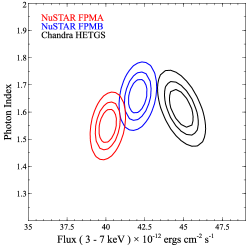
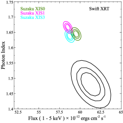
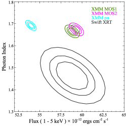
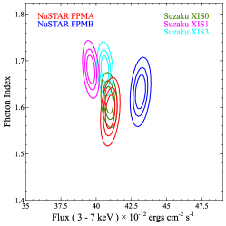
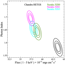
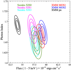
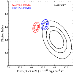
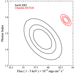
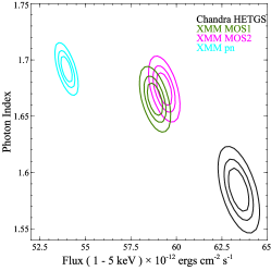
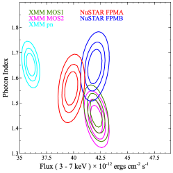
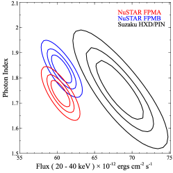
Figure 4.— Confidence contours for 3C 273. The flux axes for the two energy bands 1–5 keV and 3–7 keV have been aligned, but not for the slope axis, $\Gamma$.

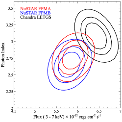
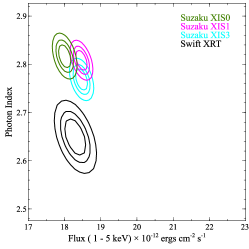
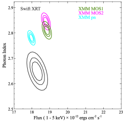
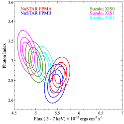
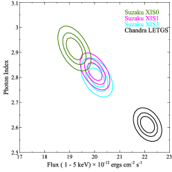
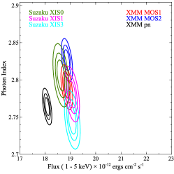
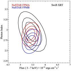
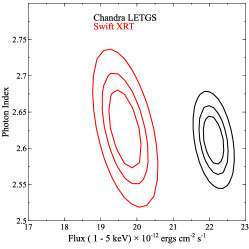
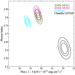
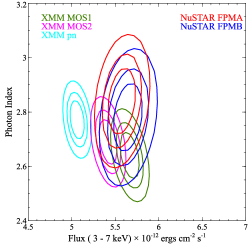
Figure 5.— Confidence contours for PKS2155-304. The flux axes for the two energy bands 1–5 keV and 3–7 keV have been aligned, but not for the slope axis, $\Gamma$.

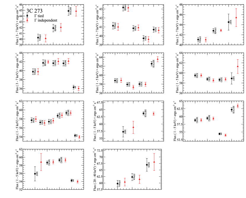
Figure 6.— Flux comparison between instruments when the slope, $\Gamma$, is tied (black circles) and left free to fit independently (red triangles) for 3C 273. In most cases the measured flux is the same within errors, but the spectrum with the lowest statistics does run a risk of being modified by the high statistic spectrum.

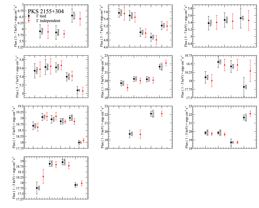
Figure 7.— Flux comparison between instruments when the slope, $\Gamma$, is tied (black circles) and left free to fit independently (red triangles) for PKS 2155-304. In most cases the measured flux is the same within errors, but the spectrum with the lowest statistics does run a risk of being modified by the high statistic spectrum.

6. Conclusion

We have calculated flux ratios between the five observatories Chandra, NuSTAR, Suzaku, Swift, and XMM-Newton for restricted energy bands 1–5 keV, 3–7 keV for those involving NuSTAR, and 20–40 keV for NuSTAR and Suzaku/HXD. We stress that the cross-normalization constants derived from the fluxes are valid only in the specified energy bands, and do not inform on the differences in spectral slopes between instruments. Results from multiple observatories should be judiciously evaluated against the information provided in this paper, and it should be understood that in the absence of an absolute calibration source there is no instrument that is more “correct” than the other.

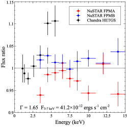
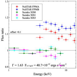
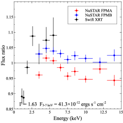
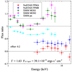
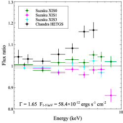
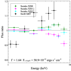
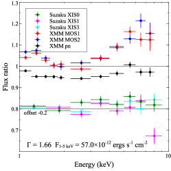
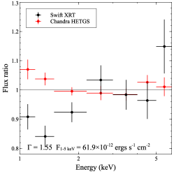
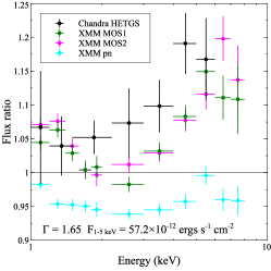
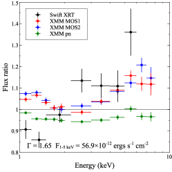
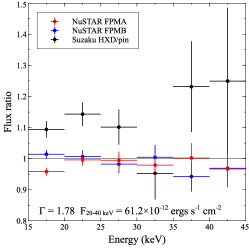
Figure 8.— Flux ratios for 3C273. The offset lines are for viewing purposes only.

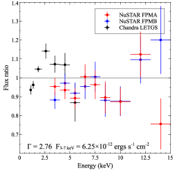
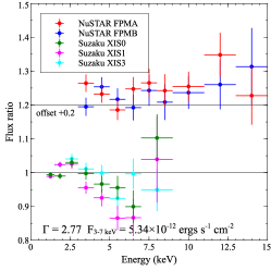
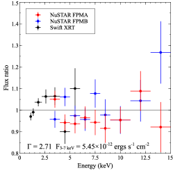
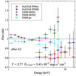
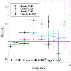
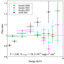
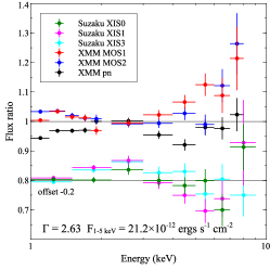
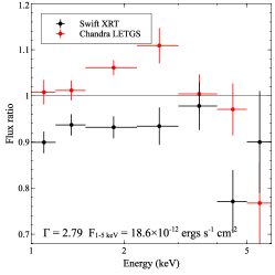
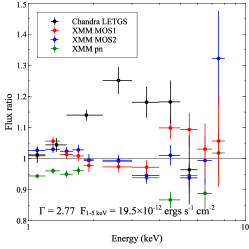
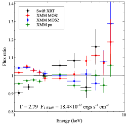
Figure 9.— Flux ratios for PKS2155-304. The offset lines are for viewing purposes only.

References

- Anders & Grevesse (1989) Anders E., Grevesse N., 1989, Geochim. Cosmochim. Acta53, 197
- Arnaud (1996) Arnaud K.A., 1996, In: Jacoby G.H., Barnes J. (eds.) Astronomical Data Analysis Software and Systems V, Vol. 101. Astronomical Society of the Pacific Conference Series, p. 17
- Balucinska-Church & McCammon (1992) Balucinska-Church M., McCammon D., 1992, ApJ400, 699
- Band & Grindlay (1985) Band D.L., Grindlay J.E., 1985, ApJ298, 128
- Brinkmann et al. (1994) Brinkmann W., Maraschi L., Treves A., et al., 1994, A&A288, 433
- Burrows et al. (2005) Burrows D.N., Hill J.E., Nousek J.A., et al., 2005, Space Sci. Rev.120, 165
- Canizares et al. (2005) Canizares C.R., Davis J.E., Dewey D., et al., 2005, PASP117, 1144
- Cash (1979) Cash W., 1979, ApJ228, 939
- Chernyakova et al. (2007) Chernyakova M., Neronov A., Courvoisier T.J.L., et al., 2007, A&A465, 147
- Courvoisier (1998) Courvoisier T.J.L., 1998, A&A Rev.9, 1
- Dickey & Lockman (1990) Dickey J.M., Lockman F.J., 1990, ARA&A28, 215
- Edelson et al. (2001) Edelson R., Griffiths G., Markowitz A., et al., 2001, ApJ554, 274
- Edelson et al. (1995) Edelson R., Krolik J., Madejski G., et al., 1995, ApJ438, 120
- Gehrels et al. (2004) Gehrels N., Chincarini G., Giommi P., et al., 2004, ApJ611, 1005
- Ghisellini et al. (1985) Ghisellini G., Maraschi L., Treves A., 1985, A&A146, 204
- Grandi & Palumbo (2004) Grandi P., Palumbo G.G.C., 2004, Science 306, 998
- Güver et al. (2016) Güver T., Özel F., Marshall H., et al., 2016, ApJ829, 48
- Harrison et al. (2013) Harrison F.A., Craig W.W., Christensen F.E., et al., 2013, ApJ770, 103
- Humphrey et al. (2009) Humphrey P.J., Liu W., Buote D.A., 2009, ApJ693, 822
- Ishida et al. (2011) Ishida M., Tsujimoto M., Kohmura T., et al., 2011, PASJ63, 657
- Jansen et al. (2001) Jansen F., Lumb D., Altieri B., et al., 2001, A&A365, L1
- Kataoka et al. (2000) Kataoka J., Takahashi T., Makino F., et al., 2000, ApJ528, 243
- Kataoka et al. (2002) Kataoka J., Tanihata C., Kawai N., et al., 2002, MNRAS336, 932
- Kettula et al. (2013) Kettula K., Nevalainen J., Miller E.D., 2013, A&A552, A47
- Kitaguchi et al. (2014) Kitaguchi T., Bhalerao V., Cook W.R., et al., 2014, In: Society of Photo-Optical Instrumentation Engineers (SPIE) Conference Series, Vol. 9144. Society of Photo-Optical Instrumentation Engineers (SPIE) Conference Series, p. 91441R
- Koyama et al. (2007) Koyama K., Tsunemi H., Dotani T., et al., 2007, PASJ59, 23
- Lodders & Palme (2009) Lodders K., Palme H., 2009, Meteoritics and Planetary Science Supplement 72, 5154
- Madsen et al. (2015a) Madsen K.K., Fürst F., Walton D.J., et al., 2015a, ApJ812, 14
- Madsen et al. (2015b) Madsen K.K., Harrison F.A., Markwardt C.B., et al., 2015b, ApJS220, 8
- Marshall (2012) Marshall H.L., 2012, In: Society of Photo-Optical Instrumentation Engineers (SPIE) Conference Series, Vol. 8443. Society of Photo-Optical Instrumentation Engineers (SPIE) Conference Series, p. 48
- Mitsuda et al. (2007) Mitsuda K., Bautz M., Inoue H., et al., 2007, PASJ59, 1
- Nevalainen et al. (2010) Nevalainen J., David L., Guainazzi M., 2010, A&A523, A22
- Nousek & Shue (1989) Nousek J.A., Shue D.R., 1989, ApJ342, 1207
- Page et al. (2004) Page K.L., Turner M.J.L., Done C., et al., 2004, MNRAS349, 57
- Plucinsky et al. (2012) Plucinsky P.P., Beardmore A.P., DePasquale J.M., et al., 2012, In: Space Telescopes and Instrumentation 2012: Ultraviolet to Gamma Ray, Vol. 8443. Proc. SPIE, p. 844312
- Plucinsky et al. (2016) Plucinsky P.P., Beardmore A.P., Foster A., et al., 2016, ArXiv e-prints
- Schellenberger et al. (2015) Schellenberger G., Reiprich T.H., Lovisari L., et al., 2015, A&A575, A30
- Schmidt (1963) Schmidt M., 1963, Nature197, 1040
- Sembay et al. (2010) Sembay S., Guainazzi M., Plucinsky P., Nevalainen J., 2010, X-ray Astronomy 2009; Present Status, Multi-Wavelength Approach and Future Perspectives 1248, 593
- Sembay et al. (1993) Sembay S., Warwick R.S., Urry C.M., et al., 1993, ApJ404, 112
- Soldi et al. (2008) Soldi S., Türler M., Paltani S., et al., 2008, A&A486, 411
- Tanihata et al. (2001) Tanihata C., Urry C.M., Takahashi T., et al., 2001, ApJ563, 569
- Tsujimoto et al. (2011) Tsujimoto M., Guainazzi M., Plucinsky P.P., et al., 2011, A&A525, A25
- Turner et al. (1990) Turner M.J.L., Williams O.R., Courvoisier T.J.L., et al., 1990, MNRAS244, 310
- Urry et al. (1997) Urry C.M., Treves A., Maraschi L., et al., 1997, ApJ486, 799
- Verner et al. (1996) Verner D.A., Ferland G.J., Korista K.T., Yakovlev D.G., 1996, ApJ465, 487
- Weisskopf et al. (2002) Weisskopf M.C., Brinkman B., Canizares C., et al., 2002, PASP114, 1
- Wilms et al. (2000) Wilms J., Allen A., McCray R., 2000, ApJ542, 914
- Yaqoob & Serlemitsos (2000) Yaqoob T., Serlemitsos P., 2000, ApJ544, L95
- Zhang et al. (1999) Zhang Y.H., Celotti A., Treves A., et al., 1999, ApJ527, 719