Poisson’s spot and Gouy phase

Abstract

Recently there have been experimental results on Poisson spot matter wave interferometry followed by theoretical models describing the relative importance of the wave and particle behaviors for the phenomenon. We propose an analytical theoretical model for the Poisson’s spot with matter waves based on Babinet principle in which we use the results for a free propagation and single slit diffraction. We take into account effects of loss of coherence and finite detection area using the propagator for a quantum particle interacting with an environment. We observe that the matter wave Gouy phase plays a role in the existence of the central peak and thus corroborates the predominantly wavelike character of the Poisson’s spot. Our model shows remarkable agreement with the experimental data for deuterium ($D_{2}$) molecules.

I Introduction

The wave nature of light which explains the Poisson’s spot (“Tache de Poisson-Fresnel-Arago”) has an interesting history. In the beginning of the $19^{th}$ century, Fresnel submitted a paper on the theory of diffraction supporting the wave nature of light for a contest sponsored by the French Academy. Poisson, a member of the judging committee, used Fresnel’s theory to show the odd prediction that a bright spot should appear behind a circular obstacle. Arago, another member of the committee, thus observed the spot experimentally. Fresnel won the competition, and the phenomenon is known in history as Poisson’s or Arago’s spot Fresnel .

Particle interferometry far-field diffraction behind a grating and near-field interference behind an opaque sphere or disk, namely the observation of the Poisson’s spot for matter waves provide experimental evidence that matter can exhibit wave-particle duality. Technology has greatly evolved since electron diffraction in the 1920s to interferometry in a grating with macromolecules like fullerene in the 1999s Zeilinger . Poisson spot has been demonstrated by means of matter-waves with electrons Komrska and deuterium molecules Thomas1 . Some theoretical models study the feasibility of the Poisson spot setup for fullerene Thomas2 and gold clusters Juffmann . The transverse coherence of the matter wave beam is achieved for a source pinhole sufficiently far away from the obstacle. Thus multi-path interference leads to a bright spot at the center of the shadow region behind the obstacle. From the experimental viewpoint Juffmann ; Thomas3 , it is believed that the diffraction pattern is significantly affected by the dispersive interaction between the matter-waves and the obstacle namely modifying the width and the height of the central Poisson spot, invalidating the Fresnel zone construction and Babinet principle. They argue that the spot could appear in the case of classical particles passing the obstacle following deflected trajectories due to the attractive force towards the obstacle (van-der-Walls). In addition to that, we have the unavoidable edge-corrugation of the disc. In Thomas3 it was studied the effect of Casimir-Polder/van der Waals (CP/vdW) dispersion forces on Poisson spot diffraction at a dielectric sphere which may obscure the distinction between particle and wave nature. Obviously these effects blemish the distinction between the quantum and the classical description for large enough interaction strengths, such that the appearance of the spot in itself is not exclusively due to wave-like behaviour of the particles.

Recently it was shown that two fundamental but seemingly independent optical phenomena, namely the Poisson spot and the orbital angular momentum (OAM) of light, can be well connected by a phase changing. It was demonstrated that spiral phase modulation can be added to the optical tool to effectively shape the diffraction of light which may have potential applications in the field of optical manipulations Zhang .

In 1890 L. G. Gouy observed the effect of a phase shift in light optics that further was named Gouy phase gouy1 ; gouy2 . The physical origin of this phase attracted the attention of several researchers as can be seen in the works Visser1 ; simon1993 ; feng2001 ; yang ; boyd ; hariharan ; feng98 ; Pang . As is known today, the Gouy phase shift appears in any kind of wave that is submitted to transverse spatial confinement, either by focusing or by diffraction through small apertures. When a wave is focused feng2001 , the Gouy phase shift is associated to the propagation from $-\infty$ to $+\infty$ and is equal to $\pi/2$ for cylindrical waves (line focus), and $\pi$ for spherical waves (point focus). In the case of diffraction by a slit it was shown that the Gouy phase shift is $\pi/4$ Paz4 . The Gouy phase shift has been observed in water waves chauvat , acoustic holme , surface plasmon-polariton zhu , phonon-polariton feurer pulses, and recently in matter waves cond ; elec2 ; elec1 . As some examples of applications of Gouy phase we can mention: the Gouy phase has to be taken into account to determine the resonant frequencies in laser cavities siegman or the phase matching in high-order harmonic generation (HHG) Balcou and to describe the spatial variation of the carrier envelope phase of ultrashort pulses in a laser focus Lindner . Also, it plays important role in the evolution of optical vortex beams Allen as well as electron beams which acquire an additional Gouy phase dependent on the absolute value of the orbital angular momentum elec2 .

In the coherent matter wave context the Gouy phase has been explored in Paz4 ; Paz1 ; Paz2 ; Ducharme . Experimental realizations were made in different systems such as Bose-Einstein condensates cond , electron vortex beams elec2 and astigmatic electron matter waves using in-line holography elec1 . Matter wave Gouy phases have interesting applications, for instance, they serve as mode converters important in quantum information Paz1 , in the development of singular electron optics elec1 and in the study of non-classical (looping) paths in interference experiments Paz3 .

It is the main purpose of this contribution to perform a complete analytical calculation of partially coherent matter-wave Poisson’s spot due to an unidimensional obstacle. We also define a generalized expression for the Gouy phase for partially coherent matter waves and study the effect of this phase in the Poisson’s spot intensity. The shape of the diffraction pattern on the screen can be computed using Babinet principle Wolf : the superposition principle implies that the wave amplitudes behind a slit of certain length, $\psi_{slit}$ and behind the corresponding obstacle of the same length, $\psi_{obst}$, must add up such that $\psi_{slit}+\psi_{obst}=1$. In order to keep track of all important phases such as Gouy phase and display fully analytical results we consider a gaussian-shaped slit (obstacle). In this way we may compare with experimental results and clearly distinguish wave interference from mutually induced dipoles which give rise to van der Waals-type attracting forces on the particle towards the obstacle as well as imperfections of the blocking object. In order to incorporate loss of coherence in our model, we obtain the reduced density matrix of the particles evolving effectively and autonomously according to a “Boltzmann-type” master equation. The effect of the environment is summarized by “a collision term” in the propagator which takes into account the decoherence, that is to say, the damping of off-diagonal terms of the density matrix in position representation just as in Viale . The Gouy phase for partially coherent light wave was treated in Visser which define a generalized expression for the Gouy phase in terms of the cross-spectral density. For a model of matter waves with loss of coherence we do not have an expression for the Gouy phase. However, since the cross-spectral density and density matrix have analogous meaning, in this contribution we follow the treatment adopted in Visser and define the Gouy phase as the phase of the density matrix.

The article is organized as follows: in section II we use the Babinet principle to obtain analytical expression for the Poisson spot with coherent matter waves. In section III we obtain analytical expression for the Poisson’s spot with partially coherent matter waves and define a generalized expression for the Gouy phase. These results are used in section IV to analyze the existing experimental data. We draw our concluding remarks in section V.

II Babinet principle: Poisson spot and Gouy phase

In this section we model the Poisson spot problem using the Babinet principle and show that the intensity at the detector depends on the Gouy phase and plays an important role particularly at the central peak.

For the sake of simplicity we will treat with a coherent model in order to demonstrate the action of the Babinet principle as well as the contribution of the Gouy phase for the intensity. We shall obtain simple analytical expression for the Poisson intensity which enables us to distinguish the role played by each phase. A source of particles positioned behind an opaque disc of radius $\beta$ emits particles one-by-one and a detector browses over a screen of detection. It is a good approximation as we shall see to suppose an one-dimensional model in which quantum effects are manifested only in the $x$-direction as depicted in Fig.1 by a red line along a diameter of the disc.

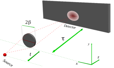
Figure 1: Sketch of the Poisson spot problem. A source of particles positioned behind of an opaque disc of radius $\beta$ send particles one-by-one and a bright spot is observed by a detector in a screen of detection. The red line along one diameter of the disc is used to illustrate the treatment of the disc as a one dimensional problem.

The propagation through the obstacle can be obtained by the Babinet principle which enables us write $\psi_{obst}(x,t,\tau)=\psi_{free}(x,t+\tau)-\psi_{slit}(x,t,\tau)$. Here, $\psi_{obst}(x,t,\tau)$ stands for the wave function describing the propagation through the obstacle, $\psi_{free}(x,t+\tau)$ the wave function for free propagation and $\psi_{slit}(x,t,\tau)$ the wave function characterizing propagation through a single slit. To calculate the corresponding wave functions, we consider that a coherent Gaussian wavepacket of initial transverse width $\sigma_{0}$ is produced at the source and propagates during a time $t$ before arriving at a single slit with Gaussian aperture from which the Gaussian wavepacket propagates. After crossing the slit the wavepacket propagates during a time $\tau$ before arriving at detector in the detection screen. The superposition of the wavepackets that propagate free and through the slit gives rise to a interference pattern as a function of the transverse coordinate $x$. Quantum effects are realized only in $x$-direction as we consider that the energy associated with the momentum of the particles in the $z$-direction is very high such that the momentum component $p_{z}$ is sharply defined, i.e., $\Delta p_{z}\ll p_{z}$. Then we can consider a classical movement in this direction with velocity $v_{z}$. Because the propagation is free, the $x$, $y$ and $z$ dimensions decouple for a given longitudinal location and thus we may write $z=v_{z}t$. Because $v_{z}$ is assumed to be a well defined velocity we can neglect statistical fluctuations in the time of flight, i.e., $\Delta t\ll t$. Such approximation leaves the Schrödinger equation analogous to the optical paraxial Helmholtz equation Viale ; Berman .

The wave functions at the screen of detection are given by

$$\psi_{free}(x,t+\tau)=\int dx_{0}K_{t}(x,t+\tau;x_{0},0)\psi_{0}(x_{0}),$$ (1)

and

$$\psi_{slit}(x,t,\tau) = \int\int dx_{j}dx_{0}K_{\tau}(x,t+\tau;x_{j},t)F(x_{j})$$ (2)

$$\times K_{t}(x_{j},t;x_{0},0)\psi_{0}(x_{0}),$$

with

$$K(x_{j},t_{j};x_{0},t_{0})=\sqrt{\frac{m}{2\pi i\hbar(t_{j}-t_{0})}}\exp\left[\frac{im(x_{j}-x_{0})^{2}}{2\hbar(t_{j}-t_{0})}\right],$$ (3)

$$F(x_{j})=\exp\left[-\frac{(x_{j})^{2}}{2\beta^{2}}\right],$$ (4)

and

$$\psi_{0}(x_{0})=\frac{1}{\sqrt{\sigma_{0}\sqrt{\pi}}}\exp\left(-\frac{x_{0}^{2}}{2\sigma_{0}^{2}}\right).$$ (5)

The kernels $K_{t}(x_{j},t;x_{0},0)$ and $K_{\tau}(x,t+\tau;x_{j},t)$ are the free propagators for the particle, the function $F(x_{j})$ describes the slit transmission function which is taken to be Gaussian of width $\beta$; $\sigma_{0}$ is the effective width of the wavepacket emitted from the source, $m$ is the mass of the particle, $t$ ($\tau$) is the time of flight from the source (slit) to the slit (screen).

After some algebraic manipulations, we obtain

$$\psi_{free}(x,t+\tau)=\frac{1}{\sqrt{b\sqrt{\pi}}}\exp\left(-\frac{x^{2}}{2b^{2}}\right)\exp\left(\frac{imx^{2}}{2\hbar r}+i\mu_{f}\right),$$ (6)

and

$$\psi_{slit}(x,t,\tau)=\frac{1}{\sqrt{B\sqrt{\pi}}}\exp\left(-\frac{x^{2}}{2B^{2}}\right)\exp\left(\frac{imx^{2}}{2\hbar R}+i\mu_{s}\right),$$ (7)

where

$$b(t+\tau)=\sigma_{0}\left[1+\left(\frac{t+\tau}{\tau_{0}}\right)^{2}\right]^{\frac{1}{2}},$$ (8)

$$r(t+\tau)=(t+\tau)\left[1+\left(\frac{\tau_{0}}{t+\tau}\right)^{2}\right],$$ (9)

$$\mu_{f}(t+\tau)=-\frac{1}{2}\arctan\left(\frac{t+\tau}{\tau_{0}}\right),$$ (10)

$$B(t,\tau)=\sqrt{\frac{\left(\frac{1}{\beta^{2}}+\frac{1}{b(t)^{2}}\right)^{2}+\frac{m^{2}}{\hbar^{2}}\left(\frac{1}{\tau}+\frac{1}{r(t)}\right)^{2}}{\left(\frac{m}{\hbar\tau}\right)^{2}\left(\frac{1}{\beta^{2}}+\frac{1}{b(t)^{2}}\right)},}$$ (11)

$$R(t,\tau)=\tau\frac{\left(\frac{1}{\beta^{2}}+\frac{1}{b(t)^{2}}\right)^{2}+\frac{m^{2}}{\hbar^{2}}\left(\frac{1}{\tau}+\frac{1}{r(t)}\right)^{2}}{\left(\frac{1}{\beta^{2}}+\frac{1}{b(t)^{2}}\right)^{2}+\frac{t}{\sigma_{0}^{2}b(t)^{2}}\left(\frac{1}{\tau}+\frac{1}{r(t)}\right)},$$ (12)

$$\mu_{s}(t,\tau)=-\frac{1}{2}\arctan\left[\frac{t+\tau\left(1+\frac{\sigma_{0}^{2}}{\beta^{2}}\right)}{\tau_{0}\left(1-\frac{t\tau\sigma_{0}^{2}}{\tau_{0}^{2}\beta^{2}}\right)}\right],$$ (13)

and

$$\tau_{0}=\frac{m\sigma_{0}^{2}}{\hbar}.$$ (14)

Here, $b(t+\tau)$, $r(t+\tau)$ and $\mu_{f}(t+\tau)$ are respectively the beam width, the radius of curvature of the wavefronts and Gouy phase for the free propagation during the total time $t+\tau$. Moreover, $B(t,\tau)$, $R(t,\tau)$ and $\mu_{s}(t,\tau)$ are respectively the beam width, the radius of curvature of the wavefronts and Gouy phase for the propagation through a single slit. $B(t,\tau)$ and $R(t,\tau)$ can be written in terms of $b(t)$ and $r(t)$, i.e, the beam width and the radius of curvature of the wavefronts for the free evolution from the source to the slit (or disc). The parameter $\tau_{0}=m\sigma_{0}^{2}/\hbar$ is viewed as a characteristic time for the “aging” of the initial state solano .

According to the Babinet principle the intensity at the screen of detection is given by

$$I(x,t,\tau) = |\psi_{obst}(x,t,\tau)|^{2}$$ (15)

$$= \frac{1}{\sqrt{\pi}b}\exp\left(-\frac{x^{2}}{b^{2}}\right)+\frac{1}{\sqrt{\pi}B}\exp\left(-\frac{x^{2}}{B^{2}}\right)$$

$$- \frac{2}{\sqrt{\pi bB}}\exp\left[-\left(\frac{1}{2b^{2}}+\frac{1}{2B^{2}}\right)x^{2}\right]$$

$$\times \cos\left[\frac{mx^{2}}{2\hbar}\left(\frac{1}{R}-\frac{1}{r}\right)+\mu(t,\tau)\right],$$

where

$$\mu(t,\tau) = \mu_{s}(t,\tau)-\mu_{f}(t+\tau)$$ (16)

$$= -\frac{1}{2}\arctan\bigg{\{}\frac{\tau[\tau_{0}^{2}+t(t+\tau)]}{\tau_{0}\tau^{2}+\frac{\beta^{2}}{\sigma_{0}^{2}}\tau[(t+\tau)^{2}+\tau_{0}^{2}]}\bigg{\}}$$

is the coherent Gouy phase difference. Therefore, from equation (15) we clearly observe the Gouy phase effect on the Poisson’s spot intensity. We illustrate such an effect in Fig. 2 by plotting the normalized intensity $I$ for the parameters of deuterium molecules of Ref. Thomas1 , i.e., $m=3.34\times 10^{-27}\;\mathrm{kg}$, $\sigma_{0}=50\;\mathrm{\mu m}$ and $\beta=60\;\mathrm{\mu m}$. We consider the propagation times $t=20\;\mathrm{ms}$ and $\tau=40\;\mathrm{ms}$. For solid line we consider and for pointed line we do not consider the Gouy phase effect. A pronounced peak at $x=0$ appears for the case in which we consider the Gouy phase difference.

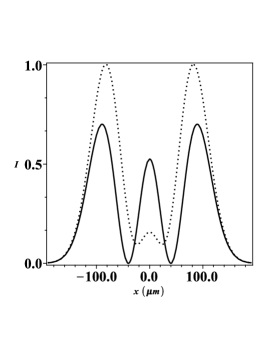
Figure 2: Gouy phase effect on the Poisson spot for a coherent model. Solid line we consider and for pointed line we do not consider the Gouy phase effect on the normalized intensity $I$.

The dependence of the Poisson’s spot intensity on the Gouy phase obviously appears corroborates the wave nature of the Poisson’s spot since the Gouy phase is a wave property. The simple model treated so far in this section does not take into account some effects that a realist model to Poisson spot have to present. It would be interesting to investigate if a more realistic model for the Poisson spot can still be related to the Gouy phase. It is the purpose of the next section to investigate such extension.

III A model with loss of coherence

The result obtained in equation (15) for the Poisson’s spot intensity does not take account any loss of coherence. We shall consider that the loss of coherence is produced from the obstacle to the screen and therefore starting from time $t+\epsilon$ (with $\epsilon\rightarrow 0$ being the propagation time through the obstacle) until the detection screen. Now, the evolution during the time $\tau$ is given by the propagator for a quantum particle interacting with an environment. In order to include such a loss of coherence we follow the result obtained in Ref. Viale and write the Poisson spot intensity as

$$I_{\ell}(x,t,\tau) \equiv \rho(x=x^{\prime},t,\tau)=N\int\int dx_{0}dx_{0}^{\prime}$$ (17)

$$\times \exp\left\{\frac{im}{2\hbar\tau}[x_{0}^{2}-x_{0}^{\prime 2}+2x(x_{0}-x_{0}^{\prime})]\right\}$$

$$\times \exp\left[-\frac{(x_{0}-x_{0}^{\prime})^{2}}{2\ell^{2}(\tau)}\right]\tilde{\rho}(x_{0},x_{0}^{\prime},t),$$

where

$$\tilde{\rho}(x_{0},x_{0}^{\prime},t)=\psi_{obst}(x_{0},t,\epsilon\rightarrow 0)\psi_{obst}^{*}(x_{0}^{\prime},t,\epsilon\rightarrow 0),$$ (18)

and

$$\ell(\tau)\equiv\frac{\ell_{0}}{\sqrt{1+\frac{2\Lambda\tau}{3}}\ell_{0}^{2}}.$$ (19)

Here, $N$ is a normalization constant, $\tilde{\rho}(x_{0},x_{0}^{\prime},t)$ is the density matrix in the obstacle, $\tau$ is the propagation time from the obstacle to the screen in which we have loss of coherence, $\ell(\tau)$ is the time dependent coherence length and $\ell_{0}$ is the coherence length in the obstacle which is the same of the source since we consider that the propagation from the source to the obstacle is free, i.e., $\ell_{0}=\ell(t)$. The parameter $\Lambda$ encodes decohering events such as scattering and photon emission and $\ell_{0}$ carries incoherence effects of the source Viale .

In order to obtain the density matrix in the obstacle we have to take the limit when $\epsilon\rightarrow 0$ in the parameters $B(t,\epsilon)$, $R(t,\epsilon)$ and $\mu_{s}(t,\epsilon)$ of the wavefunction given by equation (7). After performing such limits using the expressions (11), (12) and (13), we obtain the following results $\lim_{\epsilon\rightarrow 0}\;B(t,\epsilon)=\sqrt{\frac{b^{2}(t)\beta^{2}}{\beta^{2}+b^{2}(t)}}$, $\lim_{\epsilon\rightarrow 0}\;R(t,\epsilon)=r(t)$ and $\lim_{\epsilon\rightarrow 0}\;\mu_{s}(t,\epsilon)=\mu_{f}(t)$. Notice that only the parameter $B(t,\epsilon\rightarrow 0)$ is changed by the slit. Using the results above we obtain the density matrix in the obstacle $\tilde{\rho}(x_{0},x_{0}^{\prime},t)$.

After performing the integration in equation (17) and some algebraic manipulation we obtain

$$I_{\ell}(x,t,\tau) = \sqrt{\frac{\pi}{\eta}}\exp\left[-\frac{m^{2}x^{2}}{4\eta\hbar^{2}\tau^{2}}\right]$$ (20)

$$+ \sqrt{\frac{\pi}{\eta^{\prime}}}\exp\left[-\frac{m^{2}x^{2}}{4\eta^{\prime}\hbar^{2}\tau^{2}}\right]$$

$$- \frac{2\sqrt{2\pi\hbar\tau}}{\sqrt{\sqrt{C[1+(b(t)/\beta)^{2}]}}}\exp(-\alpha x^{2})$$

$$\times \cos(\delta x^{2}+\mu_{\ell}),$$

where

$$\eta(t,\tau) = b^{2}(t)\bigg{[}\frac{1}{2b^{2}(t)}\left(\frac{1}{2b^{2}(t)}+\frac{1}{\ell^{2}}\right)$$ (21)

$$+ \left(\frac{m}{2\hbar r(t)}+\frac{m}{2\hbar\tau}\right)^{2}\bigg{]},$$

$$\eta^{\prime}(t,\tau) = \left(\frac{\beta^{2}b^{2}(t)}{\beta^{2}+b^{2}(t)}\right)\bigg{[}\left(\frac{m}{2\hbar r(t)}+\frac{m}{2\hbar\tau}\right)^{2}$$ (22)

$$+ \left(\frac{1}{2b^{2}(t)}+\frac{1}{2\beta^{2}}\right)$$

$$\times \left(\frac{1}{2b^{2}(t)}+\frac{1}{2\beta^{2}}+\frac{1}{\ell^{2}}\right)\bigg{]},$$

$$\alpha(t,\tau) = \frac{m^{2}}{C}\left(\frac{1}{b^{2}(t)}+\frac{1}{2\beta^{2}}\right)$$ (23)

$$\times \bigg{[}\left(\frac{\beta^{2}+b^{2}(t)}{4\beta^{2}b^{2}(t)}\right)\left(\frac{1}{b^{2}(t)}+\frac{1}{\ell^{2}}\right)$$

$$+ \frac{1}{4\ell^{2}b^{2}(t)}+\left(\frac{m}{2\hbar r(t)}+\frac{m}{2\hbar\tau}\right)^{2}\bigg{]},$$

$$\delta(t,\tau)=\frac{m^{3}}{4\hbar\beta^{2}C}\left(\frac{1}{b^{2}(t)}+\frac{1}{2\beta^{2}}\right)\left(\frac{1}{r(t)}+\frac{1}{\tau}\right),$$ (24)

and

$$C(t,\tau) = 4\hbar^{2}\tau^{2}\bigg{\{}\frac{m^{2}}{16\hbar^{2}\beta^{4}}\left(\frac{1}{r(t)}+\frac{1}{\tau}\right)^{2}$$ (25)

$$+ \bigg{[}\left(\frac{\beta^{2}+b^{2}(t)}{4\beta^{2}b^{2}(t)}\right)\left(\frac{1}{b^{2}(t)}+\frac{1}{\ell^{2}}\right)$$

$$+ \frac{1}{4\ell^{2}b^{2}(t)}+\left(\frac{m}{2\hbar r(t)}+\frac{m}{2\hbar\tau}\right)^{2}\bigg{]}^{2}\bigg{\}}.$$

The Poisson spot intensity given by equation (20) is the main result of this paper. To our knowledge, an analytical expression incorporating such effects for the Poisson’s spot has not been obtained. The result of equation (20) is useful to define the Gouy phase for partially coherent matter waves and explore the role of this phase in the Poisson spot.

III.1 Generalized Gouy phase for partially coherent matter waves

In Ref. Paz1 was shown that the matter waves Gouy phase is related with the off diagonal elements of the covariance matrix which indirectly enabled to extract the Gouy phase from the beam width. It was shown that the experimental data for the diffraction of fullerene molecules is quantitatively consistent with the existence of a Gouy phase. Since the fullerene molecules have to be treated as partially coherent matter waves in that work was conjectured that the Gouy phase can be obtained by integrating the inverse of the squared beam width, as is valid for coherent case. Further, a complete definition for the Gouy phase for partially coherent light waves was given in Ref. Visser . In this work we use the definition of Ref. Visser to obtain the Gouy phase for partially coherent matter waves as

$$\mu_{\ell}(t,\tau)=\arg[I_{\ell}(0,t,\tau)].$$ (26)

We have a complete analogy with the generalized definition for the Gouy phase of Ref. Visser , since here $I_{\ell}(0,t,\tau)\equiv\rho(0,t,\tau)$ is the density matrix in the propagation axis $z$ which is similar to the cross-spectral density and $(t,\tau)$ can be used to obtain two different positions in the propagation axis since we are substituting the propagation time by $z/v_{z}$. In the case of light waves the mechanism of loss of coherence is attributed to the source incoherence whereas for matter waves such effects can be attributed both to the source incoherence and environment decoherence. We calculate the Gouy phase here and obtain the following result

$$\mu_{\ell}(t,\tau)=-\frac{1}{2}\arctan\left[\frac{r(t)+\tau}{a_{1}+a_{2}+\frac{r(t)\tau}{\tau_{0}}\left(1+\frac{2\beta^{2}}{b^{2}(t)}\right)\frac{\sigma_{0}^{2}}{\ell^{2}}}\right],$$ (27)

where

$$a_{1}(t,\tau)=\left(\frac{\beta^{2}\tau_{0}}{\sigma_{0}^{2}r(t)\tau}\right)(r(t)+\tau)^{2},$$ (28)

and

$$a_{2}(t,\tau)=\frac{r(t)\tau}{\tau_{0}}\left(1+\frac{\beta^{2}}{b^{2}(t)}\right)\left(\frac{\sigma_{0}}{b(t)}\right)^{2}.$$ (29)

We can observe from equation (27) that the Gouy phase is dependent of the coherence length $\ell$. The same dependence was discussed in Ref. Visser for partially coherent light wave. We can easily obtain that the result of equation (27) reduces to that of equation (16) for coherent matter waves in the limit $\ell\rightarrow\infty$. On the other hand, in the limit of completely non-coherent matter waves $\ell\rightarrow 0$ we have $\mu_{\ell}\rightarrow 0$.

Therefore, just as in the coherent case the Poisson spot intensity is changed by the Gouy phase. This can be clearly seen in the figure below. In Fig. 3(a) we show the Gouy phase $\mu_{\ell}(t,\tau)$ as a function of the propagation time $\tau$ for $t=20\;\mathrm{ms}$ and for the data of the deuterium molecules. Solid line corresponds to $\ell=1.0\;\mathrm{m}$ and pointed line corresponds to $\ell=100\;\mathrm{\mu m}$. In Fig. 3(b) we show the normalized intensity $I_{\ell}$ as a function of $x$ for $t=20\;\mathrm{ms}$ and $\tau=40\;\mathrm{ms}$ for the data of deuterium molecules. Solid line we consider the effect of the phase $\mu_{\ell}$ and pointed line we do not consider such effect.

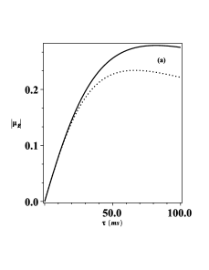
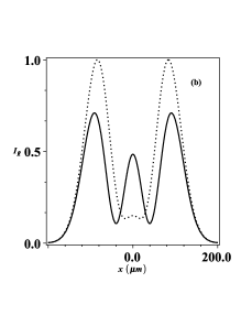
Figure 3: (a) Gouy for partially coherent matter waves as a function of $\tau$ for two different values of coherence length and $t=20\;\mathrm{ms}$. Solid line corresponds to $\ell=1.0\;\mathrm{m}$ and pointed line corresponds to $\ell=100\;\mathrm{\mu m}$. (b) Normalized intensity $I_{\ell}$ as a function of $x$ for $\ell=100\;\mathrm{\mu m}$, $t=20\;\mathrm{ms}$ and $\tau=40\;\mathrm{ms}$. Solid line we consider the effect of the phase $\mu_{\ell}$ and pointed line we do not consider such effect.

Fixing a set values of parameters we observe that the Gouy phase decreases when the coherence length decreases. This is a novel result in the context of matter waves. The visibility of the Poisson spot tends to decrease as an effect of the loss of coherence. We can observe this by comparing the intensity for the coherent and partially coherent case, Fig. 2 and Fig. 3(b) respectively, which show that the minimum intensity for the partially coherent case is not zero. The partially coherent Gouy phase changes the intensity in a such way that the intensity in the central peak is not observed if one neglected this phase. The presence of the Gouy phase is a signature of the wave behaviour. Thus, the relationship between Poisson spot and Gouy phase for a model of partially coherent matter waves with analytical results as obtained in this section is useful to treat experimental data and to elucidate the wave behaviour of the Poisson spot with matter waves. In order to test our results in the next section we will analyse the experimental data for deuterium molecules of Ref. Thomas1 .

IV Analysis of existing experimental data

In this section we compare our model with the experimental data for deuterium molecules of Ref. Thomas1 . We take into account loss of coherence and the finite detection area. The loss of coherence was obtained in equation (20). To include the detector effect we perform a convolution to obtain the effective intensity

$$I_{eff}(x,t,\tau)=\int^{\infty}_{-\infty}I_{\ell}(x^{\prime},t,\tau)D(x-x^{\prime})dx^{\prime}.$$ (30)

Considering a Gaussian profile to the detector aperture as $D(x)=\exp\left(-x^{2}/2\sigma_{D}^{2}\right)$, where $\sigma_{D}$ is the detector width, the integral above is easily done.

In order to compare our model with experimental results previously published in Ref. Thomas1 we relate our model and the one in Thomas1 by $I_{eff}(x,l,\sigma_{D})=a+b\;I(x,l,\sigma_{D})$. The parameters $a$ and $b$ are necessary to convert our results in units ($rate/s$) used in Ref. Thomas1 . The numerical calculations obtained within these units are summarized in Table 1. The obtained results are in good agreement with the experimental values, as we can observe in Fig. 4.

Table 1: Parameters of analytic model and numerical results

Coherence parameter	$\ell=0.3369\;\mathrm{\mu m}$
Detector width	$\sigma_{D}=3.96\;\mathrm{\mu m}$
Gaussian width	$\sigma_{0}=51\;\mathrm{\mu m}$
Disc aperture	$\beta=60\;\mathrm{\mu m}$
Time before disc	$t=1.4\;\mathrm{ms}$
Time after disc	$\tau=0.606\;\mathrm{ms}$
Partially coherent fit [PC] b	$a=29829.11,\;b=-348.71$
Detector convolution fit [DC]	$a=40465.09,\;b=-466.29$
Gouy Phase [PC]	$\mu_{\ell}=0.00060097028\;\mathrm{rad}$
Gouy Phase [DC]	$\mu_{\ell}=0.00069360626\;\mathrm{rad}$

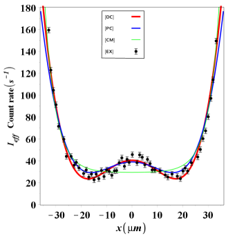
Figure 4: Comparison of experimental data Ref. Thomas1 with analytical model (table 1). Black points with error bars are the experimental data. Green line is the coherent model. Blue line is the model with loss of coherence and red line is the model with loss of coherence and detector convolution.

We observe by red line of Fig. 4 that an analytical model including loss of coherence as well as finite detector area is in full agreement with existing experimental data. On the other hand, the blue line shows that considering only loss of coherence there is an agreement between the model and the experimental data but to obtain a full agreement it is necessary to consider the detector convolution. Green line shows that is not possible to adjust the data by considering a completely coherent model. In the adjustment a given value of partially coherent Gouy phase is necessary. The small value found here is related with the set value of parameters used in the experiment, specially the propagation times. Therefore, different values of partially coherent Gouy phase can be obtained if the experiment is realized with different set value of parameters.

V Conclusions

We developed a theoretical model for the Poisson’s spot problem by using the Babinet principle. It was possible to include loss of coherence and detector convolution in the observed intensity. Firstly, we treated the coherent model and then we studied the effect of the loss of coherence. Based in the previous definition to the Gouy phase for partially coherent light waves (source incoherence) we obtained an expression to the Gouy phase for partially coherent matter waves (source incoherence + environment decoherence). We observed that this phase influences the Poisson spot intensity. Therefore, we have found a relationship between two old physical problems (Gouy phase and Poisson spot). We obtained full agreement between our results and existent experimental data. We observed that the Gouy phase depends on the set value of parameters used in the Poisson spot experiment. Thus, the Poisson spot experiment can be used to measure the Gouy phase for partially coherent matter waves.

- (1) A. J. Fresnel, OEuvres Completes I (Imprimerie imperiale, Paris, 1868); J. E. Harvey and J. L. Forgham, Am. J. Phys., 52, 243 (1984); E. Hecht, Optics, 4th international ed. (Addison Wesley, Boston, 2002); D. Gooding, T. Pinch, and S. Schaffer, The Uses of Experiment: Studies in the Natural Sciences (Cambridge University Press, Cambridge, UK, 1989).
- (2) M. Arndt, O. Nairz, J. Vos-Andreae, C. Keller, G. van der Zouw, and A. Zeilinger, Lett. to Nat. 401, 680 (1999).
- (3) J. Komrska, Advances in Electronics and Electron Physics (Academic, New York, 1971), pp. 139-234; G. Matteucci, Am. J. Phys. 58, 1143 (1990).
- (4) T. Reisinger et al, Phys. Rev. A 79, 053823 (2009).
- (5) T. Reisinger, G. Bracco, and B. Holst, New Journal of Phys. 13, 065016 (2011).
- (6) T. Juffmann, S. Nimmrichter, M. Arndt, H. Gleiter, and K. Kornberger, Found. of Phys. 42, 075002 (2011).
- (7) J. L. Hemmerich, R. Bennett, T. Reisinger, S. Nimmrichter, J. Fiedler, H. Hahn, H. Gleiter, and S. Y. Buhmann, Phys. Rev. A 94, 023621 (2016).
- (8) Y. Zhang, W. Zhang, M. Su, and L. Chen, Journal of the Optical Society of America A 33, 570 (2016).
- (9) L. G. Gouy, C. R. Acad. Sci. Paris 110, 1251 (1890).
- (10) L. G. Gouy, Ann. Chim. Phys. Ser. 6 24, 145 (1891).
- (11) T. D. Visser and E. Wolf, Opt. Comm. 283, 3371 (2010).
- (12) R. Simon and N. Mukunda, Phys. Rev. Lett. 70, 880 (1993).
- (13) S. Feng and H. G. Winful, Opt. Lett. 26, 485 (2001).
- (14) J. Yang and H. G. Winful, Opt. Lett. 31, 104 (2006).
- (15) R. W. Boyd, J. Opt. Soc. Am. 70, 877 (1980).
- (16) P. Hariharan and P. A. Robinson, J. Mod. Opt. 43, 219 (1996).
- (17) S. Feng, H. G. Winful, and R. W. Hellwarth, Opt. Lett. 23, 385 (1998).
- (18) X. Pang, T. D. Visser, and E. Wolf, Opt. Comm. 284, 5517 (2011); X. Pang, G. Gbur, and T. D. Visser, Opt. Lett. 36, 2492 (2011); X. Pang and T. D. Visser, Opt. Exp. 21, 8331 (2013); X. Pang, D. G. Fischer, and T. D. Visser, Opt. Lett. 39, 88 (2014).
- (19) C. J. S. Ferreira, L. S. Marinho, T. B. Brasil, L. A. Cabral, J. G. G. de Oliveira Jr, M. D. R. Sampaio, and I. G. da Paz, Ann. of Phys. 362, 473 (2015).
- (20) D. Chauvat, O. Emile, M. Brunel, and A. Le Floch, Am. J. Phys. 71, 1196 (2003).
- (21) N. C. R. Holme, B. C. Daly, M. T. Myaing, and T. B. Norris, Appl. Phys. Lett. 83, 392 (2003).
- (22) W. Zhu, A. Agrawal, and A. Nahata, Opt. Exp. 15, 9995 (2007).
- (23) T. Feurer, N. S. Stoyanov, D. W. Ward, and K. A. Nelson, Phys. Rev. Lett. 88, 257 (2002).
- (24) A. Hansen, J. T. Schultz, and N. P. Bigelow, Conference on Coherence and Quantum Optics Rochester (New York, United States, 2013); J. T. Schultz, A. Hansen, and N. P. Bigelow, Opt. Lett. 39, 4271 (2014).
- (25) G. Guzzinati, P. Schattschneider, K. Y. Bliokh, F. Nori, and J. Verbeeck, Phys. Rev. Lett. 110, 093601 (2013); P. Schattschneider, T. Schachinger, M. Stöger-Pollach, S. Löffler, A. Steiger-Thirsfeld, K. Y. Bliokh, and F. Nori, Nature Communications 5, 4586 (2014).
- (26) T. C. Petersen, D. M. Paganin, M. Weyland, T. P. Simula, S. A. Eastwood, and M. J. Morgan, Phys. Rev. A 88, 043803 (2013).
- (27) A. E. Siegman, Lasers, University Science Books, Sausalito CA, 1986.
- (28) Ph. Balcou and A. L. Huillier, Phys. Rev. A 47, 1447 (1993); M. Lewenstein, P. Salieres, and A. L. Huillier, Phys. Rev. A 52, 4747 (1995); F. Lindner, W. Stremme, M. G. Schatzel, F. Grasbon, G. G. Paulus, H. Walther, R. Hartmann, and L. Struder, Phys. Rev. A 68, 013814 (2003).
- (29) F. Lindner, G. Paulus, H. Walther, A. Baltuska, E. Goulielmakis, M. Lezius, and F. Krausz, Phys. Rev. Lett. 92, 113001 (2004).
- (30) L. Allen, M. W. Beijersbergen, R.J.C. Spreeuw, and J.P. Woerdman, Phys. Rev. A 45, 8185 (1992); L. Allen, M. Padgett, and M. Babiker, Prog. Opt. 39, 291 (1999).
- (31) I. G. da Paz, M. C. Nemes, S. Pádua, C. H. Monken, and J. J. Peixoto de Faria, Phys. Lett. A 374, 1660 (2010).
- (32) I. G. da Paz, P. L. Saldanha, M. C. Nemes, and J. G. Peixoto de Faria, New Journal of Phys. 13, 125005 (2011).
- (33) R. Ducharme and I. G. da Paz, Phys. Rev. A 92, 023853 (2015).
- (34) I. G. da Paz, C. H. S. Vieira, R. Ducharme, L. A. Cabral, H. Alexander, and M. D. R. Sampaio, Phys. Rev. A 93, 033621 (2016).
- (35) M. Born and M. Wolf, Principles of Optics, Cambridge University Press, Cambridge, 1999.
- (36) A. Viale, M. Vicari, and N. Zanghi, Phys. Rev. A 68, 063610 (2003).
- (37) X. Pang, D. G. Fischer, and T. D. Visser, J. Opt. Soc. Am. A 29, 989 (2012).
- (38) P. R. Berman, Atom Interferometry, San Diego, Academic Press, 1997, pp 175.
- (39) J. S. M. Neto, L. A. Cabral, and I. G. da Paz, Eur. J. Phys. 36, 035002 (2015).