Probing the Active Galactic Nuclei Unified Model Torus Properties in Seyfert Galaxies

Abstract

We studied the physical parameters of a sample comprising of all Spitzer/IRS public spectra of Seyfert galaxies in the mid-infrared (5.2-38 $\mu$m range) under the active galactic nuclei (AGN) unified model. We compare the observed spectra with $\sim 10^{6}$ clumpy model spectral energy distributions, which consider a torus composed of dusty clouds. We find a slight difference in the distribution of line-of-sight inclination angle, $i$, requiring larger angles for Seyfert 2 (Sy 2) and a broader distribution for Seyfert 1 (Sy 1). We found small differences in the torus angular width, $\sigma$, indicating that Sy 1 may host a slightly narrower torus than Sy 2. The torus thickness, together with the bolometric luminosities derived, suggest a very compact torus up to $\sim$6 pc from the central AGN. The number of clouds along the equatorial plane, $N$, as well the index of the radial profile, $q$, are nearly the same for both types. These results imply that the torus cloud distribution is nearly the same for type 1 and type 2 objects. The torus mass is almost the same for both types of activity, with values in the range of $M_{tor}\sim$10${}^{4}-$10${}^{7}\rm M_{\odot}$. The main difference appears to be related to the clouds’ intrinsic properties: type 2 sources present higher optical depths $\tau_{V}$. The results presented here reinforce the suggestion that the classification of a galaxy may depend also on the intrinsic properties of the torus clouds rather than simply on their inclination. This is in contradiction with the simple geometric idea of the unification model.

1 Introduction

According to the unified model, the energy from active galactic nuclei (AGN) is powered by the accretion of matter into a supermassive black hole (SMBH) (Lynden-Bell, 1969; Begelman et al., 1984). The unification scheme suggests that the different AGN types are explained by the line-of-sight (LOS) orientation of an obscuring material, which surrounds the central source and is arranged in an axisymmetric/toroidal geometry and composed primarily of gas and dust. Under edge-on views, it obscures the radiation from the accretion disk and broad line region (BLR). Such an object is classified as a type 2 AGN. When viewed face-on, the central engine can be observed directly. These galaxies are classified as type 1 AGNs (Antonucci, 1993; Urry & Padovani, 1995). The unified model was firstly supported through spectropolarimetric observations of the Seyfert 2 (Sy 2) galaxy NGC 1068 (Antonucci & Miller, 1985), revealing the polarized broad emission lines, and followed by other polarized broad line observations in type 2 AGNs (e.g., by Tran et al., 1992; Tran, 1995). This hidden type 1 emission can be visible via light scattering in the ionizing cones, which corresponds to ionizing radiation that is collimated by the torus opening angle, providing additional indirect evidence for the unified model (e.g., Pogge, 1988; Storchi-Bergmann & Bonatto, 1991; Storchi-Bergmann et al., 1992).

The dusty structure of the AGN unified model is responsible for absorbing short wavelength light from the active nucleus and re-emitting it mainly in the infrared (IR) wavelengths, leading to a peculiar signature in the spectral energy distribution (SED) of a galaxy. In specific, the silicate feature at 9.7 $\mu$m in the mid-infrared (MIR) is frequently found in absorption in type 2 and is also expected to appear in emission in type 1. However, in most type 1 objects this feature is either mild or absent (Hao et al., 2007; Wu et al., 2009). In addition, there are some cases where silicate emission is detected in type 2 (e.g., in Sy 2 NGC 2110 by Mason et al., 2009; Sturm et al., 2006). Consequently, the MIR spectral range hosts fundamental features necessary to study the putative torus required in the Unified Model for AGNs. The recent significant advances in observational facilities, such as ALMA and VLTI, now allow us to resolve the central parsec scales in nearby AGNs. So far, only a few VLBI observations achieve sufficient spatial resolution to isolate the emission of these obscured structures. For instance, the cases of NGC 1068 (Gratadour et al., 2015; Jaffe et al., 2004; López-Gonzaga et al., 2014) and Circinus (Tristram et al., 2007, 2014). Very recently, García-Burillo et al. (2016) and Imanishi et al. (2016) presented the first resolved images of the torus of NGC 1068, the former using the continuum and the CO(6-5) emission observed with ALMA Band 9 and the latter using HCN(3-2) and HCO⁺(3-2) emission lines. These cases are successful precedents for forthcoming ALMA observations intended to study molecular gas in the torus and its surrounding (Netzer et al., 2015). While there are no plenty of data with such detailed observations, the optimal way to probe the physical processes related to the torus is understanding the radiation reprocessing mechanisms responsible for the singular behaviour of the AGN SEDs.

In the last two decades, several models have been developed in order to understand the torus emission. For example, Krolik & Begelman (1988) proposed that the torus should constitute of a large number of optically thick dusty clouds, otherwise the dust grains would be destroyed by the high AGN energy luminosity. Their presumption is reinforced by VLTI interferometric observations in the N-band range (8–13 $\mu$m) performed by Tristram et al. (2007) in the nucleus of the Circinus galaxy, providing strong evidence of a clumpy and dusty structure. Due to computational issues in modelling a clumpy medium, some studies have explored the effect of a dusty uniform distribution in a toroidal geometry (Pier & Krolik, 1992; Granato & Danese, 1994; Efstathiou & Rowan-Robinson, 1995; Dullemond & van Bemmel, 2005; Fritz et al., 2006). However, to explain the low resolution ($>$1”) observed SEDs and IR spectra in such homogeneous descriptions, the models force the torus size to be at scales of $\gtrsim$100 pc. With the advent of high-spatial resolution using 8$m$-class telescopes, it was demonstrated that the surrounded dusty environment is much more compact, with sizes of a few parsecs (Jaffe et al., 2004; Tristram et al., 2009; Burtscher et al., 2009).

Nevertheless, in the last few years, some efforts have been made to handle a clumpy formalism and they can naturally explain the problem with the silicate issue mentioned above (Nenkova et al., 2002; Hönig et al., 2006; Nenkova et al., 2008a, b; Schartmann et al., 2008; Stalevski et al., 2012). Among them, the clumpy models presented by Nenkova et al. (2002, 2008a, 2008b) are, to date, some of the most successful models for representing the re-processed MIR torus emission and allowing us to constrain some torus properties. They consist of a large database of theoretical SEDs resulting from a 1D radiative transfer code (dusty, Ivezic et al., 1999) taking into account the continuum emission from clumpy media with shadowed individual clouds. One of the advantages of a clumpiness formalism is that they can reproduce more realistic MIR spectra. This is because they have a wide range of dusty cloud temperatures at the same radius from the central source and even distant clouds can be directly illuminated by the AGN, contrary to the smooth density distributions. The clumpy models have been used by several works to study the torus properties, for example, in a sample of 26 quasar by Mor, Netzer & Elitzur (2009), in a analysis of 27 Sy 2 by Lira et al. (2013) and in modest to small samples of Seyfert galaxies (e.g. Ichikawa et al., 2015) and the works from Alonso-Herrero et al. (2011); Ramos Almeida et al. (2009, 2011), hereafter, AH11, RA09 and RA11, respectively. One of the main differences between our work and AH11 and RA11 is the use of near infrared (NIR) data for all the galaxies in their analysis and our much larger sample.

We investigated the torus properties of 111 Seyfert galaxies using data archive from Infrared Spectrograph (IRS, Houck et al., 2004) aboard the Spitzer Space Telescope in the 5.2–38 $\mu$m spectral range. We compared the sample with the clumpy theoretical SEDs from Nenkova et al. (2002, 2008a, 2008b) using two different approaches: the $\chi_{red}^{2}$ test as well as bayesian inference (BayesClumpy, Asensio Ramos & Ramos Almeida, 2009). Section 2 characterizes the sample and data reduction. In section 3 we describe the clumpy models, the PAH’s decontamination from the SEDs and the different approaches utilized to fit the data. Main results and the discussion are summarized in Section 4 and the contribution of the NIR data is exploited in Section 5. Our conclusions are presented in Section 6.

2 The Data

We have performed an analysis on a sample of 111 nearby galaxies classified as Seyfert galaxies that were available in the Spitzer Heritage Archive. The sample consists of 84 galaxies that have been presented in previous works (Gallimore et al., 2010; Wu et al., 2009), 14 galaxies from Sales et al. (2010) and another 13 objects available in the Spitzer archive (presented here for the first time). The galaxies were observed with the IRS using two low spectral resolution (R$\sim$60-127) modules: Short-Low (SL) and Long-Low (LL), covering a wavelength range from 5.2 to 38 $\mu$m in the MIR. The SL module has an image scale of 1.8”/pixel and the LL module 5.1”/pixel. Both are sub-divided in order 1 and 2.

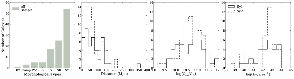
Figure 1: Characteristics of the 111 AGN samples. The solid line histograms show the properties for Seyfert 1 galaxies while the dashed lines represent the Seyfert 2 sources. Morphological classification and distances were obtained from the NED - NASA/IPAC Extragalactic Database or from Whittle (1992). In the left panel, we gathered all morphological types into 7 mean classes: irregular (Irr), compact (Comp), peculiar (Pec), elliptical (E), spiral (S), lenticular (S0) and barred spiral (SB). The references for L_IR and L_X can be founded in Table LABEL:obs:tab1.

With the exception of 7 galaxies whose spectra are available from the SINGS Legacy program (PID 159, Kennicutt et al., 2003), all other data were processed using the Basic Calibration Data (BCD) pipeline (version 18.18). The BCD pipeline manages the raw data through basic processing, such as the detection of cosmic rays, the removal of saturated pixels, dark current and flat-field subtraction and droop correction. For the sample presented in Gallimore et al. (2010), 78 objects have the spectral mapping mode available, while the other 6 present the mapping mode only in LL and SL observations in the staring mode (NGC 526A, NGC 4941, NGC 3227, IC 5063, NGC 7172 and NGC 7314).

The mapping mode observations were processed by employing the CUbe Builder for IRS Spectra Maps (CUBISM, Smith et al., 2007a) to construct the data cubes. Sky subtraction were evaluated from an average spectra of the off-source orders: e.g. while the source is centred in the first order, the second order is pointed at the sky in an offset position. We used a 3.9$\times$11.1 pixel extraction (equivalent to a 10” circular radius aperture centred on the brightest source) to extract the spectra. In a few cases the extractions showed a mismatch between the modules or their orders that was corrected by scaling the spectra as recommended by Smith et al. (2007b).

For the remaining 27 objects the data are available in staring mode and the calibrated spectra were obtained from the Cornell Atlas of Spitzer/IRS Sources (CASSIS, Lebouteiller et al., 2011). CASSIS provides optimal extractions and diagnostic tools to guarantee the most accurate background subtraction, especially for faint sources. In most cases, the optimal CASSIS extraction pointed to sky subtraction through the off-order method. However, in a few cases, CASSIS indicated the subtraction by nod positions as the best spectral extraction. Furthermore, the majority of CASSIS products were established as point-like sources.

Our final sample is composed of 45 Sy 1 and 65 Sy 2 galaxies with redshifts between 0.002 $\leq$ $z$ $\leq$ 0.079. The AGNs are preferentially found in host galaxies with barred spiral, lenticulars or in spiral morphological types. The mean values for the IR luminosities are L_IR(Sy1)= 4.64$\times$10${}^{10}\rm L_{\odot}$ for Sy 1 and L_IR(Sy2)= 5.44$\times$10${}^{10}\rm L_{\odot}$ and for the hard X-ray luminosities are L_2-10Kev(Sy1)= 1.59$\times$10⁴³ and L_2-10Kev(Sy2)= 1.19$\times$10⁴³ erg $\rm s^{-1}$. The sample properties are summarized in Figure 1 and listed in Table LABEL:obs:tab1.

2.1 Removing the PAH Contamination

Since the IRS Spitzer spectra were extracted in a 20” circular diameter aperture, corresponding to $\sim$1-20 Kpc of the galaxies (except for z=0.79, Mrk478 which represents $\sim$33 Kpc), the host galaxy contribution is unavoidable in our sample. In order to minimize the effects from star formation and to isolate the AGN emission of the galaxy, we have adopted a similar method as that used in Lira et al. (2013). They remove the stellar contribution by subtracting templates developed by Smith et al. (2007b), when the MIR is dominated by polycyclic aromatic hydrocarbons (PAHs) emission of star forming regions.

Instead of fitting star formation templates, we chose to follow another approach in order to attenuate the PAH’s contribution (and therefore, that of the host galaxy) in the spectra. We applied the pahfit tool developed by Smith et al. (2007b). This code decomposes the emission lines of the low resolution IRS Spitzer spectra, modelling them as the sum of starlight continuum, thermal dust continuum, and emission lines (pure rotational lines of H₂, fine structure lines, and dust emission features). All flux intensity components are affected by dust extinction, quantified by the optical depth (for more details, see Smith et al., 2007b).

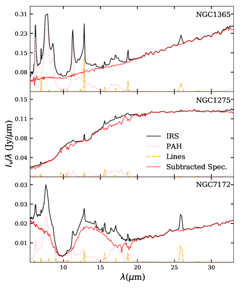
Figure 2: Typical examples of the subtraction of the PAH and ionic line components from the spectra. The black lines represent the observed spectra, while the dotted/dashed orange and dashed pink lines show the resulting adjusted spectra created by fitting the PAH emission and ionic and hydrogen lines, respectively, using the pahfit tool. In the dotted red lines are the subtracted spectra that were handled in our analysis. In the top panel the results for NGC 1365 are shown, characterizing a galaxy with strong PAH emission. On the other hand, the middle panel shows little contribution from this feature for NGC 1275. An example of a deep silicate absorption and PAH emission is presented in the bottom panel for the Sy 2 NGC 7172.

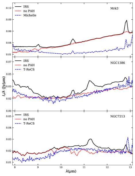
Figure 3: We show a comparison of the low resolution Spitzer IRS spectra and the ground based nuclear emission observations. The top panel shows the spectrum of Mrk 3 from Michelle while the middle and bottom panels present the data from T-ReCs for NGC 1386 and NGC 7213, respectively. The black lines represent the IRS data, the dotted red lines the starburst subtracted spectra and the dashed blue lines the high resolution spectra. Except in the case of Mrk 3, the subtracted spectra appear to well represent the emission from the active nucleus.

Since the continuum from our Seyfert sample is not only due to dust and stellar components, but also to the AGN power-law continuum, we decided to subtract only the emission lines from the H₂ and the molecular features of PAH emission from the observed spectra. It is, however, worth mentioning that most of the PAH contribution lies in 5-15 $\mu$m, where the stellar emission is more prominent. For longer wavelengths, the host galaxy emission is very difficult to distinguish from the AGN continuum, and unfortunately, the current spectral decomposition codes are unable to separate each contribution for $\lambda\gtrsim$20 $\mu$m (e.g., Smith et al., 2007b; Hernán-Caballero et al., 2015). This trend might overestimate AGN emission at longer wavelengths, which could bias the outputs of the CLUMPY models towards extended and broader tori, due to the cooler dust that peaks in the far-infrared range. Nonetheless, recently Fuller et al. (2016) separated the AGN and PAH components using the full wavelength coverage of the Spitzer/IRS spectra of 11 Seyfert galaxies. They used the templates provided by Hernán-Caballero et al. (2015) and then compared the AGN resulting spectra with the 31.5 $\mu$m imaging photometry from the Stratospheric Observatory For Infrared Astronomy (SOFIA), finding that most of the sources are AGN dominated at 31.5 $\mu$m.

In Figure 2 we present some representative examples of this approach. Shown is a case with strong PAH emission and second with little PAH feature contribution (Sy 1 NCG 1365 and Sy 2 NGC 1275 respectively). Also, we selected an example of deep silicate absorption in 9.7 $\mu$m for NGC 7172, which is surrounded by PAH emission. As can be seen, the effect of the molecular emission features is more prominent at shorter wavelengths and can alter the shape of the spectrum. The majority of galaxies (about 80% of the sample) exhibit a substantial star forming contribution (see also Sales et al., 2010).

Recently, some other studies have been supporting this star forming subtraction methodology. For instance, in Ruschel-Dutra et al. (2014) there is no PAH emission detected using high resolution nuclear spectra from T-ReCs when compared with IRS observations of NGC 7213 and NGC 1386. Also, no PAH emission bands were detected in the nuclear region ($\sim$200 pc) of Mrk 3, a Compton-thick Sy 2, using Michelle/Gemini spectrograph (Sales et al., 2014). Davies et al. (2012) argued that the PAH molecules can not survive in a radius smaller than 50 pc, a value corresponding to a region larger than that of the torus extension (parsec scale, Tran et al., 1992). However, in some cases, e.g. in T-ReCs observations of NGC1808, the aromatic component was detected at 8.6 and 11.3$\mu$m in the galaxy centre ($\sim$26 pc) up to a radius of 70 pc from the nucleus (Sales et al., 2013).

To illustrate the effect of the starburst subtraction method, we show in Figure 3 the high resolution data from Michelle and T-ReCs of the galaxies Mrk 3, NGC 1386 and NGC 7213, compared to the IRS spectra. Also shown is the final spectra resulting from the subtraction of the PAH components. The clean IRS spectra tends to better approximate the nuclear spectra from high resolution observations, except for the Mrk 3. This is possibly due to the fact that this galaxy is a Compton-thick object and has a heavy absorbed dust/gas component ($N_{H}\sim 1.1\times 10^{24}\rm cm^{-2}$, Sales et al., 2014) obscuring the nucleus, leading to a higher continuum in the Spitzer observation. Moreover, the fact of this galaxy has a small starburst contribution may explain why we see almost no differences between the IRS spectra and the subtracted one. However, in the cases of NGC 1386 and NGC 7213, we believe that the PAH subtraction approach represents a good approximation of the nuclear emission. Thus, the spectral decomposition methodology was applied to all the objects used in our study.

3 Modelling the SED in the MIR

3.1 clumpy Torus Models

A clumpy medium provides a natural explanation for the silicate absorption feature that was expected to be observed in emission in type 1 sources but is frequently mild or even flat, since it requires at least a clump obscuring the radiation at the observer’s LOS.

The most successful and up to date clumpy models are those of the Kentucky group. Nenkova et al. (2002, 2008a, 2008b) developed a formalism to handle a clumpy media, considering point-like dusty clouds distributed in a toroidal geometry around the central AGN. The clumpy models are a large database ($\sim$10⁶) of theoretical SEDs resulting from the radiative transfer treatment through the dusty code (Ivezic et al., 1999). The dust grains follow the MNR size distribution (Mathis, Rumpl & Nordsieck, 1977) and are composed by the standard Galactic mixture of 47% graphite with optical constants and 53% cold silicates. While the graphite grains are the responsible for the IR emission at $\lambda\gtrsim 1\mu$m, the 9.7 $\mu$m and 18 $\mu$m emission and absorption features are attributed to silicate grains (e.g. Barvainis, 1987; Pier & Krolik, 1992; Granato & Danese, 1994; Siebenmorgen et al., 2004).

The clumpy models assume that the torus is formed by dusty clumps constrained by the following parameters: (i) the number of clouds, $N_{0}$ , in the torus equatorial radius; (ii) $\tau_{V}$, the optical depth of each cloud defined at 0.55 $\mu$m band; (iii) the radial extension of the clumpy distribution, $Y=R_{o}/R_{d}$, where $R_{o}$ and $R_{d}$ are the outer and inner radius of the torus, respectively; (iv) the radial distribution of clouds as described by a power law $r^{-q}$; (v) the torus angular width, $\sigma$, constrained by a Gaussian angular distribution width and (vi) the observers viewing angle $i$. The grid of these model parameters are listed in Table LABEL:obs:tab2.

Table 1: Parameters values adopted in fitting

	Sampled Values	Description
clumpy Models
$i$	0-90 steps of 10∘	Observer’s viewing angle
$N$	1-15 steps of 1	Clouds along the equatorial plane
$q$	0-3 steps of 0.5	Power law index of the radial distribution
$\tau_{V}$	5,10,20,30,40,60,80,100,150	Optical depth of individual clouds
$\sigma$	15-70 steps of 5	Torus angular width
$Y$	5, 10-100 steps of 10	Torus thickness

The model geometry also allow us to determine other parameters that are crucial to understand the obscuration effects of the central source. They are the number of clouds along the LOS, $N_{los}$, described by almost a Gaussian distribution along the equatorial plane ($N$), which depends on the inclination, $\beta=\pi/2-i$, and angular width, $\sigma$, parameters

$$N_{los}(\beta)=Nexp^{-{\left(\frac{\beta}{\sigma}\right)}^{2}}$$ (1)

and the total optical depth of the torus along the LOS, product of the number of clouds and the optical depth of each cloud, or, the visual extinction:

$$A_{V}=1.086N_{los}\tau_{V}$$ (2)

One of the characteristics of Nenkova et al. models is that the SEDs reproduced are not exclusively sensitive to the inclination angle, as established by the only orientation dependent unification schemes. The continuum shape and behaviour of the silicate features also have a strong dependence with the optical properties, characterized by the optical depth $\tau_{V}$, and the number of clouds along radial rays, specifically at the equatorial plane, $N$. In the latter, $N$ must be sufficient large, $N\sim$5–10, to assure the attenuation of X-rays in type 2 sources while the former one was constrained to values $\tau_{V}\gtrsim$60 to ensure the probability of photon escape. The explanation for many problems faced by the smoothly distribution handling are answered by the clumpiness nature of the toroidal structure and, therefore, the clumpy models constitute a powerful tool to probe the torus physical properties proposed by the AGN’s Unified Model.

3.2 Fitting Procedure

Once we applied the procedure to isolate the nuclear emission, we performed two different approaches to compare the MIR resulting spectra from IRS observations with Nenkova’s theoretical models. In the following sections we describe the techniques employed.

3.2.1 $\chi^{2}_{red}$ test

We developed a code to compare each spectrum with all $10^{6}$ clumpy models SEDs. The routine searches for the parameters which minimizes the equation:

$${\chi_{red}}^{2}=\frac{1}{N}\sum_{i=1}^{N}{\left(\frac{F_{obs,\lambda_{i}}-F_{mod,\lambda_{i}}}{\sigma_{\lambda_{i}}}\right)}^{2}$$ (3)

where N is the number of data points in the spectrum, $F_{obs,\lambda_{i}}$, and $F_{mod,\lambda_{i}}$, are the observed and theoretical fluxes at each wavelength and $\sigma_{\lambda_{i}}$ are the uncertainties in $F_{obs,\lambda_{i}}$. Both $F_{obs,\lambda_{i}}$ and $F_{mod,\lambda_{i}}$ were normalized to unit at 28.0$\mu$m for all the galaxies in the sample, with the uncertainties correctly propagated. The “decontaminated” nuclear spectrum was compared to the clumpy theoretical SEDs and we test the results for the best fit, e.g., the minimum $\chi^{2}_{red}$ and 5, 10, 15 and 20 per cent its deviation fractions, using a similar approach of Nikutta et al. (2009) and Sales et al. (2013). In this work, we choose to represent the best fit and 10% of deviation solutions.

3.2.2 BayesCLUMPY Technique

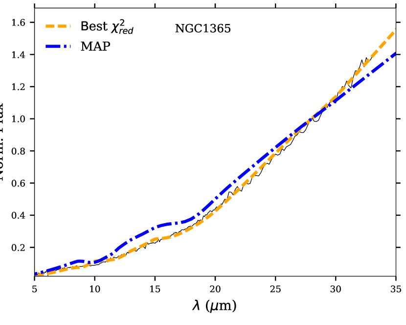
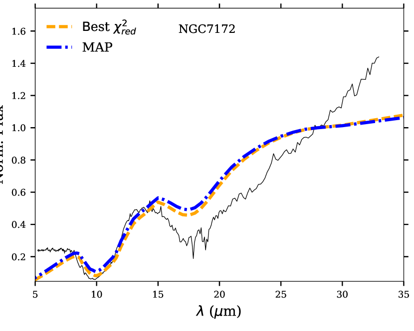
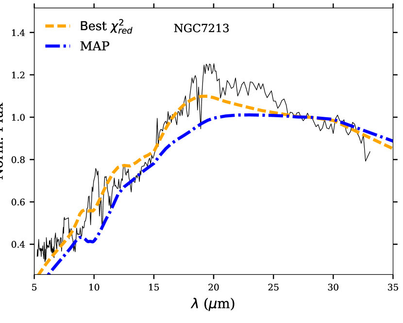
Figure 4: Examples of adjusts for the best fit using ${\chi_{red}}^{2}$ and the maximum-a-posteriori distribution from BayesCLUMPY. Best torus fitting to the spectrum is represented by yellow dashed line for the former and by blue dotted-dashed line in the latter case. The observed spectra and the SED models are normalized at 28$\mu$m.

We apply the Bayesian inference tool BayesCLUMPY (Asensio Ramos & Ramos Almeida, 2009) in order to achieve the best fitting parameters for the observed nuclear SEDs. The technique consists to perform a Markov Chain Monte Carlo method to investigate the parameter space defined by the first 13 eigenvectors. These values result from the combination of the principal component analysis and the artificial neural network that provides a interpolation in the database of the model grid from the theoretical clumpy models ($\sim 10^{6}$ models). This approach allows to obtain the marginal posterior distribution for each model parameter, taking into account all a-priori constrains and the information from the observations. To assure the stability of the solution, we performed consecutive runs of the algorithm. It is important to emphasize that fitting clumpy torus models to the spectra is an intrinsically degenerate problem, as we can obtain the same observable effect for different sets of parameters.

3.2.3 Final Fitting

An example of fitting for some galaxies is presented in Figure 4 and the individuals fittings are presented in the Appendix C. The yellow dashed line shows the model fitted for the minor ${\chi_{red}}^{2}$ value, e.g., the best fit, and blue dotted-dashed line represents the correspondent best $\chi^{2}$ solution for BayesCLUMPY inference, the maximum-a-posteriori (MAP) values. The derived mean parameters for both $\chi^{2}_{red}$ and the Bayesian method are very similar, and in general the $\chi^{2}_{red}$ solution is the most approximated to the observed spectrum (besides that it provides a solution within the models base). The goodness of both fitting procedures can be quantified by the values derived for the $\chi^{2}_{red}$. We also account an additional quality indicator, the adev, which gives the percentage mean deviation over all fitted wavelengths (Cid Fernandes et al., 2013):

$${adev}=\frac{1}{N}\sum_{i=1}^{N}\frac{|F_{obs,\lambda_{i}}-F_{mod,\lambda_{i}}|}{F_{obs,\lambda_{i}}}$$ (4)

In Figure 5 we present the distribution of the adev and the minimum $\chi^{2}_{red}$ values derived for all the sample (except for the galaxies Mrk 3, NGC 1097, NGC 1566, NGC 4594, NGC 5033 and NGC 7679 that present values $\chi^{2}_{red}$ and MAP$>$50). For more than 50% of the adjusted models we found $\chi^{2}_{red}$ values less than 5, which can be classified as satisfactory adjustments. Also, the deviation between the observation and the best model fitted is less than adev$\lesssim 20$% for the majority of objects. In general, the Figures 4 and 5 indicate that the $\chi^{2}_{red}$ method provides more satisfactory adjusts than the MAP using the BayesCLUMPY. This is the reason we have chosen to only discuss the $\chi^{2}_{red}$ results in the next sections.

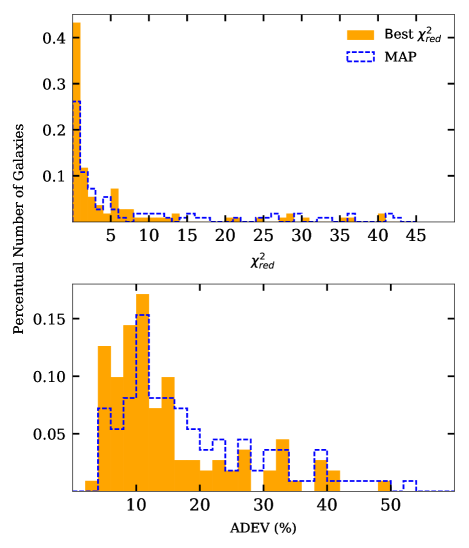
Figure 5: We show the values derived for the $\chi^{2}_{red}$ (top panel) and the adev (bottom panel) that quantify the goodness of the $\chi^{2}_{red}$ and the BayesCLUMPY fitting techniques. The orange filled histograms represent the values derived using the $\chi^{2}_{red}$ technique while the blue dashed lines are the distribution of the MAP values derived using the BayesCLUMPY method.

4 Comparison between type 1 and type 2 sources

In order to compare the two fitting methodologies, we decided to consider the best solution of the ${\chi_{red}}^{2}$ test and the MAP provided by the BayesCLUMPY method. However, it is important to notice that the model interpolations performed in BayesCLUMPY allows for a grid of parameters different from the ones provided by the clumpy torus models and listed in Table LABEL:obs:tab2.

4.1 Direct Parameters

Both fitting methodologies allows for the determination of parameters within the models set, what we call direct parameters. The values obtained for those parameters are presented in frequency histograms (Figure 6) as well as, the obtained mean parameters are listed in Table LABEL:obs:tabmean. We have chosen to discuss the results obtained with the ${\chi_{red}}^{2}$ methodology, however, for completeness we will keep in all the histograms the results obtained with the BayesCLUMPY MAP mode. Below we discuss the results of each parameter individually.

It can be seen from Figure 6 that the inclination angle relative to the observer’s LOS, $i$, appears to be larger for Sy 2 ($\rm\bar{i}(Sy2)=64.5^{\circ}\pm 28.3^{\circ}$) than for Sy 1 ($\rm\bar{i}(Sy1)=50.6^{\circ}\pm 31.4^{\circ}$). This parameter was studied in previous works, with controversial results. RA11 studying a sample of 7 Sy 1 and 14 Sy 2 galaxies and from the 13 objects presented in AH11 sample, found no significant differences in this parameter and suggested that type 2 objects could be seen in any orientation if there is at least one cloud obscuring the observers LOS. On the other hand, Mor, Netzer & Elitzur (2009) studied 26 type 1 PG quasars using Spitzer data found $\bar{i}$=33^∘ while Lira et al. (2013) obtained a typical value of i $\gtrsim$40 for a sample of 27 Sy 2 with about half of their sample requiring values $i\sim$70-90^∘. Our mean results for this parameter suggest that Sy 1 do present a slightly lower value for $i$ than Sy 2s, supporting the viewing angle orientation requirement for the AGN’s Unified Model.

Table 2: Mean parameters derived from the ${\chi_{red}}^{2}$ and MAP of CLUMPY models fitting

Parameter	$\chi^{2}_{red}$	MAP
	sy 1 — sy 2	sy 1 — sy 2
Direct
i	50.6$\pm$31.4 — 64.5$\pm$28.3	57.1$\pm$32.7 — 51.6$\pm$35.3
$\sigma$	36.4$\pm$19.2 — 43.7$\pm$20.5	44.7$\pm$19.8 — 50.7$\pm$17.6
N	9.0$\pm$5.0 — 10.0$\pm$4.0	8.0$\pm$5.0 — 11.0$\pm$5.0
Y	53.7$\pm$34.9 — 46.1$\pm$34.1	54.5$\pm$34.9 — 53.1$\pm$38.3
$\tau_{V}$	77.3$\pm$57.0 — 110.9$\pm$49.2	69.5$\pm$52.2 — 93.0$\pm$52.1
q	0.8$\pm$0.8 — 0.9$\pm$0.7	1.0$\pm$0.8 — 0.8$\pm$0.8
Indirect
Nlos	3.0$\pm$4.0 — 7.0$\pm$5.0	4.0$\pm$4.0 — 6.0$\pm$5.0
AV	287$\pm$595 — 899$\pm$829	241$\pm$509 — 671$\pm$799
log($N_{H}/\rm cm^{-2}$)	23.7$\pm$24.1 — 24.2$\pm$24.2	23.7$\pm$24.0 — 24.1$\pm$24.2
Pesc	0.3$\pm$0.3 — 0.1$\pm$0.2	0.2$\pm$0.3 — 0.1$\pm$0.2
CT	0.7$\pm$0.2 — 0.8$\pm$0.2	0.8$\pm$0.2 — 0.9$\pm$0.2
$M_{tor}(M_{\odot})$	2.1$\pm$3.9$\times$106 — 2.7$\pm$5.5$\times$106	2.4$\pm$3.7$\times$106 — 3.5$\pm$6.0$\times$106

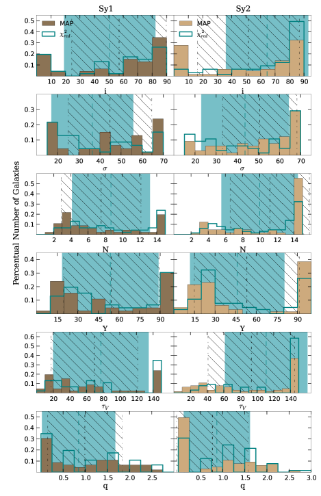
Figure 6: The frequency histograms distribution for direct parameters, $\rm i$, $\rm\sigma$, $\rm N$, $\rm Y$, $\rm\tau_{V}$ and $\rm q$, derived from the clumpy models fitting. The brown filled histograms represent the MAP distributions resulting from the employing of the BayesCLUMPY task and the stepped blue distribution shows the results of the best solution applying the $\chi^{2}_{red}$ test. In all panels, the distributions for the 46 Sy 1 are plotted at the left side and for the 65 Sy 2 at the right side. The lined-dotted lines indicate the mean value of the MAP distribution and the hatched area delineate the mean values from the $\chi^{2}_{red}$ and the uncertainties around the average.

Accordingly the clumpy models, the dusty clouds follow a Gaussian like distribution along the equatorial ray characterized by a torus angular width ($\sigma$). Our results show that there is no significant differences for the mean $\sigma$ values in the different types of activity, being $\rm\bar{\sigma}(Sy1)=36.4^{\circ}\pm 19.2^{\circ}$ and $\rm\bar{\sigma}(Sy2)=43.7^{\circ}\pm 20.5^{\circ}$. Taking only the mean values into account, these results may indicate that the torus hosted by Sy 1s is biased towards smaller values than those found in Sy 2s. In fact, these values agree with those found by RA11 and are further supported by the findings of Lira et al. (2013, $\sigma>$ 40, for 70% of their Sy 2) and Mor, Netzer & Elitzur (2009, $\bar{\sigma}=34$, for their type 1 sources). Regarding the number of clouds along the LOS, we found that both types are well represented by $\sim$ 10 clouds ($\rm\bar{N}(Sy1)=9\pm 5$ and $\rm\bar{N}(Sy2)=10\pm 4$). In the case of quasars this number seems to be smaller ($\sim$5)than in the case of Seyfert galaxies (e.g Mor, Netzer & Elitzur, 2009; Lira et al., 2013). Thus, our findings reinforce the scenario proposed by AH11 in which the number of clouds might be in an evolutionary stage of a receding torus.

Besides the above parameters, other fundamental parameter is the torus thickness, $Y$, which is calculated as the ratio of the outer $\rm R_{o}$ and inner radius $\rm R_{d}$, $\rm Y=R_{o}/R_{d}$, where $\rm R_{d}$ is set as being the distance from the central source where dust sublimates and according to Barvainis (1987) can be obtained by

$$R_{d}=0.4{\left(\frac{L_{AGN}}{10^{45}\rm erg^{-1}}\right)}^{0.5}{\left(\frac{1500\rm K}{T_{sub}}\right)}^{2.6}\leavevmode\nobreak\ \leavevmode\nobreak\ \rm pc$$ (5)

with $\rm T_{sub}$ being the dust sublimation temperature and $L_{AGN}$ is the AGN bolometric luminosity. The values we derived for the torus thickness do not present any significant distinction on average values and also for the shape of the distribution, as it can be seeing in Figure 6. For both classes, we can find solutions at the edges of the distribution, indicating that the majority of objects requires or a very large value of Y or a compact torus. In this case, the mean values derived ($\rm\bar{Y}(Sy1)=53.7\pm 34.9$ and $\rm\bar{Y}(Sy2)=46.1\pm 34.1$) do not represent the sample.

In fact, as pointed out by Nenkova et al. (2008b), when $q=2$ the IR fitting leads to a poor constrain on the torus extension, since the clouds are distributed close to $R_{d}$. Therefore RA11 and AH11 have chosen to restrict this parameter accordingly with observations that suggest smaller values for the torus radial extension ( Y$\sim$10-20, Jaffe et al., 2004; Tristram et al., 2007; Raban et al., 2009). We also performed our MIR fitting using the same constrain of Y[5,30] adopted in AH11 and still our findings do not imply significant changes on the other parameters distribution. Hence, we decided to maintain the original $Y$ parameter space since this bi-modality found in our results can be attributed to a better constrain on $\gtrsim$20 $\mu$m which are not included to the SEDs in the AH11 and RA11 sample. Indeed, Fuller et al. (2016) shows that the inclusion of SOFIA photometric data in the 30-40 $\mu$m wavelength range helps to better constrain $Y$. This is because the outer radius $R_{o}$ is more sensitive to the cooler dust that peaks in the far-IR, providing information about the torus size.

Due to computational limitations, the clumpy models assume that all dust clouds have the same optical depth, $\tau_{V}$ (see Nenkova et al., 2008b, for details). It is clear from Figure  6 that the distribution of individual clouds optical depths points is centred in high values of $\tau_{V}$. Also, approximately 60% of the solutions for Sy 2 galaxies require $\tau_{V}\sim 140$ mag, presenting an average value of $\rm\bar{\tau_{V}}(Sy2)=111\pm 49$ mag for type 2 sources, while for Sy 1 we found a smaller value for $\rm\bar{\tau_{V}}(Sy1)=77\pm 57$ mag. Both results are in agreement with the high optical depth condition ($\rm\tau_{V}\gtrsim 60$) of the clumpy models, which requires such values to ensure that we do have optically thick clouds and a finite photon escape probability. However, for this parameter, our results differ from those found in the literature, which derive lower values of $\tau_{V}$ for Sy 2 galaxies, for example, for the 14 Sy 2 sample of RA11 the typical values derived are $\tau_{V}\sim 30$ mag and for the 27 Sy 2 from Lira et al. (2013), the best solutions in general assume lower values ($\tau_{V}\lesssim 25$ mag). We also tested for a possible correlation with $\tau_{V}$ and the galaxy inclination and no correlation was found.

In the clumpy model the clouds distribution is described by a power law with form $r^{-q}$. The histograms with the indexes ($q$) distribution for both types of activity show that the solutions are found to be more likely within lower values for this parameter, generally between $0<q<1$. Values of $q\sim 0$ indicate a constant distribution, revealing that the number of clouds presents a weak dependence on the distance to the central AGN, while values $q\sim 1$ point to a distribution following a $1/r$ relation. The average values derived for both classes are quite similar for both types of activities, being $\rm\bar{q}(Sy1)=0.8$ and $\rm\bar{q}(Sy2)=0.9$. Our results follow the same trend as found by Mor, Netzer & Elitzur (2009, $\bar{q}=1$) and also by Lira et al. (2013, $\rm q\sim 0$), since the distribution for this parameter is quite spread as can be seen in the histograms in Figure 6, where more than 30% of the sample present values of $q=0$.

Table 3: The K-S test for the parameters distribution of Sy1 and Sy2

Parameter Distribution	D	p-value
i	0.44	0.25
$\sigma$	0.18	0.99
N	0.33	0.31
Y	0.20	0.97
$\tau_{V}$	0.27	0.59
q	0.17	0.99

We also performed a two-sample Kolmogorov-Smirnov (K-S) test (Mises, 1964) in order to verify the results discussed above and quantify the differences between the parameters distribution for both activity types. The K-S test determine if the Sy 1 and Sy 2 parameters have the same distribution and the values derived for $D$, i.e. the supremum of the cumulative distribution functions (CDFs) of the Sy 1 and Sy 2 for each clumpy parameter, and $p$-$value$ are shown in Table LABEL:ks_tab. As we can see, the inclination $i$ presents a significant discrepancy between the CDFs since the $D$ value is the most considerable among the other clumpy parameters, followed by $N$ and $\tau_{V}$. Since in both activity types we found $N\sim$10, the main parameters to classify a Sy 1 or a Sy 2 rely on a combination of $i$ and $\tau_{V}$: it depends on the observers’ LOS orientation as well on the obscuring properties of the clouds. On the other hand, the $p$-$value$ for $\sigma$, $Y$ and $q$ suggest that Sy 1 and Sy 2 populations are drawn from the same distribution, e.g., we can not distinguish whether a distribution of the geometrical parameters $\sigma$, $Y$ and $q$ is from a Sy 1 or a Sy 2.

Some objects in our sample are common to previous works of RA09 (9 objects), AH11 (14 objects), RA11 and Lira et al. (2013) (20 objects). In general, our mean results are in good agreement with the literature, although the individual solutions may be quite different. We attribute these differences to the fact that each study used distinct approaches (for example, wavelength coverage, resolution, parameter constrains, methodology). For instance, that may also explain the differences in the reported parameters for the same galaxy in different papers by the same authors. In addition, our results in general tend to be more consistent with those presented by Lira et al. (2013). As pointed out by the latter, there are very significant differences in the results found between RA11 and AH11 attributed to the inclusion of the 10 $\mu$m spectroscopic observations. Since the silicate at 9.7 $\mu$m is a important dust feature, the inclusion of detailed spectral information around this feature is crucial to properly describe the physical parameters from the SEDs.

In order to illustrate a mean SED and torus physical representation, we present a sketch in Figure 7 that shows the mean theoretical SEDs from clumpy to create a representative SED for each type of activity. There we combine the mean parameters derived in Table LABEL:obs:tabmean. We also illustrate a schematic cross section view of the tori for both activity types, in order to highlight the differences in the torus physical properties, for instance, the slightly larger radial thickness for Sy 1 and the wider angular width in Sy 2, consequently, (given the Gaussian distribution) increasing the number of clouds in this type. These results are in agreement with the results of RA11 who found that the tori of Sy 1’s are narrower and with fewer clouds than those found in Sy 2’s. Furthermore, the mean SEDs do not present a turnover of the torus emission, predicted to occur between 30 - 50 $\mu$m. This result is in agreement with those found by Fuller et al. (2016), where no turnover was observed below 31.5 $\mu$m. Further nuclear far-IR observations would be essential to determine the peak of the IR emission, giving insight into the torus outskirts.

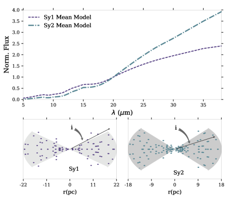
Figure 7: Combination of the mean parameters from clumpy theoretical SEDs, represented by the dashed purple line for Sy 1 and the dotted-dashed blue lines for Sy 1. A schematic torus cross section is also illustrated in order to feature the main differences between the torus physical properties.

4.2 Indirect Parameters

As mentioned before, the model geometry enable us to estimate other important parameters that may help us to understand the physical properties of the putative torus required by the unified model. The distribution derived for the indirect parameters are described below and presented in Figure 8 as well as the information about mean values are summed up in Table LABEL:obs:tabmean and described in the text. It is worth mentioning that all these indirect parameters where obtained using the results of the best direct parameters described in the previous section.

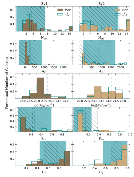
Figure 8: The frequency histograms distribution for indirect parameters, $N_{los}$, $A_{V}$, $N_{H}$, $P_{esc}$ and $C_{T}$, derived from the clumpy models fitting. The brown filled histograms represent the MAP distributions resulting from the employing of the BayesCLUMPY tool and the stepped blue distribution shows the results of the fit best solution applying the ${\chi_{red}}^{2}$ method. The panels follow the same scheme listed in Figure 6.

Since we are dealing with a clumpy media one of the most important parameters in describing the torus is the number of clouds blocking our LOS ($N_{los}$). By using the model clouds distribution (with a Gaussian like form), centred at the equatorial plane, we can compute the number of clouds along any specific direction, thus if we choose the LOS direction we can compute $N_{los}$ (Equation 1). The $N_{los}$ distribution is shown in the top panel of Figure 8, by inspecting this figure, it is clear that the number of clouds along the observer’s LOS presents a sharp peak in its distribution for Sy 1 (centred at $\sim$3), while a spread distribution is found for Sy 2 ($\bar{N_{los}}=7$). At the same level of importance, is the extinction of the light caused by the material composing the LOS clouds. Once $N_{los}$ is know the total optical depth along the LOS is obtained with Equation 2. The distribution of A_V is well defined for Sy 1, with small values, while in Sy 2 it is flat. In addition, the determination of $N_{los}$ is also related with the X-ray columnar hydrogen density which can be derived using the standard Galactic ratio and the foreground extinction from Bohlin, Savage & Drake (1978) via $N_{H}/A_{V}$=1.9$\times$10${}^{21}\rm cm^{-2}$. In agreement with the two previous indirect parameters, the $N_{H}$ is well defined for the Sy 1 galaxies ($\bar{N_{H}}=5\times 10^{23}cm^{-2}$) and with a not so centred distribution for Sy 2’s ($\bar{N_{H}}=1.6\times 10^{24}cm^{-2}$).

These results together with the fact that we are not finding significant difference in the observers viewing angle for the different classes, point to the fact that the most important parameter in determining if a galaxy is classified as a type 1 or 2 object is if there are clouds able to block the radiation from the BLR and central engine. This suggests that the fundamental requirements of the unified model for AGNs depends more on the intrinsic parameters of the torus than on its geometry. In fact, our results are still supported by the finding of RA11 found significant differences in the torus angular size for the different classes. However, in contradiction with our results, they do find lower optical depth in Sy2 when compared with Sy 1.

One of the fundamental requirements of the unification schemes is if a photon generated in the accretion disk is able to scape through the torus. Thus, a fundamental parameter that can be derived from Nenkova et al. (2008b) formalism is the escape probability, $P_{esc}$. This parameter can work as a estimator whether an object is type 1 or type 2, since the putative large viewing angles in the latter is associated with the probability to have more clouds blocking the AGN radiation, leading to a finite but small probability of direct view to the AGN. When the condition $\tau_{V}\gg$1 is achieved $P_{esc}$ can be estimated as:

$$P_{esc}\cong e^{-N_{los}}$$ (6)

The frequency histograms showing the $P_{esc}$ are presented in Figure 8. The results agree with the predictions (i.e. lower probabilities are expected in type 2 objects). We found mean values of $\rm\bar{P}_{esc}(Sy2)=0.1$ and $\rm\bar{P}_{esc}(Sy1)=0.3$ indicating that, on average, a photon originated in the central source has a $\sim$30% chance to escape from the torus without being absorbed. The individual clouds emission, as adopted in the clumpy models formalism, plays a fundamental role to understand the emerging IR torus radiation. It can be originated by clouds directly illuminated by the AGN photons plus the reprocessed radiation from the shaded side of clouds which are heated by the emission of more internal clouds. Thus, what is observed is a sum of the radiation emitted by the torus and the photons generated in the accretion disc that are able to scape (i.e. $P_{esc}$), therefore knowing $P_{esc}$ is fundamental to determine the whole SED emission.

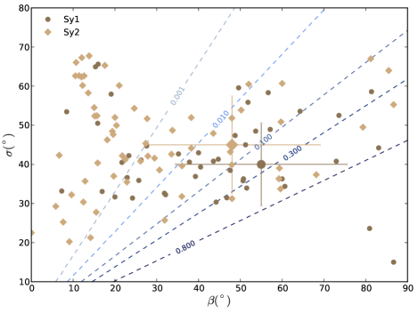
Figure 9: The figure illustrates the distribution of $P_{esc}$, the photon escape probability, in function of the torus width, $\sigma$ and the complementary viewing angle, $\beta$=$\pi/2-i$, related by Equation 6. In agreement with the unified model premise, which expect that Sy 2 galaxies more likely on the left side and Sy 1 on the center of the graph and higher $P_{esc}$ values, we found Sy 2 more concentrated at lower probabilities, except for some objects. As a representative value for our sample, we utilized $N$=10 to plot the $P_{esc}$ curves.

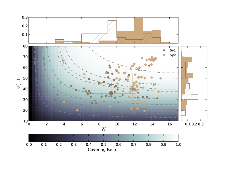
Figure 10: The graph represents the distribution of $N$ and $\sigma$ and their correlation with the covering factor, $C_{T}$. Covering factors curves are present for values from 0.2 to 0.9 according to Equation 7. The closed diamonds represent the Sy 1 objects and the circles show the Sy 2 types. The histograms for $N$ and $\sigma$ are attached at the top and right side of the main plot, respectively, for both activity types. As argued in Elitzur (2012), the Sy 2 galaxies are more likely drawn from the distribution of higher covering factors than Sy 1 types.

Once $P_{esc}$ is a non-linear function of $\sigma$, $\beta$ and $N$ we used the results we obtained with our Spitzer data fittings for $\sigma$ and $\beta$ and adopted a value for $N$=10 in order to determine $P_{esc}$ curves in the $\sigma\times\beta$ plane. The results are shown in Figure 9, for display purposes for this figure we used a 10% of $\chi^{2}_{red}$ deviations as described in Sales et al. (2013). It emerges from this figure that most of the Sy 2 galaxies present $P_{esc}\lesssim$10%. The distribution of $P_{esc}$ is quite broad for Sy 1, that may be a reflect of the fact that both $\sigma$ and $\beta$ do present a variety of values in this class (see Figure 6). This parameter was also studied by RA11 and AH11, our results are in good agreement with those found by these authors, in the sense that there is a significant difference between both types of activities. However, while we find almost the same fraction for Sy 1s, we find larger values for Sy 2s than the values found by these authors. We attribute this difference (in type 2 objects, $P_{esc}^{we}$=10% and $P_{esc}^{they}$=0.1%) to the fact they restricted the torus thickness (5$\leq$ Y $\leq$ 30) and we allow it to take all the possible values.

Another parameter provided by the model is the geometrical covering factor that can be understood as the sky fraction at the AGN centre which is being obscured by the dusty clouds. This parameter can be determined by integrating the $P_{esc}$ over all orientations, following the equation (Nenkova et al., 2008a):

$$C_{T}=1-\int_{0}^{\pi/2}P_{esc}(\beta)\cos(\beta)d\beta$$ (7)

The distribution of the derived values for $C_{T}$ are presented in Figure 8. We found slightly larger $C_{T}$ values for type 2 sources ($\rm\bar{C}_{T}(Sy2)=0.8\pm 0.2$) than for type 1 galaxies ($\rm\bar{C}_{T}(Sy1)=0.7\pm 0.2$). Our values are in agreement with literature in the sense that there is a difference between both activities, however, while RA11 find typical values of 0.5 for for the Sy 1 in their sample, these authors find almost the same values we found for the Sy 2 in their sample. Mor, Netzer & Elitzur (2009) also found an even smaller ($\sim$0.3) mean value in their type 1 PG quasars sample.

Accordingly to Nenkova et al. (2008a) the definition of $C_{T}$ arises from the geometry and probabilistic nature of a clumpy medium and can be interpreted as the fraction of randomly distributed observers whose view to the central source is blocked, or as the fraction of type 2 objects in a random sample. The covering factor can be also decisive into AGN classification, because an AGN with a larger covering factor has a higher probability to be viewed as type 2. Many questions are still opened concerning the definition of the intrinsic covering factor, if the geometrical one is related with the “dust” covering factor proposed by Maiolino et al. (2007) (defined as the ration between the thermal component and the AGN contributions). Since the covering factor measures the fraction of AGN luminosity captured by the torus and converted to infrared, the AGN IR luminosity is $C_{T}L_{bol}$, where $L_{bol}$ is its bolometric luminosity (Elitzur, 2012). Thus, it is expected that type 2 AGNs have intrinsically higher IR luminosities than type 1. However, in disagreement with earlier expectations of a strong anisotropy at $\lambda\lesssim 8\mu$m, Spitzer observations present very similar IR fluxes of type 1 and 2 as shown by Lutz et al. (2004); Buchanan et al. (2006), which can be partly explained by a clumpy torus distribution.

The geometrical $C_{T}$ can be interpreted as the “true” torus covering factor because it is independent on $i$. However, on the other hand, as can be noted from Equation 7 $C_{T}$ depends on N and $\sigma$, thus to investigate this relation we show in Figure 10 the results of the models fits in the $N$–$\sigma$ plane together with the contour plots of $C_{T}$. We found that type 2 objects do preferentially lie on the top right of the figure, or in other words they do have large $C_{T}$ values. However, in the case of type 1 objects (where low $C_{T}$ values are expected, since the BLR emission should be observable) we found that they are spread over the whole plane. AH11 and RA11 suggest that type 1 and type 2 AGNs preferentially are located in different regions on the plane (with type 1 having lower values than type 2), however we do not see this trend in our work because, despite the same results for the $\sigma$, we derived larger values for the number of clouds, $N$, and therefore it is expected more clouds obscuring the central source. Since $C_{T}$ is very sensitive to $N$ and $\sigma$, our results always point to higher values than those found in their sample. We would also like to emphasize that our sample consist in a statistically representing sample, and this trend may be biased since the other works have a smaller sample or due to the restrictions in the parameter space adopted by the authors.

4.3 Torus mass and size

Beside the above torus parameters, the clumpy formalism also allows to determine the mass of the emitting hot dust, as well as to set some constrains on the torus size. From the adjustment of the theoretical SEDs clumpy model, the bolometric luminosity of the AGN, $L_{AGN}$, can be found from the scale factor ($\Theta$) of the model to the observation, by solving the equation:

$$\lambda_{obs}F_{obs,\lambda}=\Theta\frac{\lambda_{mod}F_{mod,\lambda}}{F_{AGN}}$$ (8)

We can derived $L_{AGN}$ applying the distance relation $L_{AGN}=4\pi D^{2}\Theta$ and once it is calculated Equation 5 can be used to estimate the inner radius, assuming a sublimation temperature for the silicate grains (we used $T_{sub}=1500$ K). The torus dimension is estimate by the relation Y=$R_{o}/R_{d}$, where $Y$ is taken from the best fit. In order to test the $L_{AGN}$ values derived from the scaling of the clumpy models, we can compare them with those reported in the literature for the X-rays by applying the bolometric correction of $\sim$20 (Elvis et al., 1994) and the comparison between the fitted and literature $L_{AGN}$ is shown in Figure 11. As can be seen from the one-to-one line the observed and calculated values do agree well.

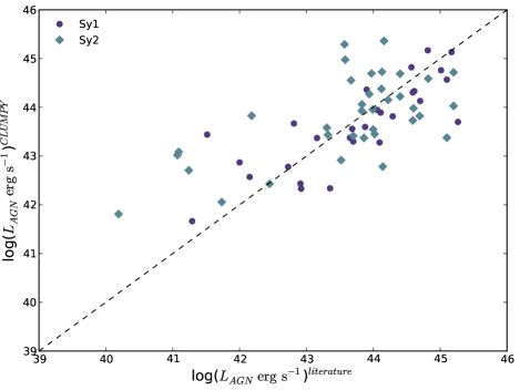
Figure 11: Comparison between the bolometric luminosities, $L_{AGN}$, derived from the clumpy models with those reported on the literature for the hard X-ray luminosities, $L_{X}$, applying the bolometric corrections of Elvis et al. (1994). The diamonds represent the Sy 1 objects while the circles indicate the Sy 2 types and the dashed line indicates the identity line.

Figure 12 shows histograms for the distributions of $L_{AGN}$ and $R_{o}$. No significant differences between type 1 and type 2 galaxies are seen. In general, the estimated values of the AGN bolometric luminosity range between $42<log(L_{AGN})<46$, and the average values in both classes are typically $L_{AGN}\sim 10^{44}$. For the sublimation radius we find averages $\rm R_{d}(Sy1)=$0.12 pc for Sy 1 galaxies and $\rm R_{d}(Sy2)=$ 0.16 pc for Sy 2, which lead to average torus sizes very close to those found in the literature (RA09, AH11, RA11, Lira et al., 2013), with typical values of $R_{o}\lesssim$6 pc. These results are further supported by observational evidences. For instance, previous works using MIR interferometric observations provide information of a relatively compact torus, with a few parsecs scale (Jaffe et al., 2004; Tristram et al., 2007, 2009; Burtscher et al., 2009).

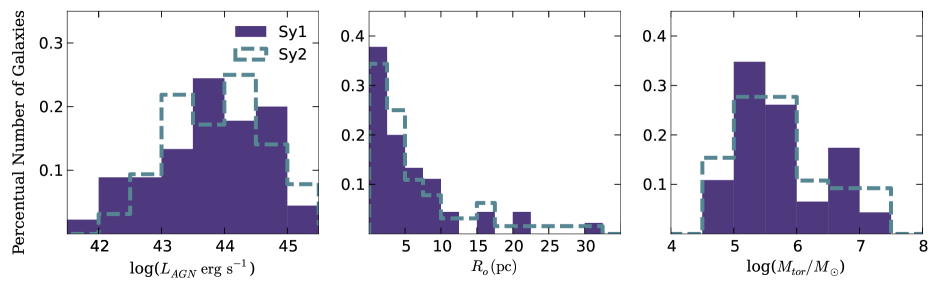
Figure 12: The histograms show the distribution of the AGN bolometric luminosities (left panel), torus sizes, $R_{o}$, in the middle panel and the torus masses, $M_{tor}$ at the right. Histograms filled in purple represent the distributions for Sy 1 and dashed lines in blue indicate the distributions for Sy 2.

By adopting some approximations for the torus geometry and size, we can also estimate its total mass. Considering the mass of a single cloud as $m_{H}N_{H,c}A_{c}$, where $N_{H,c}$ is its column density and $A_{c}$ its cross sectional area, the total mass in clouds is given by $M_{tor}=m_{H}{N_{H}}^{1}\int\eta_{c}(r,\beta)dV$, where $\eta_{c}(r,\beta)$ indicates the clouds distribution profile. For simplicity, assuming a sharp-edge angular distribution, $M_{tor}$ can be analytically calculated (Nenkova et al., 2008b):

$$M_{tor}=4\pi m_{H}sin(\sigma){N_{H}}^{(eq)}R_{d}^{2}YI_{q}(Y)$$ (9)

where $Y_{q}=$1, $Y/(2lnY)$ and $Y/3$ for $q=$2,1 and 0, respectively, and ${N_{H}}^{(eq)}$ is the mean overall column density in the equatorial plane. The latter can be estimated by multiplying the number of clouds along the equatorial ray $N$ by a single cloud columnar density $N_{H,c}$ $\sim$10²²–10${}^{23}\rm cm^{-2}$. Finally, since $N\sim$ 5–15,${N_{H}}^{(eq)}$ assumes typical values of $\sim$10²³–10${}^{24}\rm cm^{-2}$.

We found that $M_{tor}$ ranges from $\rm 10^{4}M_{\odot}$ to $\rm 10^{7}M_{\odot}$ in both activities with mean values typically with $\rm 10^{6}M_{\odot}$ (Figure 12), in agreement with the estimating by Lira et al. (2013) and Mor, Netzer & Elitzur (2009) using the clumpy model formalism to derive $M_{tor}$. A recent work from García-Burillo et al. (2014) was able to constrain $M_{tor}$ derived from clumpy models fitting with the mass of molecular outflow observations in NGC 1068 using ALMA observations in band 7 and 9. They estimate $M_{tor}\sim 2\times 10^{5}M_{\odot}$, consistent to the estimated molecular gas mass detected inside the central aperture (r=20 pc) derived from the CO(3-2) emission.

5 The effects of hot dust emission

It is widely known that the inner torus radius is related with the dust grains sublimation temperature ($T\sim$800-1500 K). Such temperature peaks at NIR wavelengths and in the case of AGNs this emission is related with the dusty torus (Barvainis, 1987; Rodríguez-Ardila & Mazzaly, 2006; Riffel et al., 2009). Therefore, the inclusion of the NIR spectral region is crucial to probe the hotter and innermost regions of the torus.

In fact, Ramos Almeida et al. (2014) demonstrated the need of the inclusion of the NIR data to constrain the torus parameters, especially to constrain the torus radial extension, Y. In their work, they analysed a compilation from the literature of NIR+MIR photometry and MIR spectroscopy (8-13$\mu$m) of six Seyfert galaxies. All the objects in their study share the same characteristics: undisturbed, face-on galaxies with no prominent emission of dust lanes. In particular, they recommend a minimum combination of data in the $J$+$K$+$M$- band photometry and the $N$-band spectroscopy.

In order to study the effects of the hotter and inner region of the torus we included in our analysis $ZJHK$-band long-slit spectroscopy data, for the 32 objects where such information was available in the literature. Data for 24 galaxies were obtained from Riffel et al. (2006). These data where collected using the SpeX spectrograph of the NASA 3m Infrared Telescope Facility (IRTF) in the short cross-dispersed mode (SXD, 0.8-2.4 $\mu$m) using a slit of 0.8”$\times$15” slit. The used spectra are those of the nuclear extraction (sampling few hundred pc). For more details about the data see Riffel et al. (2006, 2009). The remaining 8 sources were taken from (Mason et al., 2015), these spectra were observed using Gemini telescope GNIRS spectrograph in the XD mode. This instrument also covers simultaneously the 0.8-2.4 $\mu$m wavelength range. The observations where performed using a 0.3”$\times$1.8” slit and the spectral extractions correspond to regions of $\sim$150 to 370 pc in the galaxies. The objects with SpeX or GNIRS spectra available are reported in Table LABEL:obs:tab1 of Appendix A.

The same methodology described in the previous sections was used to perform the fitting of the observed spectra to the theoretical clumpy models. Since both SpeX and GNIRS spectra have higher spectral resolution than the IRS/Spitzer, we rebined the NIR spectra in 0.16$\mu$m intervals in order to have the same sampling as the MIR . The $\chi^{2}_{red}$ minimization was applied once more to all 32 combination of NIR+MIR spectroscopic data. In Figure 13 we present the individual results for each parameter considering all the solutions within 10% deviation of the minimum $\chi^{2}_{red}$ and compare them with the results obtained when using only the Sptizer data.

It is shown that in most of the cases the distribution of Y is well constrain, even when only using the MIR data, despite for some differences for the solution in individual galaxies. The preference for higher values of $\tau_{V}$ can be found in most of the galaxies. We can also notice that the inclusion of NIR data in general better constrain better the torus width $\sigma$. In general, the distribution of the torus parameters using the NIR+MIR combination do not change dramatically compared with those found only using the IRS spectra.

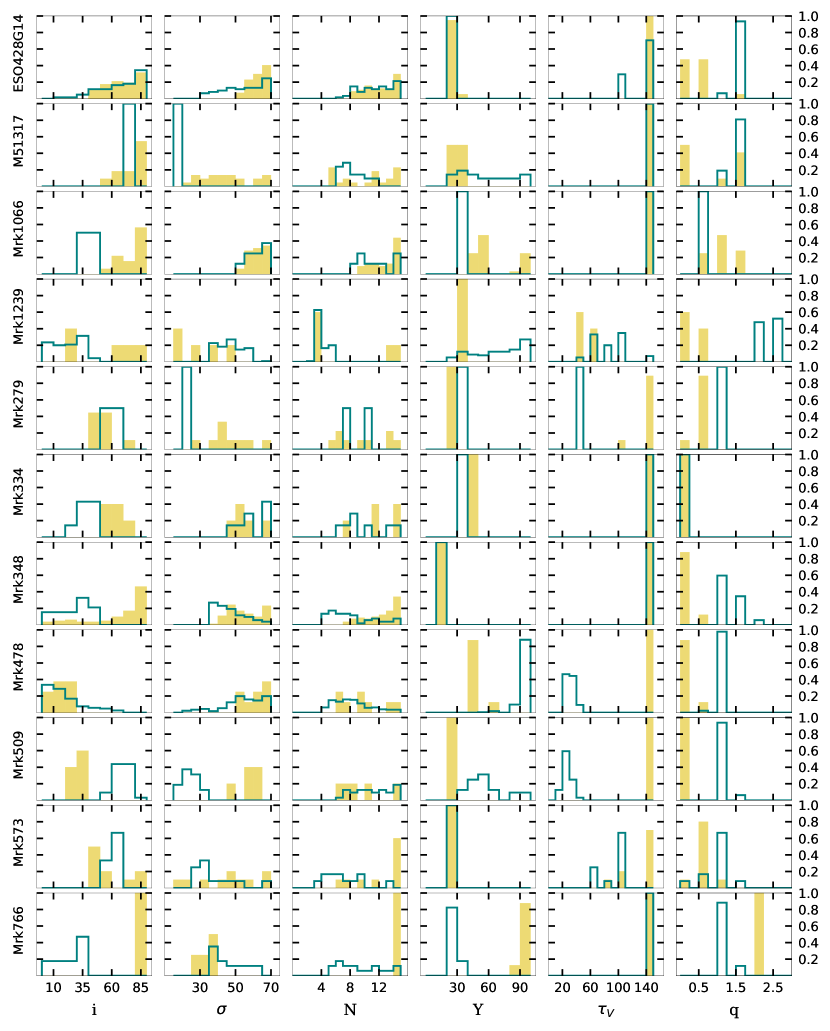
Figure 13: The individual distribution of the six clumpy parameters. The stepped histograms in blue show the parameters distribution of the JHK spectroscopic data and the IRS spectra, while the yellow filled histograms show the results only considering the MIR data.

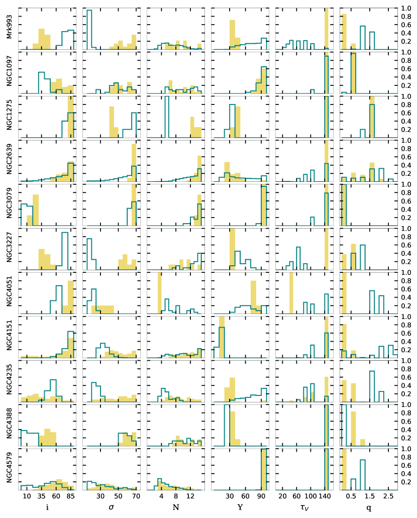
Figure 13: continued from previous page.

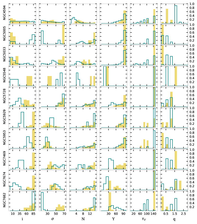
Figure 13: continued from previous page.

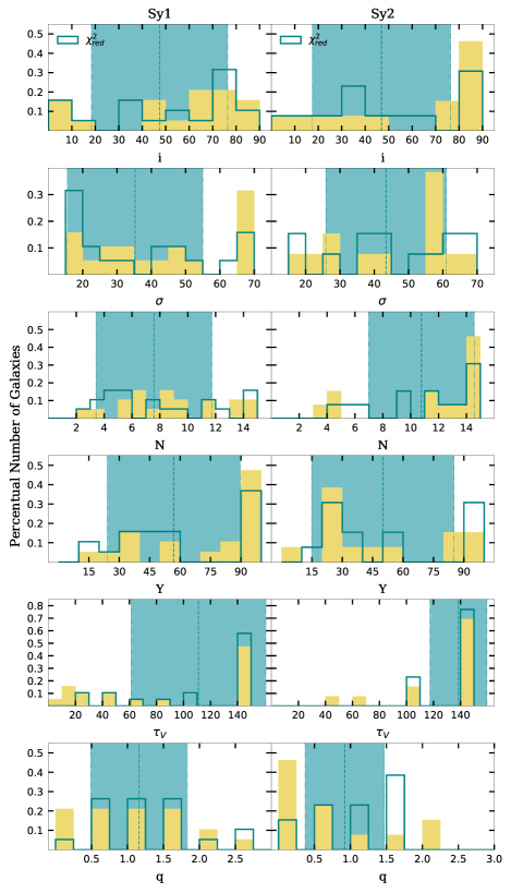
Figure 14: We present the histograms for the distribution of the direct parameters using both NIR+MIR spectra (stepped blue) and compared them with the analysis using the results for the 32 galaxies only considering the MIR data (yellow filled). The distributions for the 19 Sy 1 are plotted at the left side and for the 13 Sy 2 at the right side. The hatched area indicate the mean values from the $\chi^{2}_{red}$ and the uncertainties around the average, represented by the dashed line, for the NIR+MIR combination.

Following the previous methodology, in order to study the main differences between type 1 and type 2 objects, we compared the mean results for the 19 Sy 1 and 13 Sy 2, as shown in Figure 14, obtained by including the near-IR spectral range with that obtained if we only consider the MIR data. The only noticeable change is found for the clouds’ radial profile for Sy2’s, where slightly higher values ($q\sim$1.5) are found when including the NIR spectral range in the analysis.

The inclusion of the NIR to our analysis does reinforce our previous results, that the inclination angle to the observer is not the only relevant parameter to distinguish between the galaxy type. Instead, the combination of the observer’s angle, the number of clouds and the physical properties of the clouds, described by the $\tau_{V}$, plays a very important role in the classification. When analysed individually, in general the parameters are well constrained. However, when gathered and compared by type 1 and type 2, we found broad distributions, indicating a large dispersion of the parameters values in each type of activity. The main concern with our findings is the intrinsic degeneracy of the clumpy models, since a combination of different parameters can reproduce almost the same SED.

It is important to remark that the findings of Ramos Almeida et al. (2014) are very relevant in order to constrain all the torus parameters, but they represent a small and very particular sample, without prominent dust emission and face-on galaxies. Our work aimed at exploring the generality of the clumpy models, since they are reproducing only the torus emission and in principle they should represent any galaxy scenario. These results reinforce the fact that we are dealing with the probabilistic nature of a clumpy environment.

We would like to highlight the importance of the use of a large and homogeneous sample in order to the determine in a reliable way the torus properties. One of the main problem when analysing SEDs and the torus properties is that usually data are not uniform. It is common to have a sample of sources in which the data are obtained with distinct filters and instruments (thus probing very different regions of the sources), and in some cases they do not have the same wavelength coverage for each individual galaxy. Consequently, this can lead to different results of the fitting (Ramos Almeida et al., 2014).

6 Conclusions

We proposed to investigate the torus properties in a sample of 46 Sy 1 and 65 Sy 2 galaxies in the Unified Model scenario. The sample consists in all 5-38$\mu$m IRS/Spitzer data available in the heritage archive for Seyfert classification. To isolate the emission from the nucleus, we subtracted the host galaxy contribution in the MIR by removing the PAH bands emission via an IRS spectral decomposing code (pahfit, Smith et al., 2007b).

Recently, many efforts have been made to calculate the torus emission in a clumpiness formalism. One of them are developed by Nenkova et al. (2008a, b) (clumpy models) and here in this work we utilize their $\sim$10⁶ theoretical database models to derive the 6 parameters that better adjust the individual MIR spectra and analyse their distribution.

We found differences in the derived mean values for the observers’ viewing angle, $\bar{i}$=50 for Sy 1 and $\bar{i}$=65 for Sy 2, according to the Unified Model, which suggest that type 2 objects are observed most in edge-on angle views than type 1. Type 2 also appears to be angularly larger, with a mean Gaussian width distribution of $\sigma$=44, while the Sy 1 class present $\bar{\sigma}$=36 and a sightly larger mean torus thickness, $\bar{Y}$=54 ($\bar{Y}$=46 for Sy 2). Despite the fact we found almost the same number of clouds along the equatorial ray, N$\sim$10, the number of clouds obscuring the central source in the observer LOS is, on average, 7 clouds for Sy 2 and $N_{los}\sim$4 clouds in Sy 1, indicating most attenuated SEDs from type 2 sources. The radial index power tends to be more like a flatten radial distribution, with $q\leq$1 in the majority cases, while the $\tau_{V}$ distribution attend the criteria of $\tau_{v}\gtrsim$60 for both types but do present higher values for Sy 2, ($\rm\bar{\tau_{V}}(Sy1)=7$ and $\rm\bar{\tau_{V}}(Sy2)=111$), indicating that the cloud physical properties may be distinct.

The obscuration in type 2 objects requires higher extinction values, with an average value of $A_{V}\sim$900, while for Sy 1 the average found is $\sim$290. The torus masses range from M${}_{tor}\sim$10⁴–10${}^{7}M_{\odot}$ in both cases. Properties derived from de torus symmetry and random distribution nature, $C_{T}$ and $P_{esc}$, where the $P_{esc}$ parameter ensure non-zero AGN probabilities to edge-on inclination, we found about 30% of probability to directly see the central source in type 1 and 10% for Sy 2 in the sample. Geometric covering factors, or the probabilities of absorption by the torus, are in agreement with the prediction for Sy 2, we found that in general 80 per cent of cases the central source is obscured. However, the mean values derived for the Sy 1 ($C_{T}\sim 0.7$) are larger than the values found in previous works (e.g., AH11 and RA11).

We would like to highlight the importance of the use of a large and homogeneous sample in order to the determine in a reliable way the torus properties. In general, the inclusion of $JHK$ spectroscopic data in our MIR sample do not change the global torus properties derived for each type of activity.

Finally, the results follow the orientation dependency suggested by unification schemes, however, some properties concerning the cloud obscuration are not intrinsically the same for both types of activity. The torus geometry and cloud properties, along with orientation effects, may be crucial to characterize the differences between Sy 1 and Sy 2.

On the basis of the presented results, the classification of a Seyfert galaxy may depend also on the dust intrinsic properties of the dusty torus clouds rather than only on the torus inclination angle, in contradiction with the simple geometrical requirements of the putative torus of the unification model.

Appendix A Sample Properties

We present in the following Table LABEL:obs:tab1 the main properties for our 111 Seyfert sample.

Table 4: Sample Properties

Object Name	RA	Dec	z	Distance	Morphological	log(LIR)	L2-10KeV	Active Type	PID
	J2000	J2000		(Mpc)	Type	(L⊙)	(erg $\rm s^{-1}$)
Mrk334†	00h03m09.6s	+21d57m37s	0.022	86.7	Pec	11.02(2)		Sy 1	3374
Mrk335	00h06m19.5s	+20d12m10s	0.026	110.4	Compact	10.72(1)	9.75e+42(6)	Sy 1	3269
Mrk938	00h11m06.5s	-12d06m26s	0.020	84.0	Pec	11.48(1)		Sy 2	3269
E12-G21	00h40m46.1s	-79d14m24s	0.030	128.6	E	11.03(1)		Sy 1	3269
Mrk348†	00h48m47.1s	+31d57m25s	0.015	64.4	SA0/a	10.62(1)	2.47e+43(8)	Sy 2	3269
NGC424	01h11m27.6s	-38d05m00s	0.012	50.4	SB0/a	10.67(1)		Sy 2	3269
NGC526A	01h23m54.4s	-35d03m56s	0.019	81.8	S0 pec	10.78(1)	1.21e+43(6)	Sy 1	86, 3269
NGC513	01h24m26.8s	+33d47m58s	0.020	83.7	Sb/c	10.52(1)	5.25e+42(8)	Sy 2	3269
Mrk993†	01h25m31.4s	+32d08m11s	0.016	60.6	Sa	10.99(4)		Sy 1	40385
Mrk573†	01h43m57.8s	+02d21m00s	0.017	67.4	SAB0	10.48(2)		Sy 2	50094
F01475-0740	01h50m02.7s	-07d25m48s	0.018	75.7	E/S0	10.62(1)	3.31e+43(8)	Sy 2	3269
NGC931	02h28m14.5s	+31d18m42s	0.017	71.3	Sbc	10.92(1)		Sy 1	3269
NGC1056	02h42m48.3s	+28d34m27s	0.005	22.1	Sa	9.93(1)		Sy 2	3269
NGC1097†	02h46m19.0s	-30d16m30s	0.004	17.5	SBb	10.78(1)	7.59e+40(9)	Sy 2	159
NGC1125	02h51m40.3s	-16d39m04s	0.011	46.8	SAB0	10.46(1)		Sy 2	3269
NGC1143/4	02h55m12.2s	-00d11m01s	0.029	123.5	S0 pec	10.46(1)		Sy 2	159
Mrk1066†	02h59m58.6s	+36d49m14s	0.012	47.2	SB0	10.78(2)	8.32e+42(8)	Sy 2	30572
M-2-8-39	03h00m30.6s	-11d24m57s	0.029	128	SABa pec	10.95(1)	7.94e+43(11)	Sy 2	3269
NGC1194	03h03m49.1s	-01d06m13s	0.014	58.2	SA0:	10.34(1)	6.31e+43(11)	Sy 2	3269
NGC1241	03h11m14.6s	-08d55m20s	0.014	57.9	SBb	10.75(1)		Sy 2	3269
NGC1275†	03h19m48.1s	+41d30m42s	0.017	70.9	Pec	11.20(5)	7.24e+42(10)	Sy 2	14
NGC1320	03h24m48.7s	-03d02m32s	0.009	37.7	S0/a	10.21(1)	4.90e+42(8)	Sy 2	159
Mrk609	03h25m25.3s	-06d08m38s	0.034	143	ImPec		6.63e+42(6)	Sy 2	3374
NGC1365	03h33m36.4s	-36d08m25s	0.005	17.7	SBb	11.23(1)	3.25e+41(6)	Sy 1	3269
NGC1386	03h36m46.2s	-35d59m57s	0.003	16.2	Sa,S0	9.53(1)	6.16e+39(6)	Sy 2	3269
F03450+0055	03h47m40.2s	+01d05m14s	0.031	132.8	?	11.10(1)		Sy 1	3269
NGC1566	04h20m00.4s	-54d56m16s	0.005	11.8	SABbc,Sc	10.61(1)	4.17e+41(9)	Sy 1	159
F04385-0828	04h40m54.9s	-08d22m22s	0.015	64.7	S0	10.82(1)	2.00e+43(11)	Sy 2	3269
NGC1667	04h48m37.1s	-06d19m12s	0.015	65.0	SABc	11.02(1)	3.63e+42(8)	Sy 2	3269
E33-G2	04h55m58.9s	-75d32m28s	0.018	77.5	SB0	10.52(1)	4.35e+42(6)	Sy 2	3269
M-5-13-17†	05h19m35.8s	-32d39m28s	0.012	54.1	SB0/a,S0/a	10.28(1)		Sy 1	3269
Mrk3	06h15m36.3s	+71d02m15s	0.0135	55.9	E2 pec	10.78(2)	2.32e+42(6)	Sy 2	14
Mrk6	06h52m12.2s	+74d25m37s	0.019	80.6	SAB0:,Sa	10.63(1)	2.05e+43	(6) Sy 1	3269
ESO428-G014†	07h16m31.2s	-29d19m29s	0.006	26	SAB0 pec			Sy 2	30572
Mrk9	07h36m57.0s	+58d46m13s	0.040	170	S0: pec,SB	11.15(1)		Sy 1	3269
Mrk79	07h42m32.8s	+49d48m35s	0.022	95	SBb,SBc	10.90(1)	2.51e+43(12)	Sy 1	3269
Mrk78	07h42m41.7s	+65d10m37s	0.037	158	SB	11.04(2)		Sy 2	50094
Mrk622	08h07m41.0s	+39d00m15s	0.023	99.6	S0			Sy 2	3374
NGC2622	08h38m10.9s	+24d53m43s	0.029	124	SBb			Sy 1	3374
NGC2639‡	08h43m38.1s	+50d12m20s	0.011	47.7	SAa	10.34(1)	7.08e+40(10)	Sy 1	3269
Mrk704	09h18m26.0s	+16d18m19s	0.029	125.2	SBa	10.97(1)		Sy 1	3269
NGC2992	09h45m42.0s	-14d19m35s	0.008	30.5	Sa pec	10.51(1)	7.20e+41(6)	Sy 1	3269
Mrk1239†	09h52m19.1s	-01d36m43s	0.0199	85.3	E-S0	10.86(1)		Sy 1	3269
NGC3079‡	10h01m57.8s	+55d40m47s	0.004	19.7	SBc	10.62(1)	1.05e+42(8)	Sy 2	3269
NGC3227†	10h23m30.6s	+19d51m54s	0.004	20.9	SABa pec	9.97(1)	2.51e+42(7)	Sy 1	668, 3269
Mrk34	10h34m08.6s	+60d01m52s	0.051	218	Sa	11.15(2)		Sy 2	50094
NGC3511	11h03m23.8s	-23d05m12s	0.004	14.6	SAc	9.95(1)		Sy 1	3269
NGC3516	11h06m47.5s	+72d34m07s	0.009	38.9	SB0	10.17(1)	3.77e+42(6)	Sy 1	3269
M+0-29-23	11h21m12.2s	-02d59m03s	0.025	106.6	SABb	11.36(1)		Sy 2	3269
NGC3660	11h23m32.3s	-08d39m31s	0.012	52.6	SBbc	10.47(1)	7.94e+42(11)	Sy 2	3269
NGC3786	11h39m42.5s	+31d54m33s	0.009	40.9	SABa/Pec			Sy 2	3374
NGC3982	11h56m28.1s	+55d07m31s	0.004	21.8	SABb	9.81(1)	1.41e+41(8)	Sy 2	3269
NGC4051†	12h03m09.6s	+44d31m53s	0.002	17.0	SABbc	9.66(1)	1.64e+40(6)	Sy 1	3269
UGC7064	12h04m43.3s	+31d10m38s	0.025	107.1	SAB	11.18(1)		Sy 1	3269
NGC4151†	12h10m32.6s	+39d24m21s	0.003	20.3	SABab	9.95(1)	2.42e+42(6)	Sy 1	3269
NGC4235‡	12h17m09.9s	+07d11m30s	0.008	38	SAa	10.30(4)	4.07e+41(9)	Sy 1	40936
Mrk766†	12h18m26.5s	+29d48m46s	0.013	55.4	SBa	10.67(1)	6.44e+42(6)	Sy 1	3269
NGC4388‡	12h25m46.7s	+12d39m44s	0.008	18.1	SAb	10.73(1)	3.37e+42(6)	Sy 2	3269
NGC4501	12h31m59.2s	+14d25m14s	0.008	20.7	SAb	10.98(1)	7.76e+38(10)	Sy 2	3269
NGC4507	12h35m36.6s	-39d54m33s	0.012	53	SABab		4.70e+42(6)	Sy 2	30572
NGC4579‡	12h37m43.5s	+11d49m05s	0.005	16.8	SABc	10.17(1)	2.66e+41(6)	Sy 1	159
NGC4593	12h39m39.4s	-05d20m39s	0.009	44.0	SBb	10.35(1)	5.74e+42(6)	Sy 1	3269
NGC4594‡	12h39m59.4s	-11d37m23s	0.003	10.9	SAa	9.75(1)	9.77e+39(9)	Sy 1	159
NGC4602	12h40m36.8s	-05d07m59s	0.008	34.4	SABbc	10.44(1)		Sy 1	3269
Tol1238-364	12h40m52.8s	-36d45m21s	0.011	46.8	SBbc	10.87(1)		Sy 2	3269
M-2-33-34	12h52m12.4s	-13d24m53s	0.015	62.7	Sa	10.49(1)		Sy 1	3269
NGC4941	13h04m13.1s	-05d33m06s	0.004	13.8	SABab	9.39(1)	2.71e+40(6)	Sy 2	86, 3269
NGC4968	13h07m06.0s	-23d40m37s	0.010	42.2	SAB0	10.39(1)		Sy 2	3269
NGC5005‡	13h10m56.2s	+37d03m33s	0.003	17.5	SABbc	10.20(1)	8.71e+39(10)	Sy 2	3269
NGC5033‡	13h13m27.5s	+36d35m38s	0.003	20.6	SAc	10.05(1)	5.01e+40(10)	Sy 1	159
NGC5135	13h25m44.0s	-29d50m01s	0.014	58.6	SBab	11.27(1)	1.26e+43(7)	Sy 2	3269
M-6-30-15	13h35m53.8s	-34d17m44s	0.008	33.2	S?	9.98(1)	6.22e+42(6)	Sy 1	3269
NGC5256	13h38m17.5s	+48d16m37s	0.028	117.3	Pec	11.51(1)		Sy 2	3269
I4329A	13h49m19.2s	-30d18m34s	0.016	68.8	SA0	10.97(1)	7.42e+43(6)	Sy 1	3269
Mrk279†	13h53m03.4s	+69d18m30s	0.030	129	S0	11.90(4)	6.31e+43(12)	Sy 1	666
NGC5347	13h53m17.8s	+33d29m27s	0.008	36.7	SBab	10.04(1)	2.51e+42(7)	Sy 2	3269
Mrk463E	13h56m02.9s	+18d22m19s	0.050	217	S pec	11.70(2)	1.86e+42(6)	Sy 2	105
NGC5506	14h13m14.8s	-03d12m27s	0.006	28.7	Sa pec	10.44(1)	4.99e+42(6)	Sy 2	3269
NGC5548†	14h17m59.5s	+25d08m12s	0.017	73.6	SA0/a	10.66(1)	1.95e+43(6)	Sy 1	86, 3269
Mrk471	14h22m55.4s	+32d51m03s	0.034	147	SBa			Sy 2	3374
Mrk817	14h36m22.1s	+58d47m39s	0.031	134.7	SBc	11.35(1)		Sy 1	3269
NGC5695	14h37m22.1s	+36d34m04s	0.014	60.7	SBb			Sy 2	30773
Mrk477	14h40m38.1s	+53d30m16s	0.038	161	Comp	11.18(2)		Sy 2	30443
Mrk478†	14h42m07.4s	+35d26m23s	0.079	347	S	11.37(3)	5.16e+43(6)	Sy 1	3187, 20142
NGC5728†	14h42m23.9s	-17d15m11s	0.009	41.9	SABa	10.60(5)	1.95e+43(8)	Sy 2	30745
Mrk841	15h04m01.2s	+10d26m16s	0.036	157	E	11.82(4)	3.27e+43(6)	Sy 1	14
NGC5929†	15h26m06.1s	+41d40m14s	0.008	38.5	Sab pec	10.58(1)		Sy 2	3269
NGC5953†	15h34m32.4s	+15d11m38s	0.007	33.0	SAa pec	10.49(1)		Sy 2	3269
M-2-40-4	15h48m24.9s	-13d45m28s	0.025	107.9	Sc	11.32(1)		Sy 2	3269
F15480-0344	15h50m41.5s	-03d53m18s	0.030	129.8	S0	11.14(1)		Sy 2	3269
Mrk883	16h29m52.9s	+24d26m38s	0.037	159	Irr			Sy 2	3374
NGC6810	19h43m34.4s	-58d39m21s	0.007	29.0	SAab	10.74(1)		Sy 2	3269
NGC6860	20h08m46.9s	-61d06m01s	0.015	63.7	SBb	10.35(1)	3.98e+42(12)	Sy 1	3269
NGC6890	20h18m18.1s	-44d48m25s	0.008	31.8	SAb	10.27(1)		Sy 2	3269
Mrk509†	20h44m09.7s	-10d43m25s	0.034	48.6	Compact	11.21(1)	9.24e+43(6)	Sy 1	86
IC5063	20h52m02.3s	-57d04m08s	0.011	48.6	SA0	10.87(1)	6.76e+42(8)	Sy 2	86, 3269
UGC11680	21h07m43.6s	+03d52m30s	0.026	111.3	Scd	11.23(1)		Sy 2	3269
NGC7130	21h48m19.5s	-34d57m05s	0.016	69.2	Sa pec	11.38(1)	1.26e+43(7)	Sy 2	3269
NGC7172	22h02m01.9s	-31d52m11s	0.009	33.9	Sa pec	10.47(1)	1.65e+42(6)	Sy 2	86, 3269
NGC7213	22h09m16.2s	-47d10m00s	0.006	22.0	SAa	10.01(1)	2.24e+42(6)	Sy 1	3269
NGC7314	22h35m46.2s	-26d03m01s	0.005	19.0	SABbc	10.00(1)	1.13e+42(6)	Sy 1	86, 3269
M-3-58-7	22h49m37.1s	-19d16m26s	0.031	134.7	SAB0/a	11.30(1)	7.94e+43(11)	Sy 2	3269
NGC7469†	23h03m15.6s	+08d52m26s	0.016	69.9	SABa	11.65(1)	1.86e+43(6)	Sy 1	3269
NGC7496	23h09m47.3s	-43d25m41s	0.006	20.1	SBb	10.28(1)		Sy 2	3269
NGC7582	23h18m23.5s	-42d22m14s	0.005	18.8	SBab	10.91(1)	1.01e+42(6)	Sy 2	3269
NGC7590	23h18m54.8s	-42d14m21s	0.005	23.7	SAbc	10.19(1)	5.89e+39(9)	Sy 2	3269
NGC7603	23h18m56.6s	+00d14m38s	0.030	126.4	SAb pec	11.05(1)		Sy 1	3269
NGC7674†	23h27m56.7s	+08d46m45s	0.029	123.9	SAbc pec	11.57(1)	1.90e+42(6)	Sy 2	3269
NGC7679	23h28m46.7s	+03d30m41s	0.017	66.2	SB0pec	11.05(2)	3.39e+42(6)	Sy 2	30323
NGC7682†	23h29m03.9s	+03d32m00s	0.017	66.2	SBab	11.02(4)		Sy 2	50588
CGCG381-051	23h48m41.7s	+02d14m23s	0.031	131.3	SBc	11.19(1)		Sy 2	3269

Table 4: ^† SpeX spectra available from Riffel et al. (2006, 2009), ^‡ GNIRS spectra from Mason et al. (2015), (1) Wu et al. (2009), (2) Gonzáles Delgado, Heckman & Leitherer (2001), (3) Rodríguez-Ardila & Viegas (2003), (4) Pérez García & Rodríguez Espinosa (2001),(5) Sanders et al. (2003), (6) Dadina (2007), (7) Esquej et al. (2014), (8) Marinucci et al. (2012), (9) Asmus et al. (2011),(10) Ho (2009), (11) Lira et al. (2013), (12) Vasudevan et al. (2010).

Appendix B Individual Subtraction

In this appendix we present the individual results of the spectral decomposition and the subtracted spectra for each galaxy in our sample.

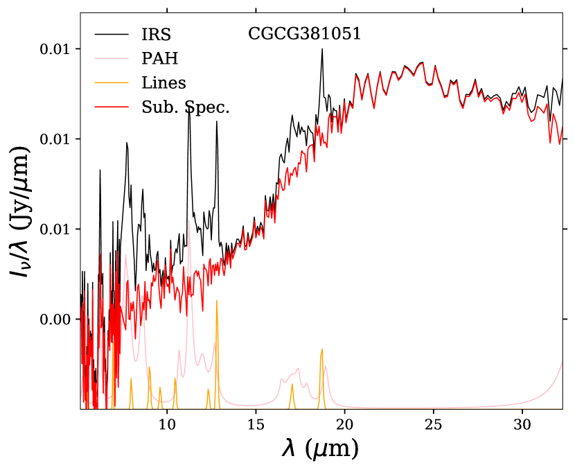
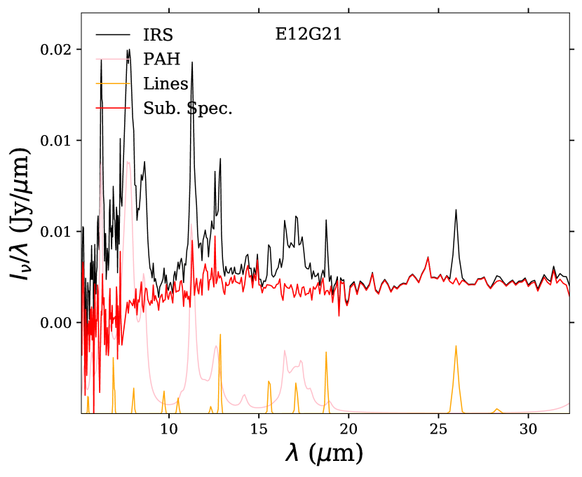
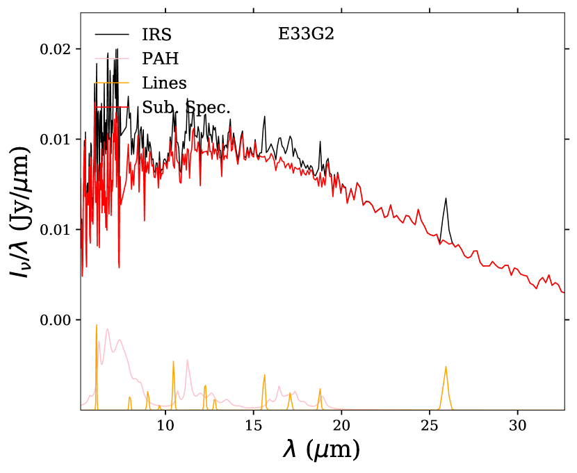
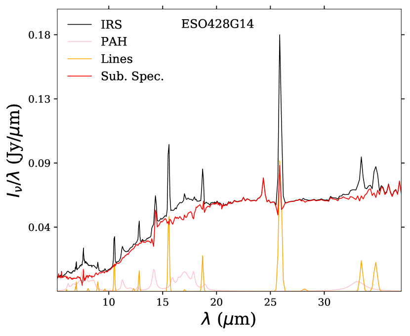
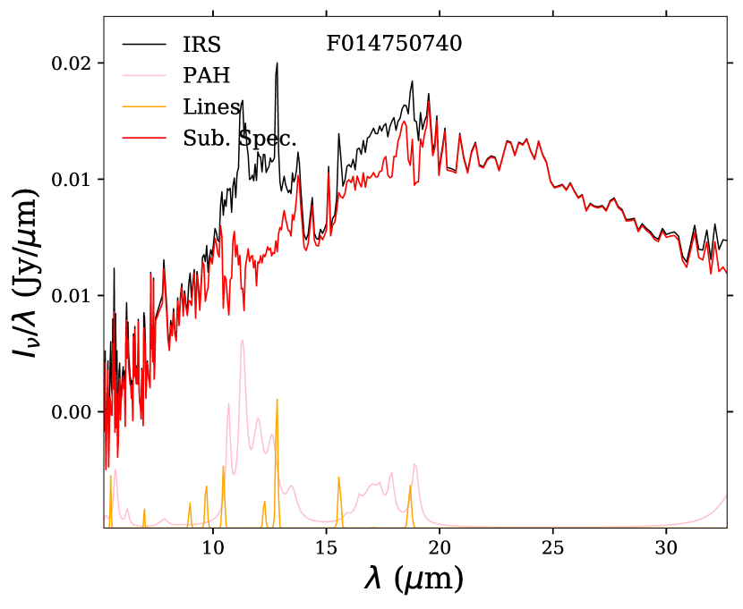
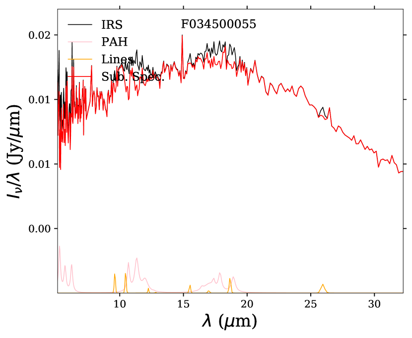
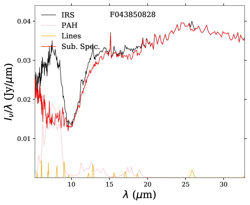
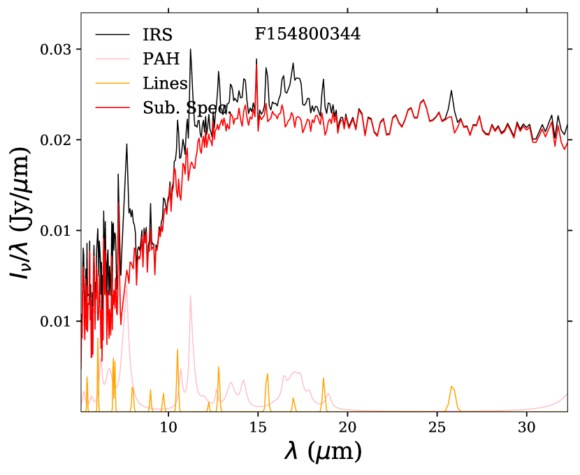
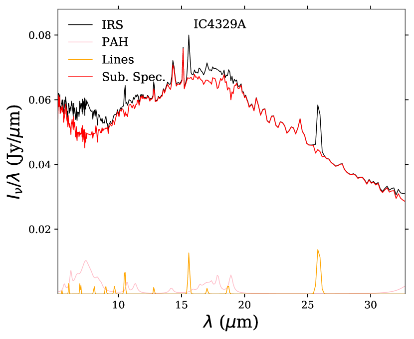
Figure B1: Individual spectral decomposition. We present the subtraction of the PAH and ionic lines emission from the spectra. The black lines represent the observed IRS spectra, while the orange and pink lines show the resulting adjust by fitting the PAH emission and ionic and hydrogen lines, respectively, using the pahfit (Smith et al., 2007b). In red are presented the subtracted spectra that were adopted in our analysis.

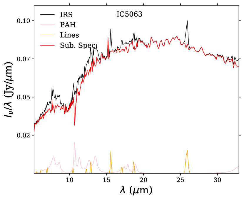
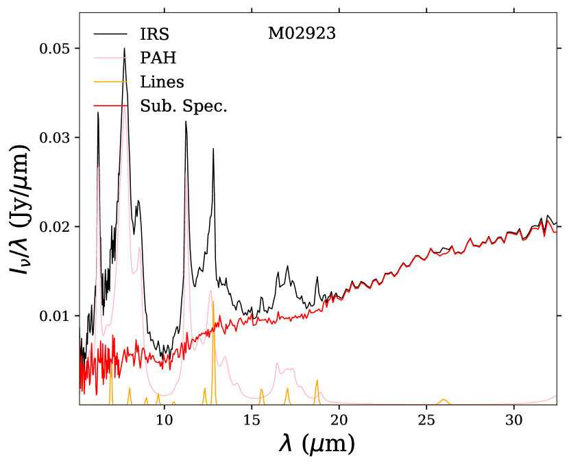
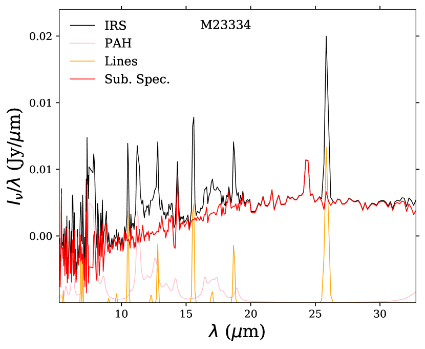
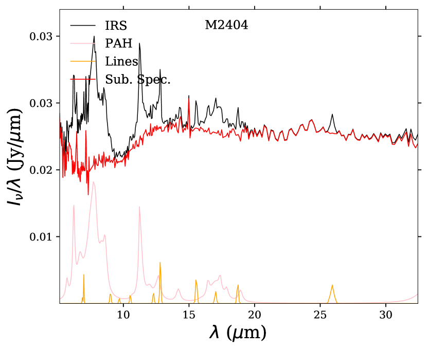
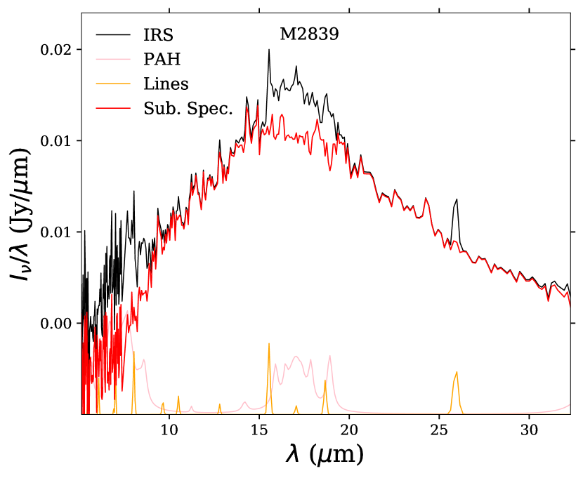
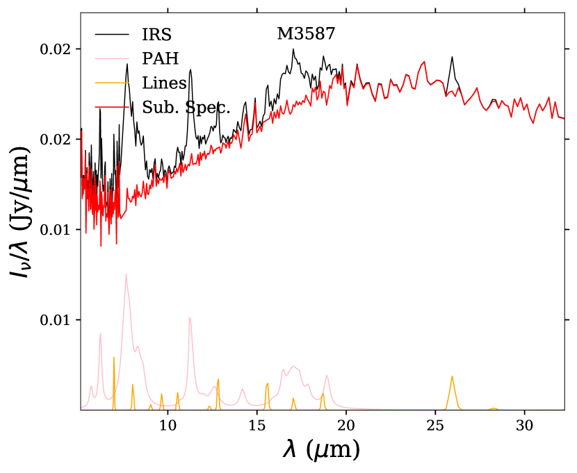
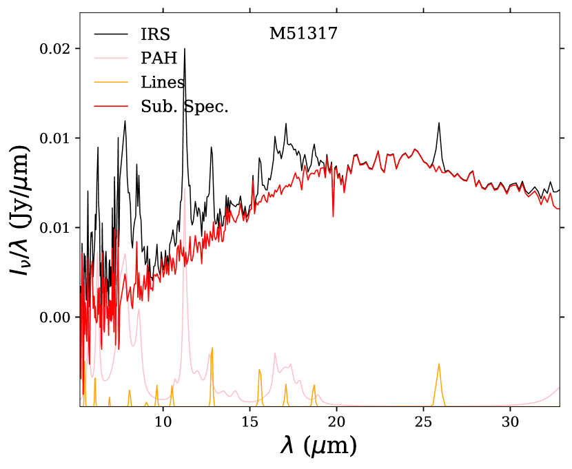
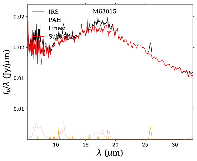
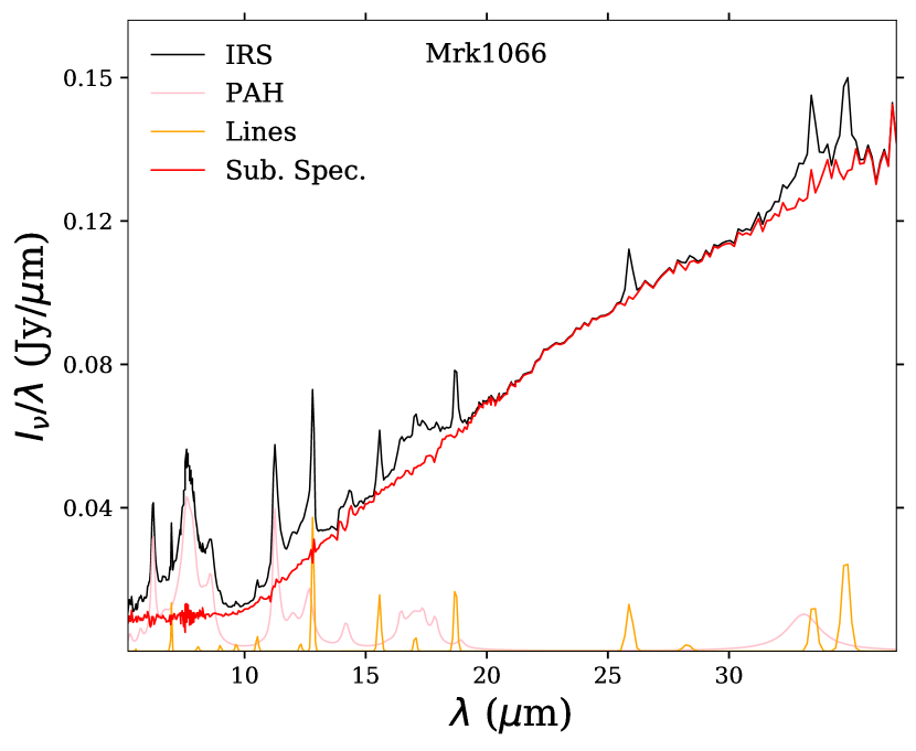
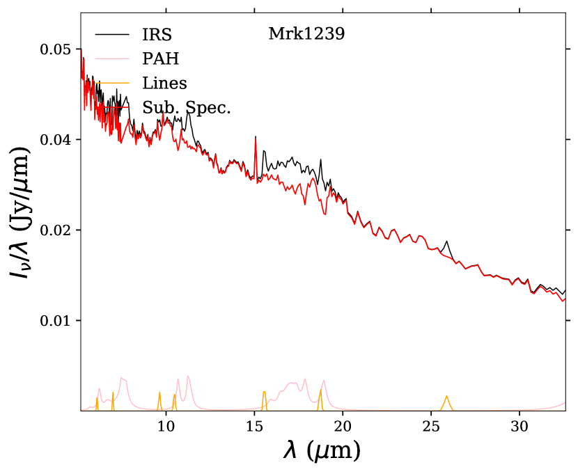
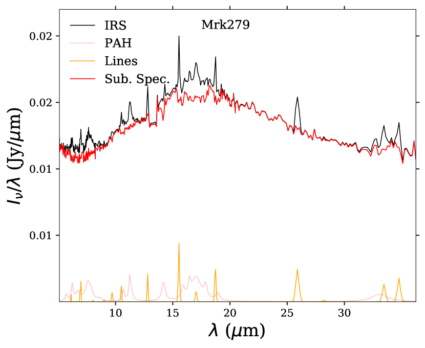
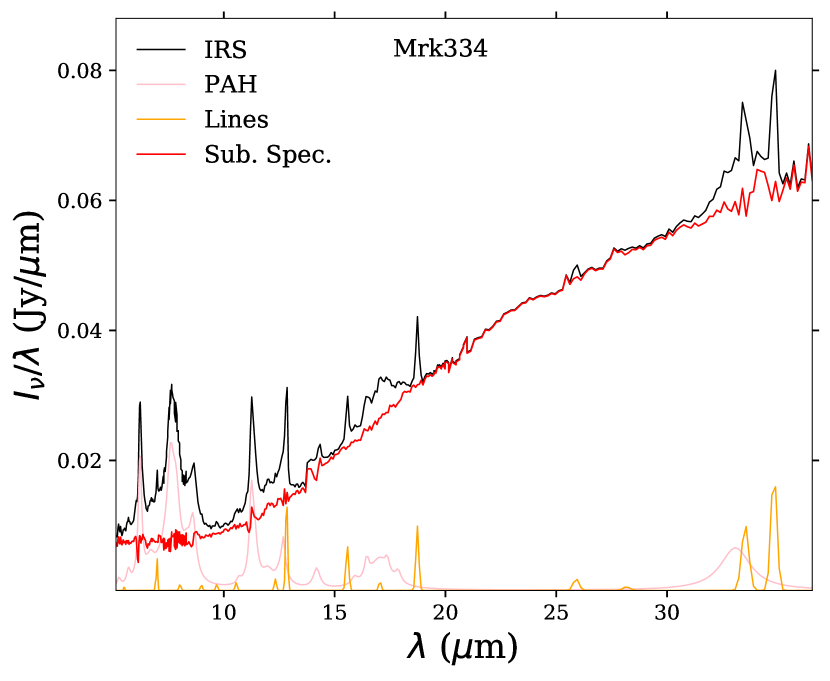
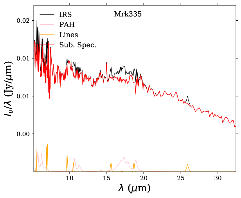
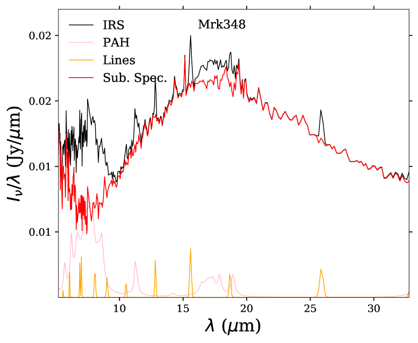
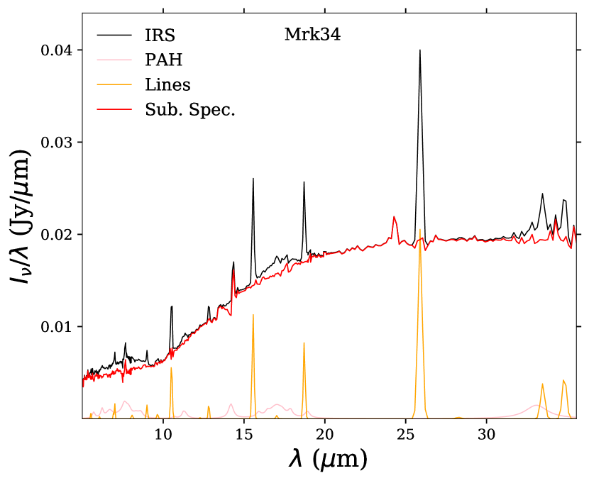
Figure B1: continued from previous page.

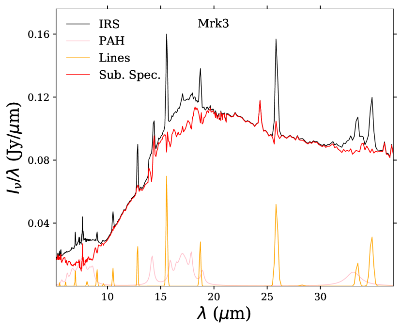
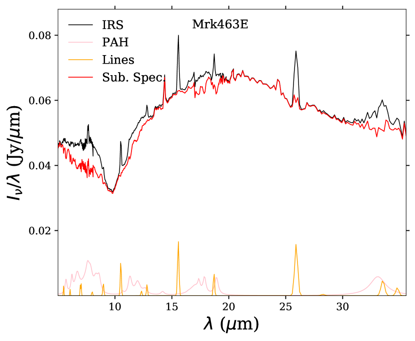
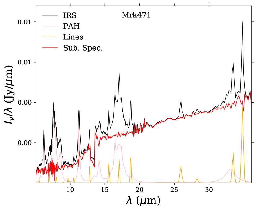
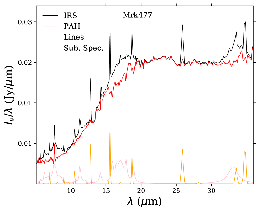
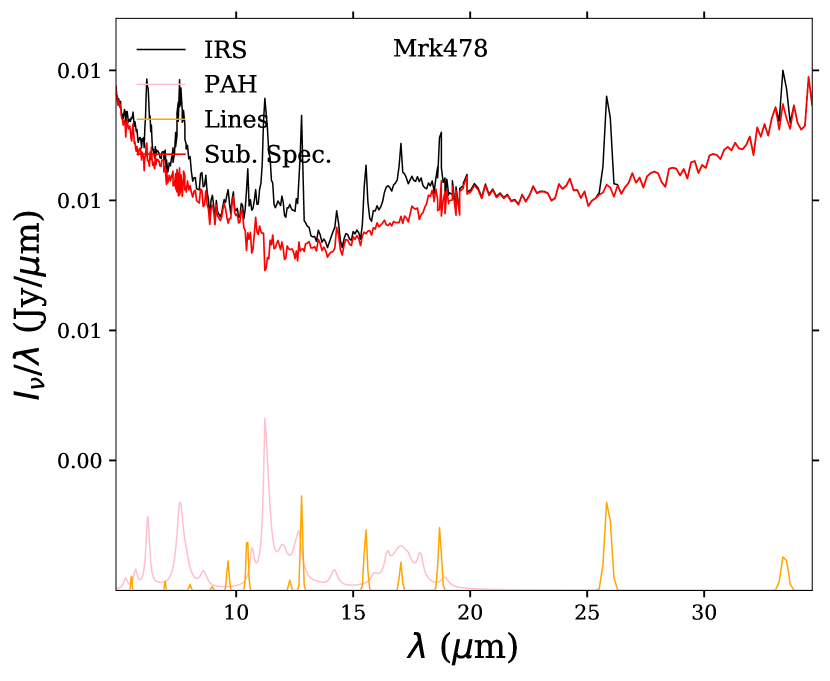
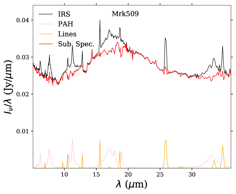
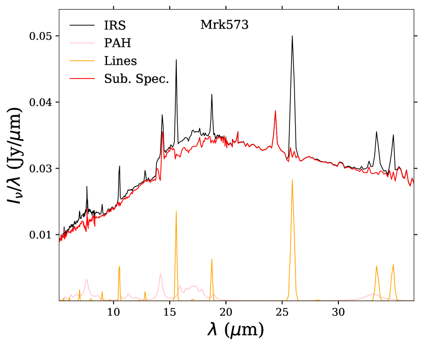
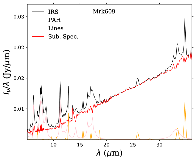
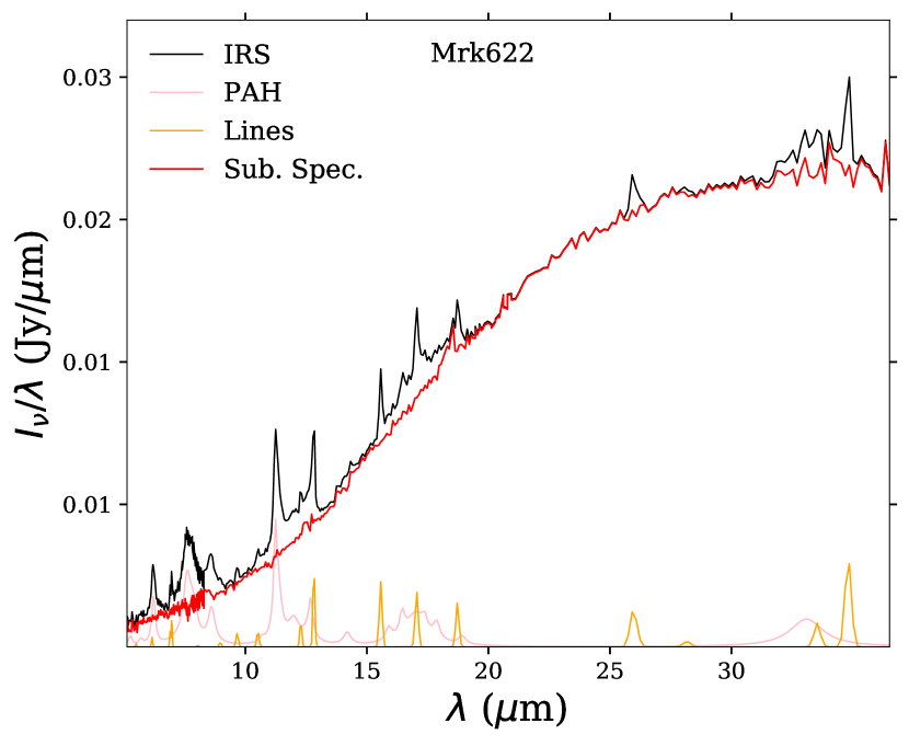
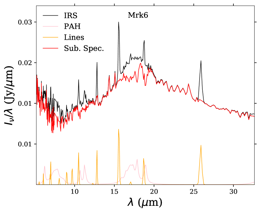
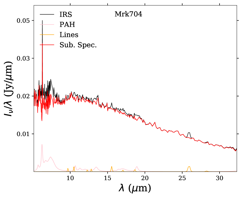
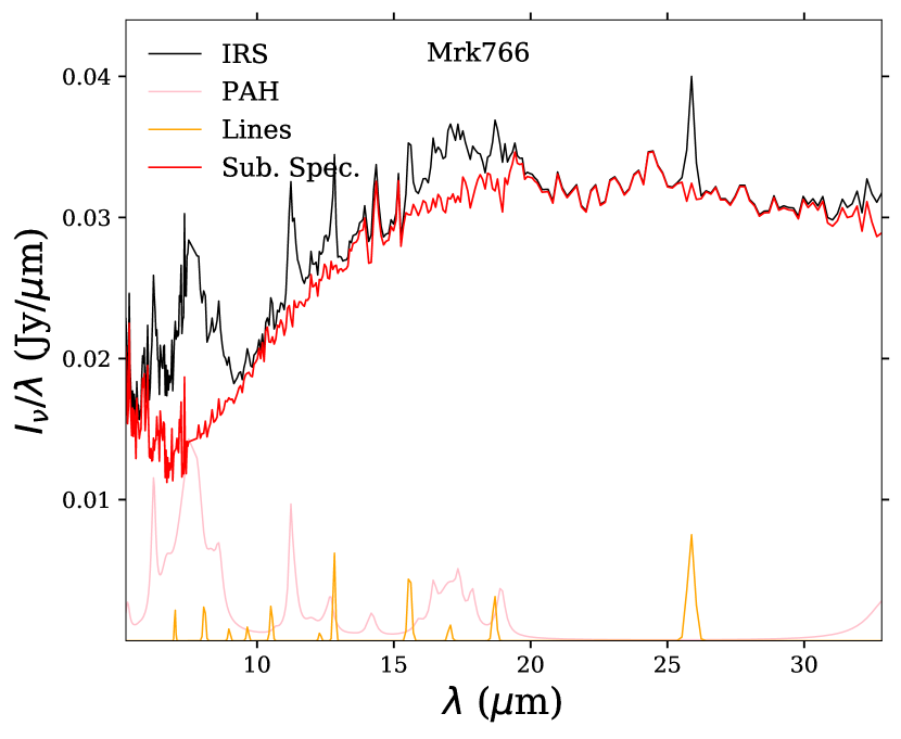
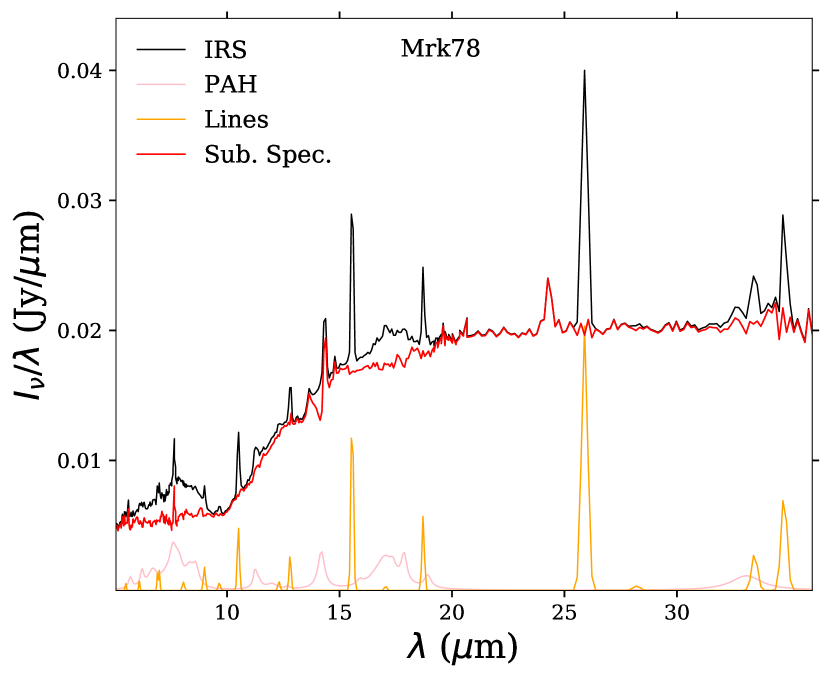
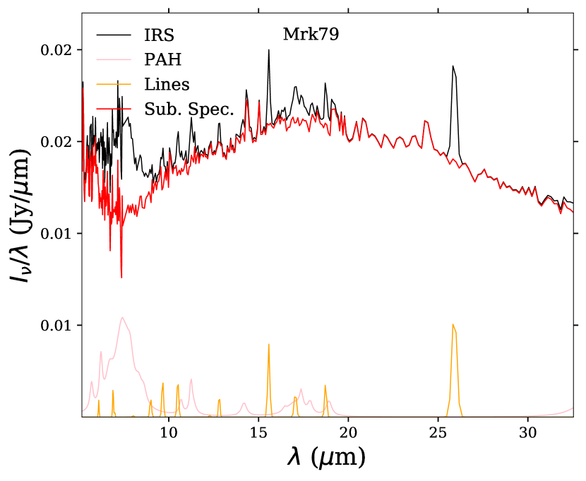
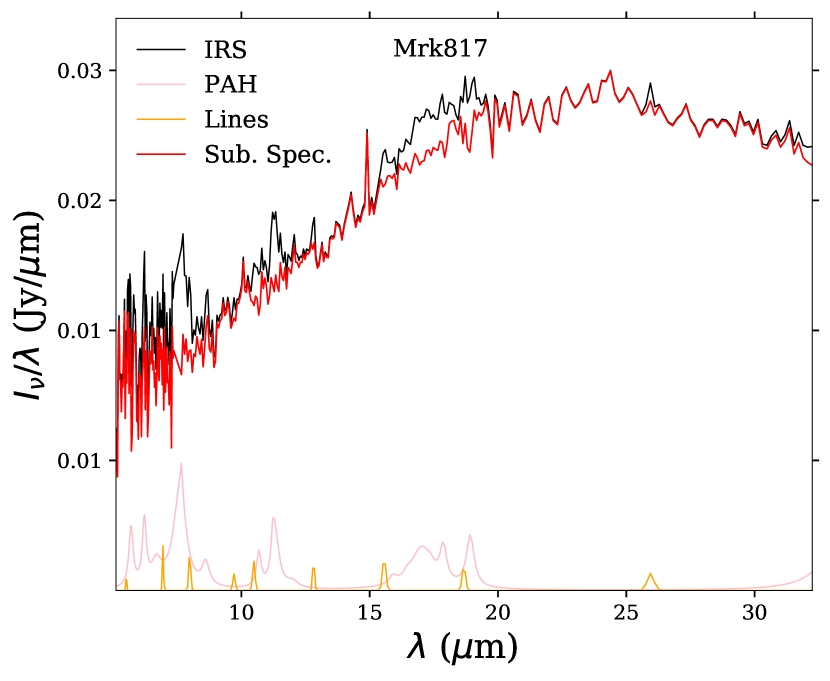
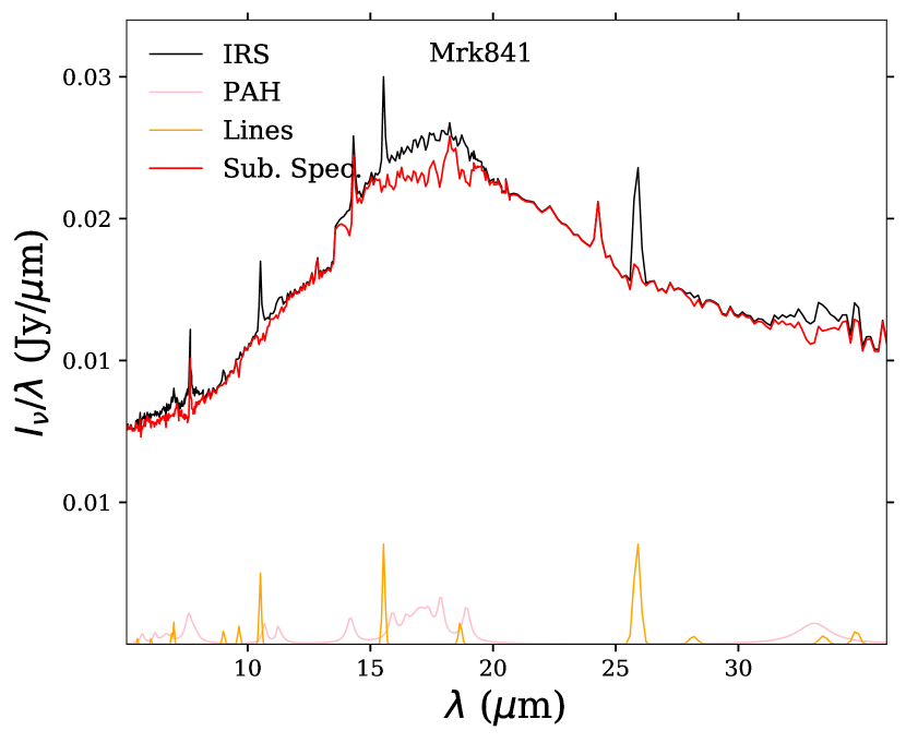
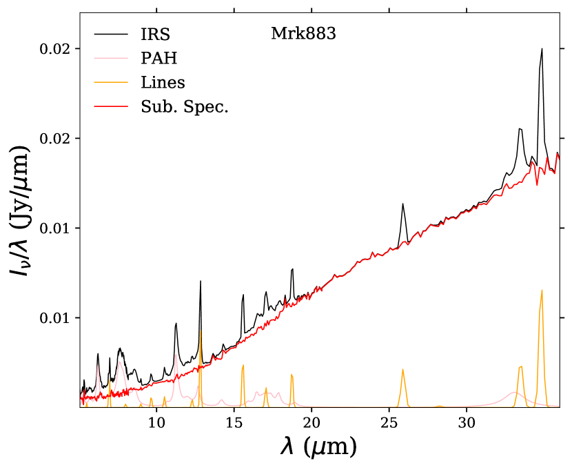
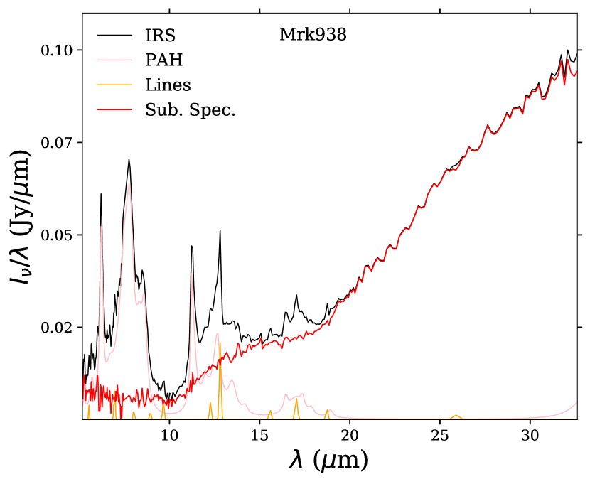
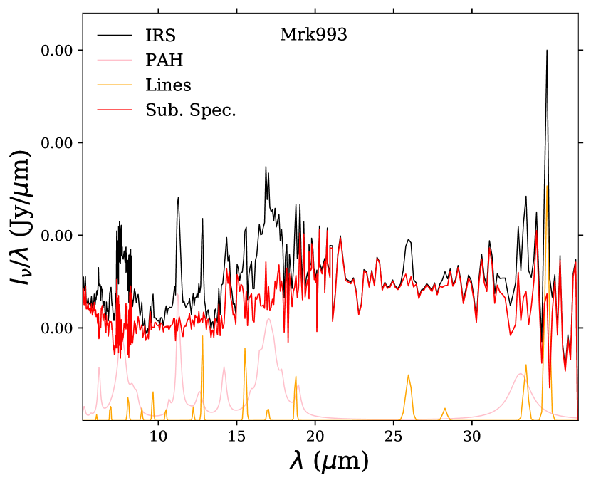
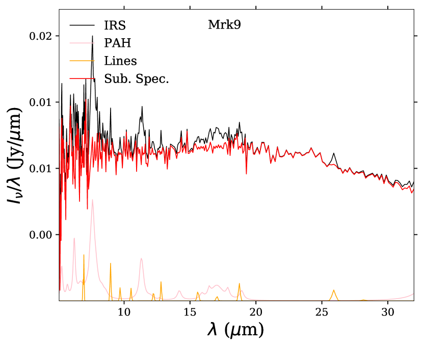
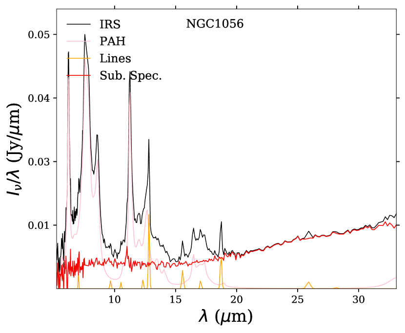
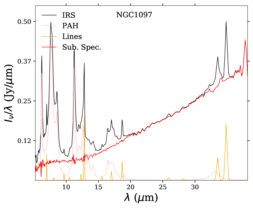
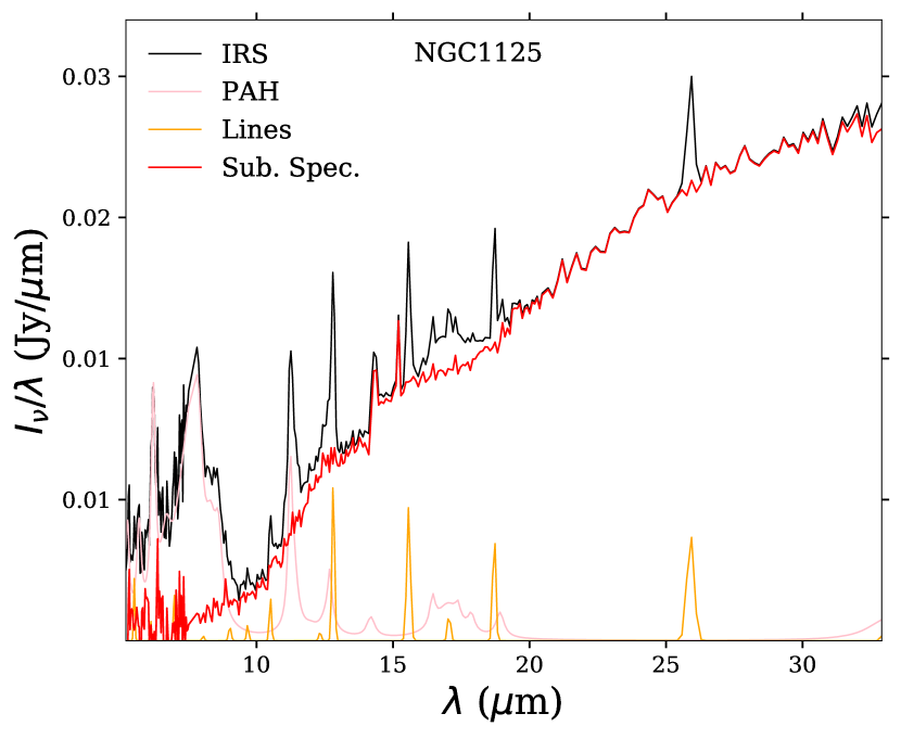
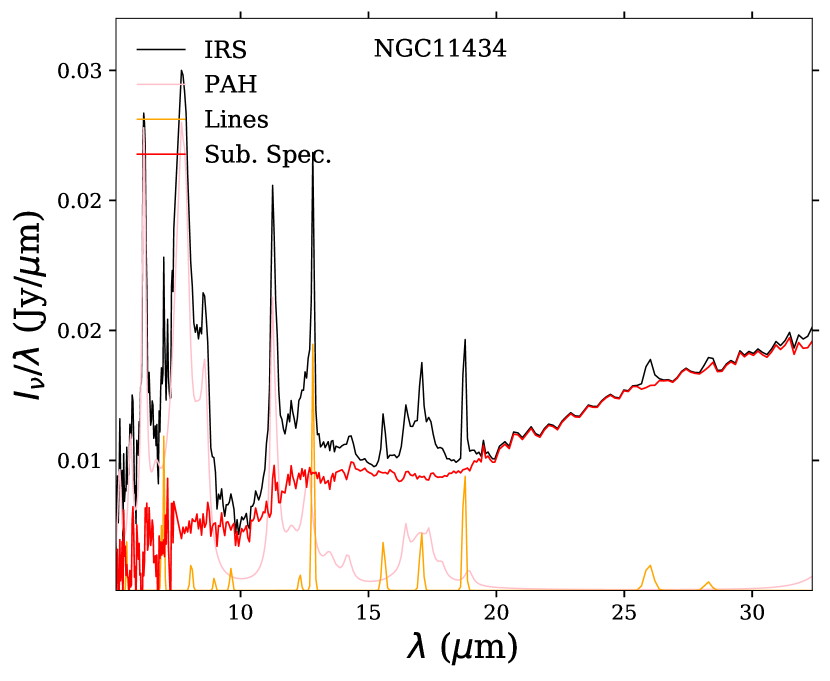
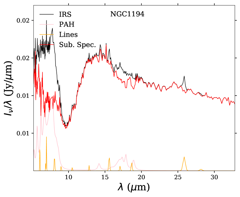
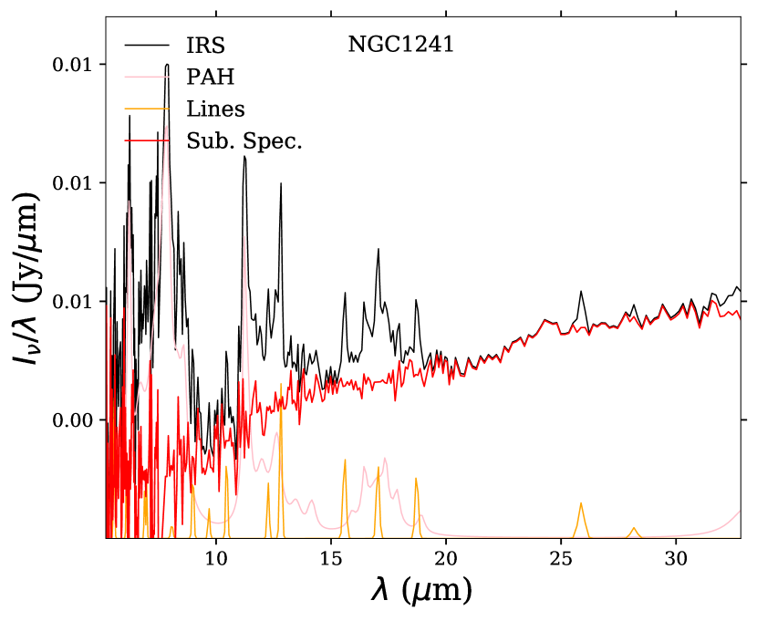
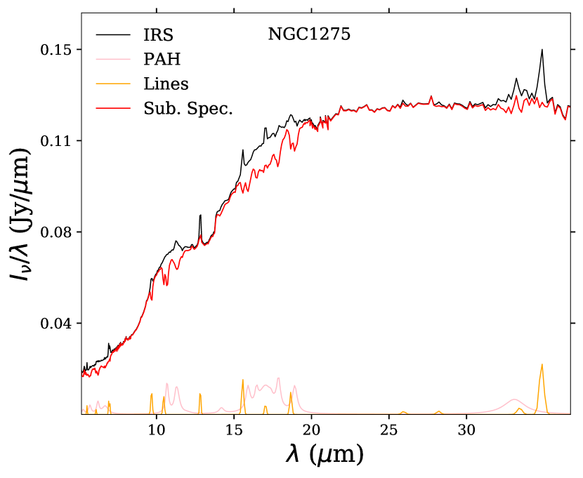
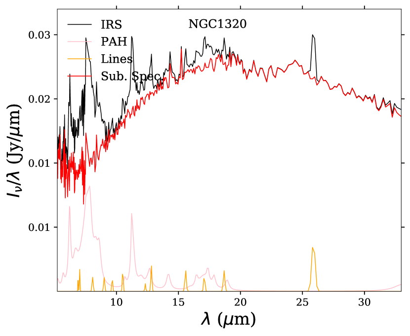
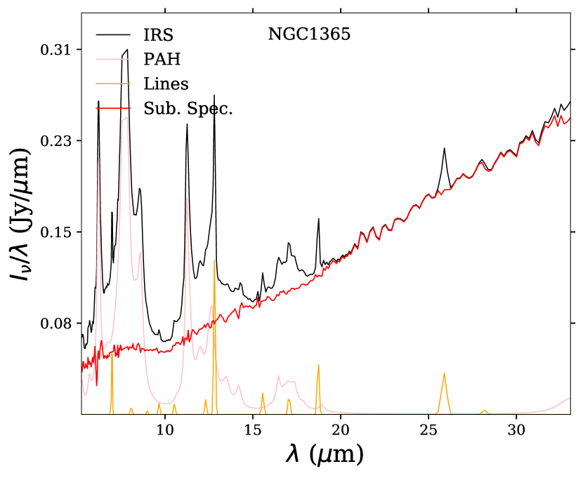
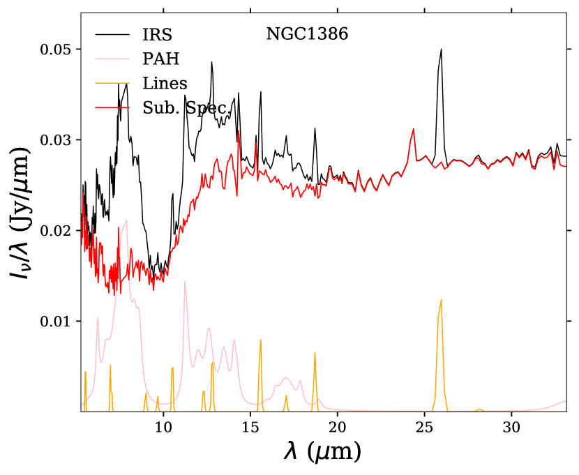
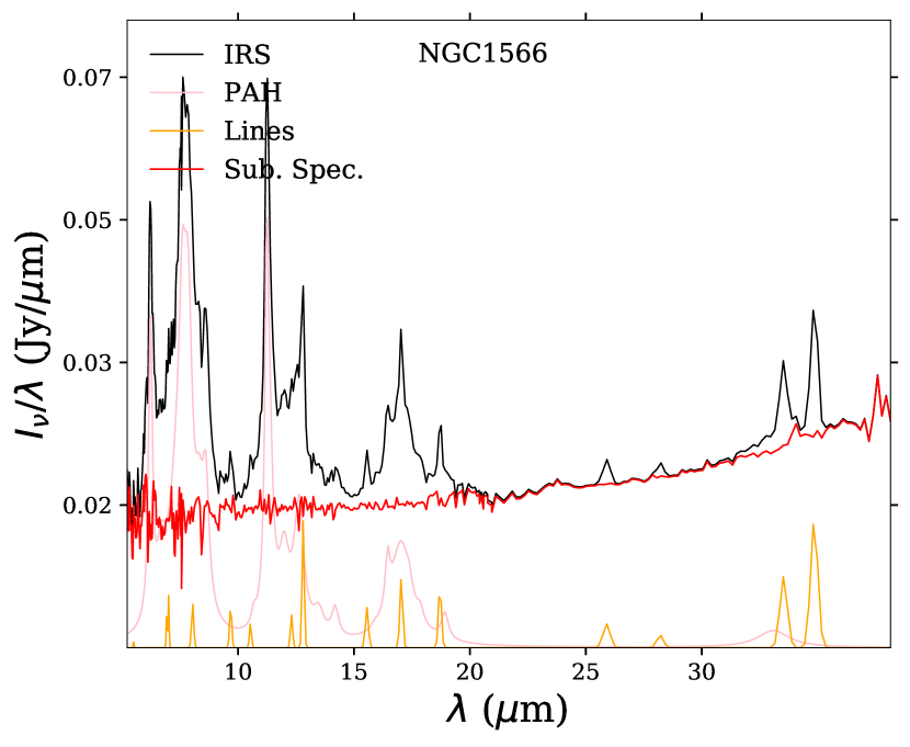
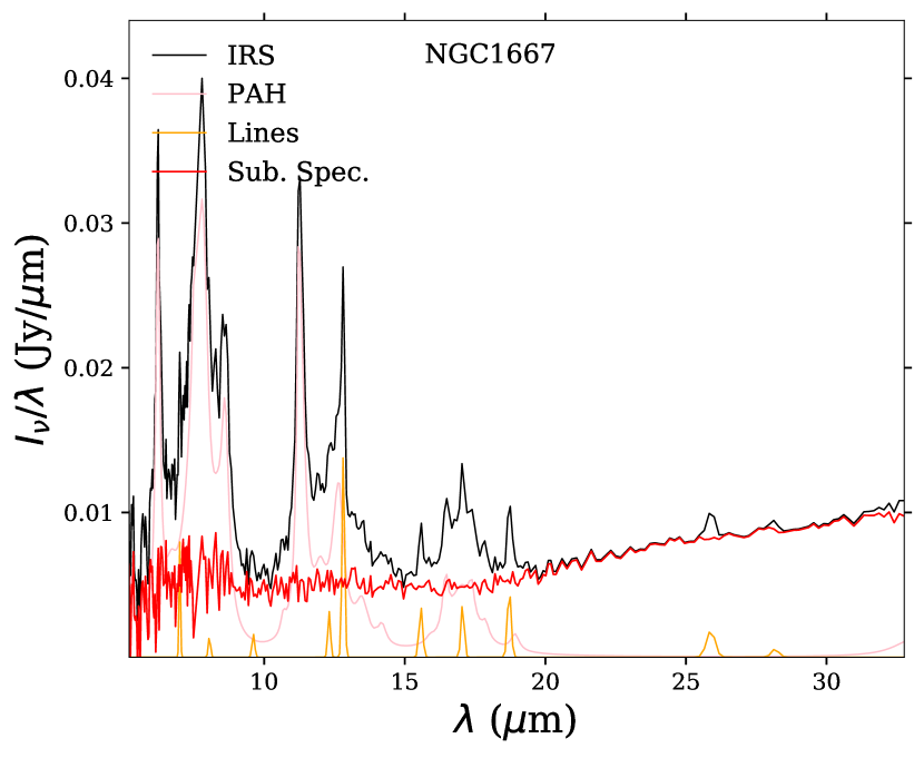
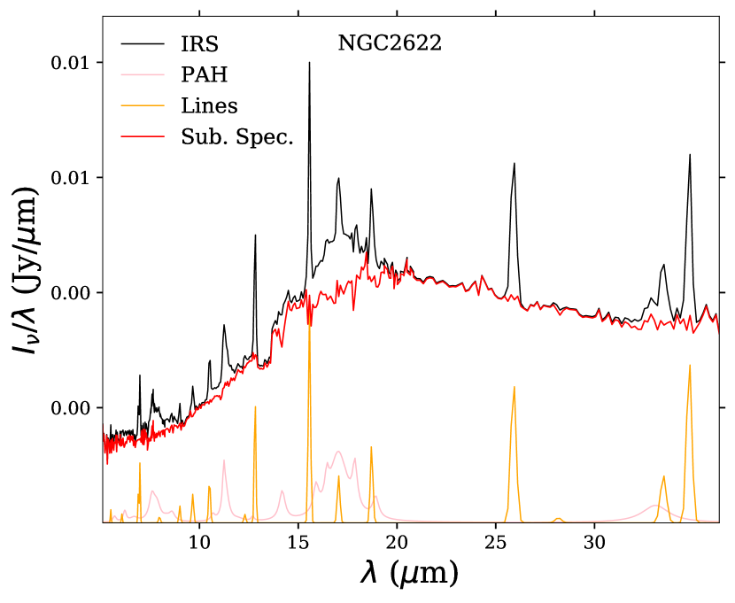
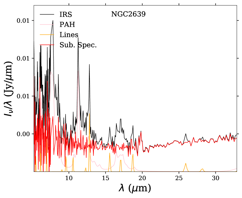
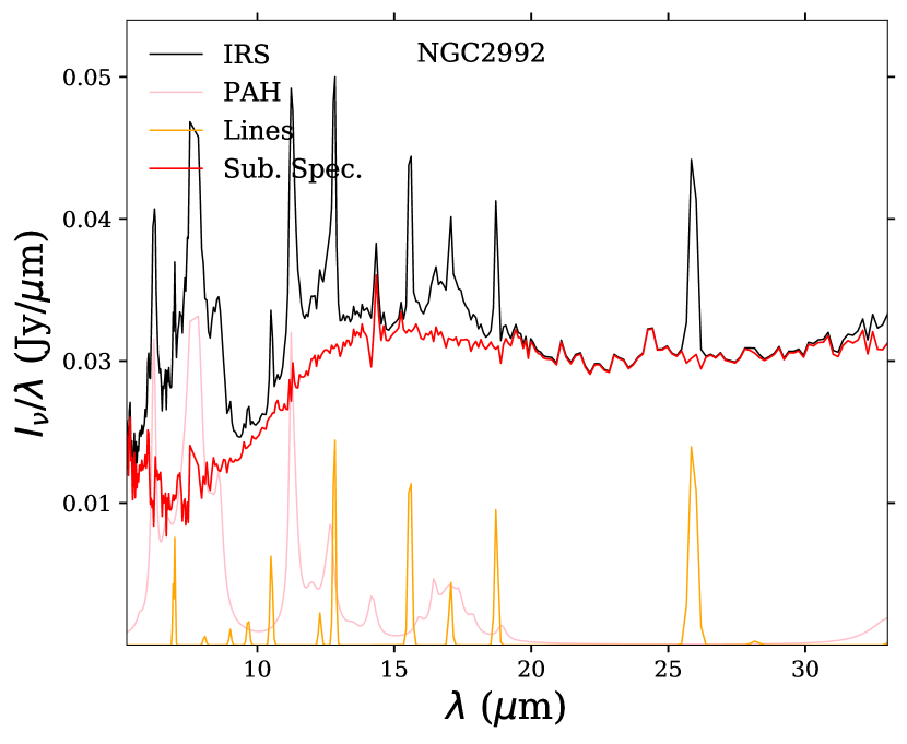
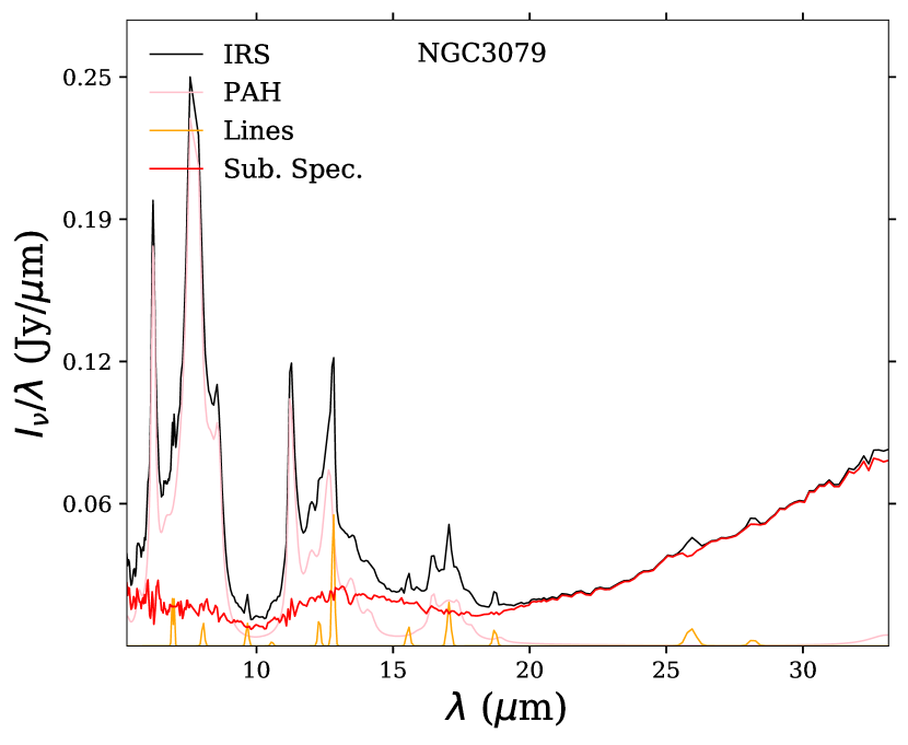
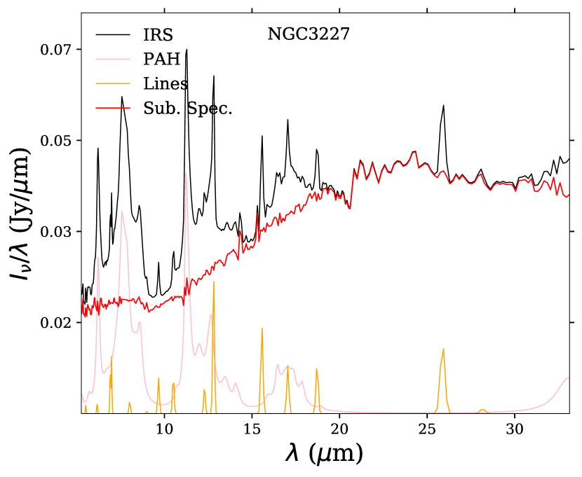
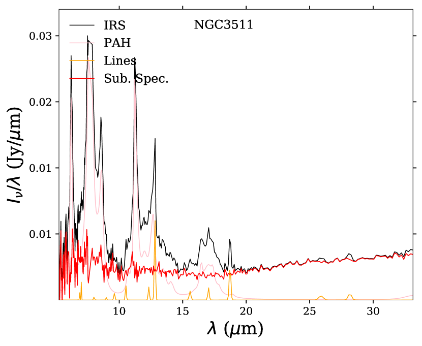
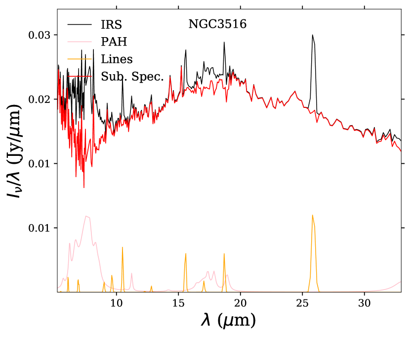
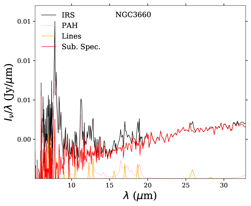
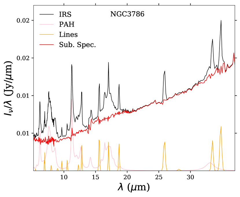
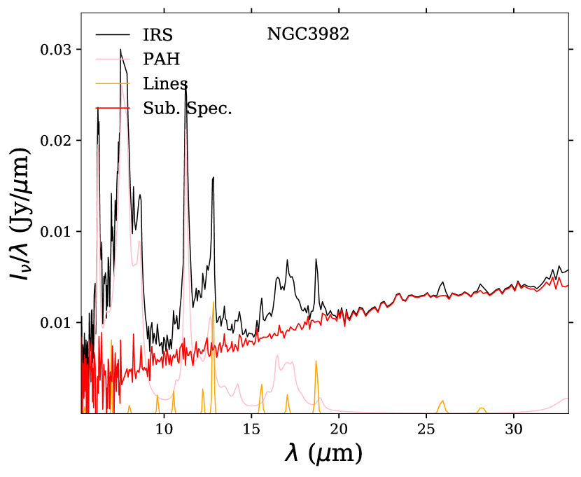
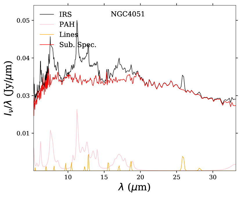
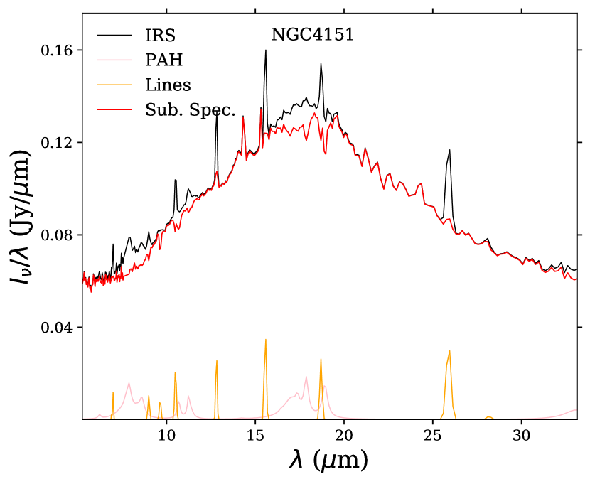
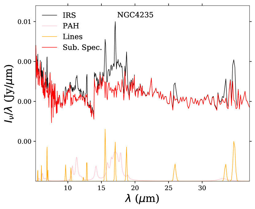
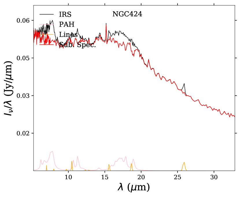
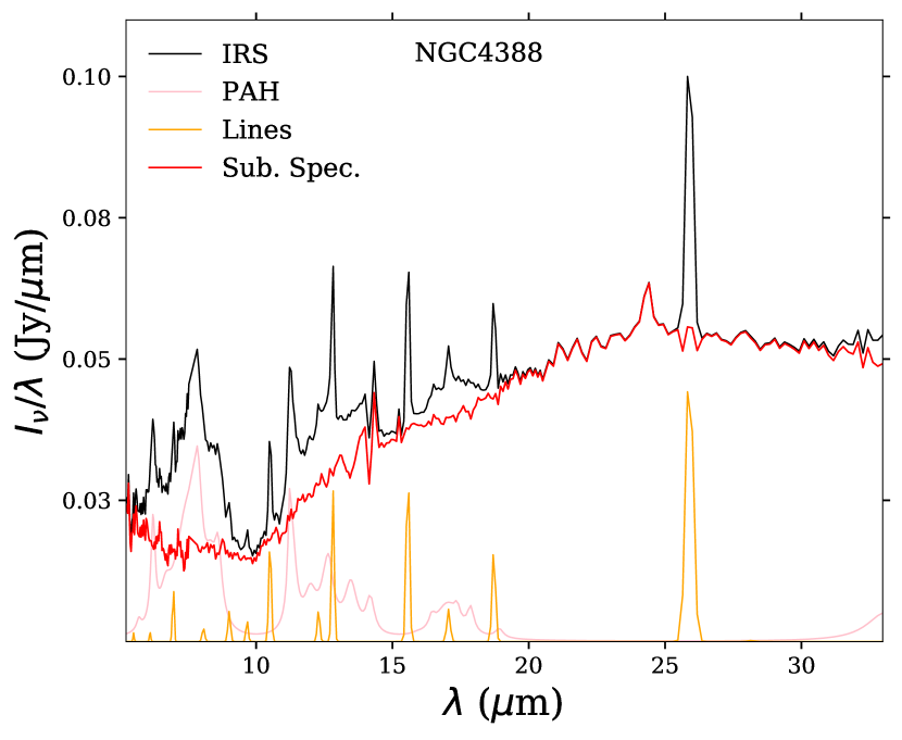
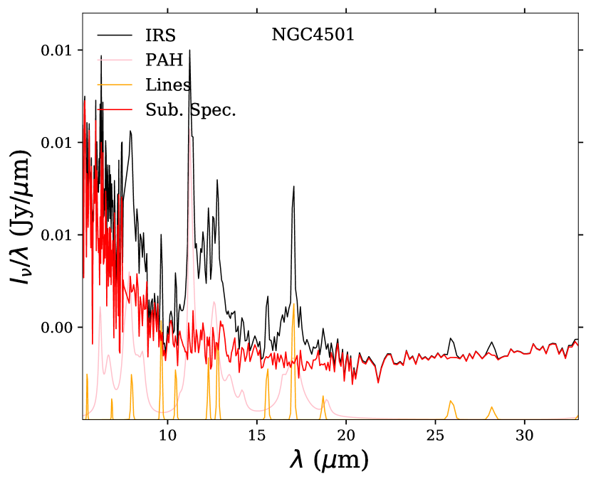
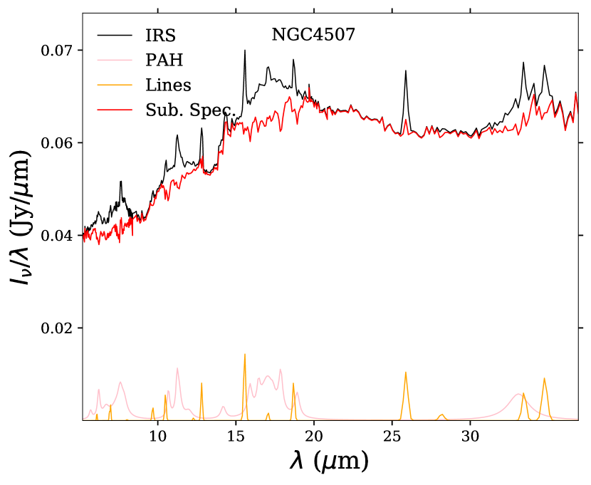
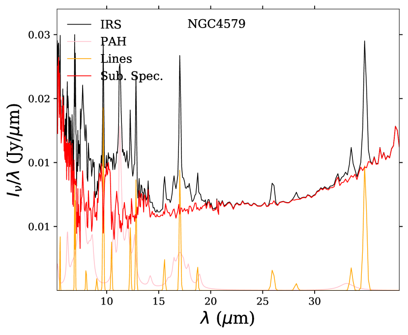
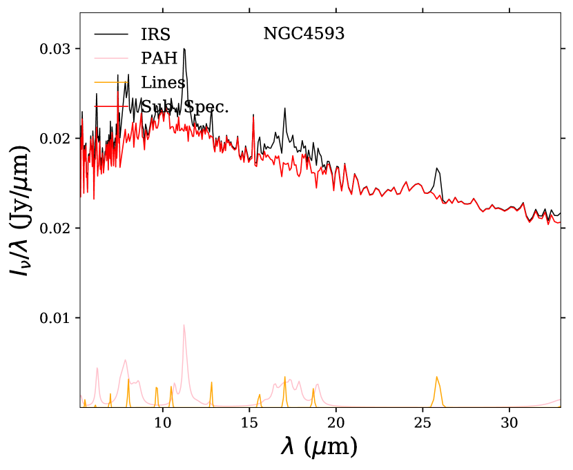
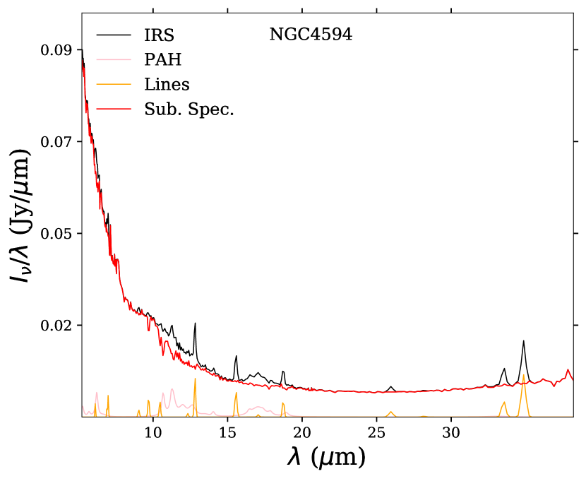
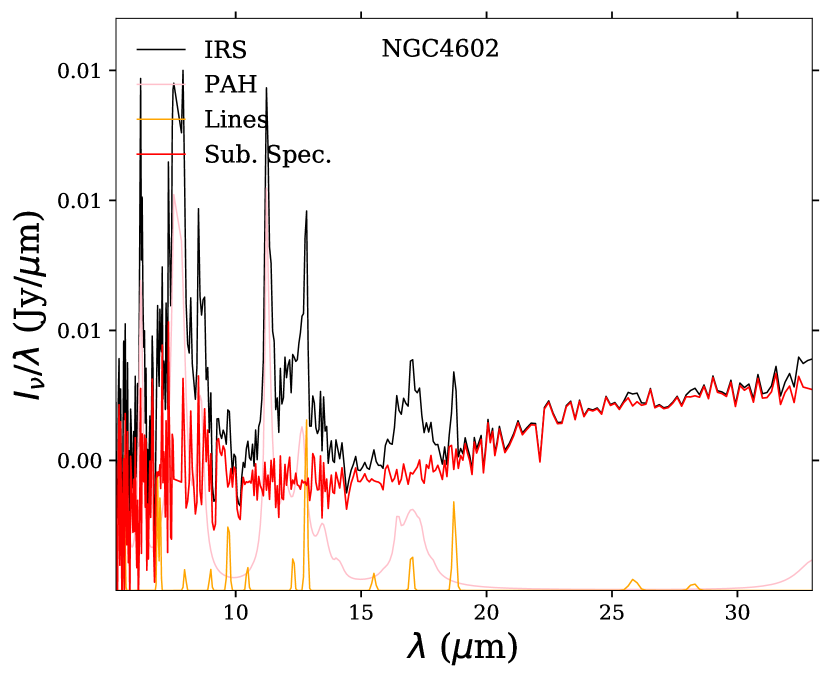
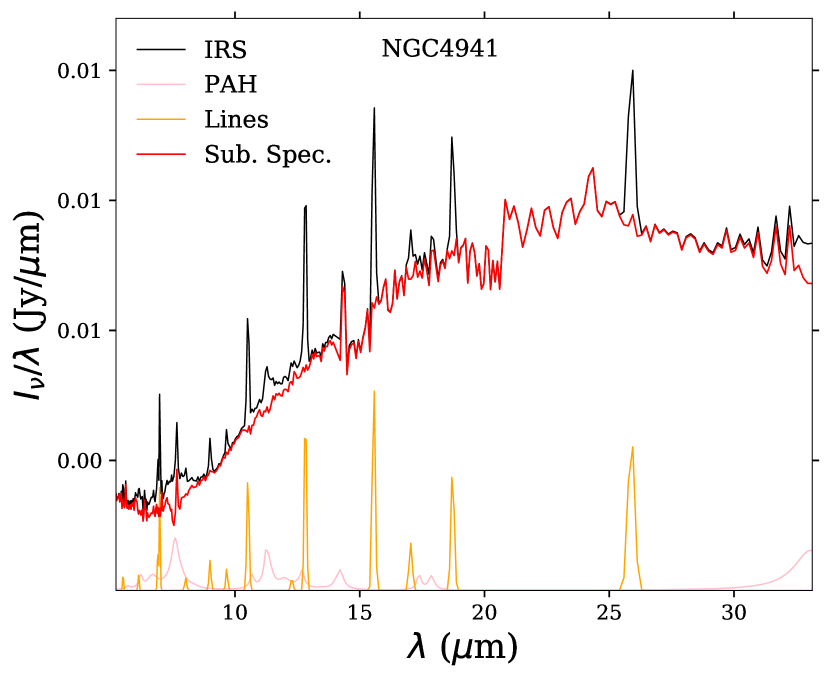
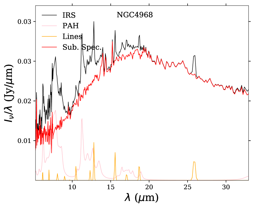
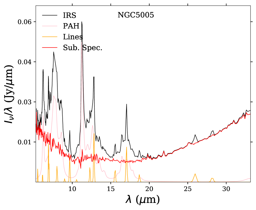
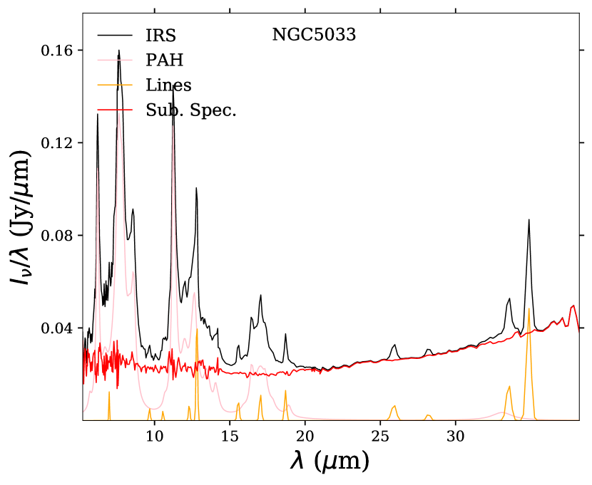
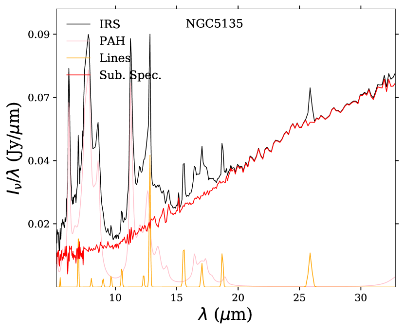
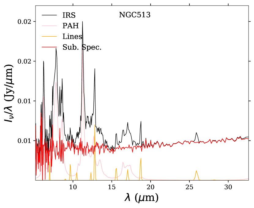
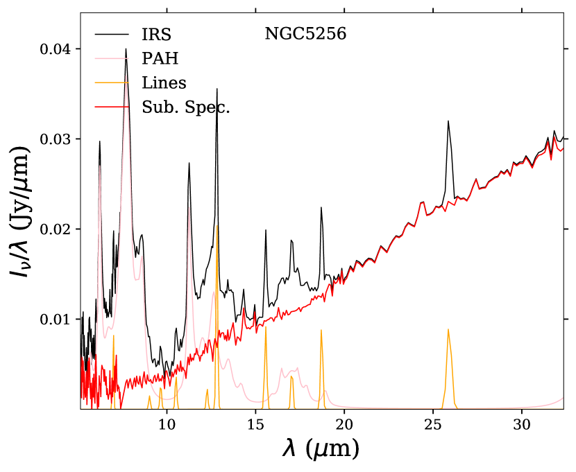
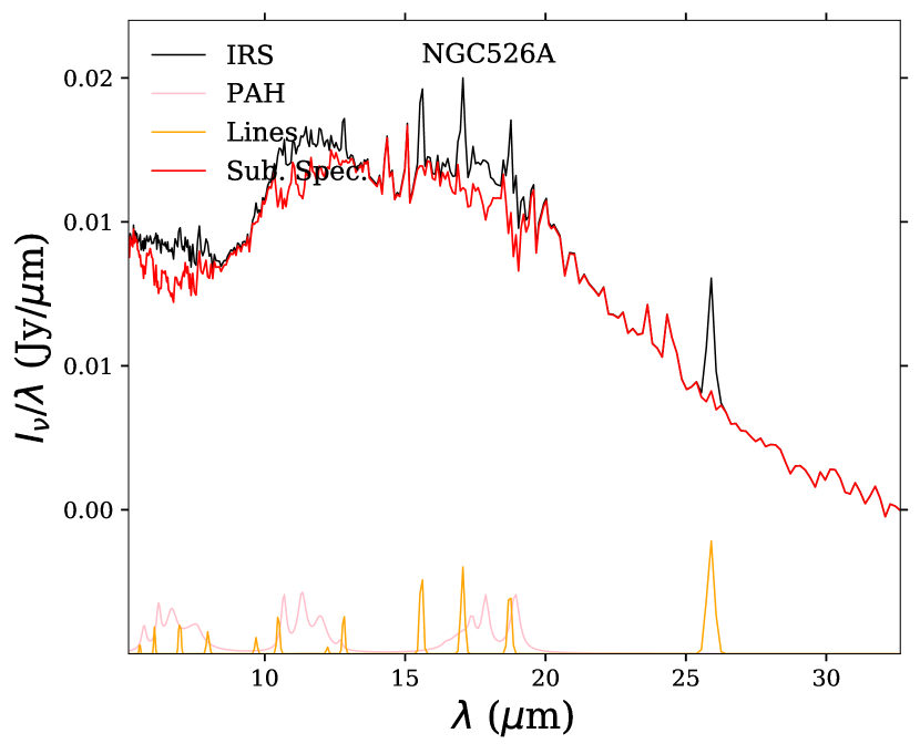
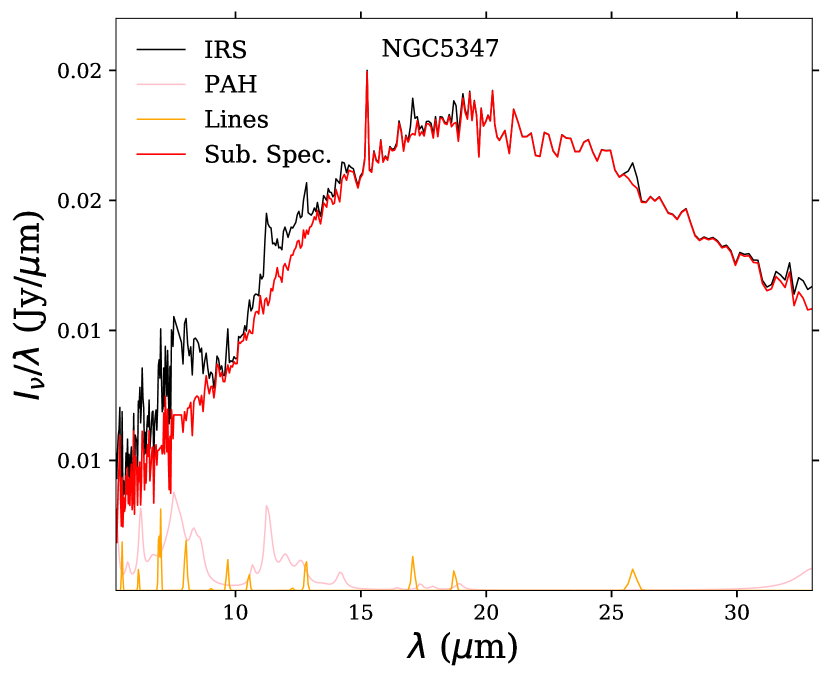
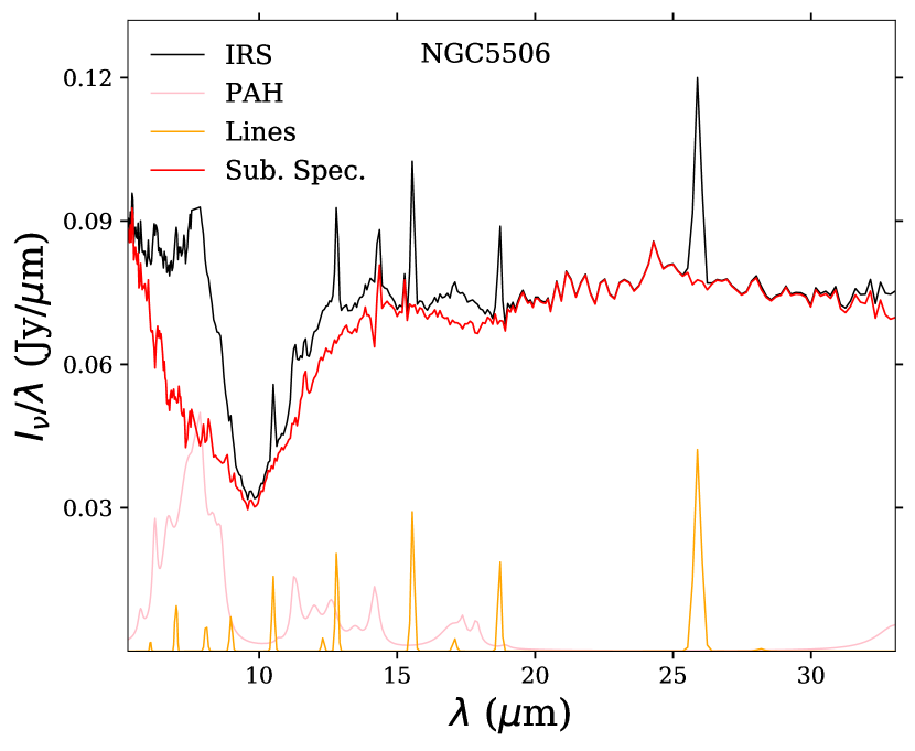
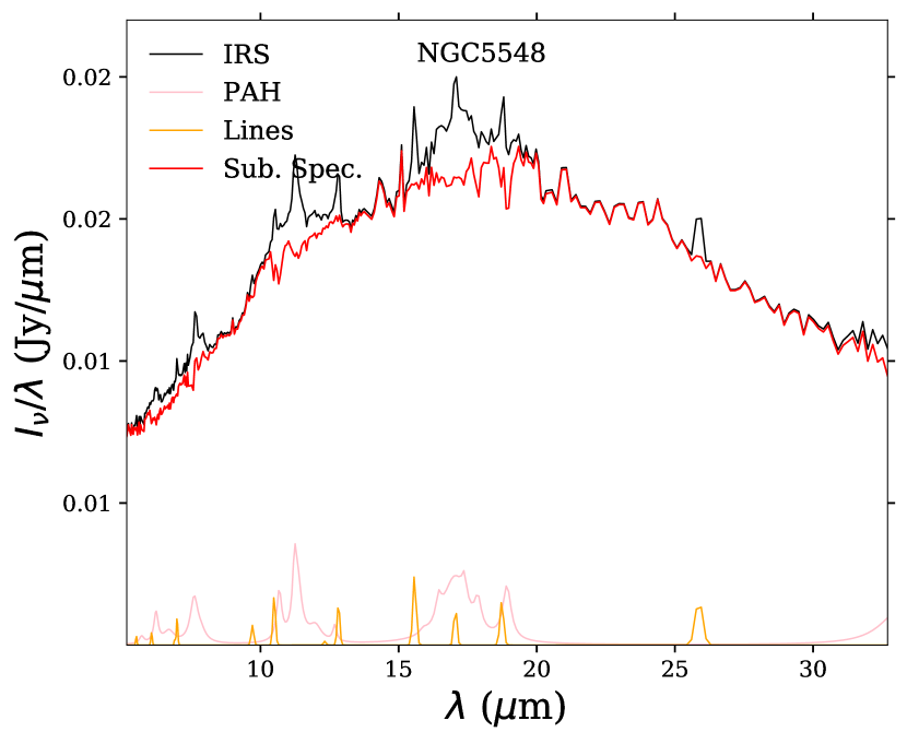
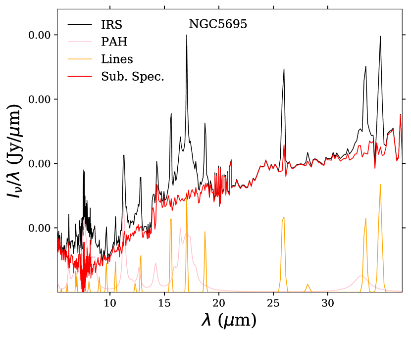
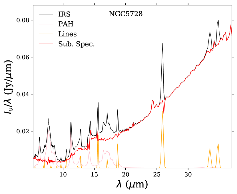
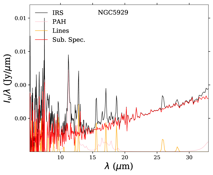
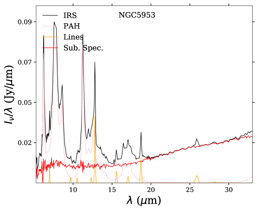
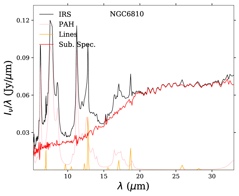
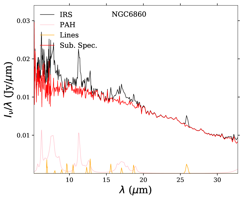
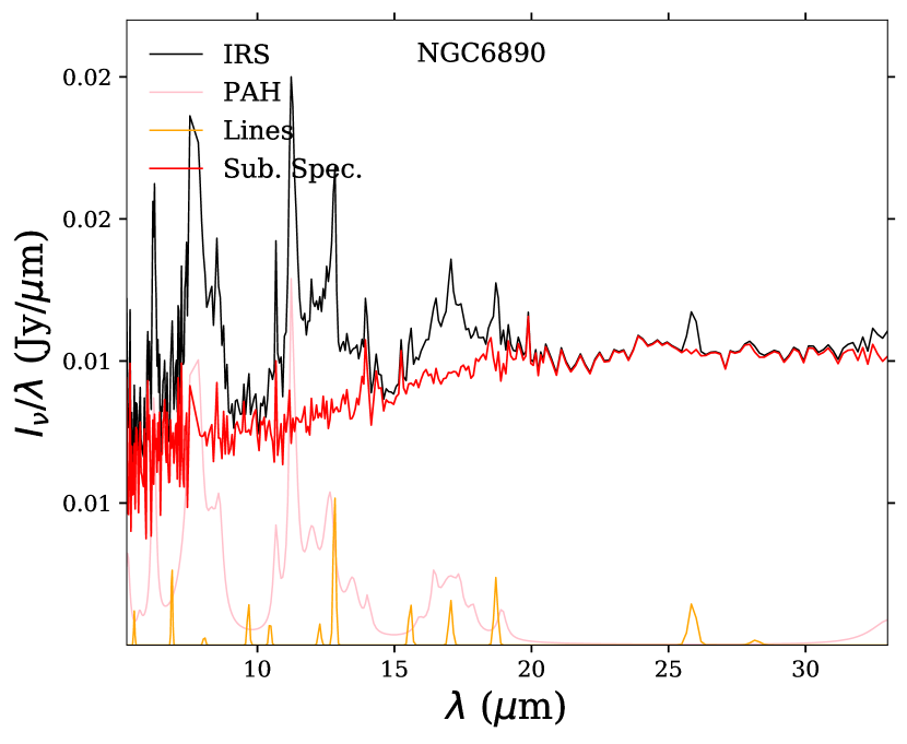
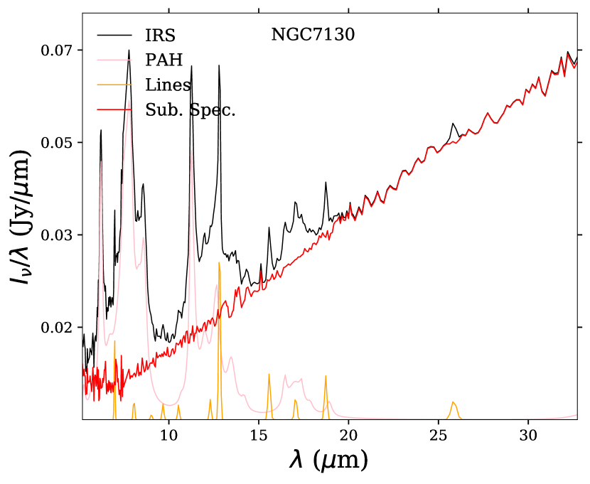
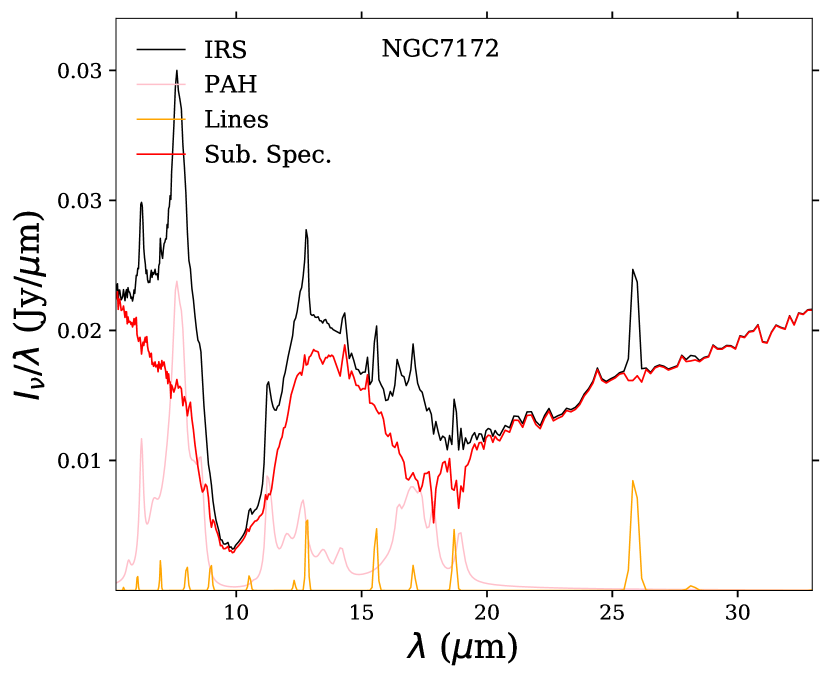
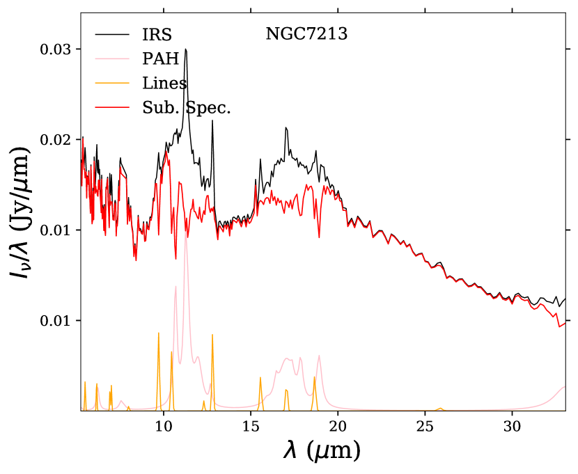
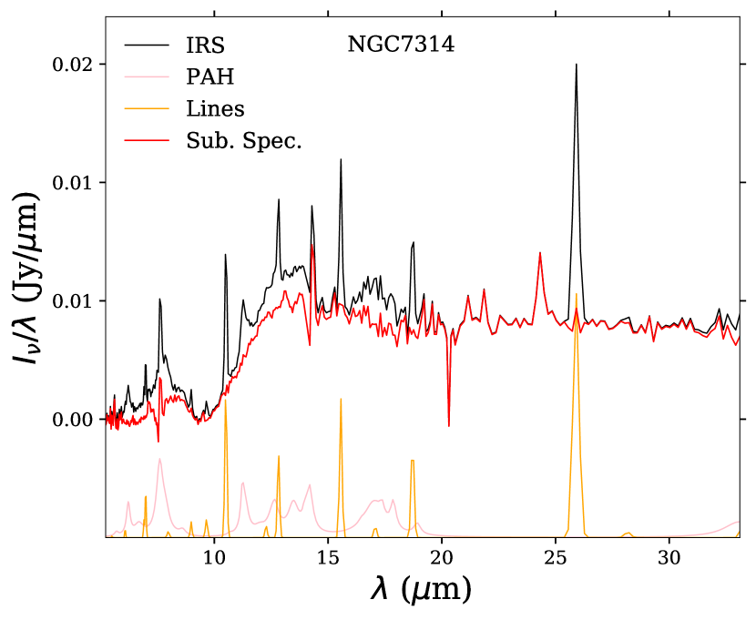
Figure B1: continued from previous page.

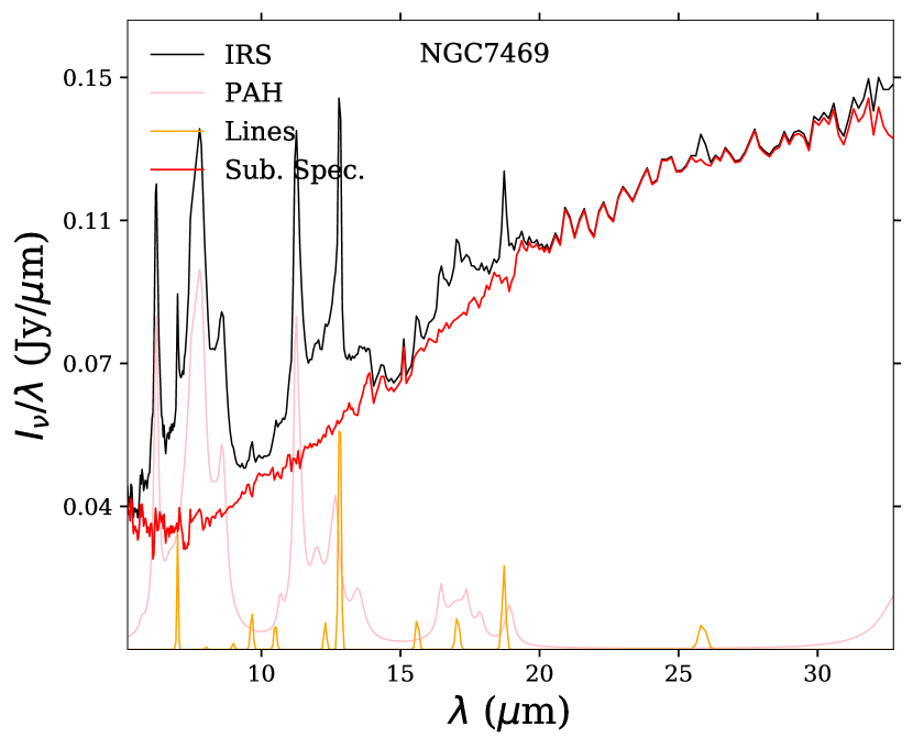
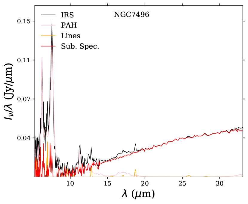
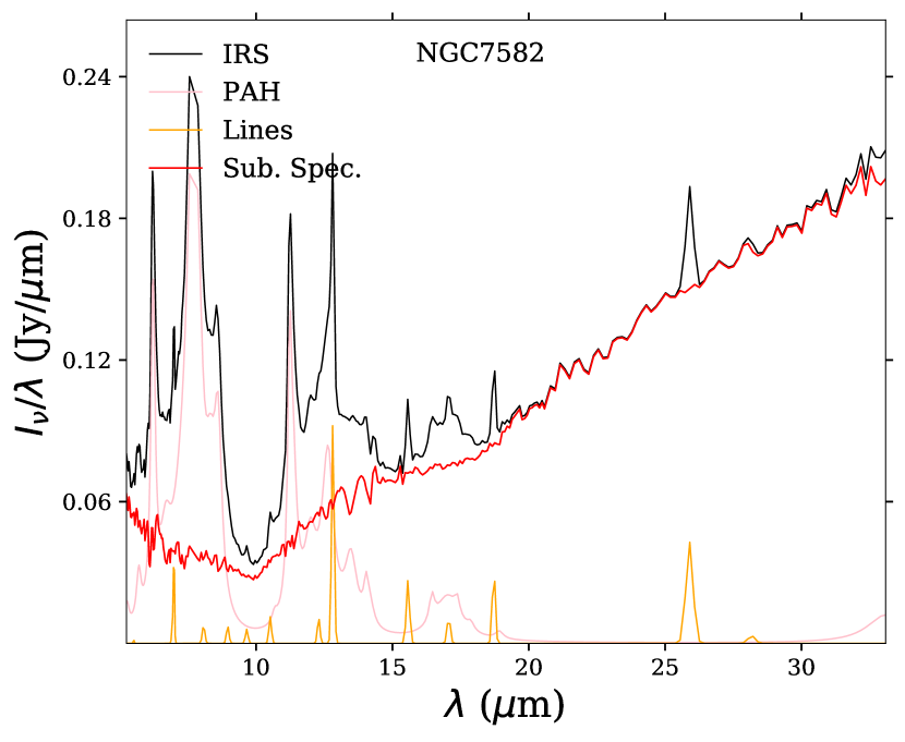
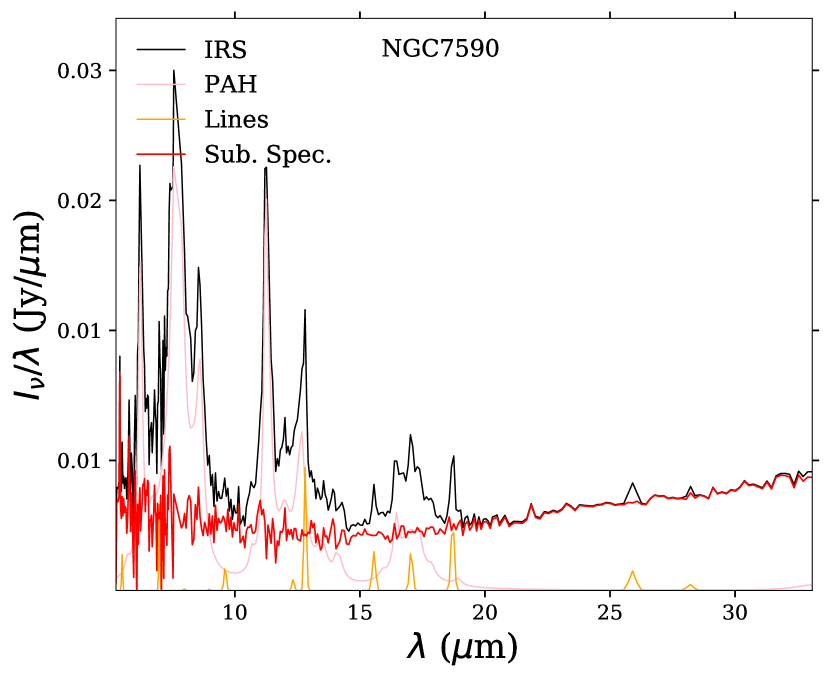
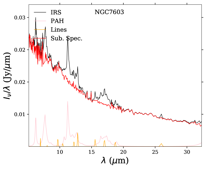
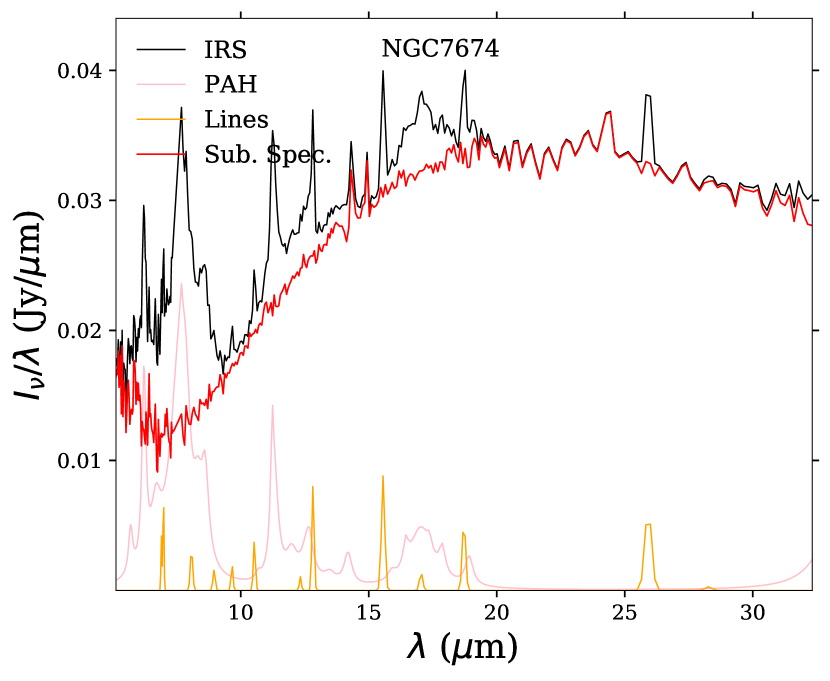
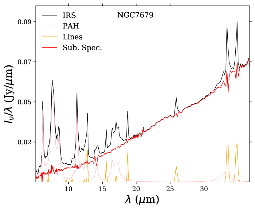
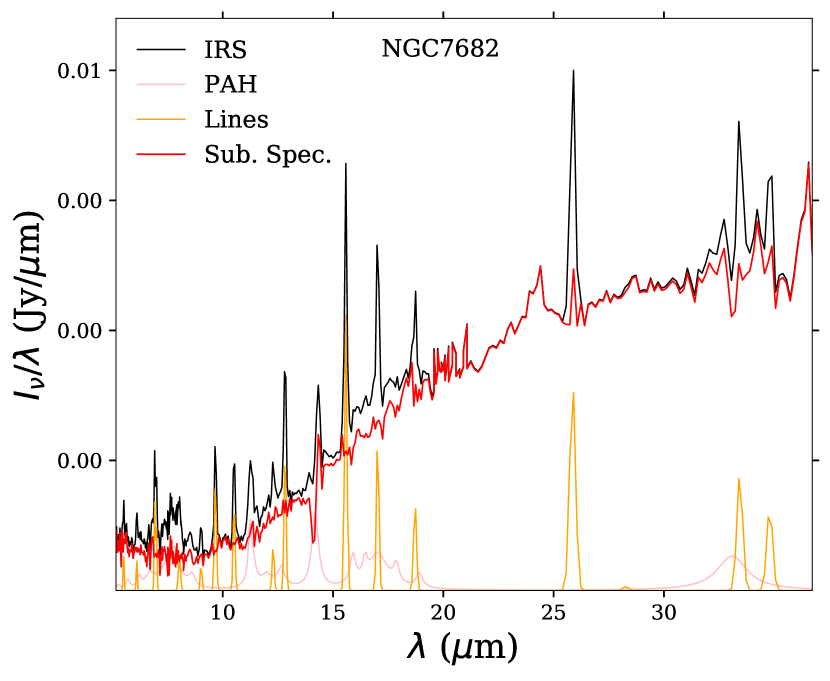
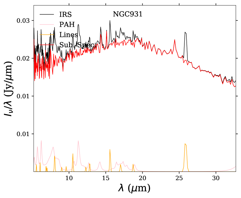
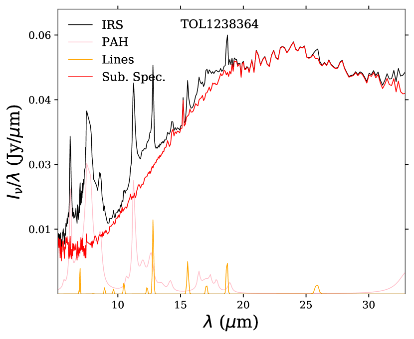
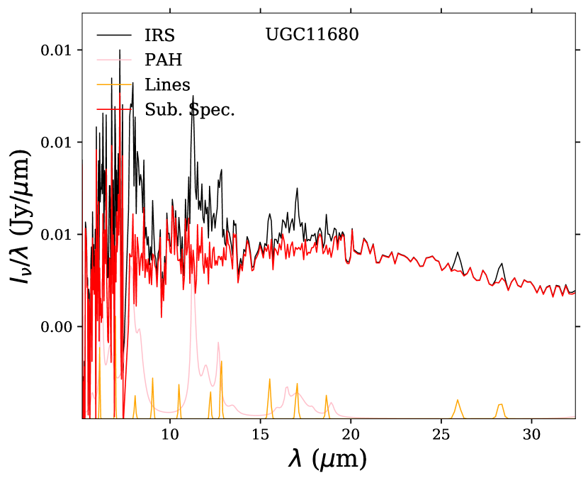
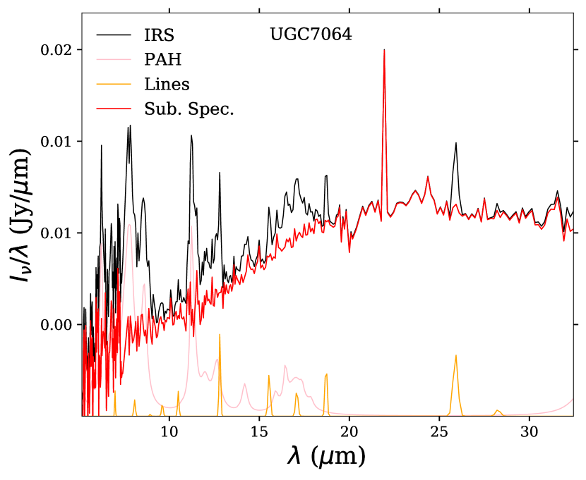
Figure B1: continued from previous page.

Figure B1: continued from previous page.

Figure B1: continued from previous page.

Figure B1: continued from previous page.

Figure B1: continued from previous page.

Appendix C Individual Adjusts

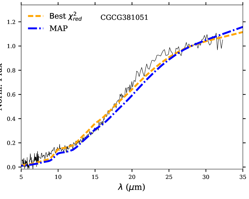
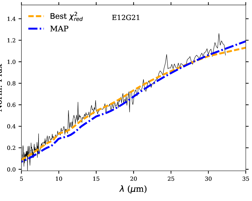
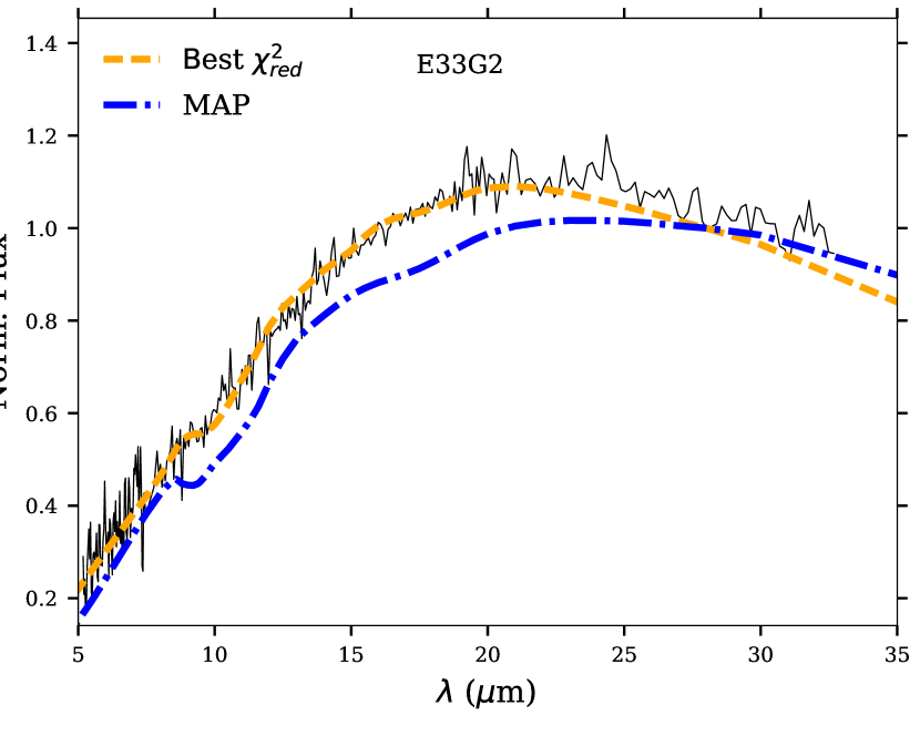
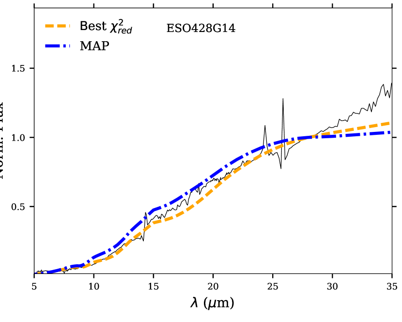
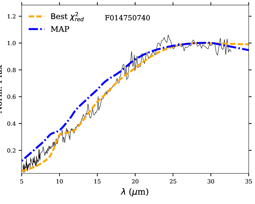
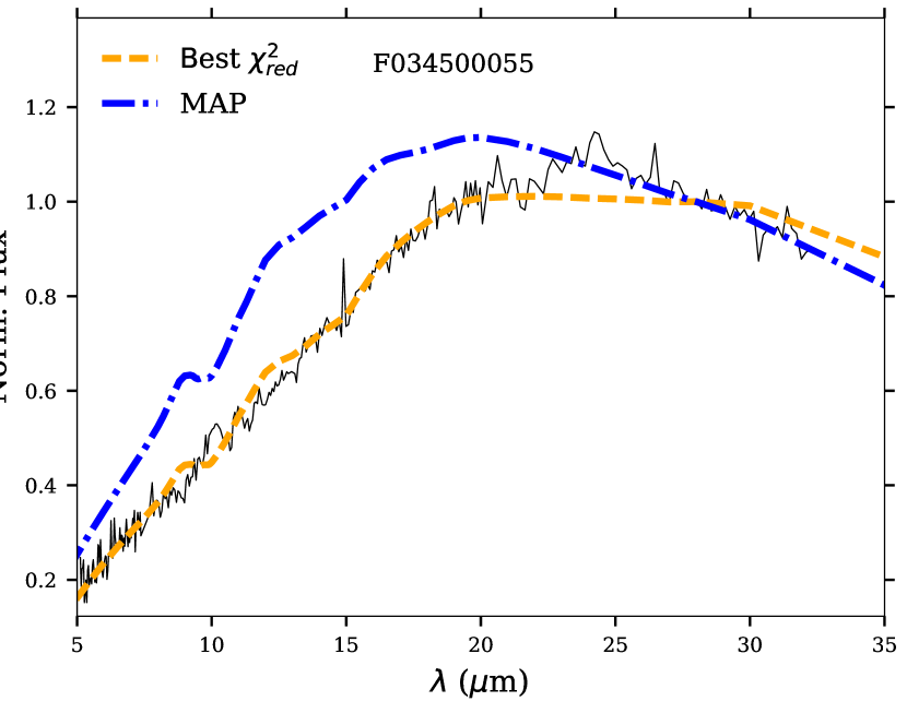
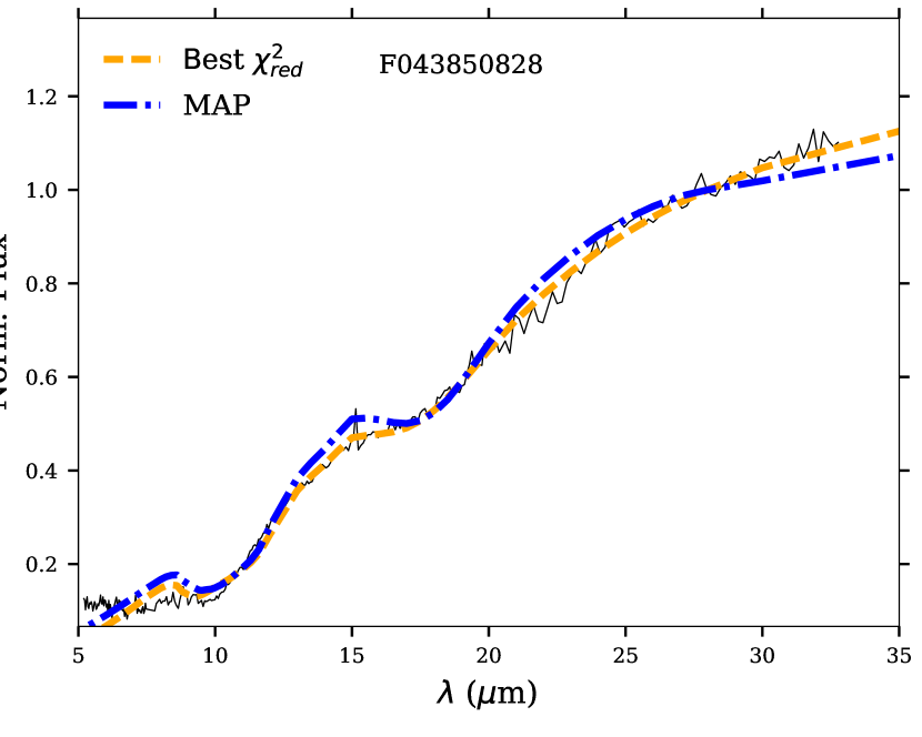
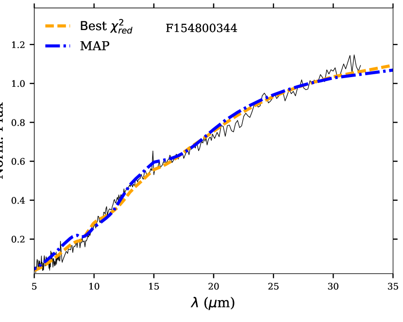
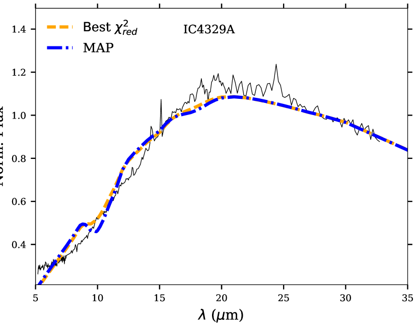
Figure C1: Individual fitting results. We present the adjusts for the best fit using ${\chi_{red}}^{2}$ (yellow dashed line) and the MAP (blue dotted-dashed line) distribution from BayesCLUMPY. The observed spectra and the SED models are normalized at 28$\mu$m.

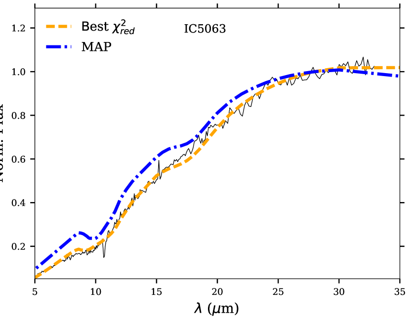
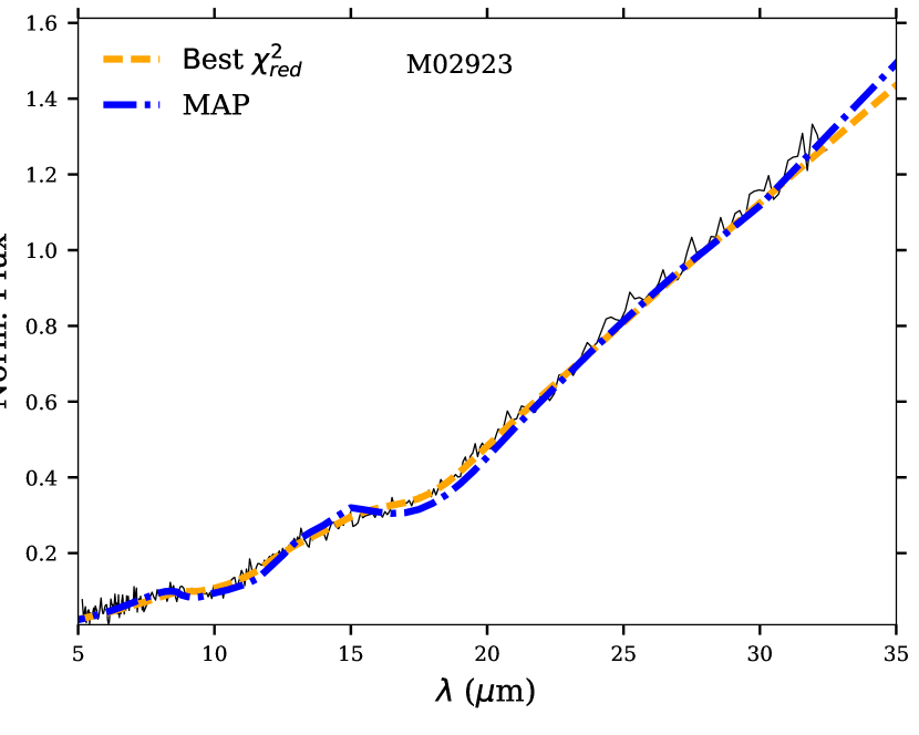
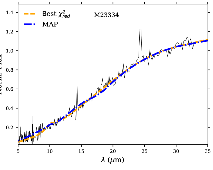
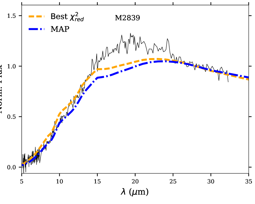
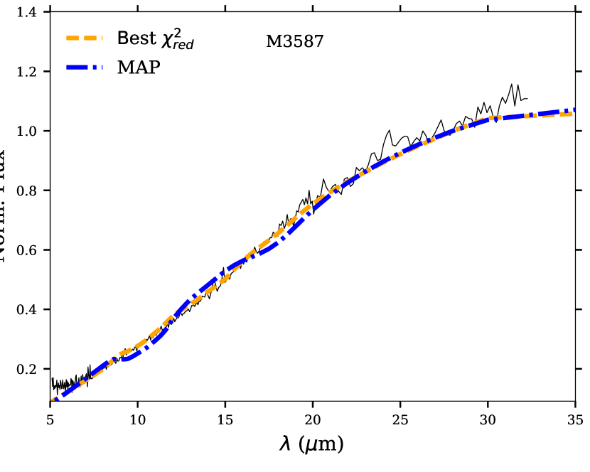
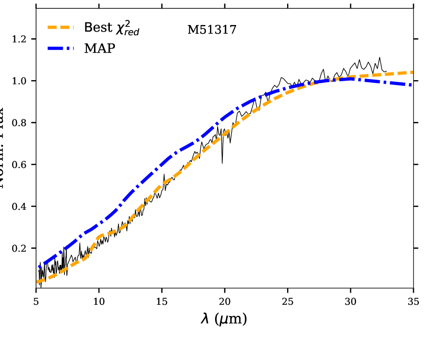
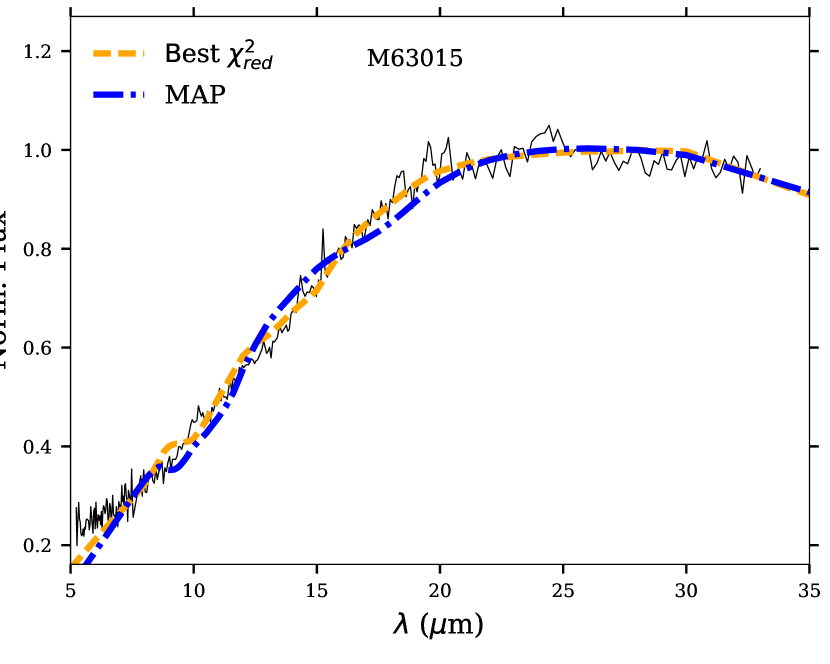
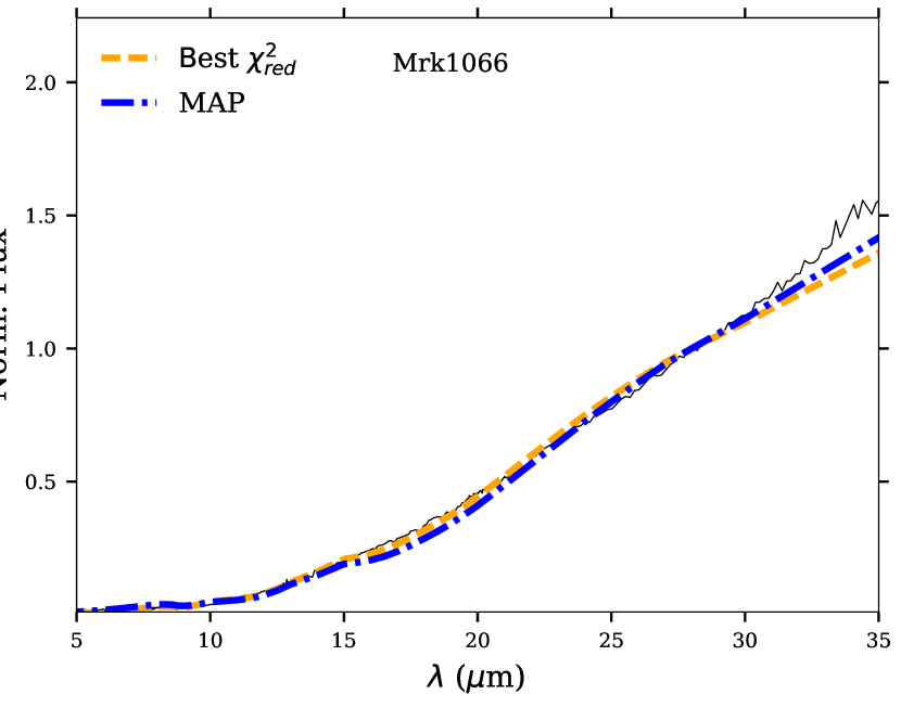
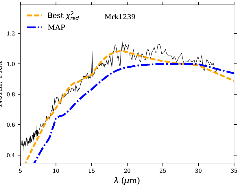
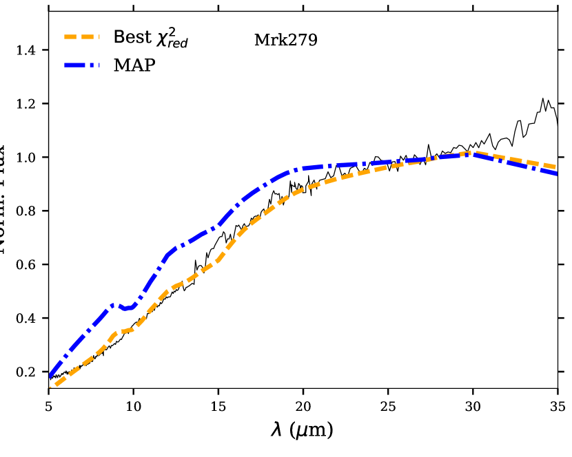
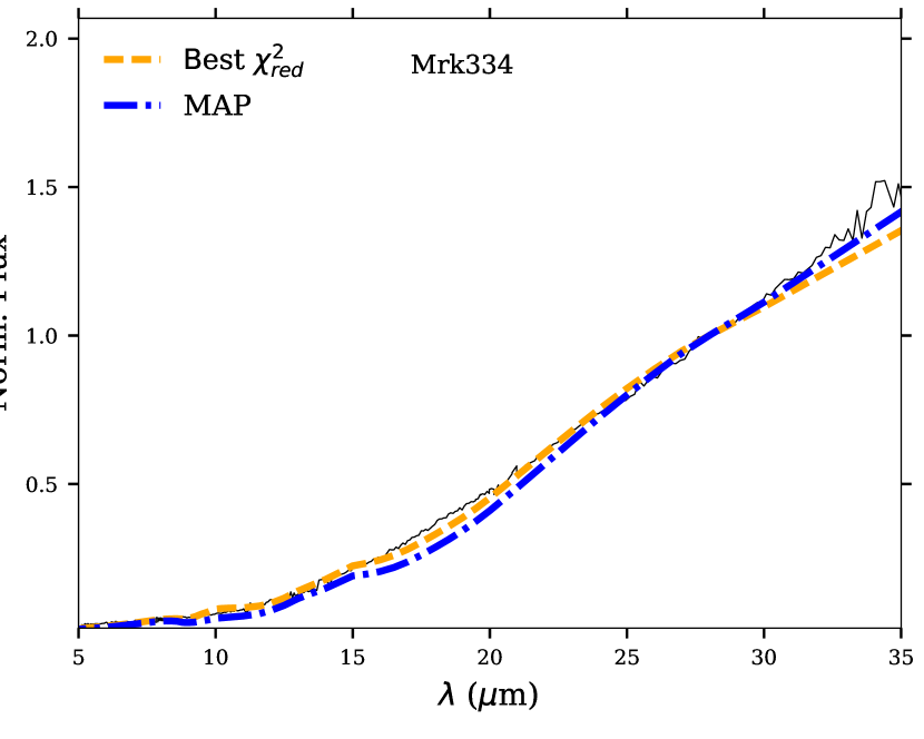
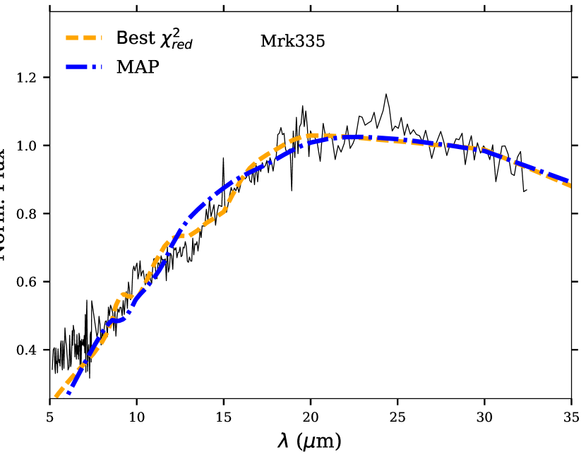
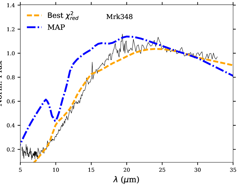
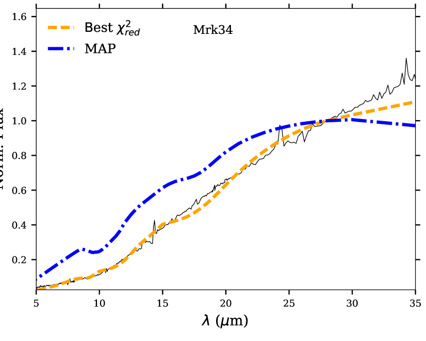
Figure C1: continued from previous page.

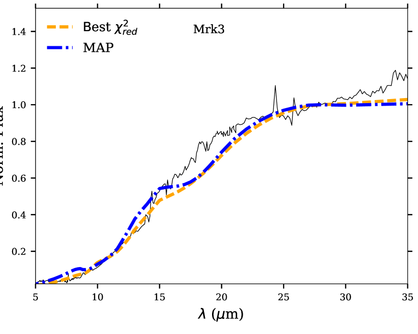
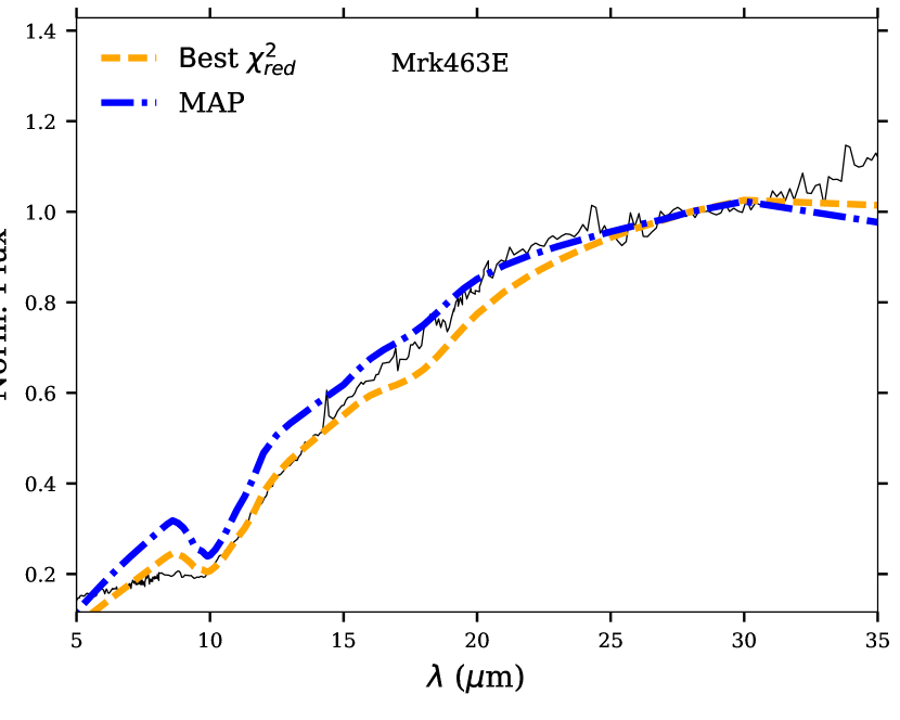
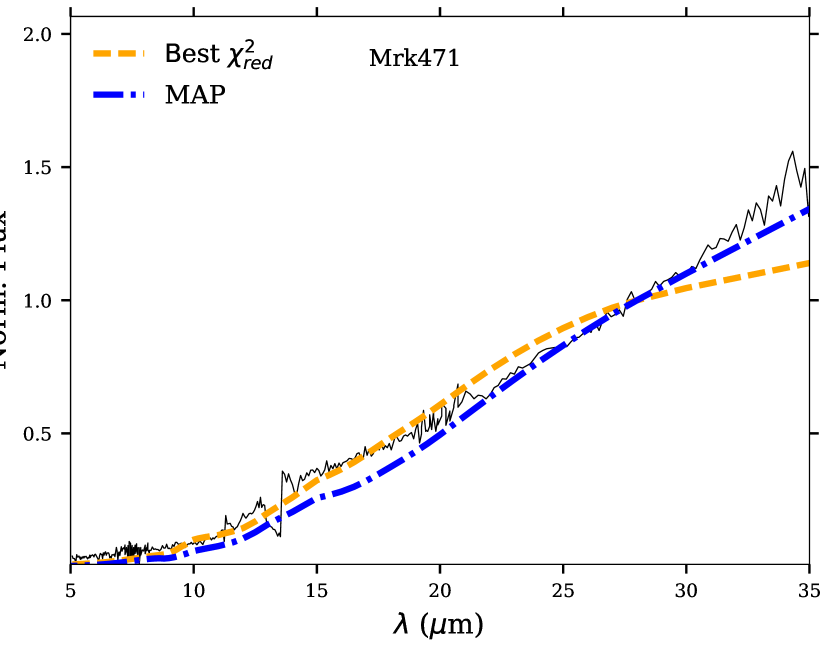
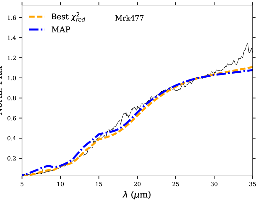
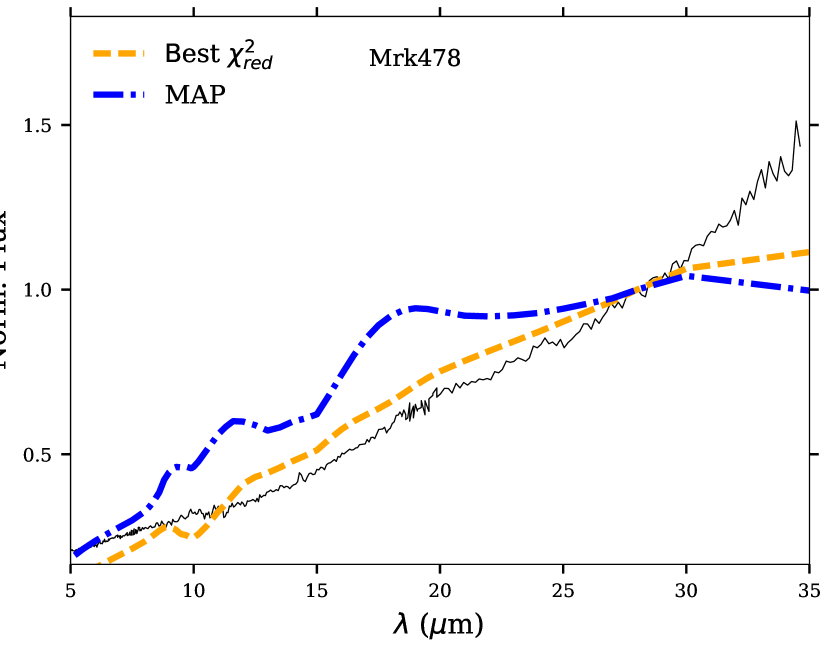
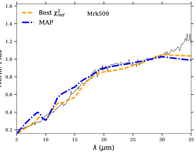
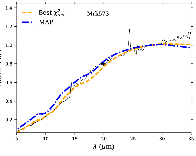
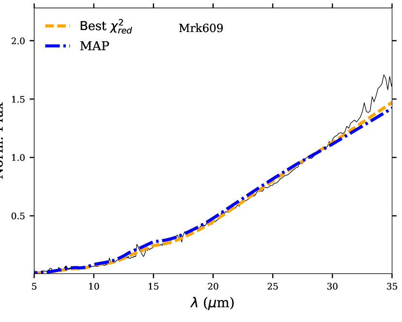
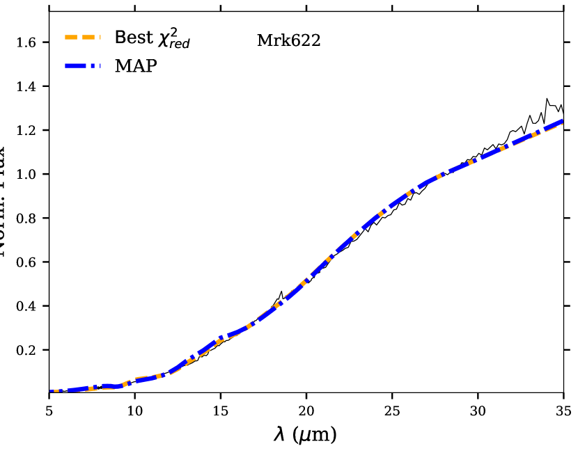
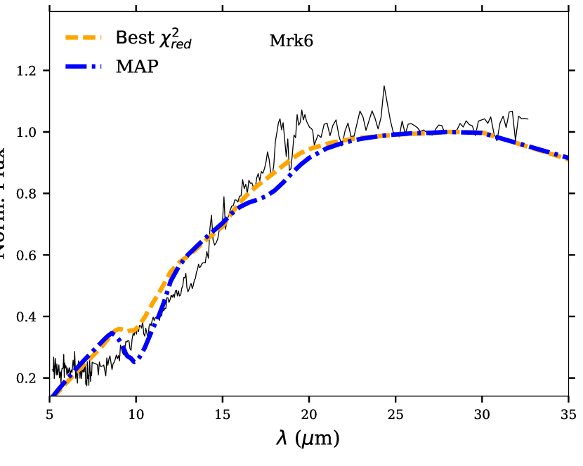
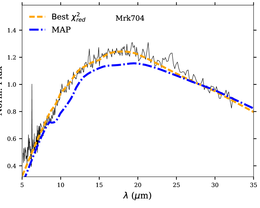
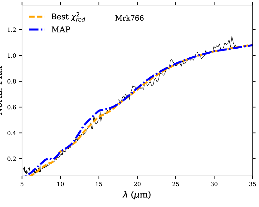
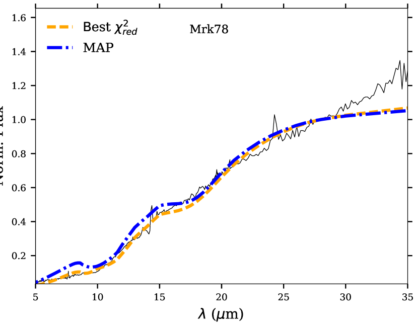
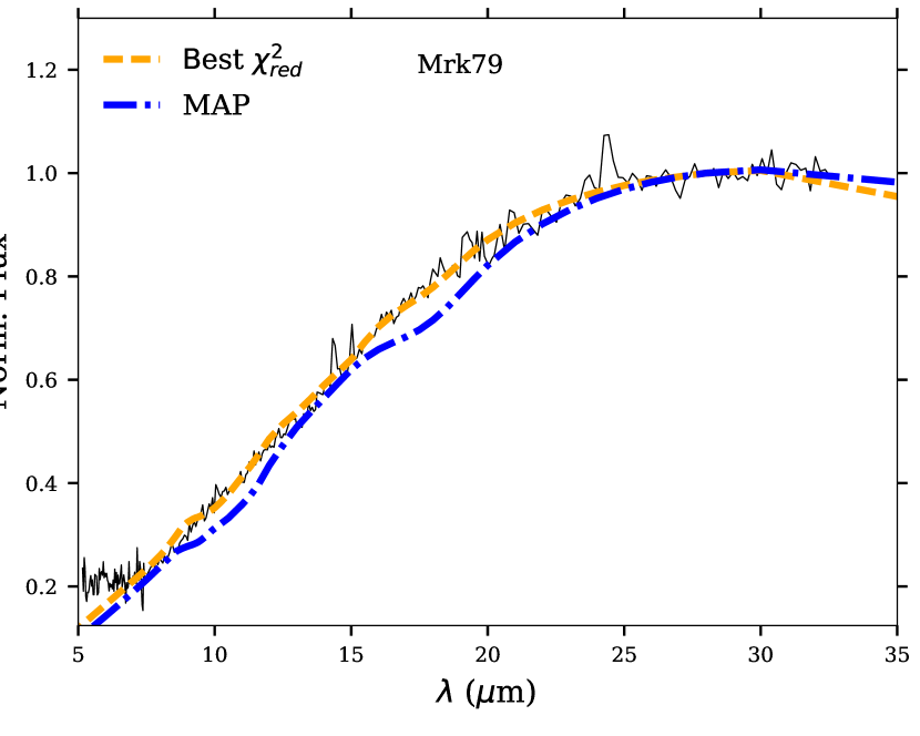
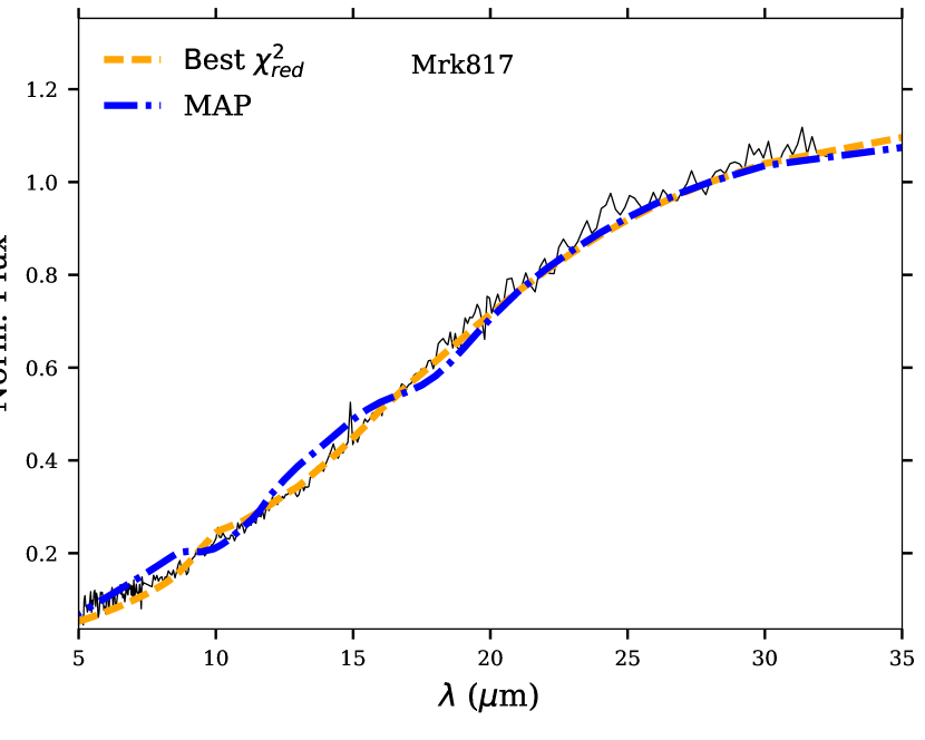
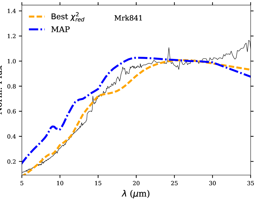
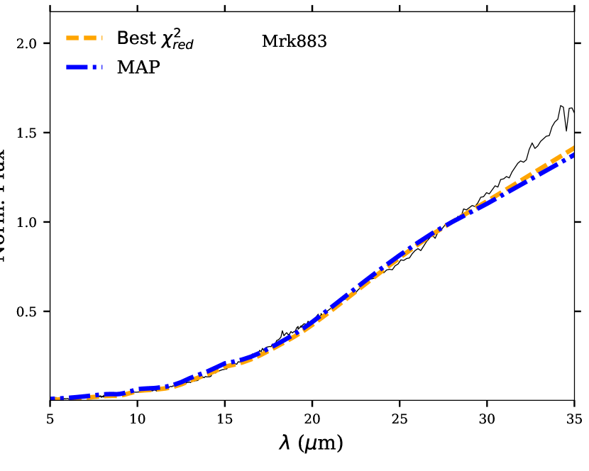
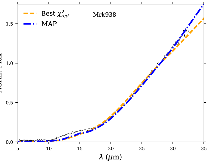
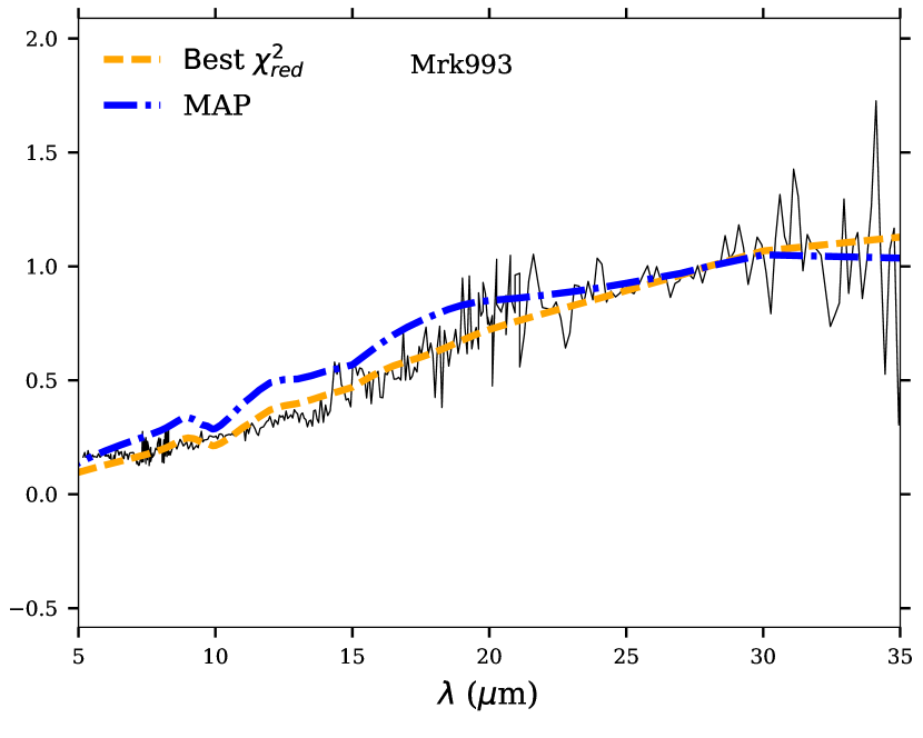
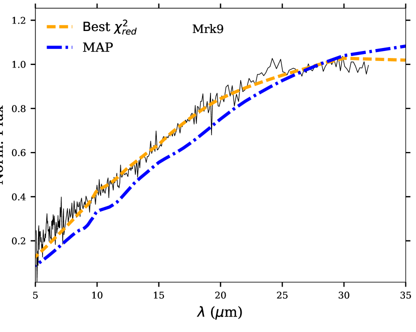
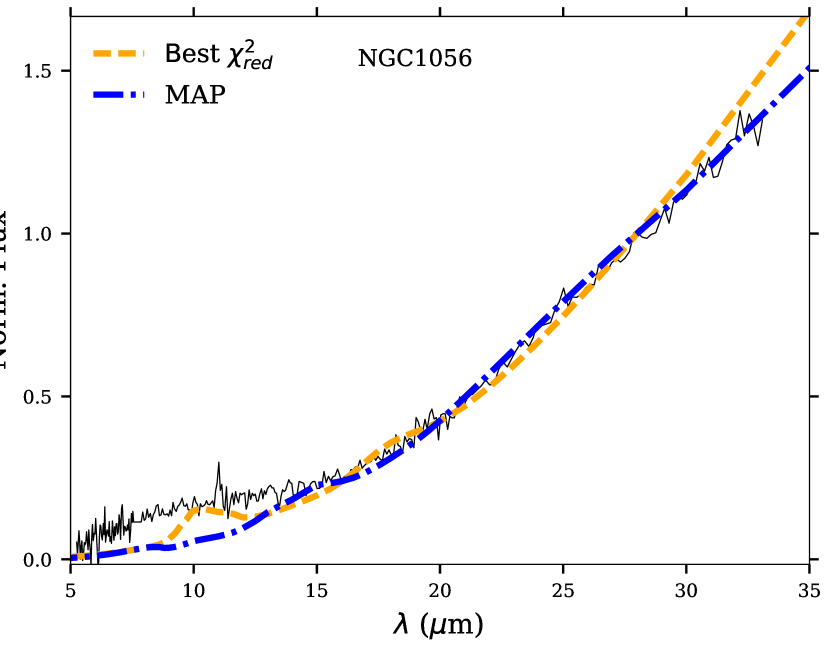
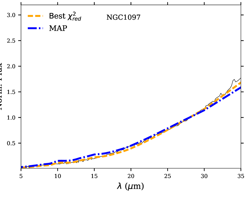
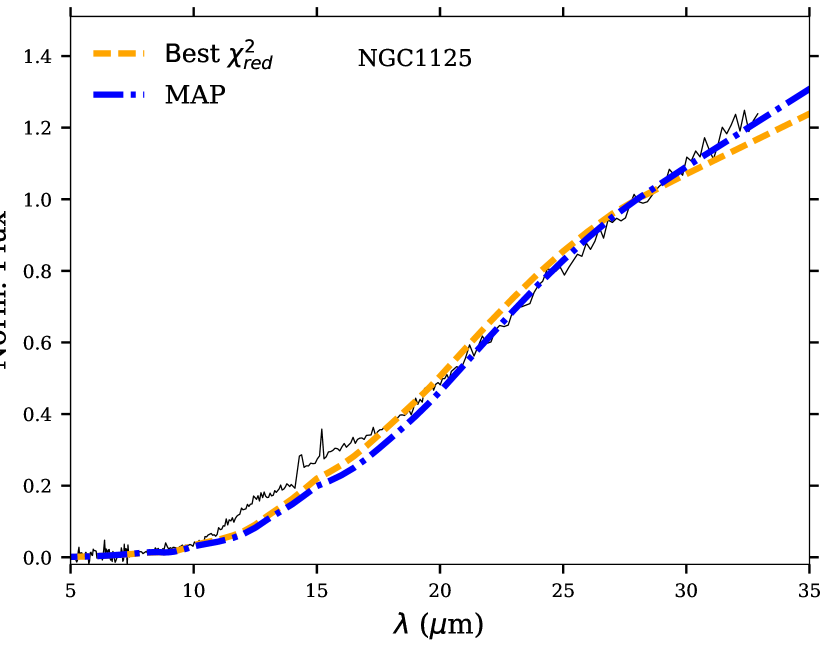
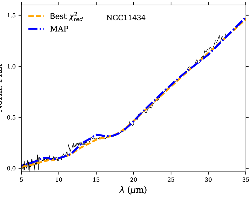
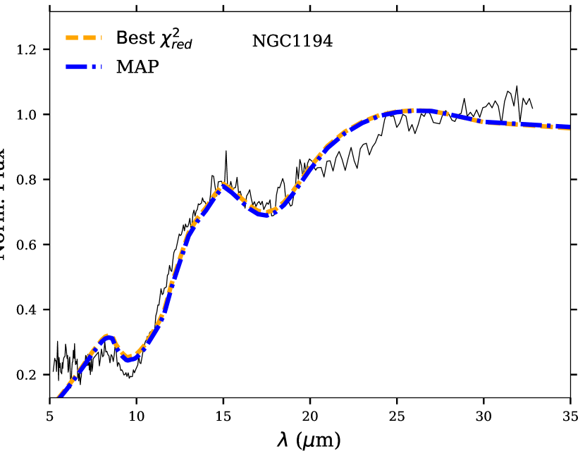
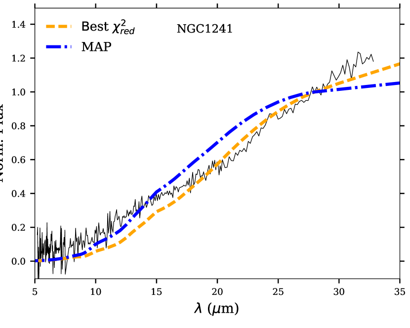
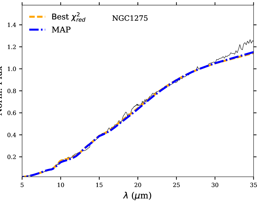
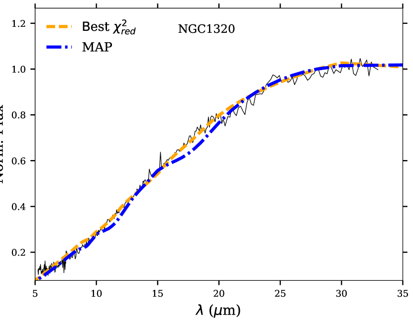
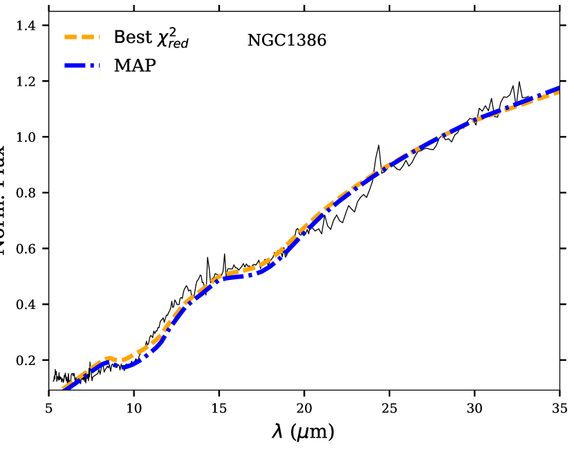
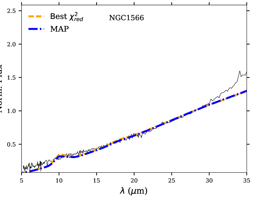
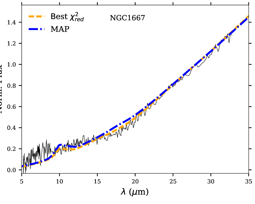
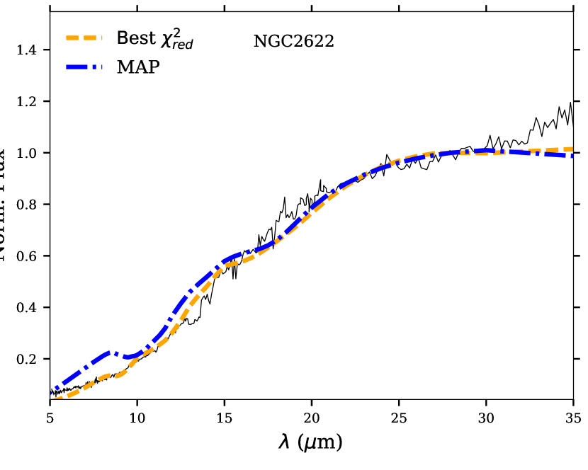
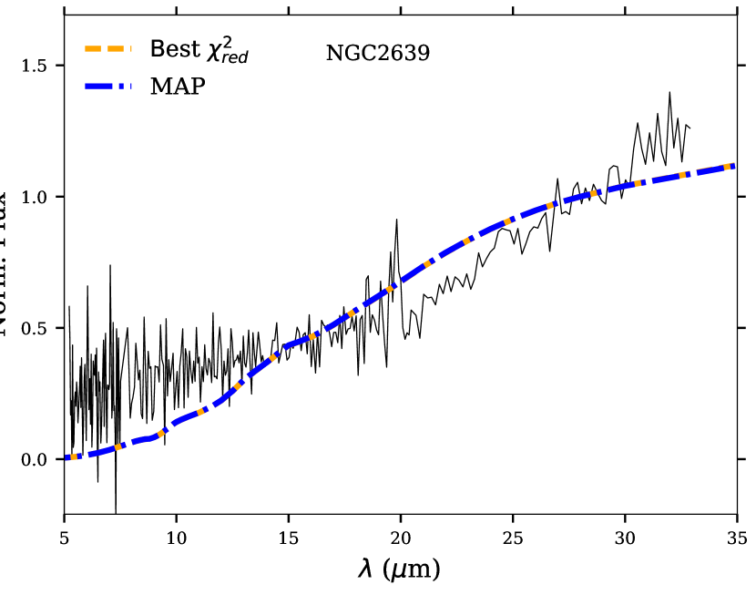
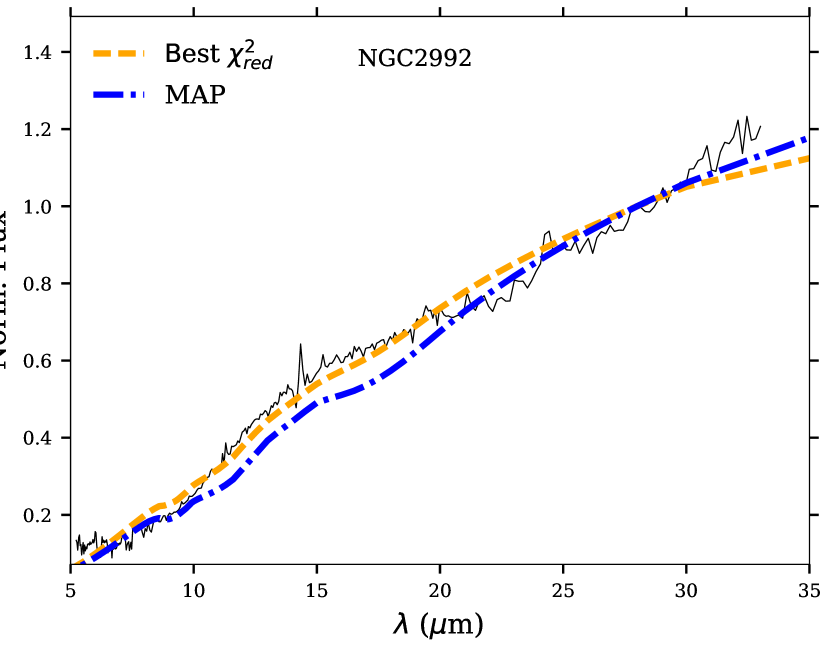
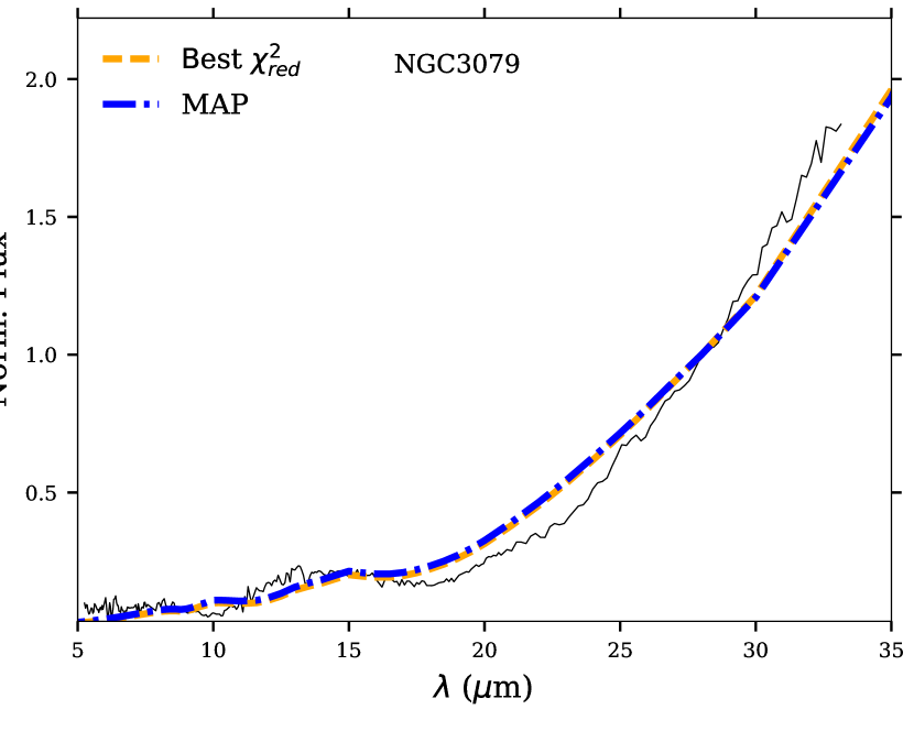
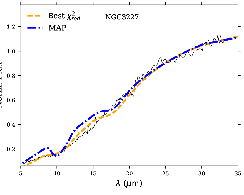
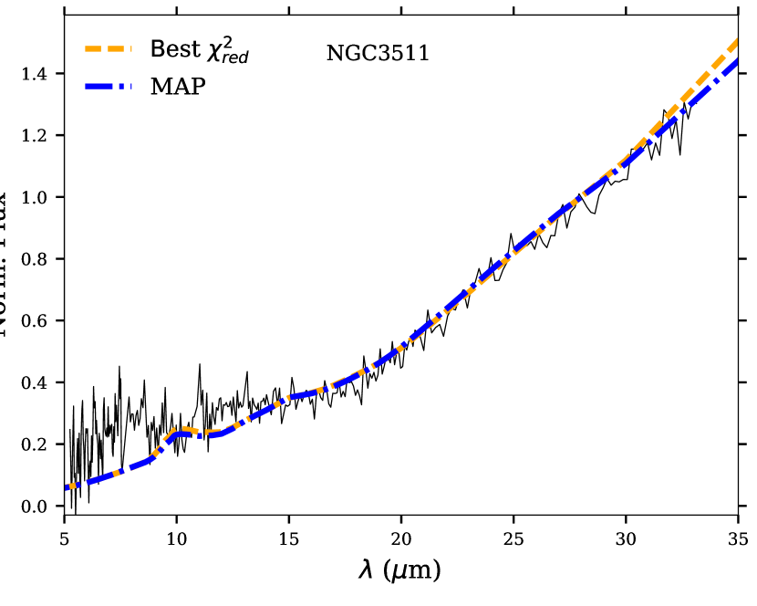
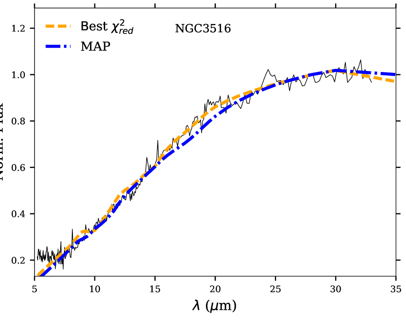
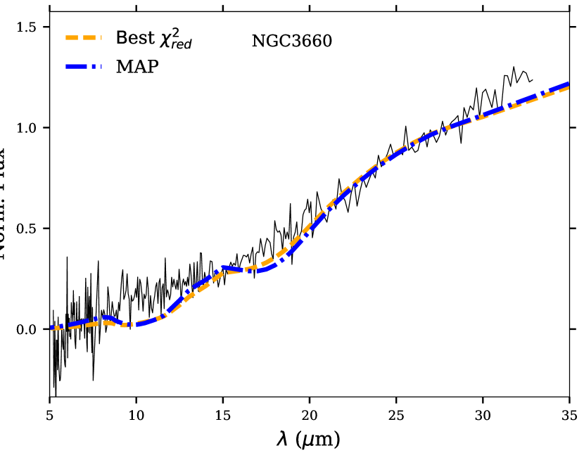
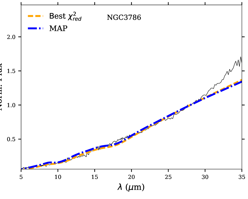
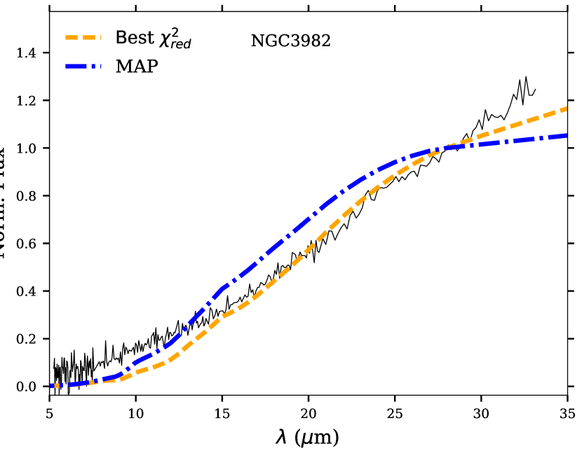
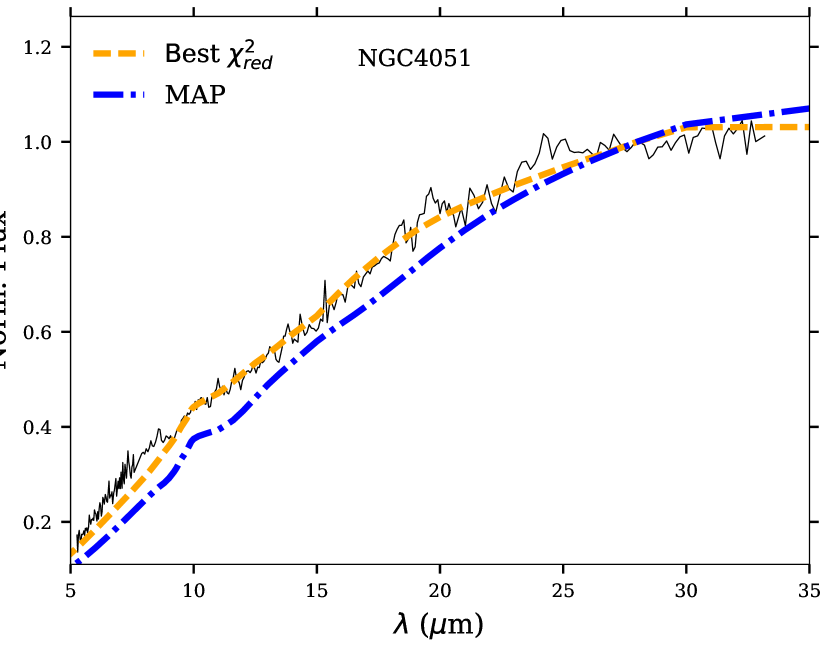
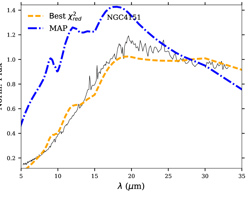
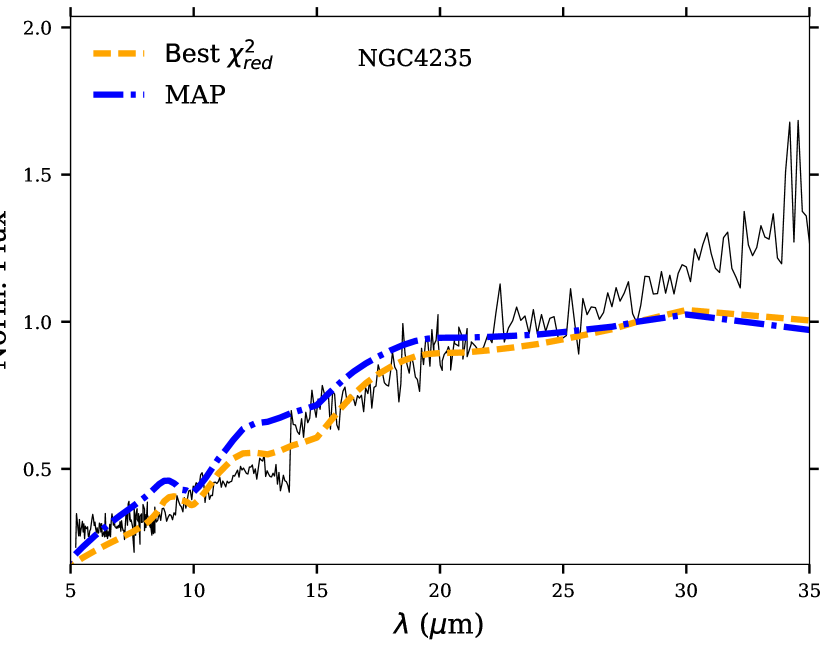
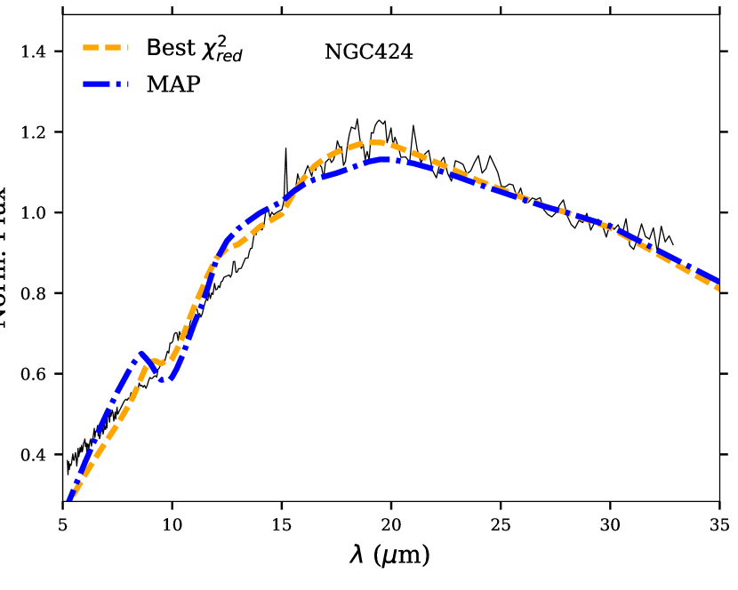
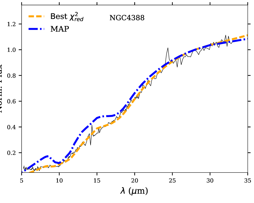
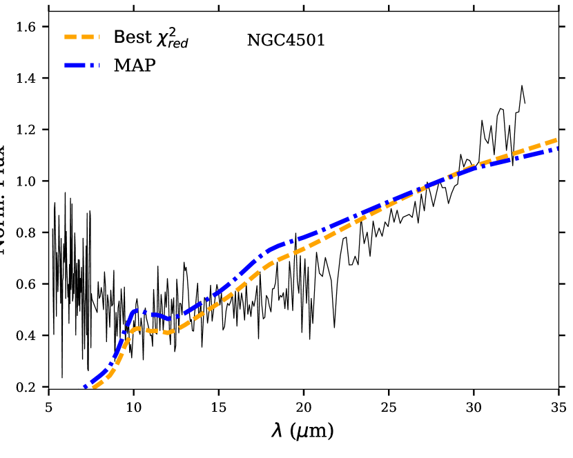
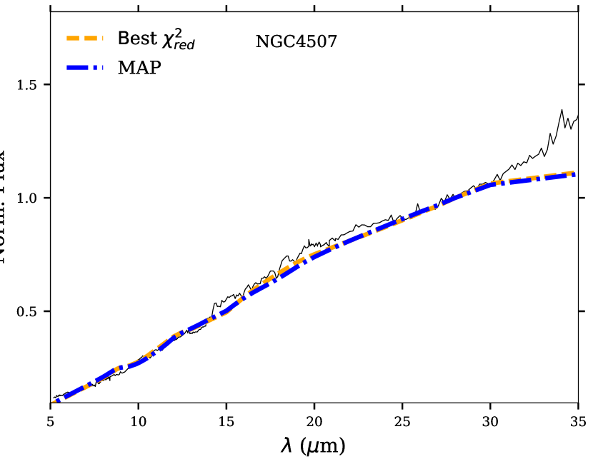
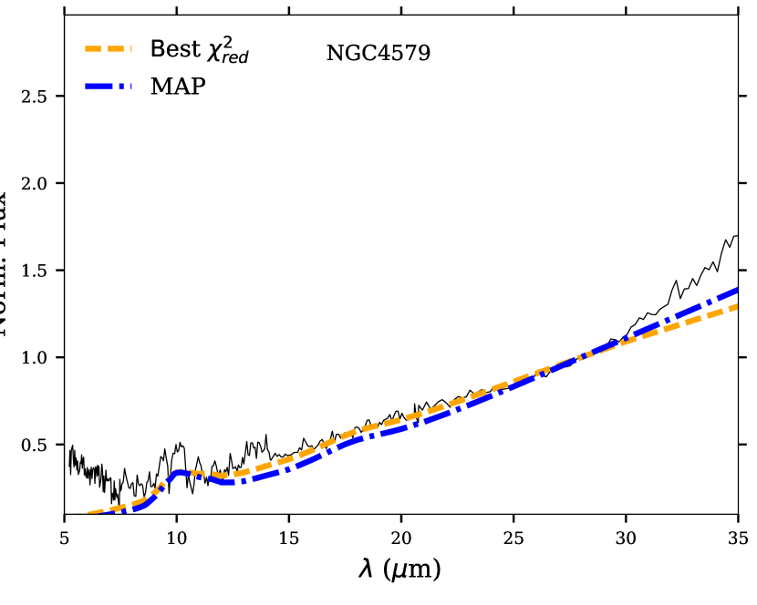
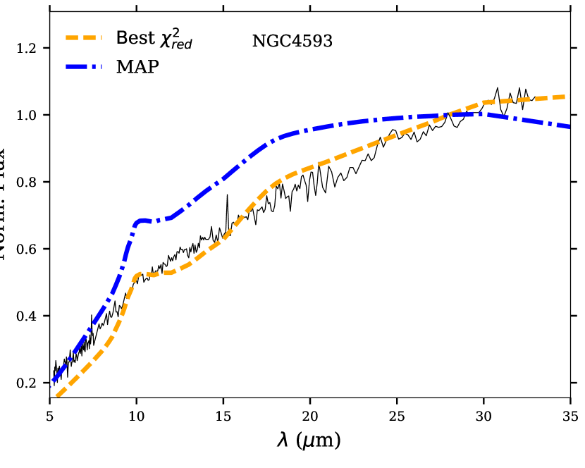
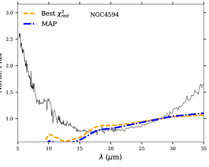
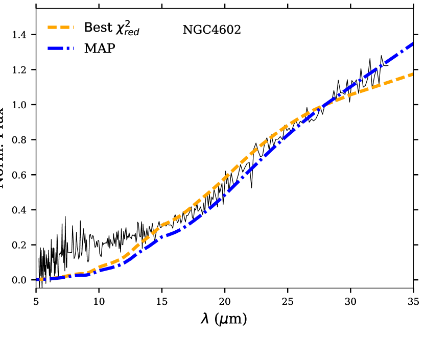
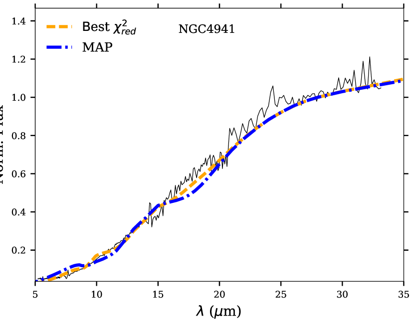
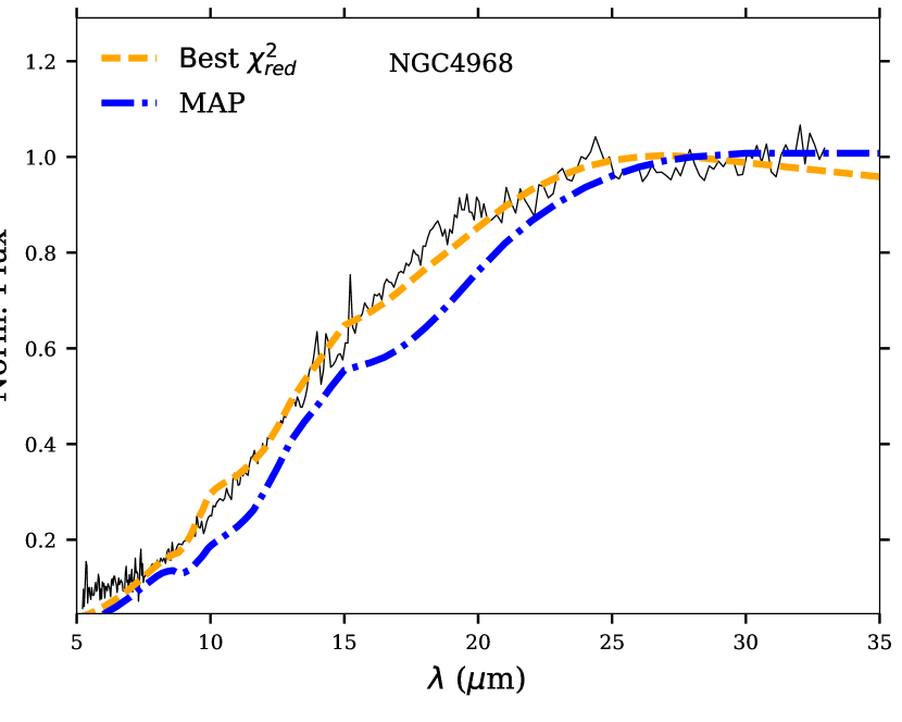
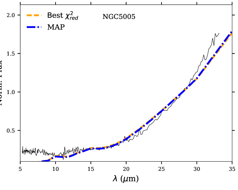
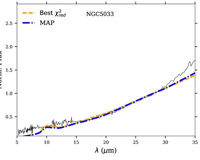
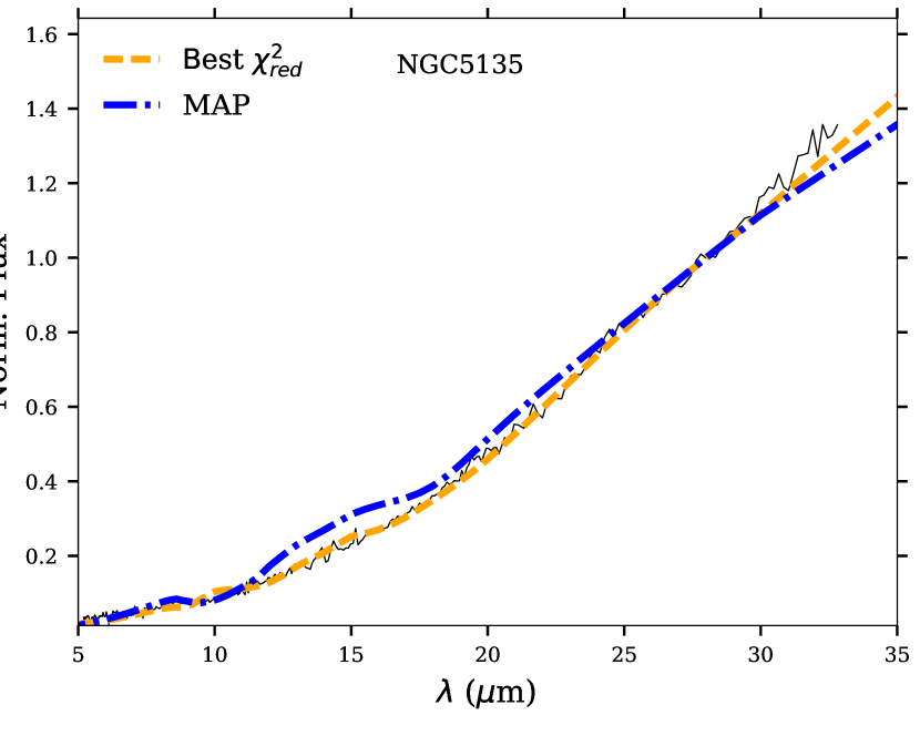
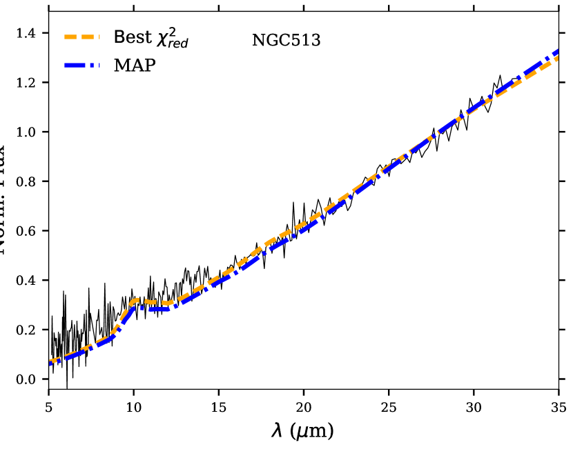
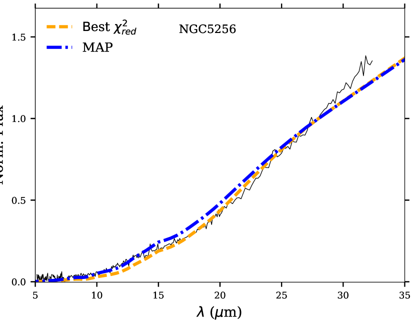
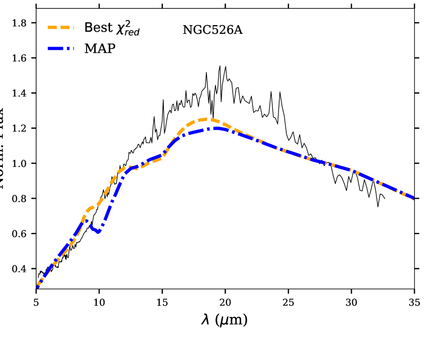
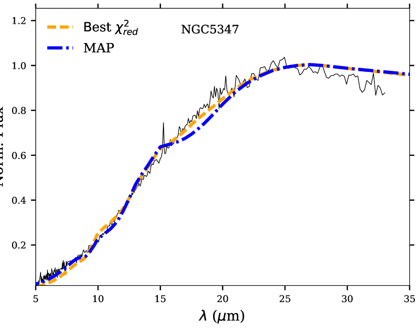
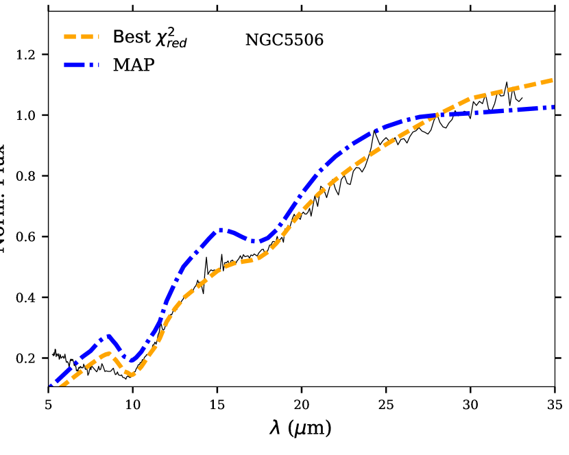
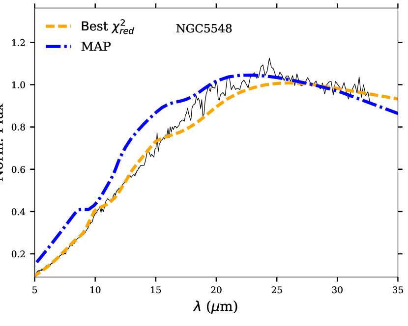
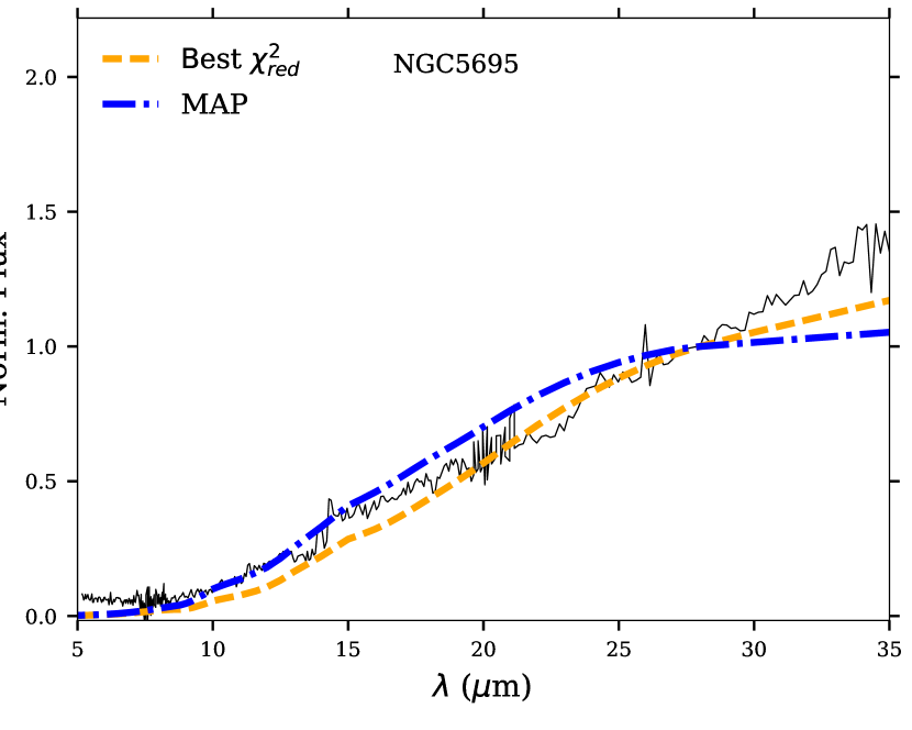
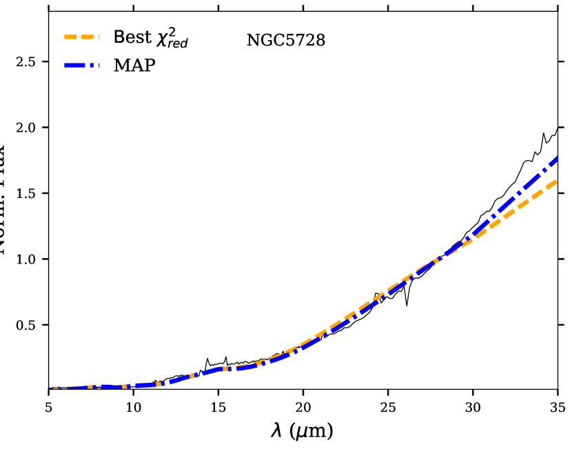
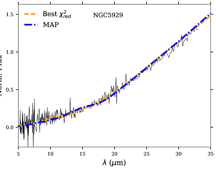
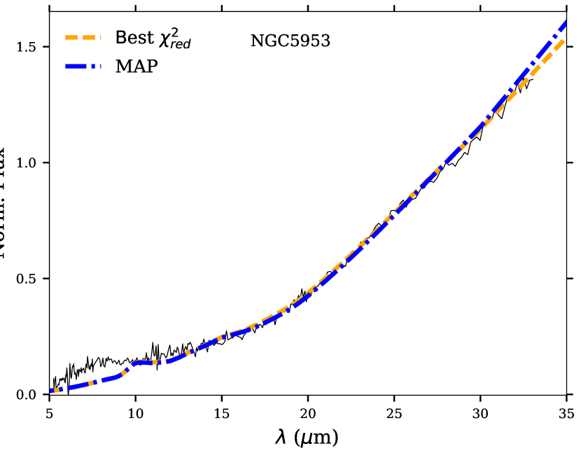
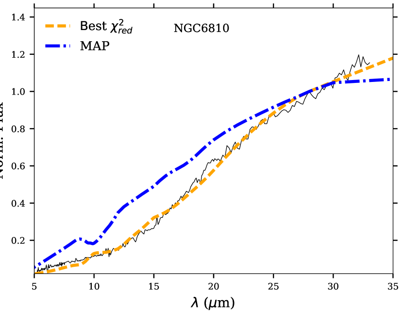
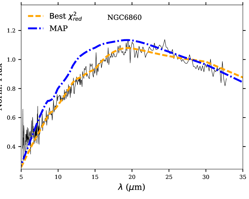
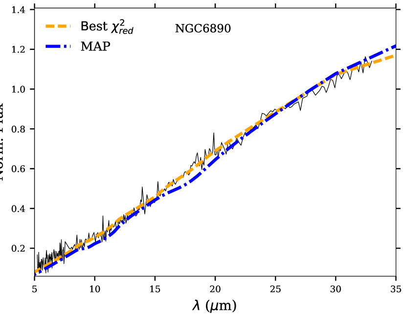
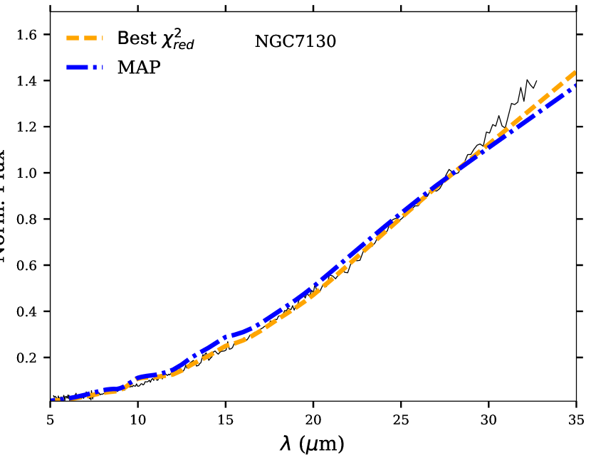
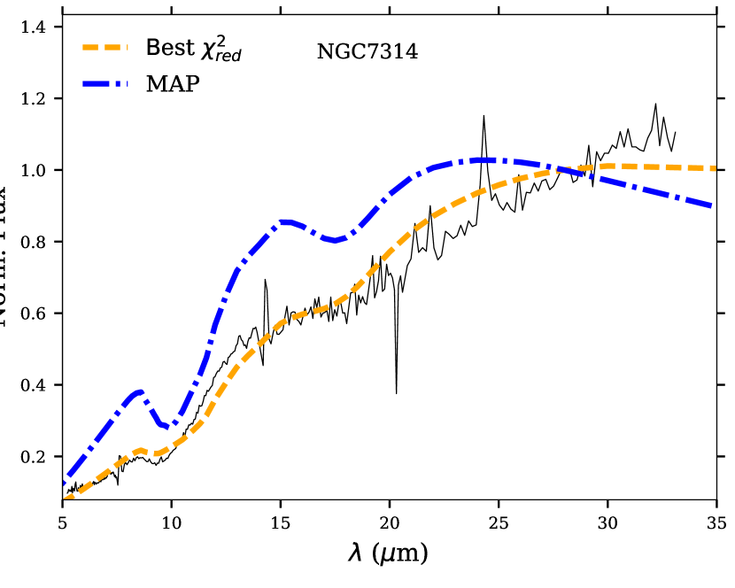
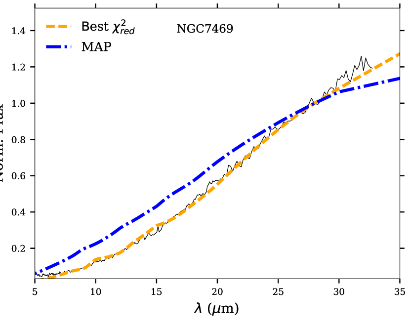
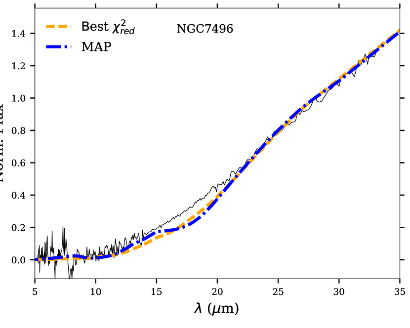
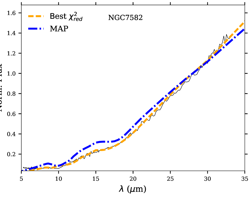
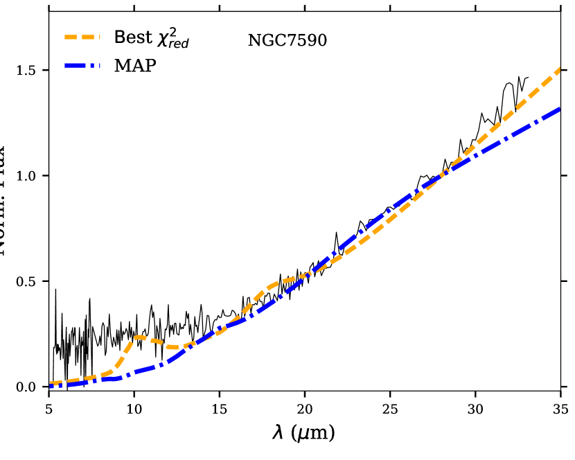
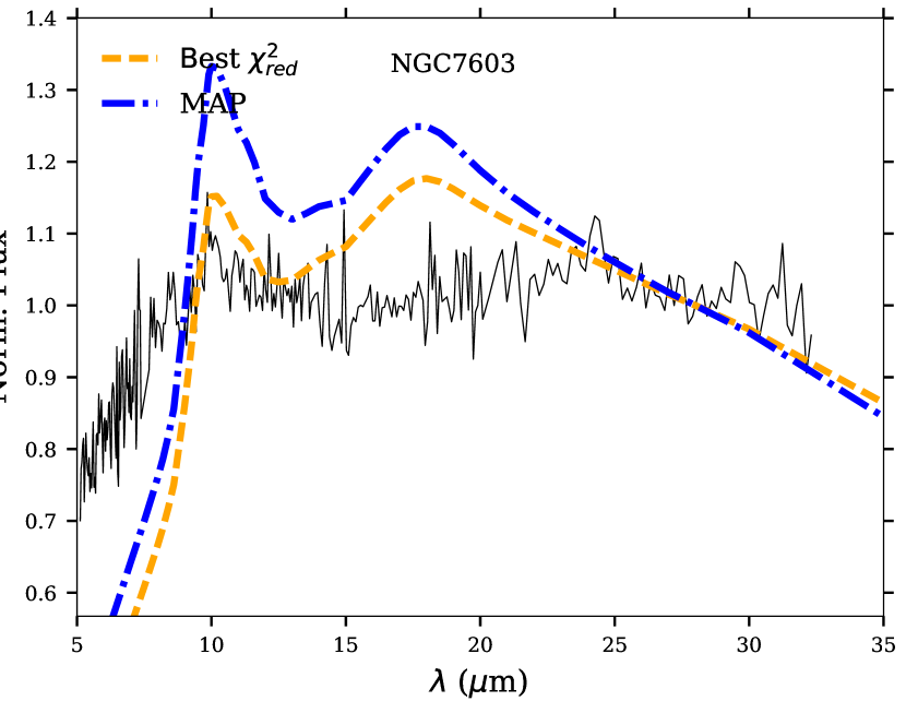
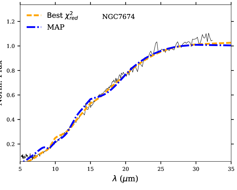
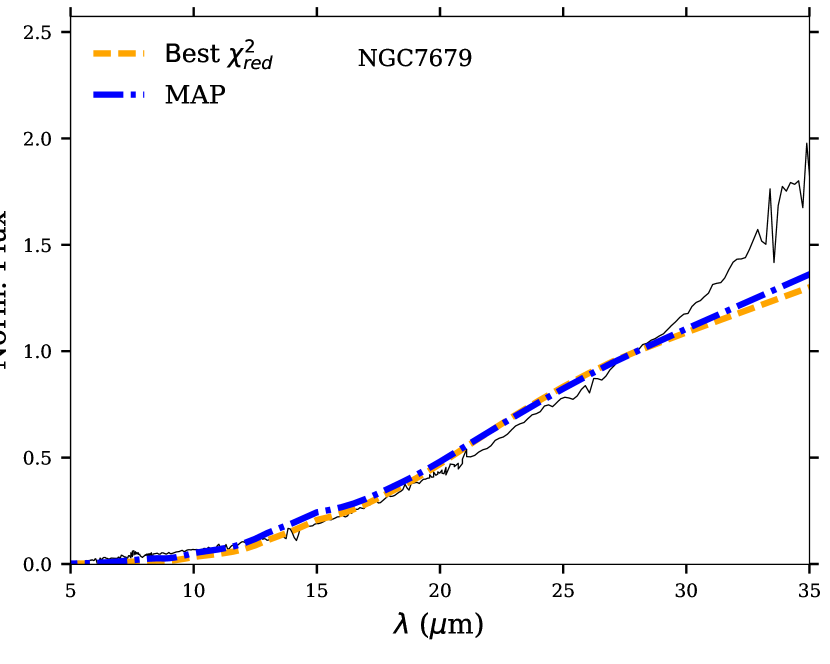
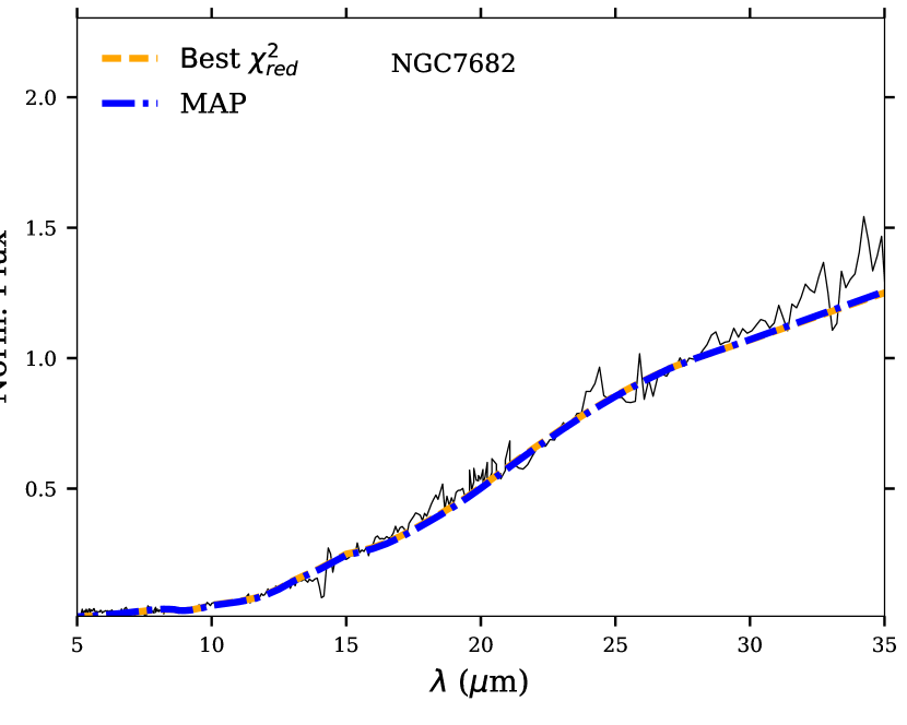
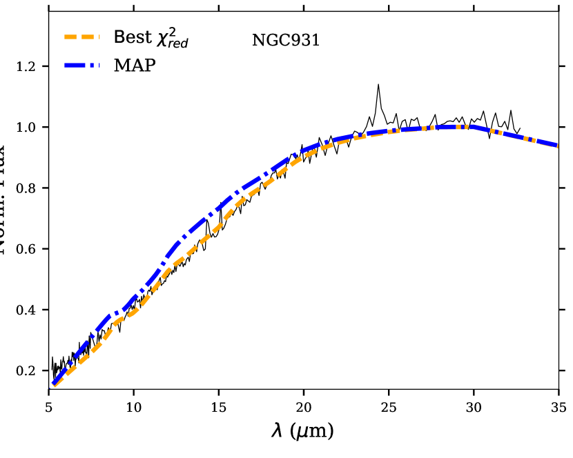
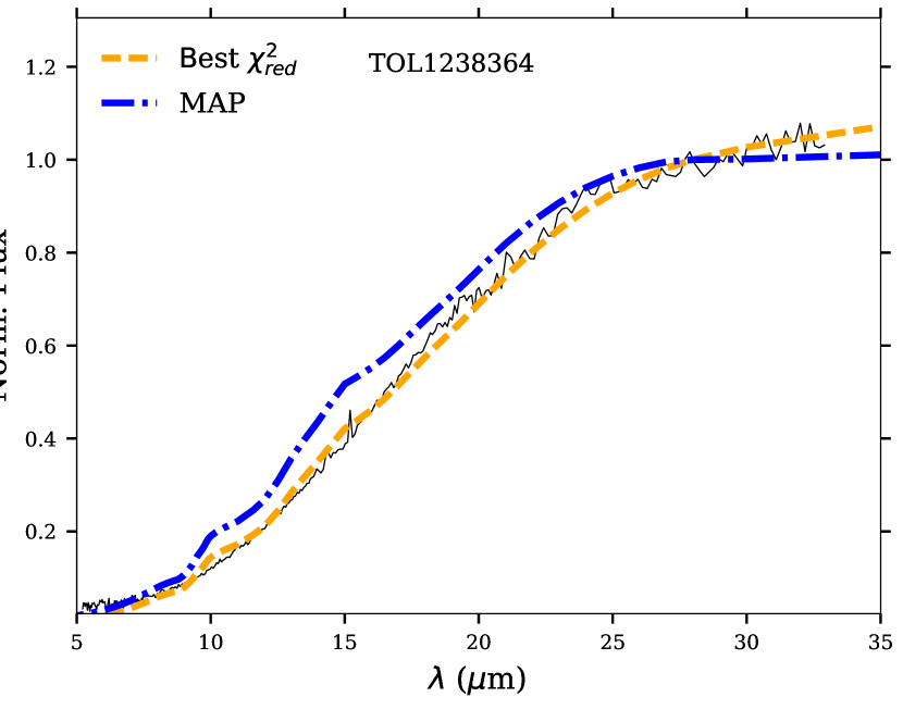
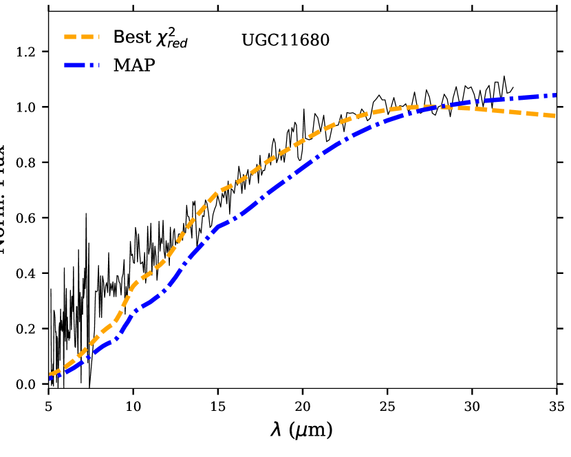
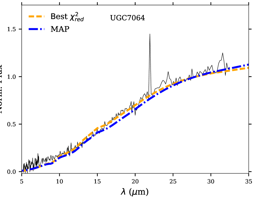
Figure C1: continued from previous page.

Figure C1: continued from previous page.

Figure C1: continued from previous page.

Figure C1: continued from previous page.

Figure C1: continued from previous page.

Figure C1: continued from previous page.

References

- Alonso-Herrero et al. (2011) Alonso-Herrero, A., Ramos Almeida, C., Mason, R., et al. 2011, ApJ, 736, 82
- Antonucci (1993) Antonucci, R. 1993, ARA&A, 31, 473
- Antonucci & Miller (1985) Antonucci, R. R. J., & Miller, J. S. 1985, ApJ, 297, 621
- Asensio Ramos & Ramos Almeida (2009) Asensio Ramos, A., & Ramos Almeida, C. 2009, ApJ, 696, 2075
- Asmus et al. (2011) Asmus D., Gandhi P., Smette A., Hönig S. F., Duschl W. J. 2011, A&A, 536, A36
- Barvainis (1987) Barvainis, R. 1987, ApJ, 320, 537
- Begelman et al. (1984) Begelman M. C., Blandford R. D., Rees M. J. 1984, Reviews of Modern Physics, 56, 255
- Bohlin, Savage & Drake (1978) Bohlin, R. C., Savage, B. D., & Drake, J. F. 1978, ApJ, 224, 132
- Buchanan et al. (2006) Buchanan, C. L., Gallimore, J. F., O’Dea, C. P., Baum, S. A., Axon, D. J., Robinson, A., Elitzur, M., & Elvis, M. 2006, AJ, 132, 401
- Burtscher et al. (2009) Burtscher, L., Jaffe, W., Raban, D., et al. 2009, ApJ, 705, L53
- Cid Fernandes et al. (2013) Cid Fernandes, R., et al., 2013, A&A, 557, A86
- Dadina (2007) Dadina M. 2007, A&A, 461, 1209
- Davies et al. (2012) Davies R., Burtscher L., Dodds-Eden K., Orban de Xivry G. 2012, JPhCS, 372, 2046
- Draine & Li (2001) Draine, B. T., & Li, A. 2001, ApJ, 551, 807
- Dullemond & van Bemmel (2005) Dullemond, C. P., & van Bemmel, I. M. 2005, A&A, 436, 47
- Efstathiou & Rowan-Robinson (1995) Efstathiou, A., & Rowan-Robinson, M. 1995, MNRAS, 273, 649
- Elitzur (2012) Elitzur, M. 2012, ApJ, 747, L33
- Elvis et al. (1994) Elvis, M., et al. 1994, ApJS, 95, 1
- Esquej et al. (2014) Esquej P. et al. 2014, ApJ, 780, 86
- Fritz et al. (2006) Fritz, J., Franceschini, A., & Hatziminaoglou, E. 2006, MNRAS, 366, 767
- Fuller et al. (2016) Fuller, L., Lopez-Rodriguez, E., Packham, et al. 2016, MNRAS, 462, 2618
- Gallimore et al. (2010) Gallimore, J. F., Yzaguirre, A., Jakoboski, J., et al. 2010, ApJS, 187, 172
- García-Burillo et al. (2014) García-Burillo S. et al. 2014, A&A, 567, A125
- García-Burillo et al. (2016) García-Burillo, S., Combes, F., Ramos Almeida, C., et al. 2016, ApJ, 823, 12
- Genzel & Cesarsky (2000) Genzel, R., & Cesarsky, C. J. 2000, ARA&A, 38, 761
- Gonzáles Delgado, Heckman & Leitherer (2001) González Delgado R. M., Heckman T. & Leitherer C. 2001, ApJ, 546, 845
- Granato & Danese (1994) Granato, G. L., & Danese, L. 1994, MNRAS, 268, 235
- Gratadour et al. (2015) Gratadour, D., Rouan, D., Grosset, L., Boccaletti, A. & Clénet, Y. 2015, A&A, 581, L8
- Hao et al. (2007) Hao, L., Weedman, D. W., Spoon, H. W. W., et al. 2007, ApJ, 655, L77
- Hernán-Caballero et al. (2015) Hernán-Caballero, A., et al. 2015, ApJ, 803, 109
- Ho (2009) Ho L. C., 2009, ApJ, 699, 626
- Hönig et al. (2006) Hönig, S. F., Beckert, T., Ohnaka, K., & Weigelt, G. 2006, A&A, 452, 459
- Houck et al. (2004) Houck J. R. et al., 2004, ApJS, 154, 18
- Ichikawa et al. (2015) Ichikawa, K., Packham, C., et al. 2015, ApJ, 803, 57
- Imanishi et al. (2016) Imanishi, M., Nakanishi, K. & Izumi, T. 2016 ApJ, 822, L10
- Ivezic et al. (1999) Ivezic, Z., Nenkova, M., & Elitzur, M. 1999, arXiv:astro-ph/9910475
- Jaffe et al. (2004) Jaffe W. et al. 2004, Nature, 429, 47
- Kennicutt et al. (2003) Kennicutt R. C. et al. 2003, PASP, 115, 928
- Krolik & Begelman (1988) Krolik, J. H., & Begelman, M. C. 1988, ApJ, 329, 702
- Lebouteiller et al. (2011) Lebouteiller, V., Barry, D. J., Spoon, H. W. W., Bernard-Salas, J., Sloan, G. C., Houck, J. R., Weedman, D. W. 2011, ApJS, 196, 8
- Lira et al. (2013) Lira, P., Videla, L., Wu, Y., Alonso-Herrero, A., Alexander, D., Ward, M. 2013, ApJ, 764, 59
- López-Gonzaga et al. (2014) López-Gonzaga, N., Jaffe, W., Burtscher, L., Tristram, K. R. W., & Meisenheimer, K. 2014, A&A, 565, A71
- Lutz et al. (2004) Lutz, D., Maiolino, R., Spoon, H. W. W., & Moorwood, A. F. M. 2004, A&A, 418, 465
- Lynden-Bell (1969) Lynden-Bell D. 1969, Nature, 223, 690
- Maiolino et al. (2007) Maiolino, R., Shemmer, O., Imanishi, M., Netzer, H., Oliva, E., Lutz, D. & Sturm, E. 2007, A&A, 468, 979
- Marinucci et al. (2012) Marinucci, A., Bianchi, S., Nicastro, F., Matt, G. & Goulding, A. D. 2012, ApJ, 748, 130
- Mason et al. (2009) Mason, R. E., Levenson, N. A., Shi, Y., Packham, C., Gorjian, V., Cleary, K., Rhee, J., Werner, M. 2009, ApJ, 693, 136
- Mason et al. (2015) Mason, R. E., Rodríguez-Ardila, A., Martins, L., Riffel, R., González-Martín et al. 2015, ApJS, 217, 13
- Mathis, Rumpl & Nordsieck (1977) Mathis, J. S., Rumpl, W., & Nordsieck, K. H. 1977, ApJ, 217, 425
- Mises (1964) Mises, von R. 1964, Mathematical Theory of Probability and Statistics (New York: Academic Press)
- Mor, Netzer & Elitzur (2009) Mor R., Netzer H., Elitzur M. 2009, ApJ, 705, 298
- Nikutta et al. (2009) Nikutta R., Elitzur M., Lacy M. 2009, ApJ, 707, 1550
- Nenkova et al. (2002) Nenkova, M., Ivezić, Ž., & Elitzur, M. 2002, ApJ, 570, L9
- Nenkova et al. (2008a) Nenkova, M., Sirocky, M. M., Ivezić, Ž., & Elitzur, M. 2008, ApJ, 685, 147
- Nenkova et al. (2008b) Nenkova, M., Sirocky, M. M., Nikutta, R., Ivezić, Ž., & Elitzur, M. 2008, ApJ, 685, 160
- Netzer et al. (2007) Netzer, H., Lutz, D., Schweitzer, M., et al. 2007, ApJ, 666, 806
- Netzer et al. (2015) Netzer H., 2015, ARA&A, 53, 365
- Pérez García & Rodríguez Espinosa (2001) Pérez García A. M. & Rodríguez Espinosa J. M. 2001, ApJ, 557, 39
- Pier & Krolik (1992) Pier, E. A., & Krolik, J. H. 1992, ApJ, 401, 99
- Pogge (1988) Pogge, R. W. 1988, ApJ, 328, 519
- Raban et al. (2009) Raban, D., Jaffe, W., Röttgering, H., Meisenheimer, K., & Tristram, K. 2009, MNRAS, 394, 1325
- Ramos Almeida et al. (2009) Ramos Almeida C. et al. 2009, ApJ, 702, 1127
- Ramos Almeida et al. (2011) Ramos Almeida, C., Levenson, N. A., Alonso-Herrero, A., et al. 2011, ApJ, 731, 92
- Ramos Almeida et al. (2014) Ramos Almeida, C., Alonso-Herrero, A., Levenson, N., Asensio Ramos, A., et al. 2014, MNRAS, 439, 3847
- Riffel et al. (2006) Riffel R., Rodríguez-Ardila A. & Pastoriza, M. G., 2006, A&A, 457, 61
- Riffel et al. (2009) Riffel, R., Pastoriza, M. G., Rodríguez-Ardila, A., & Bonatto, C. 2009, MNRAS, 400, 273
- Rodríguez-Ardila & Viegas (2003) Rodríguez-Ardila A. & Viegas S. M. 2003, MNRAS, 340, L33
- Rodríguez-Ardila & Mazzaly (2006) Rodríguez-Ardila, A. & Mazzaly, Z., 2006, MNRAS, 367, L57
- Ruschel-Dutra et al. (2014) Ruschel-Dutra, D., Pastoriza, M., Riffel, R., Sales, D. A., & Winge, C. 2014, MNRAS, 108
- Sales et al. (2010) Sales, D. A., Pastoriza, M. G., & Riffel, R. 2010, ApJ, 725, 605
- Sales et al. (2013) Sales, D. A., Pastoriza, M. G., Riffel, R., & Winge, C. 2013, MNRAS, 429, 2634
- Sales et al. (2014) Sales D. A., Ruschel-Dutra D., Pastoriza M. G., Riffel R., Winge C. 2014, MNRAS, 441, 630
- Sanders et al. (2003) Sanders, D. B., Mazzarella, J. M., Kim, D.C., Surace, J. A., & Soifer, B. T. 2003, AJ, 126, 1607
- Schartmann et al. (2008) Schartmann, M., Meisenheimer, K., Camenzind, M., et al. 2008, A&A, 482, 67
- Siebenmorgen et al. (2004) Siebenmorgen, R., Krügel, E., Spoon, H. W. W. 2004, A&A, 414, 123
- Smith et al. (2007a) Smith, J. D. T., Armus, L., Dale, D. A., et al. 2007, PASP, 119, 1133
- Smith et al. (2007b) Smith, J. D. T., Draine, B. T., Dale, D. A., et al. 2007, ApJ, 656, 770
- Stalevski et al. (2012) Stalevski, M., Fritz, J., Baes, M., Nakos, T., & Popović, L. Č. 2012, MNRAS, 420, 2756
- Storchi-Bergmann & Bonatto (1991) Storchi-Bergmann, T., & Bonatto, C. J. 1991, MNRAS, 250, 138
- Storchi-Bergmann et al. (1992) Storchi-Bergmann, T., Wilson, A. S., & Baldwin, J. A. 1992, ApJ, 396, 45
- Sturm et al. (2006) Sturm, E., Hasinger, G., Lehmann, I., Mainieri, V., Genzel, R., Lehnert, M. D., Lutz, D., & Tacconi, L. J. 2006, ApJ, 642, 81
- Tran et al. (1992) Tran, H. D., Miller, J. S., & Kay, L. E. 1992, ApJ, 397, 452
- Tran (1995) Tran, H. D. 1995, ApJ, 440, 565
- Tristram et al. (2007) Tristram, K. R. W., Meisenheimer, K., Jaffe, W., et al. 2007, A&A, 474, 837
- Tristram et al. (2009) Tristram, K. R. W., et al., 2009, A&A, 502, 67
- Tristram et al. (2014) Tristram, K. R. W., Burtscher, L., Jaffe, W., Meisenheimer, K., Hönig, S. F., Kishimoto, M., Schartmann, M., & Weigelt, G. 2014, A&A, 563, A82
- Urry & Padovani (1995) Urry, C. M., & Padovani, P. 1995, PASP, 107, 803
- Vasudevan et al. (2010) Vasudevan, R. V., Fabian, A. C., Gandhi, P., Winter, L. M. & Mushotzky, R. F. 2010, MNRAS, 402, 1081
- Whittle (1992) Whittle, M. 1992, ApJS, 79, 49
- Wu et al. (2009) Wu, Y., Charmandaris, V., Huang, J., Spinoglio, L., & Tommasin, S. 2009, ApJ, 701, 658