A Nondeterministic Model for Abstract Geometrical Computation

Abstract

A signal machine is an abstract geometrical model for compu- tation, proposed as an extension to the one-dimensional cellular automata, in which discrete time and space of cellular automata is replaced with continuous time and space in signal machine. A signal machine is defined as a set of meta-signals and a set of rules. A signal machine starts from an initial configuration which is a set of moving signals. Signals are moving in space freely until a collision. Rules of signal machine specify what happens after a collision, or in other words, specify out-coming signals for each set of colliding signals. Originally signal machine is defined by its rule as a deterministic machine. In this paper, we introduce the concept of non-deterministic signal machine, which may contain more than one defined rule for each set of colliding signals. We show that for a specific class of nondeterministic signal machines, called $k$-restricted nondeterministic signal machine, there is a deterministic signal machine computing the same result as the nondeterministic one, on any given initial configuration. $k$-restricted nondeterministic signal machine is a nondeterministic signal machine which accepts an input iff produces a special accepting signal, which have at most two nondeterministic rule for each collision, and at most $k$ collisions before any acceptance.

1 Introduction

Consider some colored particles moving on a line with constant speeds. Some particles may have zero speed and do not move. When two or more particles collide, particles are replaced with some new colored particles, according to predefined rules of the signal machine. Suppose that you are given some colored particles with their initial position on a line and collision rules, and you are asked to drawing the space-time diagram of the movement of these particles, until no more collision may happen. Signal machines are such dynamical systems, were signals are traces of particles in space-time diagram. The signal machine model is an Abstract Geometrical Computation (AGC) model dealing with Euclidean geometry which introduced in 2003 by Jerome-Durand Lose for the first time [5]. Signal machines are originally introduced as a continues extension of one-dimensional cellular automata in time and space [10]. Signals in a signal machine are moving independently, thus, signal machines are inherently parallel and they can viewed as a massively parallel computational model [3].

Signal machines are able to simulate any Turing-Computation and they are Turing-Universal [6]. With continuous time, they can be used to decide (in finite time) recursively enumerable problems using the black-hole principle [6, 7]. They are also capable of analog computation by using the continuity of space and time to simulate analog models such as BSS [8, 9]. To achieve massive parallelism, a fractal tree construction technique is provided on signal machine, and it is used to solve the satisfiability of quantified Boolean formula (Q-SAT) problem, the classic PSPACE-complete problem, in bounded space and time [4].

All studies on signal machines are on deterministic version of signal machines. However, on every computational model, studying the non-deterministic versions of computation and theirs computability power is an important concept. One important question which arises is that if nondeterminism brings more power to the considered computational model. To this end, the problem of comparing computational power of nondeterministic and deterministic signal machines is not investigated yet.

In this paper, first we define nondeterministic signal machine as a signal machine which may have more than one rule applicable for each collision from which one is nondeterministically selected to be applied. Then, we show that the nondeterminism does not improve computability power of signal machines, for a specific class of signal machines. For this purpose we use a constructive proof. In other words, we propose an algorithm which converts each nondeterministic signal machine to an equivalent deterministic signal machine. In our proposed algorithm we utilize the parallel nature of signal machines and combine techniques and structures which are applicable due to the geometrical nature of signal machines. The main idea of our algorithm is to produce all possible paths of computation in parallel. In this procedure, we try to obtain copies of the computations paths, such that each possible path is assigned to one copy of the computation according to a unique binary number.

In this paper, in Section 2 we introduce signal machines and define it formally. In Section 3 we describe many useful structures and abilities of signal machines which are useful for the rest of the paper. Afterward, in Section 4 first we introduce nondetrministic signal machines and its definition formally. Then, we propose a theorem on a class of nondeterministic signal machines and consequently, we propose an algorithm to prove it. Finally, in Section 5 we propose some concluding remarks and possible future works.

2 Background on Signal Machine

The Signal Machine (SM) model is an abstract geometrical computation model which act based on many colored moving particles on an Euclidean linear space and their collisions. Each signal machine has a set of collision rules. Collision rules determine what happens after collision of a set of particles. If no rule is defined for collision of a set of particles, nothing is replaced and the set of particles continue their path. We can represent execution of a signal machine as a space-time diagram of its particles. The trajectory of each particle in space-time diagram is called a signal. Signal machines can be formally defined as $(M,S,R,c_{0})$, where:

• $M$ is a finite, non-empty set of meta-signals. Each meta signal is a type representing the set of signals with the same type. Thus, each signal is an instance of a meta-signal $m\in M$.

• $S:\ M\rightarrow{\rm I\!R}$ is a function which assigns a real speed to each meta-signal.

• $R:\{\sigma_{1},\sigma_{2},...,\sigma_{n}\}\rightarrow\{\sigma_{1}^{\prime},\sigma_{2}^{\prime},...,\sigma_{m}^{\prime}\}$ is the collision function representing signal replacement rules on collisions, where all $\sigma_{i}$ are meta-signals of distinct speeds as well as $\sigma_{j}^{\prime}$.

• $c_{0}$ is the initial configuration.

An initial configuration $c_{0}$ is a finite set $c_{0}=\{(\sigma_{i},x_{i})|\sigma_{i}\in M\ and\ x_{i}\in{\rm I\!R}\}$ that determines the primary position of signal in space axis. A signal machine is executed from an initial configuration and represented geometrically as a space-time diagram. In the space-time diagram, time is increasing upwards. Figure 1 illustrates a simple space-time diagram.

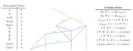
Figure 1: Example of a simple signal machine. Meta-signals are given on the left and collision rules are listed on the right side.

The input of a signal machine is defined by its initial configuration ($c_{0}$), and the output is represented by signals that comes out when no more collision occurs. Input of a signal machine is placed at the bottom of the time-space diagram at time zero, and the output consists of signals moving freely after all the collisions at the top of the time-space diagram.

We define a directed acyclic graph for a signal machine based on its collisions and dependencies between collisions. This directed acyclic graph consists of collisions as vertices and signals as edges, which are oriented according to their moving direction on space-time diagram. Based on directed acyclic graph of collisions, two major complexity measures are defined, 1) time, which is defined as the maximal length of a chain or collision depth, i.e. the length of the longest path, and 2) space, which is defined as the maximal number of signals in a time [2].

3 Structures

In this section, we present many technique that could be applied on signal machine structure due to the geometric nature of this model. These techniques help us propose our algorithm.

Proposition 1

(Middle) [4] Based on a simple geometric architecture, we can obtain the middle point of two stationary signals, i.e. signals with zero speeds. Figure 2 illustrates this technique.

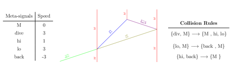
Figure 2: Geometrical technique for obtaining the middle of two stationary signals (taken from [4]).

Proposition 2

(Freezing/Unfreezing) [11]. A signal machine is able to freeze computations by replacing all the signals with a set of parallel signals during a time and then unfreeze and continue the computation, after a while.

The freezing technique is used to preserve configuration and then restore it later. During the freezing process, one freezing signal is sent from one end of the space-time diagram and it crosses all the signals. In order to perform freezing technique, for each meta-signal we define a new meta-signal representing frozen version of it. A collision between the freezing signal and a signal replaces the signal with the frozen version of it. Also, since the freezing signal may enter to a collision of some non-freezing signals, for each set of meta-signals we define a frozen version of that set, which is produced after a collision of freezing signal with a set of non-frozen signals. All the frozen signals have same velocities, so they produce parallel lines in space-time diagram and do not collide with each other. In addition, the distance between signals remain unchanged, so the configuration freezes and shifts on space [1].

To unfreeze a configuration, an unfreezing signal is sent from one end, crosses the configuration, and replaces each frozen signal by the original one (or the result of the collision, for frozen collisions). Freezing and unfreezing signals have same speeds, thus, the configuration is restored exactly as it was before, but with a shift in space.

Freezing is a useful technique and brings us a good ability in computations by signal machines. For example, when a configuration is frozen, we can consider parallel frozen signals as a set of signals, so it is possible to change their directions and even propagate the beam to everywhere and then unfreeze and retrieve the computations by an unfreezing signal with the same velocity as the freezing signal. Freezing and unfreezing procedure is depicted in Figure 3.

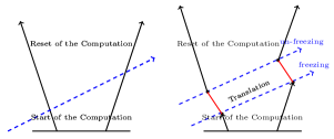
Figure 3: Freezing technique (taken from [11]).

Proposition 3

(Scaling). A signal machine can scale distances between parallel signals, and thus each computation, by a scaling factor.

The scaling means to scale down the distances between signals without any change in their velocities and rules. Thus, by scaling technique, the configuration is scaled without any change in the computation of signal machine. Scaling of parallel signals is easy by a Thales based construction. Thus, for scaling any computation (not necessarily parallel signals), we can freeze the computations to a set of parallel signals and then scale the parallel signals by a scaling signal. Finally, by a unfreezing signal which is parallel to the freezing signal, the computations with smaller scale is unfrozen and continue. In Figure 4(c), the scaling procedure and an example of applying scaling procedure on a simple signal machine (of Figure 1) is presented.

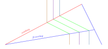
(a) Scaling parallel signals [11]

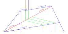
(b) Scaling any computation [11]

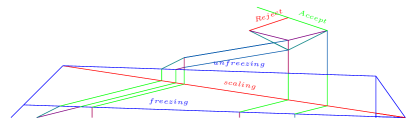
(c) Example of scaling a simple signal machine

Figure 4: Scaling.

Proposition 4

(Fractal Cloud) Applying the procedure for obtaining the middle of two signals repeatedly, a signal machine is able to halve space recursively and have a fractal-like structure which is called fractal cloud (see Figure 5).

This fractal cloud architecture is used for massively parallel computations. For example, it is possible to propagate a computation’s configuration as a beam using the fractal cloud and do computations in each branch of this fractal cloud in parallel.

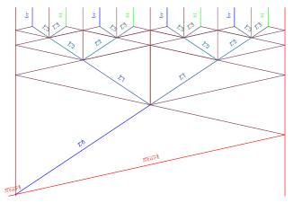
Figure 5: Division process for constructing fractal cloud (taken from [2]).

4 Nondeterministic Signal Machine

In this section, we define nondeterministic signal machine, and show that deter- ministic signal machine is capable of simulating a class of nondeterministic signal machines.

4.1 Definition

All the above mentioned signal machines are deterministic signal machines (DSM). In this paper, we introduce nondeterministic signal machine (NSM) as a signal machine which may have more than one applicable rule for a collision. Figure 6 presents a simple example of nondeterministic signal machine.
A nondeterministic signal machine is defined by a tuple $(M,S,R,c_{0})$ where:

• $M$ is a finite set of meta-signals.

• $S:M\rightarrow{\rm I\!R}$ is a function which assigns a real speed to each meta-signal.

• $R:\{\sigma_{1},\sigma_{2},...,\sigma_{n}\}\rightarrow\{\sigma_{1}^{\prime},\sigma_{2}^{\prime},...,\sigma_{p}^{\prime}\}|\{\sigma_{1}^{\prime\prime},\sigma_{2}^{\prime\prime},...,\sigma_{q}^{\prime\prime}\}|...$ is a set of collision rules which is a mapping from an arbitrary subset of $M$ with cardinality of at least two to any number of subsets of $M$, where all $\sigma_{i}$ are meta-signals of distinct speed as well as $\sigma_{j}^{\prime}$ and $\sigma_{k}^{\prime\prime}$.

• $c_{0}$ is the initial configuration.

We say that a nondeterministic signal machine accepts an input, if there exists a set of collision rules when applying on collisions, an accepting output is produced by the signal machine.

(a) meta-signals

(b) rules

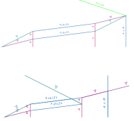
(c) two examples of possible paths for this NSM

Figure 6: A nondeterminestic signal machine with four possible diagram.

4.2 Simulation of NSM by DSM

According to definition of NSM, every deterministic signal machine is a special case of NSM. Now, we investigate if nondeterminism brings more computational power to signal machine or not.

We define k-Restricted Nondeterministic Signal Machine (k-RNSM) as a NSM having following conditions:

• No two collisions occur in exactly same time.

• At most two rules are defined for each collision.

• An input is accepted by the machine if and only if a special signal accept is produced during computation.

• If an input is accepted by the machine, at most k collision occurs before creation of the accept signal.

Theorem 4.1

Let NN be an k-RNSM, then, there exists a deterministic signal machine $D_{\textit{NN}}$ that accepts each input configuration if and only if NN accepts the input.

Proof

The idea of the proof is to produce all possible paths of nondeterministic computations of NN in a fractal cloud, and test if one of them leads to an accept signal.

Since for each input, there are at most k collisions before production of an accept signal in NN , thus, we only have to check at most $2^{k}$ different possible space-time diagrams which may be produced by NN . We produce $2^{k}$ different paths by utilizing $2^{k}$ binary unique numbers and assign them to different computation paths. Thus, computation in $D_{\textit{NN}}$ consists of two stages:

• A fractal cloud with $2^{k}$ leaves (depth of k) is produced, each leaf is used for simulation of one possible space-time diagram of NN . Thus, at the last level of the fractal cloud, in each branch or leaf we have a unique binary number and also an initial configuration of NN . To represent $2^{k}$ binary numbers we use k stationary signals. We call a set of k signals, which represent a binary number, a binary beam.

• At each leaf of fractal cloud, a possible space-time diagram of NN for the given input is simulated. In each possbile space-time diagram at most k collisions are made. According to the binary beam of a branch, for each collision, we choose between two possible collision rules and apply that.

Note that if NN accepts the input, the input signal will be produced in at least one leaf of fractal cloud in $D_{\textit{NN}}$.

4.3 constructing a fractal cloud of $2^{k}$ binary numbers and initial configuration

In order to construct $2^{k}$ binary beams, we combine the idea of decision tree and architecture of fractal cloud with k division levels [2] (see Figure 7). Also, in each dividing level of constructing fractal cloud, we use an automatically scaling procedure which is called lens device [4]. This is done in order to shrinking the data and beam according to the structure in each division.

In order to construct the cloud, we start with a initial configuration of NN and initial configuration of a fractal cloud. First, we freeze and scale the whole initial configuration of NN coupled with a beam of $\{b_{1},b_{2},...,b_{k}\}$ which is consists of k raw signals for constructing a binary number. Each signal $b_{i}$ is changed to either $0_{i}$ or $1_{i}$ at the $i$-th level. After freezing and scaling, we distribute frozen data through the fractal cloud and make a decision for signal of $b_{i}$ at $i$-th level (see Figure 7).

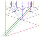
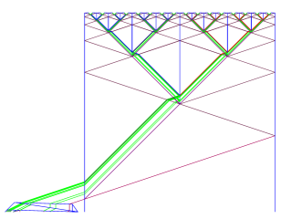
Figure 7: binary decision tree and applying it on our complete fractal cloud.

4.4 Executing one of NSM’s paths deterministically according to the binary beam

Now suppose that we are at one leaf of our constructed fractal cloud and we want to construct the corresponding space-time diagram. The idea is to simulate computations of NN collision by collision. For the $i$-th collision, we make a decision on choosing one of the at most two possible collision rules according to the value of ($b_{i}$), and apply it.

Thus, we start from the input configuration (a copy of input signals are presented in each leaf of the tree), and at the $i$-the collision, we freeze the computation and choose the collision. We suppose that the speed of freezing signal is high enough that no other collisions occurs before freezing whole the computations. A freezing signal is send toward the binary beam, and then a $message$ signal is send in opposite direction, which encodes the value of $b_{i}$. When the $message$ signal meets the encoded collision signal, according to value of message signal (True or False), one of the defined rules of NN for the current collision is applied. Also in this point, two unfreezing signals are send in both direction with same speed as the freezing signal to unfreeze the computation. Figure 8 represent how we approach in each collision point of NN.

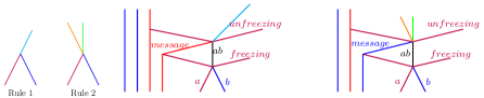
Figure 8: Execution at a collision point of a nondeterministic signal machine.

Figure 9 shows a deterministic possible path obtained by a binary beam for the NSM which is introduced in the Figure 6.

Since there are at most $k$ collisions in NN before producing the accept signal, thus, if NN accepts an input configuration, $D_{\textit{NN}}$ will produce an accept signal in at least one of its leaves of the fractal cloud. Also, if NN does not accept an input, the accept signal will not be produced in any leaves of the combinatorial comb in $D_{\textit{NN}}$. Thus, $D_{\textit{NN}}$ produces the same output as NN for any given input.

Note that the space complexity of $D_{\textit{NN}}$ for an input configuration is $O(k2^{k}s)$, where $s$ is the space complexity of NN over the input configuration.

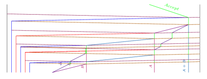
Figure 9: Executing a NSM’s path according to a binary number.

5 Conclusion and Future Works

Signal machine is a model of computation inspired by information propagation in cellular automata, where computation rules are defined according to signals and their collisions. Although many computational aspects of signal machine is previously investigated, but, the nondeterministic model of signal machines is still remained unexplored. In this paper, we introduced the concept of nondeterministic signal machine which is allowed to have more than one applicable rule for each collision. We showed that for each nondeterministic signal machine under some assumptions, there is a corresponding deterministic signal machine producing same output on any given input configuration.

As future works, we will focus on more general classes of nondeterministic signal machines. For example, we may consider the case that value $k$, maximum number of collisions before acceptance, is unknown, and check that is there a deterministic simulator for each (possibly unbounded) nondeterministic signal machine. The idea we have is that we may guess the value $k$ and check simulate a k-RNSM. If it accepts after k collisions or has at most $k-1$ collisions, we stop the simulation. Otherwise we may increase the guessed value k and repeat the simulation. Also, we will try to check that whether the restriction of having at most two nondeterministic rule for each collision reduces the computational power of NSM or not.

References

- [1] Adamatzky, A., Durand-Lose, J.: Collision-based computing. Handbook of Natural Computing pp. 1949–1978 (2012)
- [2] Duchier, D., Durand-Lose, J., Senot, M.: Fractal parallelism: Solving sat in bounded space and time. In: Algorithms and Computation, pp. 279–290. Springer (2010)
- [3] Duchier, D., Durand-Lose, J., Senot, M.: Massively parallel automata in euclidean space-time. In: Self-Adaptive and Self-Organizing Systems Workshop (SASOW), 2010 Fourth IEEE International Conference on. pp. 104–109. IEEE (2010)
- [4] Duchier, D., Durand-Lose, J., Senot, M.: Computing in the fractal cloud: modular generic solvers for sat and q-sat variants. In: Theory and Applications of Models of Computation, pp. 435–447. Springer (2012)
- [5] Durand-Lose, J.: Calculer géométriquement sur le plan-machines à signaux. Ph.D. thesis, Université Nice Sophia Antipolis (2003)
- [6] Durand-Lose, J.: Abstract geometrical computation: Turing-computing ability and undecidability. In: New Computational Paradigms, pp. 106–116. Springer (2005)
- [7] Durand-Lose, J.: Abstract geometrical computation 1: embedding black hole computations with rational numbers. Fundamenta Informaticae 74(4), 491–510 (2006)
- [8] Durand-Lose, J.: Abstract geometrical computation and the linear blum, shub and smale model. In: Computation and Logic in the Real World, pp. 238–247. Springer (2007)
- [9] Durand-Lose, J.: Abstract geometrical computation with accumulations: Beyond the blum, shub and smale model. In: 4th Conf. Computability in Europe (CiE~’08)(abstracts and extended abstracts of unpublished papers). pp. 107–116. University of Athens (2008)
- [10] Durand-Lose, J.: The signal point of view: from cellular automata to signal machines. In: JAC 2008. pp. 238–249 (2008)
- [11] Durand-Lose, J.: Abstract geometrical computation 3: Black holes for classical and analog computing. Natural computing 8(3), 455–472 (2009)