Tidal deformability of neutron and hyperon star with relativistic mean field equations of state

Abstract

We systematically study the tidal deformability for neutron and hyperon stars using relativistic mean field (RMF) equations of state (EOSs). The tidal effect plays an important role during the early part of the evolution of compact binaries. Although, the deformability associated with the EOSs has a small correction, it gives a clean gravitational wave signature in binary inspiral. These are characterized by various love numbers $k_{l}$ (l=2, 3, 4), that depend on the EOS of a star for a given mass and radius. The tidal effect of star could be efficiently measured through advanced LIGO detector from the final stages of inspiraling binary neutron star (BNS) merger.

I Introduction

The detection of gravitational waves is a major breakthrough in astrophysics/cosmology which is detected for the first time by advanced Laser Interferometer Gravitational-wave Observatory (aLIGO) detector black . Inspiraling and coalescing of binary black-hole results in emission of the gravitational waves. We may expect that in a few years the forthcoming aLIGO black , VIRGO virgo and KAGRA kagra detectors will also detect gravitational waves emitted by binary neutron star (NSs). This detection will provide a valuable guidance and a better understanding of highly compressed baryonic system. Flanagan and Hinderer flan ; tanja ; tanja1 have recently pointed out that tidal effects are also potentially measurable during the early part of the evolution when the waveform is relatively clean. It is understood that the late inspiral signal may be influenced by tidal interaction between binary stars (NS-NS), which gives the important information about the equation-of-state (EOS). The study of Refs. baio ; baio1 ; vines ; pann ; bd ; dam ; read ; vines1 ; bd1 ; fava inferred that the tidal effects could be measured using the recent generation of gravitational wave (GW) detectors.

In 1911, the famous mathematician A. E. H. Love love introduced dimensional parameter in Newtonian theory that is related to the tidal deformation of the Earth is due to the gravitational attraction between the Moon and the Sun. These Newtonian theory of tides has been imported to the general relativity dam ; pois , where it shows that the electric and magnetic type dimensionless gravitational Love number is a part of the tidal field associated with the gravito-electric and gravitomagnetic interactions. The tidal interaction in a compact binary system has been encoded in the love number and is associated with the induced deformation responded by changing shapes of the massive body. We are particularly interested for a neutron star in a close binary system, focusing on the various love number $k_{l}$ ($l$=2, 3, 4) due to the shape changes (like quadrupole, octupole and hexadecapole in the presence of an external gravitational field). Although higher love numbers ($l$=3, 4) give negligible effect, still these love numbers ($k_{l}$) can have vital importance in future gravitational wave astronomy. However, geophysicists are interested to calculate the surficial love number $h_{l}$, which describe the deformation of the body’s surface in a multipole expansion dam ; pois ; land .

We have used the equation of state from the relativistic mean filed (RMF) walecka74 ; rein89 ; ring96 and the newly developed effective field theory motivated RMF (E-RMF) furn96 ; furn97 approximation in our present calculations. Here, the degrees of freedom are nucleon, $\sigma-,$ $\omega-$, $\rho-$, $\pi-$mesons and photon. This theory very well explains the properties of finite nuclei and nuclear matter system at higher density region. Walecka has generalized walecka74 the RMF approximation and then subsequently Boguta and Bodmer boguta77 extended to the self-interaction of the $\sigma-$meson to reproduce proper experimental observables. In the E-RMF formalism, all the possible couplings of the mesons among themselves and also their cross-interaction considered furn96 ; furn97 . The self- and crossed interactions are very significant. For example, the self-interaction of $\sigma-$meson brings back the nuclear matter incompressibility $K_{\infty}$ from an unacceptable high value of $K_{\infty}\sim$600 MeV to a reasonable $K_{\infty}$ of $\sim$270 MeV boguta77 ; bodmer91 . Similarly, the quartic self-interaction of the vector meson $\omega$ soften the equation of state suga94 ; pieka05 . It is to be noted that all the mesons and their self- and cross-interaction terms in the effective Lagrangian need not to be included, because of some symmetry and their heavy masses mechl87 . This theory of dense matter fairly explains the observed massive neutron star, like PSR J1614-2230 with mass $M=1.97\pm 0.04M_{\odot}$ demo10 and PSR J0348+0432 ($M=2.01\pm 0.04M_{\odot}$) antoni13 .

The baryon octet are also introduced as the stellar system is in extra-ordinary condition such as highly asymmetric or extremely high density medium bharat07 . The coupling constants for nucleon-mesons are fitted to reproduce the properties of a finite number of nuclei, which then predict not only the observables of $\beta-$stable nuclei, but also of drip-lines and superheavy regions walecka74 ; boguta77 ; rein86 ; ring90 ; rein88 ; sharma93 ; suga94 ; lala97 . The hyperon-meson couplings are obtained from the quark model oka ; naka ; naka1 . Recently, however, the couplings are improved by taking into consideration some other properties of strange nuclear matter naka2 .

The paper is organized as follows: In Sec. II, we give a brief description on relativistic mean field (RMF/E-RMF) formalism. The ingredients of the quantum hadrodynamic model (QHD) and resulting EOSs are outlined in this section. The various tidal love numbers and tidal deformability of neutron and hyperon star are discussed in Sec. III.3,III.4 after describing the numerical scheme. Finally, the summary and concluding remarks are given in Sec. IV.

II The relativistic mean field formalism

The effective field theory motivated relativistic mean field (E-RMF) Lagrangian is designed with underlying symmetries of quantum chromodynamics (QCD) and the parameters of G1 and G2 are constructed taking into account the naive dimensional analysis and naturalness furn96 ; furn97 ; muller96 ; furn00 ; mach11 . For practical purpose, the terms in the Lagrangian are taken upto $4^{th}$ order in meson-baryon couplings. The baryon-meson interaction is given by bharat07 :

$${\cal L} = \sum_{B}\overline{\psi}_{B}\left(i\gamma^{\mu}D_{\mu}-m_{B}+g_{\sigma B}\sigma\right)\psi_{B}$$ (1)

$$+\frac{1}{2}\partial_{\mu}\sigma\partial_{\mu}\sigma-m_{\sigma}^{2}\sigma^{2}\left(\frac{1}{2}+\frac{g_{3}}{3!}\frac{g_{\sigma}\sigma}{m_{B}}+\frac{g_{4}}{4!}\frac{g_{\sigma}^{2}\sigma^{2}}{m_{B}^{2}}\right)$$

$$-\frac{1}{4}\Omega_{\mu\nu}\Omega^{\mu\nu}+\frac{1}{2}m_{\omega}^{2}\omega_{\mu}\omega^{\mu}\left(1+\eta_{1}\frac{g_{\sigma}\sigma}{m_{B}}+\frac{\eta_{2}}{2}\frac{g_{\sigma}^{2}\sigma^{2}}{m_{B}^{2}}\right)$$

$$-\frac{1}{4}R_{\mu\nu}^{a}R^{\mu\nu a}+\frac{1}{2}m_{\rho}^{2}\rho_{\mu}^{a}\rho^{a\mu}\left(1+\eta_{\rho}\frac{g_{\sigma}\sigma}{m_{B}}\right)$$

$$+\frac{1}{4!}\zeta_{0}\left(g_{\omega}\omega_{\mu}\omega^{\mu}\right)^{2}+\Lambda_{v}(g_{\rho}^{2}\rho_{\mu}^{a}\rho^{\mu a})(g_{\omega}^{2}\omega_{\mu}\omega^{\mu})$$

$$+\sum_{l}\overline{\psi}_{l}\left(i\gamma^{\mu}\partial_{\mu}-m_{l}\right)\psi_{l}.$$

The co-variant derivative $D_{\mu}$ is defined as:

$$D_{\mu}=\partial_{\mu}+ig_{\omega}\omega_{\mu}+ig_{\rho}I_{3}\tau^{a}\rho_{\mu}^{a},$$ (2)

where $R_{\mu\nu}^{a}$ and $\Omega_{\mu\nu}$ are field tensors defined as:

$$R_{\mu\nu}^{a}=\partial_{\mu}\rho_{\nu}^{a}-\partial_{\nu}\rho_{\mu}^{a}+g_{\rho}\mathcal{E}_{abc}\rho_{\mu}^{b}\rho_{\nu}^{c},$$ (3)

$$\Omega_{\mu\nu}=\partial_{\mu}\omega_{\nu}-\partial_{\nu}\omega_{\mu}.$$ (4)

Here, the symbol B stands for the baryon octet (n,p,$\Lambda$, $\Sigma^{+}$, $\Sigma^{0}$,$\Sigma^{-}$,$\Xi^{-}$,$\Xi^{0}$) and $l$ represents e^- and $\mu^{-}$. The masses $m_{B}$, $m_{\sigma}$, $m_{\omega}$, and $m_{\rho}$ are, respectively for baryons and for $\sigma$, $\omega$ and $\rho$ meson fields. In real calculation, we ignore the non-abelian term from the $\rho-$field. $I_{3}$ is the third component of isospin projection. All symbols are carrying their own usual meaning  bharat07 ; sing14 .

For a given Lagrangian density in Eq.(1), one can solve the equations of motion bharat07 ; sing14 in the mean-field level, i.e. the exchange of mesons create an uniform meson field, where the nucleon has a simple harmonic motion. Then we calculate the energy-momentum tensor within the mean field approximation (i.e. the meson fields are replaced by their classical number) and get the EOS as a function of baryon density. The EOS remains uncertain at density larger than the saturation density of nuclear matter, $\rho_{n}\sim$3 $\times$ 10¹⁴ g cm^-3. At these densities, neutrons can no longer be considered, which may consists mainly of heavy baryons (mass greater than nucleon) and several other species of particles expected to appear due to the rapid rise of the baryon chemical potentials baldo . The $\beta$-equilibrium and charge neutrality are two important conditions for the neutron/hyperon rich-matter. Both these conditions force the stars to have $\sim$90$\%$ of neutron and $\sim$10$\%$ proton. With the inclusion of baryons, the $\beta-$equilibrium conditions between chemical potentials for different particles:

$$\mu_{p}=\mu_{\Sigma^{+}}=\mu_{n}-\mu_{e},$$

$$\mu_{n}=\mu_{\Sigma^{0}}=\mu_{\Xi^{0}}=\mu_{n},$$

$$\mu_{\Sigma^{-}}=\mu_{\Xi^{-}}=\mu_{n}+\mu_{e},$$

$$\mu_{\mu}=\mu_{e},$$

and the charge neutrality condition is satisfy by

$$n_{p}+n_{\Sigma^{+}}=n_{e}+n_{\mu^{-}}+n_{\Sigma^{-}}+n_{\Xi^{-}}.$$ (6)

The corresponding pressure and energy density of the charge neutral beta-equilibrated neutron star matter (which includes the lowest lying octet of baryons) is then given by bharat07 :

$$\mathcal{E} = \sum_{B}\frac{2}{(2\pi)^{3}}\int_{0}^{k_{B}}d^{3}kE_{B}^{*}(k)+\frac{1}{8}\zeta_{0}g_{\omega}^{2}\omega_{0}^{4}$$ (7)

$$+m_{\sigma}^{2}\sigma_{0}^{2}\left(\frac{1}{2}+\frac{g_{3}}{3!}\frac{g_{\sigma}\sigma_{0}}{m_{B}}+\frac{g_{4}}{4!}\frac{g_{\sigma}^{2}\sigma_{0}^{2}}{m_{B}^{2}}\right)$$

$$+\frac{1}{2}m_{\omega}^{2}\omega_{0}^{2}\left(1+\eta_{1}\frac{g_{\sigma}\sigma_{0}}{m_{B}}+\frac{\eta_{2}}{2}\frac{g_{\sigma}^{2}\sigma_{0}^{2}}{m_{B}^{2}}\right)$$

$$+\frac{1}{2}m_{\rho}^{2}\rho_{03}^{2}\left(1+\eta_{\rho}+\frac{g_{\sigma}\sigma_{0}}{m_{B}}\right)+3\Lambda_{v}(g_{\rho}\rho_{03})^{2}(g_{\omega}\omega_{0})^{2}$$

$$+\sum_{l}\mathcal{E}_{l},$$

and

$$P = \sum_{B}\frac{2}{3(2\pi)^{3}}\int_{0}^{k_{B}}d^{3}k\frac{k^{2}}{E_{B}^{*}(k)}+\frac{1}{8}\zeta_{0}g_{\omega}^{2}\omega_{0}^{4}$$ (8)

$$-m_{\sigma}^{2}\sigma_{0}^{2}\left(\frac{1}{2}+\frac{g_{3}}{3!}\frac{g_{\sigma}\sigma_{0}}{m_{B}}+\frac{g_{4}}{4!}\frac{g_{\sigma}^{2}\sigma_{0}^{2}}{m_{B}^{2}}\right)$$

$$+\frac{1}{2}m_{\omega}^{2}\omega_{0}^{2}\left(1+\eta_{1}\frac{g_{\sigma}\sigma_{0}}{m_{B}}+\frac{\eta_{2}}{2}\frac{g_{\sigma}^{2}\sigma_{0}^{2}}{m_{B}^{2}}\right)$$

$$+\frac{1}{2}m_{\rho}^{2}\rho_{03}^{2}\left(1+\eta_{\rho}\frac{g_{\sigma}\sigma_{0}}{m_{B}}\right)+\Lambda_{v}(g_{\rho}\rho_{03})^{2}(g_{\omega}\omega_{0})^{2}$$

$$+\sum_{l}P_{l},$$

where $P_{l}$ and $\mathcal{E}_{l}$ are lepton’s pressure and energy density, respectively. $E_{B}^{*}=(k_{B}^{2}+M_{B}^{*2})^{1/2}$ is the effective energy, $k_{B}$ is the Fermi momentum of the baryons. $M_{p}^{*}$ and $M_{n}^{*}$ are the proton and neutron effective masses written as

$$M_{p}^{*}=M_{p}-g_{\sigma}\sigma_{0}$$ (9)

and

$$M_{n}^{*}=M_{n}-g_{\sigma}\sigma_{0}.$$ (10)

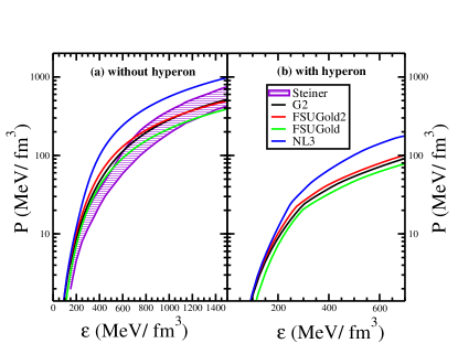
Figure 1: (Color online) The equations of state obtained for nuclear and hyper-nuclear matter under charge neutrality as well as the $\beta-$ equilibrium condition for G2 furn97 , FSUGold2 fsu2 , FSUGold pieka05 and NL3 lala97 force parameters are compared with the empirical data ste10 (shaded area in the graph)for r_ph=R with the uncertainty of $2\sigma$. Here, R and r_ph are the neutron radius and the photospheric radius, respectively.

III Results and Discussions:

III.1 Equations of state

In this section, we present the results of our calculations in Figs. 1-9 and Table 2. Before going to the estimation of the tidal deformibility parameter $\lambda$, we check the validity of the EOSs obtained with various force parameters. Fig.1 displays the equation of state for G2 furn97 , FSUGold2 fsu2 , FSUGold pieka05 and NL3 lala97 parameter sets. From the left panel of Fig. 1(a), it is obvious that all the EOSs follow similar trend. Among these four, the celebrity NL3 set gives the stiffest EOS and the relatively new FSUGold represents the softer character. This is because of the large and positive $g_{4}$ value as well as the introduction of isoscalar-isovector coupling ($\Lambda$) in the FSUGold set pieka05 . To have an understanding on the softer and stiffer EOSs by various parametrizations, we compared their coupling constants and other parameters of the sets in Table 1. We notice a large variation in their effective masses, incompressibilities and other nuclear matter properties at saturation. For higher energy density $\mathcal{E}\sim 500-1400$ MeV fm^-3, except NL3 set, which has the lowest nucleon effective mass, all other sets are found in the region of empirical data with the uncertainty of 2$\sigma$ ste10 .

Fig. 1(b) shows a hump type structure on the nucleon-hyperon equation of state at $\mathcal{E}$ around 400-500 MeV fm^-3. This kink ($\mathcal{E}\sim$ 200-300 MeV) shows the presence of hyperons in the dense system. Here, the repulsive component of the vector potential becomes more important than the attractive part of the scalar interaction. As a result the coupling of the hyperon-nucleon strength gets weak. At a given baryon density, the inclusion of hyperons lower significantly the pressure compared to the equation of state of having without hyperons. This is possible due to the higher energy of the hyperons, as the neutrons are replaced by the low-energy hyperons. The hyperon couplings are expressed as the ratio of the meson-hyperon and meson-nucleon couplings:

$$\chi_{\sigma}=\frac{g_{Y\sigma}}{g_{N\sigma}},\chi_{\omega}=\frac{g_{Y\omega}}{g_{N\omega}},\chi_{\rho}=\frac{g_{Y\rho}}{g_{N\rho}}.$$ (11)

In the present calculations, we have taken $\chi_{\sigma}$ = 0.7 and $\chi_{\omega}=\chi_{\rho}$ = 0.783. One can find similar calculations for stellar mass in Refs. glen20 ; mene ; weis12 ; lope14 .

Table 1: Parameters and saturation properties for NL3 lala97 , G2 furn97 , FSUGold pieka05 , and FSUGold2 fsu2 . The parameters $g_{\sigma}$, $g_{\omega}$, $g_{\rho}$, $g_{3}$, and $g_{4}$ are calculated from nuclear matter the given saturation properties using the relations suggested by the authors of Ref. glen20 .

Parameters	NL3	G2	FSUGold	FSUGold2
$m_{n}$(MeV)	939	939	939	939
$m_{\sigma}$(MeV)	508.194	520.206	491.5	497.479
$m_{\omega}$(MeV)	782.501	782	783	782.5
$m_{\rho}$(MeV)	763	770	763	763
$g_{\sigma}$	10.1756	10.5088	10.5924	10.3968
$g_{\omega}$	12.7885	12.7864	14.3020	13.5568
$g_{\rho}$	8.9849	9.5108	11.7673	8.970
$g_{3}$(MeV)	1.4841	3.2376	0.6194	1.2315
$g_{4}$	-5.6596	0.6939	9.7466	-0.2052
$\eta_{1}$	0	0.65	0	0
$\eta_{2}$	0	0.11	0	0
$\eta_{\rho}$	0	0.390	0	0
$\zeta_{0}$	0	2.642	12.273	4.705
$\Lambda$	0	0	0.03	0.000823
$\rho_{0}$(fm${}^{-3})$	0.148	0.153	0.148	0.1505$\pm$0.00078
E/A(MeV)	-16.299	-16.07	-16.3	-16.28$\pm$0.02
K∞(MeV)	271.76	215	230	238.0$\pm$ 2.8
J(MeV)	37.4	36.4	32.59	37.62$\pm$1.11
L(MeV)	118.2	101.2	60.5	112.8$\pm$ 16.1
$m_{n}^{*}$/$m_{n}$	0.6	0.664	0.610	0.593$\pm$0.004

III.2 Mass and radius of neutron star

Once the equations of state for various relativistic forces are fixed, then we extend our study for the evaluation of the mass and radius of the isolated neutron star. The Tolmann-Oppenheimer-Volkov (TOV) equations tolm39 have to be solved for this purpose, where EOSs are the inputs. The TOV equations are written as:

$$\frac{dP(r)}{dr}=-\frac{[{\mathcal{E}}(r)+P(r)][M(r)+{4\pi r^{3}P(r)}]}{r^{2}(1-\frac{2M(r)}{r})},$$ (12)

and

$$\frac{dM(r)}{dr}={4\pi r^{2}{\mathcal{E}}(r)}.$$ (13)

For a given EOS, the Tolmann-Oppenheimer-Volkov (TOV) equations tolm39 must be integrated from the boundary conditions $P(0)=P_{c}$, and $M(0)$=0, where $P_{c}$ and M(0) are the pressure and mass of the star at $r$=0 and the value of $r$(= $R$), where the pressure vanish defines the surface of the star. Thus, at each central density we can uniquely determine a mass $M$ and a radius R of the static neutron and hyperon satrs using the four chosen EOSs. The estimated result for the maximum mass as a function of radius are compared with the highly precise measurements of two massive ($\sim 2M_{\odot}$) neutron star demo10 ; antoni13 and extraction of stellar radii from X-ray observation ste10 , are shown in Figs. 2(a) and 2 (b) . From recent observations demo10 ; antoni13 , it is clearly illustrated that the maximum mass predicted by any theoretical models should reach the limit $\sim 2.0M_{\odot}$, which is consistent with our present prediction from the G2 equation of state of nucleonic matter compact star with mass 1.99$M_{\odot}$ and radius 11.25 km. From X-ray observation, Steiner et. al. ste10 predicted that the most-probable neutron star radii lie in the range 11-12 km with neutron star masses$\sim$1.4$M_{\odot}$ and predicted the EOS is relatively soft in the density range 1-3 times the nuclear saturation density. As explained to earlier, stiff EOS like NL3 predicts larger stellar radius 13.23 km and a maximum mass 2.81 $M_{\odot}$. Though FSUGold and FSUGold2 are from the same RMF model with similar terms in the Lagrangian, their results for neutron star are quite different with FSUGold2 suggesting a larger and heavier NS with mass 2.12$M_{\odot}$ and radius 12.12 km compare to mass and radius (1.75$M_{\odot}$ and 10.76 km) of the FSUGold. Because in FSUGold2 EOS at high densities, the impact comes from the quartic vector coupling constant $\zeta_{0}$ and also the large value of the slope parameter L=112.8 $\pm$16.1 MeV (see Table 1) tend to predict the neutron star with large radius horo01 . From the observational point of view, there are large uncertainties in the determination of the radius of the star rute ; gend ; cott , which is a hindrance to get a precise knowledge on the composition of the star atmosphere. One can see that G2 parameter is able to reproduce the recent observation of 2.0$M_{\odot}$ NS. But the presence of hyperon matter under $\beta$-equilibrium soften the EOS, because they are more massive than nucleons and when they start to fill their Fermi sea slowly replacing the highest energy nucleons. Hence, the maximum mass of NS is reduced by $\sim$0.5 unit solar mass due to the high baryon density. For example, the stiffer NL3 equation of state gives the maximum NS mass $\sim$2.81$M_{\odot}$ and the presence of hyperon-matter reduces the mass to $\sim$2.25$M_{\odot}$ as shown in Fig. 2(b).

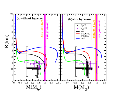
Figure 2: (Color online) The mass-radius profile for the force parameters like G2 furn97 , FSUGold2 fsu2 , FSUGold pieka05 and NL3 lala97 used. The solid circles($r_{ph}$=R) and triangles($r\gg$R) are represent the observational constraints ste10 , where $r_{ph}$ is the photospheric radius. The verticle sheded region correspond to the recent observation demo10 ; antoni13 .

These results give us warning that most of the present sets of hyperon couplings unable to reproduce the recently observed mass of neutron star like PSR J1614-2230 with mass $M=1.97\pm 0.04M_{\odot}$ demo10 and the PSR J0348+0432 with $M=2.01\pm 0.04M_{\odot}$ antoni13 . Probably, this suggest us to modify the coupling constants and get the equations of state proper, so that one can explain all the mass-radius observation till date. Further, one can see that in Fig. 2(b) mass-radius curve of G2, FSUGold, FSUGold2 with hyperon lies in the range of predicted equation of state between the $r_{ph}$=R and $r_{ph}\gg$R cases is the high density behaviour ste10 .

III.3 Various tidal love number of compact star

When spherical star placed in a static external quadrupolar tidal field $\mathcal{E}_{ij}$ then the star will be deformed and quadrupole deformation will be the leading order perturbation. Such a deformation is defined as the ratio of the mass quadrupole moment of a star Q_ij to the external tidal field $\mathcal{E}_{ij}$:

$$\lambda=-\frac{Q_{ij}}{\mathcal{E}_{ij}}.$$ (14)

Specifically, the observable of the tidal deformability parameter $\lambda$ depends on the EOS via both the neutron star (NS) radius and a dimensionless quantity k₂, called the Love number and is given by the relation:

$$\lambda=\frac{2}{3}k_{2}R^{5},$$ (15)

and the dimensionless tidal-deformability($\Lambda$) is related with the compactness parameter $C=M/R$ as:

$$\Lambda=\frac{2k_{2}}{3C^{5}},$$ (16)

where R is the radius of the (spherical) star in isolation. Now, we have to get k₂ for the calculation of the deformability parameter $\lambda$, which is the key quantity of deformation due to the gravitational attraction of the binary stars with each other. This force of attraction becomes more and more important in the course of time, because of the reduction of the orbital distance between them. The orbital distance between the binary decreases as the companion star emits gravitational radiation. As a result, the binary accelerates and finally merge with each other and possibly turns to a black hole. Thus, the estimation of the leading order quadrupole electric tidal love number $k_{2}$ along with other higher order love numbers $k_{3}$ and $k_{4}$ are very important for the detection of gravitational wave.

To estimate the love numbers $k_{l}$ ($l$=2, 3, 4), along with the evaluation of the TOV equations, we have to compute $y=y_{l}(R)$ with initial boundary condition $y(0)=l$ from the following first order differential equation iteratively tanja ; tanja1 ; thib1 ; pois :

$$r\frac{dy(r)}{dr}+y(r)^{2}+y(r)F(r)+r^{2}Q(r)=0,$$ (17)

with,

$$F(r)=\frac{r-4\pi r^{3}[{\mathcal{E}}(r)-P(r)]}{r-2M(r)},$$ (18)

$$Q(r)=\frac{4\pi r(5{\mathcal{E}}(r)+9P(r)+\frac{{\mathcal{E}}(r)+P(r)}{{\partial P(r)}/{\partial{\mathcal{E}}(r)}}-\frac{l(l+1)}{4\pi r^{2}})}{r-2M(r)}$$

$$-4\Big{[}\frac{M(r)+4\pi r^{3}P(r)}{r^{2}(1-2M(r)/r)}\Big{]}^{2}.$$ (19)

Once, we know the value of $y=y_{l}(R)$, the electric tidal love numbers $k_{l}$ are found from the following expression thib1 :

$$k_{2}=\frac{8}{5}(1-2C)^{2}C^{5}[2C(y_{2}-1)-y_{2}+2]\Big{\{}2C(4(y_{2}+1)C^{4}+(6y_{2}-4)C^{3}+$$

$$(26-22y_{2})C^{2}+3(5y_{2}-8)C-3y_{2}+6)-3(1-2C)^{2}(2C(y_{2}-1)-y_{2}+2)log\Big{(}\frac{1}{1-2C}\Big{)}\Big{\}}^{-1},$$ (20)

$$k_{3}=\frac{8}{7}(1-2C)^{2}C^{7}[2(y_{3}-1)C^{2}-3(y_{3}-2)C+y_{3}-3]\Big{\{}2C[4(y_{3}+1)C^{5}+2(9y_{3}-2)C^{4}$$

$$-20(7y_{3}-9)C^{3}+5(37y_{3}-72)C^{2}-45(2y_{3}-5)C+15(y_{3}-3)]-15(1-2C)^{2}$$

$$(2(y_{3}-1)C^{2}-3(y_{3}-2)C+y_{3}-3)log\Big{(}\frac{1}{1-2C}\Big{)}\Big{\}}^{-1},$$ (21)

and

$$k_{4}=\frac{32}{147}(1-2C)^{2}C^{9}[12(y_{4}-1)C^{3}-34(y_{4}-2)C^{2}+28(y_{4}-3)C-7(y_{4}-4)]\Big{\{}2C[8(y_{4}+1)C^{6}$$

$$+(68y_{4}-8)C^{5}+(1284-996y_{4})C^{4}+40(55y_{4}-116)C^{3}+(5360-1910y_{4})C^{2}+105(7y_{4}-24)C-105(y_{4}-4)]$$

$$-15(1-2C)^{2}[12(y_{4}-1)C^{3}-34(y_{4}-2)C^{2}+28(y_{4}-3)C-7(y_{4}-4)]log\Big{(}\frac{1}{1-2C}\Big{)}\Big{\}}^{-1},$$ (22)

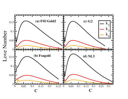
Figure 3: (Color online)The tidal love numbers $k_{2},k_{3},k_{4}$ as a function of the mass of the four selected EOSs of the neutron star.

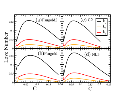
Figure 4: (Color online) Same as Fig. 3 but for hyperon star.

As we have emphasized earlier, the dimensionless love number $k_{l}$ (l=2, 3, 4) is an important quantity to measure the internal structure of the constituent body. These quantities directly enter into the gravitational wave phase of inspiralling binary neutron star (BNS) and extract the information of the EOS. Notice that equations (20)-(22) contain an overall factor $(1-2C)^{2}$, which tends to zero when the compactness approaches the compactness of the black hole, i.e. $C^{BH}$=1/2 thib . Also, it is to be pointed out that the presence of multiplication order factor $C$ with $(1-2C)^{2}$ in the expression of $k_{l}$ that the value of the love number of a black hole simply becomes zero, i.e. $k^{BH}_{l}$=0.

Table 2: Properties of a 1.4$M_{\odot}$ neutron and hyperon star for different class of the EOS. The quadrupolar tidal polarizability $\lambda$ and uncertainty error $\Delta\tilde{\lambda}$ in (10³⁶g cm² s²).

Neutron Star
EOS	$R(km)$	$C$	$f_{c}$(Hz)	$k_{2}$	$k_{3}$	$k_{4}$	$h_{2}$	$h_{3}$	$h_{4}$	$\lambda$	$\Delta\tilde{\lambda}$	$\Lambda$
NL3	14.422	0.144	1256.7	0.1197	0.0353	0.0142	0.9775	0.6519	0.5074	7.466	2.027	1288.81
G2	13.148	0.157	1440.9	0.0934	0.0265	0.0103	0.8879	0.5951	0.4596	3.668	1.486	652.76
FSUGold2	13.850	0.149	1332.4	0.1040	0.0301	0.0119	0.9275	0.6237	0.4854	5.299	1.763	944.08
FSUGold	12.236	0.170	1608.0	0.0882	0.0244	0.0071	0.8589	0.5634	0.4268	2.418	1.178	414.13
Hyperon Star
NL3	14.430	0.143	1252.9	0.1203	0.0355	0.0143	0.9800	0.6541	0.5096	7.527	2.018	1341.20
G2	12.686	0.163	1520.6	0.0804	0.0229	0.0088	0.8434	0.5707	0.4399	2.641	1.321	465.83
FSUGold2	13.690	0.151	1355.9	0.0988	0.0287	0.0113	0.9108	0.6154	0.4789	4.750	1.696	839.04
(FSUGold)${}_{1.3M_{\odot}}$	9.922	0.194	2119.0	0.0421	0.0116	0.0042	0.6884	0.4683	0.3518	0.4048	0.530	102.14

Fig. 3 shows the tidal love numbers $k_{l}$ ($l$=2, 3, 4) as a function compactness parameter $C$ for the neutron star with four selected EOSs. The result of $k_{l}$ suddenly deceases with increasing compactness (C = 0.06-0.25). For each EOS, the value of $k_{2}$ appears to be a maximum between $C=0.06-0.07$. However, we are mainly interested in the neutron star masses at $\sim$1.4$M_{\odot}$. Because of the tidal interactions in the neutron star binary, the shape of the star acquires quadrupole, octupole, hexadecapole and other higher order deformations. The value of the love numbers for corresponding shapes are shown in Table 2. The values of $k_{l}$ decreases gradually with increase of multi-pole moments. Thus, the quadrupole deformibility has the maximum effects on the binary star merger. Similarly, in Fig. 4, the dimensionless love number $k_{l}$ is shown as a function of compactness for the hyperon star. With the inclusion of hyperons, the effect of the core is negligible due to the softness of the EOSs. The values of $k_{l}$ is different for a typical neutron-hyperon star with 1.4 $M_{\odot}$ for various sets are listed in the lower portion of Table 2. The radius and respective mass-radius ratio is also given in the Table 2. The table also reflects that the love numbers decrease slightly or remains unchanged with the addition of hyperon in the neutron star. The neutron star surface or solid crust is not responsible for any tidal effects, but instead it is the matter mainly in the outer core that gives the largest contribution to the tidal love numbers. It is relatively unaffected by changing the composition of the core and leave it at that. Thus instigate the calculation for the surficial love number $h_{l}$ for both neutron and hyperon star binary.

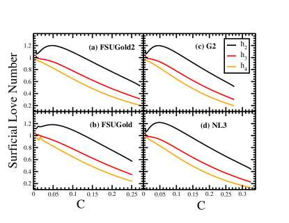
Figure 5: (Color online) Surficial love number h_l as a function of compactness C of a neutron star, for selected values of $l$.

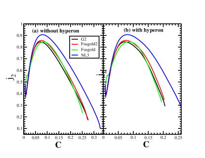
Figure 6: (Color online) The magnetic tidal love number for selected EOSs.

Next, we calculate the surficial love number $h_{l}$ which describes the deformation of the body’s surface in a multipole expansion. Recently, Damour and Nagar thib have given the surficial love number (also known as shape love number) $h_{l}$ for the coordinate displacement $\delta R$ of the body’s surface under the external tidal force. Alternatively, Landry and Poisson land have proposed the defination of Newtonian love number in terms of a curvature perturbation $\delta\mathcal{R}$ instead of a surface displacement $\delta R$. For a perfect fluid, the relation between the surficial love number $h_{l}$ and tidal love number $k_{l}$ is given as

$$h_{l}=\Gamma_{1}+2\Gamma_{2}k_{l}$$ (23)

$$\Gamma_{1}=\frac{l+1}{l-1}(1-C)F(-l,-l,-2l;2C)$$

$$-\frac{2}{l-1}F(-l,-l-1,-2l;2C),$$

$$\Gamma_{2}=\frac{l}{l+2}(1-C)F(l+1,l+1,2l+2;2C)$$

$$+\frac{2}{l+2}F(l+1,l,2l+2;2C).$$ (24)

where F(a,b,c;z) is the hypergeometric function. Fig. 5 shows the results of surficial love number $h_{l}$ of a neutron star as a function of compactness parameter C. Unlike the initially increasing and then decreasing trend of the tidal love number $k_{l}$, the surficial love number $h_{l}$ decreases almost exponentially with the compactness parameter. At the minimum value of the compactness parameter, the maximum value of the shape love number of each multipole moment approaches 1. Thus, we zero in on to the Newtonian relation i.e $h_{l}=1+2k_{l}$. Again one can compute from Table 2 that the surficial love number $h_{l}$ decreases $\sim 20\%$ from one moment to another. For example, $h_{2}=0.9775$ and $h_{3}=0.6519$ and $h_{4}=0.5074$ for NL3 parameter sets.

Furthermore, we also calculate the ”magnetic” tidal love number $j_{l}$. Here, we give only the quadrupolar case ($l=2$), which is expressed as:

$$j_{2}=\Big{\{}96C^{5}(2C-1)(y_{2}-3)\Big{\}}\Big{\{}5(2C(12(y_{2}+1)C^{4}$$

$$+2(y_{2}-3)C^{3}+2(y_{2}-3)C^{2}+3(y_{2}-3)C-3y_{2}+9)$$

$$+3(2C-1)(y_{2}-3)log(1-2C))\Big{\}}^{-1}.$$ (25)

After inserting the value of $y_{2}$ in eq. (25), we compute the magnetic tidal love number $j_{2}$ in a hydrostatic equilibrium condition for a non-rotating neutron star. This gives important information about the internal structure pois without changing the tidal love number $k_{2}$. At $C$=0.01, the magnetic love number $j_{2}$ is nearly 0.4. In both cases (with and without hyperons), $j_{2}$ is maximum within the compactness 0.06 to 0.07 for all the four EOSs (See Fig. 6). Then the value of $j_{2}$ the decreases sharply with increase of compactness. The NL3 parameter set gives a maximum $j_{2}$ in both the systems, while rest of the three sets predict comparable $j_{2}$.

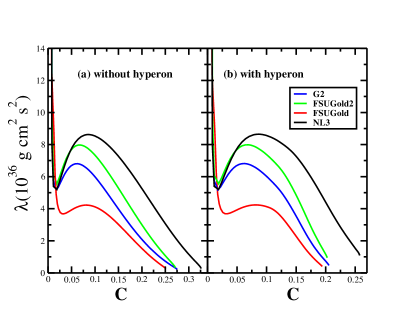
Figure 7: (Color online) The tidal deformability $\lambda$ as a function of the compactness $C$ for the four EOS with and without hyperon.

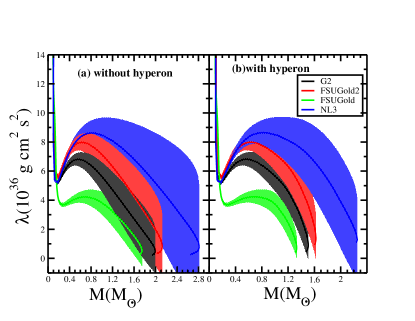
Figure 8: (Color online) Tidal deformability $\lambda$ of a single neutron star as a function of the neutron-star mass for a range of EOSs. The estimate of uncertainties in measuring $\lambda$ for equal mass binaries at a distance of D = 100 Mpc is shown for the Advanced LIGO detector in shaded area. (b) Same as (a), but for hyperon star.

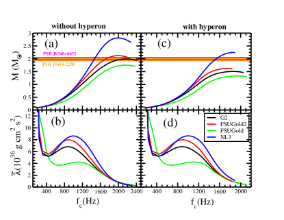
Figure 9: (Color online)(a,c) The mass-cut-off frequency f_c profile of normal and hyperon star using four EOS. (b) The tidal deformabilty with cut-off frequency plot of the neutron star(d) Same as (b), but for hyperon star.

III.4 Tidal deformability and cut-off frequency of compact star

From equation (15), it is known that the tidal deformability $\lambda$ is a function of the linear tidal love number $k_{2}$ and the fifth power of the radius $R^{5}$ of the compact star. For this purpose, we solve numerically Eqns.(12-20) using the initial boundary condition. To examine the results of tidal deformability with and without hyperons, we have shown the $\lambda-C$ plot in Fig. 7, where we have considered a single neutron star under the influence of an external tidal field with adiabatic approximation using the four equations of state. In this case, the orbital evaluation time scale is much larger than the time scale needed to assume the star as a stationary configuration. From the very beginning, we mark an infinitely large $\lambda$ corresponding to a small compactness i.e. $C\sim$0.02. Further, the $\lambda$ value falls to a minima that rises again resulting in a hump like pattern for each EOS. It is noteworthy that in Fig. 7(b) by introducing the NL3 case with hyperon, there is remarkable but mere deviation in $\lambda$ value i.e 7.527 g cm² s² ( without hyperon $\lambda$= 7.466 g cm² s²). Since, the tidal deformability $\lambda$ is a surface phenomenon, it is very much getting affected by the radius of the star in both normal neutron star and hyperon star. Thus, the tidal deformability $\lambda$ becomes highly sensitive on the radius $R$ even though $k_{2}$ is small. We estimate the radii to be within 12.236$-$14.422 km for a neutron star of mass 1.4$M_{\odot}$ and the range is 13.690$-$14.430 km for neutron-hyperon star for all the four stiff or soft equations of state (see Table 2).

Fig. 8, shows the tidal deformability for both neutron and hyperon stars. We have a large radii for a smaller stellar mass of $\sim 0.1M_{\odot}$ in both cases. At this value of mass and radius, the tidal deformability $\lambda$ becomes maximum, because for a large radius with smaller mass, the force of attraction within the star is weak and when another star comes closure, the gravitational pull over ride maximum at the surface part of the star. This phenomena is true for both neutron as well as hyperon stars tanja ; tanja1 . Then, suddenly the tidal deformibility decreases and again increases as shown in the figure making a broad peak at around M=0.7$-$0.8$M_{\odot}$ and then decrease smoothly with increase the mass of the star. Since, the tidal deformibility depends a lot on both mass and radius of a neutron star, it is imperative to measure the radius of the star precisely, as the mass is already measured with very good precession. Recently, Steiner et.al., predicted the most extreme limit for the tidal deformabilities between 0.6 and 6 $\times$ 10³⁶ g cm² s² for 1.4$M_{\odot}$ with 95$\%$ confidence. This range can be constraint on high dense matter of any measurements ste15 . Mostly, the binaries masses are about 1.4$M_{\odot}$, so in particular we are interested to study the phenomena within this mass range and the results are summarize in Table 2. Comparing the results, we notice that the tidal deformability $\lambda$ is quite sensitive to the EOS. It is more for stiffer EOS, because of the high-density behavior of the symmetry energy fattev .

Finally, we calculate the weighted tidal deformability of the binary neutron star of mass $m_{1}$ and $m_{2}$ and is approximate is tanja ; tanja1 :

$$\tilde{\lambda}=\frac{1}{26}\left[\frac{m_{1}+12m_{2}}{m_{1}}\lambda_{1}+\frac{m_{2}+12m_{1}}{m_{2}}\lambda_{2}\right],$$ (26)

and the root mean square (rms) measurement uncertainty $\Delta\tilde{\lambda}$ can be calculated following approximate formula tanja ; tanja1 :

$$\Delta\tilde{\lambda}\approx\alpha\left(\frac{M}{M_{\odot}}\right)^{2.5}\left(\frac{m_{2}}{m_{1}}\right)^{0.1}\left(\frac{f_{cut}}{Hz}\right)^{-2.2}\left(\frac{D}{100Mpc}\right),$$ (27)

where $\alpha$ = 1.0 $\times$ 10⁴² g cm² s² is the tidal deformability for a single Advanced LIGO detector and $f_{cut}$ ($f_{end}$) cutoff frequency dam for the end stage of the inspiral binary neutron stars. D denotes the luminosity distance from the source to observer.

The weighted tidal deformibility for neutron and hyperon stars and their corresponding masses as cut-off frequency $f_{cut}$ is shown in Fig. 9. The cut-off frequency is a stopping criterion to estimate when the tidal model no longer describes the binary. Here, we take the cut-off to be approximately when the two neutron stars come into contact, estimated as in Eq.36 of Ref. dam . Specifically, we use $f_{cut}=2f_{orb.}^{N(R_{1}+R_{2})}$, where $f_{orb.}^{N(R_{1}+R_{2})}$ is the Newtonian orbital frequency corresponding to the orbital separation where two unperturbed neutron stars with radii $R_{1}$ and $R_{2}$ would touch. In the upper panel Fig. 9(a,c), it shows the variation of mass of the binary as a function of cut-off frequency $f_{cut}$. Here, we considered $m_{1}=m_{2}$, i.e., both the masses of the binary are equal. Initially, the masses of the stars 0.2 $M_{\odot}$ remain almost constant upto $f_{cut}\approx 400$ Hz. Then the mass increases nearly exponentially upto a maximum mass of $\approx$1.75$-$2.81$M_{\odot}$ (for NS) and $\approx$1.33$-$2.25$M_{\odot}$ (for hyperon star) and then decreases. By this time, the cut-off frequency $f_{cut}$ attains quite large value. When the individual mass of the binary is 1.4$M_{\odot}$, the NL3 set weighted tidal deformibility achieve the cut-off frequency $f_{cut}\approx 1256.7$ Hz is the minimum contrary to the $f_{cut}\approx 1608.0$ Hz of FSUGold at the same mass of the single NS. It is also clear from the figure that the weighted tidal deformability of the NS for the four models are 7.466, 3.668, 5.229 and 2.418 for NL3, G2, FSUGold2 and FSUGold, respectively with the corresponding frequency 1256.7, 1440.9, 1332.4 and 1608.0 Hz.

Using the cut-off frequency, we calculate the uncertainty in the measurement of the tidal deformability ($\Delta\tilde{\lambda}$) obtained from these four EOSs for an equal-mass binary star inspiral at 100 Mpc from aLIGO detector (shaded region in Fig. 8). The uncertainty in the lower mass region (0.4$-$1.0$M_{\odot}$) of the NS $\Delta\tilde{\lambda}$ is smaller. Similar results are found in the case of hyperon star also. Interestingly, the error ($\Delta\tilde{\lambda}$) increases with increase the mass of the binary for all the EOSs. From Table 2, by comparing the $\Delta\tilde{\lambda}$ obtained from all the EOSs, we find that predicted errors are greater than the measured value for a star of mass 1.4$M_{\odot}$.

IV Summary and Conclusions

In summary, four different models have been extensively applied which are obtained from effective field theory motivated relativistic mean field formalism. This effective interaction model satisfies the nuclear saturation properties and reproduce the bulk properties of finite nuclei with a very good accuracy. We used these four forces of interaction and calculate the equations of state for neutron and hyperon stars matter. It is noteworthy that each term of the interaction has its own meaning and has specific character. The inclusion of extra terms (nucleons replaced by baryons octet) in the Lagrangian contribute to soften the EOS and the matter becomes less compressible. Hence, there is decrease in the maximum mass by $\sim 0.5M_{\odot}$ than the pure neutron star.

We have extended our calculations to various tidal responses both for electric-type (even-parity) and magnetic-type (odd-parity) of neutron and hyperon stars in the influence of an external gravitational tidal field. The love numbers are directly connected with surficial love number $h_{l}$ associated with the surface properties of the stars. Subsequently, we study the quadrupolar tidal deformability $\lambda$ of normal neutron star and hyperon star using different set of equations of state. These tidal deformabilities particularly depend on the quadrupole love number $k_{2}$ and radius ($R$) of the isolated star. Although the maximum value of $k_{2}$ is not very sensitive to the EOS for neutron and hyperon stars lying in the range $k_{2}\approx 0.144-0.170$ and $0.143-0.194$ for neutron and hyperon stars, respectively, but it is very much sensitive to the radius of the star.

We find that aLIGO can constraint on the existence of hyperon star, i.e., the inner core of the NS has hyperons, but detecting them can be much harder. However, it should be able to constraint the neutron star deformability to $\lambda\leq$10 $\times$ 10³⁶ g cm² s² for a binary of 1.4$M_{\odot}$ neutron stars at a distance 100 Mpc from the detector. Also, the present calculations suggest to use the portion of the signal with the gravitational wave frequency less than 400 Hz. In future, we expect that aLIGO should be able to measure $\lambda$ even for neutron stars masses up to 2.0$M_{\odot}$ and consequently constraint the stiffness of the equations of state.

ACKNOWLEDGEMENTS:

Bharat Kumar would like to take this oppertunity to convey special thanks Tanja Hinderer whose keen interest, fruitful discussions and useful suggestions.

References

- (1) B. P. Abbott et. al., Phys. Rev. Lett. 116, 061102 (2016) ;“LIGO,” www.ligo.caltech.edu.
- (2) “VIRGO,” www.virgo.infn.it.
- (3) “Kagra,” http://gwcenter.icrr.u-tokyo.ac.jp/en/.
- (4) Flanagan and T. Hinderer, Phys. Rev. D 77, 021502 (2008).
- (5) T. Hinderer, Astrophys. J. 677, 1216 (2008); 697964(E) (2009).
- (6) T. Hinderer, B. D. Lackey, R. N. Lang, and J. S. Read, Phys. Rev. D 81, 1230161 (2010).
- (7) L. Baiotti, T. Damour, B. Giacomazzo, A. Nagar, and L. Rezzolla, Phys. Rev. Lett. 105, 261101 (2010).
- (8) L. Baiotti, T. Damour, B. Giacomazzo, A. Nagar, and L. Rezzolla, Phys. Rev. D 84, 024017 (2011).
- (9) J. Vines, Flanagan, and T. Hinderer, Phys. Rev. D 83, 084051 (2011).
- (10) F. Pannarale, L. Rezzolla, F. Ohme, and J. S. Read, Phys. Rev. D 84, 104017 (2011).
- (11) B. D. Lackey, K. Kyutoku, M. Shibata, P. R. Brady, and J. L. Friedman, Phys. Rev. D 85, 044061 (2012).
- (12) T. Damour, A. Nagar and L. Villain, Phys. Rev. D 85, 123007 (2012).
- (13) J. S. Read, L. Baiotti, J. D. E. Creighton, J. L. Friedman, B. Giacomazzo, K. Kyutoku, C. Markakis, L. Rezzolla, M. Shibata, and K. Taniguchi, Phys. Rev. D 88, 044042 (2013).
- (14) J. E. Vines and Flanagan, Phys. Rev. D 88, 024046 (2013).
- (15) B. D. Lackey, K. Kyutoku, M. Shibata, P. R. Brady, and J. L. Friedman, Phys. Rev. D 89, 043009 (2014).
- (16) M. Favata, Phys. Rev. Lett. 112, 101101 (2014).
- (17) A. E. H. Love, Some Problems of Geodynamics (Cornell University Library, Ithaca, NY, 1911).
- (18) T. Binnington and E. Poisson, Phys. Rev. D 80, 084035 (2009).
- (19) P. Landry and Eric Poisson, Phys. Rev. D 89, 124011 (2014).
- (20) P. G. Reinhard, Rep. Prog. Phys. 52, 439 (1989).
- (21) P. Ring, Prog. Part. Nucl. Phys. 37, 193 (1996).
- (22) J. D. Walecka, Ann. Phys. (N. Y.) 83, 491 (1974).
- (23) R. J. Furnstahl, B. D. Serot and H. B. Tang, Nucl. Phys. A 598, 539 (1996).
- (24) R. J. Furnstahl, B. D. Serot , H. B. Tang, Nucl. Phys. A 615, 441 (1997).
- (25) J. Boguta and A. R. Bodmer, Nucl. Phys. A 292, 413 (1977).
- (26) A. R. Bodmer, Nucl. Phys. A 526, 703 (1991).
- (27) B. G. Todd-Rutel and J. Piekarewicz, Phys. Rev. Lett. 95, 122501 (2005).
- (28) Y. Sugahara and H. Toki, Nucl. Phys. A 579, 557 (1994).
- (29) R. Machleidt, K. Holinde and Ch. Elster, Phys. Rep. 149, 1 (1987).
- (30) P. B. Demorest, T. Pennucci, S. M. Ransom, M. S. E. Roberts, and J. W. T. Hessels, Nature (London) 467, 1081 (2010).
- (31) J. Antoniadis et al., Science 340, 6131 (2013).
- (32) B. K. Sharma, P. K. Panda and S. K. Patra, Phys. Rev. C 75, 035808 (2007).
- (33) P. G. Reinhard, M. Rufa, J. Maruhn, W. Greiner, and J. Friedrich, Z. Phys. A 323, 13 (1986).
- (34) Y. K. Gambhir, P. Ring, and A. Thimet, Ann. Phys. (N.Y.) 198, 132 (1990).
- (35) P. G. Reinhard, Z. Phys. A 329, 257 (1988).
- (36) M. M. Sharma, G. A. Lalazissis, and P. Ring, Phys. Lett. B 312, 377 (1993).
- (37) G. A. Lalazissis, J. Konig, and P. Ring, Phys. Rev. C 55, 540 (1997).
- (38) M. Oka, K. Shimizu, and K. Yazaki,Nucl. Phys. A 464, 700 (1987).
- (39) C. Nakamoto, Y. Suzuki, and Y. Fujiwara, Prog. Theor. Phys. 94, 65 (1995).
- (40) C. Nakamoto, Y. Suzuki, and Y. Fujiwara, Prog. Theor. Phys. 97, 761 (1997).
- (41) C. Nakamoto, and Y. Suzuki, Phys. Rev. C 94, 035803 (2016).
- (42) H. Müller and B. D. Serot, Nucl. Phys. A 606, 508 (1996).
- (43) R. J. Furnstahl and B. D. Serot, Nucl. Phys. A 671, 447 (2000).
- (44) R. Machleidt and D. R. Entem, Phys. Rep. 503, 1 (2011).
- (45) S. K. Singh, S. K. Biswal, M. Bhuyan, and S. K. Patra, Phys. Rev. C 89, 044001 (2014).
- (46) M. Baldo, G. F. Burgio, and H.-J. Schulze, Phys. Rev. C 61, 55801 (2000).
- (47) W. -C. Chen and J. Piekarewicz, Phys. Rev. C 90, 044305 (2014).
- (48) N. K. Glendenning, Compact Stars, Springer, New York -Second Edition (2000).
- (49) A. W. Steiner, J. M. Lattimer and E. F. Brown, Astrophys. J. 722 , 33 (2010).
- (50) A. L. Espíndola and D. P. Menezes, Phys. Rev. C 65, 045803 (2002).
- (51) S. Weissenborn, D. Chatterjee, J. Schaffner-Bielich, Nucl. Phys. A 881, 62 (2012); S. Weissenborn, D. Chatterjee, J. Schaffner- Bielich, Phys. Rev. C 85, 065802 (2012).
- (52) L. L. Lopes and D. P. Menezes, Phys. Rev. C 89, 025805 (2014).
- (53) J. R. Oppenheimer and G. M. Volkoff, Phys. Rev. 55, 374 (1939); R. C. Tolman, Phys. Rev. 55, 364 (1939).
- (54) C. J. Horowitz and J. Piekarewicz, Phys. Rev. C 64, 062802 (2001).
- (55) R. Rutledge, L. Bildsten, E. Brown, G. Paplov, and V. Zavlin, Astrophys. J. 577, 346 (2002);578 , 405 (2002).
- (56) B. Gendre, D. Barret, and N. A. Webb, Astron. Astrophys. 400 , 521 (2003); W. Beckeret al., Astrophys. J. 594 , 364 (2003).
- (57) J. Cottam, F. Paerels, and M. Mendez, Nature (London) 420, 51 (2002).
- (58) T. Damour and A. Nagar, Phys. Rev. D 81, 084016 (2010).
- (59) T. Damour and A. Nagar, Phys. Rev. D 80, 084035 (2009).
- (60) A. W. Steiner, S. Gandolfi, F. J. Fattoyev, and W. G. Newton, Phys. Rev. C 91, 015804 (2015).
- (61) F. J. Fattoyev, J. Carvajal, W. G. Newton, and Bao-An-Li, Phys. Rev. C 87, 015806 (2013).