Optimal Error Estimate of Conservative Local Discontinuous Galerkin Method for Nonlinear Schrödinger Equation

Abstract

In this paper, we propose a conservative local discontinuous Galerkin method for a one-dimensional nonlinear Schrödinger equation. By using special generalized alternating numerical fluxes, we establish the optimal rate of convergence $\mathcal{O}(h^{\mathbf{k}+1})$, with polynomial of degree $\mathbf{k}$ and grid size $h$. Meanwhile, we show that this method preserves the charge conservation law. Numerical experiments verify our theoretical result.

1 Introduction

In this paper, we present a local discontinuous Galerkin (LDG) method with alternative numerical fluxes for focusing or defocusing nonlinear Schrödinger (NLS) equation

$$\mathbf{i}u_{t}+u_{xx}+\lambda|u|^{2}u=0,\quad(t,x)\in(0,T]\times\mathcal{O},$$ (NLS)

with initial datum $u(0,x)=u_{0}(x)$, $x\in\mathcal{O}:=(0,1)$, $\lambda\in\mathbb{R}$. We will mainly focus on the periodic boundary condition $u(t,0)=u(t,1)$, $t\in[0,T]$. It is well-known that Eq. (NLS) possesses the charge conservation law, i.e.,

$$\|u(t)\|^{2}=\|u_{0}\|^{2},\quad\forall\ t\in(0,T].$$

Our main observation is that the proposed LDG method preserves the charge and possesses an optimal convergence rate. We call it a conservative local discontinuous Galerkin (CLDG) method.

The discontinuous Galerkin (DG) method is a class of finite element methods using discontinuous, piecewise polynomials as the solution and the test spaces in the spatial direction. For a detailed description of the method as well as its implementation and applications, we refer the readers to the review paper [4]. The LDG method is an extension of the DG method aimed at solving partial differential equations (PDEs) containing higher than first order spatial derivatives. The idea of the LDG method is to rewrite the equations with higher order derivatives into a first order system, then apply the DG method on the system. The design of the numerical fluxes is the key ingredient to ensure stability. The LDG techniques have been developed for various high order PDEs, including convection diffusion equations [3] and nonlinear one-dimensional and two-dimensional KdV-type equations [11, 13]. More details about the LDG methods for high order time-dependent PDEs can be found in the review paper [11].

Since the basis functions can be completely discontinuous, the LDG methods have certain flexibilities and advantages. It can be easily designed for any order of accuracy. In fact, the order of accuracy can be locally determined in each cell, thus for efficient $h$-$p$ adaptivity. It is easy to handle complicated geometry and boundary conditions. It can be used on arbitrary triangulations, even those with hanging nodes. It is extremely local in data communications. The evolution of the solution in each cell needs to communicate only with its immediate neighborhoods, regardless of the order of accuracy. The methods have excellent parallel efficiency. Finally, there is provable cell entropy inequality and $\mathbb{L}^{2}$ stability, for arbitrary scalar equations in any spatial dimension and any triangulation, for any order of accuracy, without limiters.

Some recent attempts have been made to apply the DG discretization to solve the Schrödinger equation, see [6, 10, 14, 15] and references therein. In [10], Xu and Shu developed an LDG method to solve the generalized NLS equation. For linear Schrödinger equation, they obtained an error estimate of order $k+\frac{1}{2}$ for polynomials of degree $\mathbf{k}$. In [6], Lu, Cai and Zhang presented an LDG method for solving one-dimensional linear Schrödinger equation so that the mass is preserved numerically. Zhang, Yu and Feng presented a mass preserving direct discontinuous Galerkin method in [14] for the one-dimensional coupled NLS equations, and in [15] for both one and two dimensional NLS equations. Particularly, in [15] the conservation property is verified, and further validated by some long time simulation results.

Compared with the status of optimal $\mathbb{L}^{2}$-error estimates for LDG methods solving time-dependent diffusive PDEs, for example, the convection diffusion equations [3, 8], optimal $\mathbb{L}^{2}$-error estimates for LDG methods solving high order time-dependent wave equations are much more elusive. The main technical difficulty is the lack of coercivity and hence the control on the auxiliary variables in the LDG method which are approximations to the derivatives of the solution and the lack of control on the interface boundary terms. When these issues are not addressed carefully, optimal $\mathbb{L}^{2}$-error estimates could not be obtained. In [10, 13], a priori $\mathbb{L}^{2}$-error estimates with suboptimal order $k+\frac{1}{2}$ for the LDG method with $\mathbb{P}^{k}$ elements for the linearized KdV equations and the linearized Schrödinger equation in one spatial dimension were obtained. For high order linear wave equations, [12] proposed a general approach for proving optimal error estimates $k+1$ by utilizing the LDG method and its time derivatives with different test functions and fully making use of the so-called Gauss-Radau projections. In [9], the authors developed an energy conserving LDG method for solving the second order linear wave equation and showed an optimal error estimate. In [1], the authors consider the LDG method for solving the linear convection-diffusion equations and obtain directly the optimal $\mathbb{L}^{2}$-norm error estimate in a uniform framework. Recently, [7] presented an optimal $\mathbb{L}^{2}$-error estimate of the LDG method based on upwind-biased numerical fluxes for linear hyperbolic problems.

The aim of this paper is to obtain the optimal rate of convergence order $k+1$ for the CLDG method with a generalized numerical flux and a special projections on the auxiliary variables. The optimal error estimates hold not only for the solution itself but also for the auxiliary variables in the CLDG method approximating the various order derivatives of the solution. To our best knowledge, this is the first successful optimal $\mathbb{L}^{2}$-error estimates of the CLDG methods for such high order equations when not purely upwind numerical fluxes are considered. We also note that the arguments in the present paper can be adapted to general NLS equation

$$\mathbf{i}u_{t}+u_{xx}+f(|u|^{2})u=0\quad\text{in}\quad(0,T]\times\mathcal{O}$$ (1)

with sufficiently smooth, real-valued function $f$.

The paper is organized as follows. In Section 2, we present the CLDG method for Eq. (NLS) and their well-posedness and a priori estimations. In Section 3, we show the CLDG method possesses the charge conservation law and optimal convergence rate results as well as generalization of Eq. (1). Numerical experiments confirming the optimality of our theoretical results are given in Section 4. Concluding remarks are given in Section 5.

2 CLDG Method for NLS Equation

In this section we introduce notations and definitions to be used later in the paper and propose a CLDG method for Eq. (NLS).

2.1 Basic Notations

Define $\mathbb{Z}_{N}:=\{1,2,\cdots,N\}$ for an integer $N\geq 1$. We denote by $\mathcal{I}_{h}$ a resellation of $\mathcal{O}=(0,1)$ devided into $N$ cells $\mathcal{O}_{j}=(x_{j-\frac{1}{2}},x_{j+\frac{1}{2}})$, and denote by $x_{j}=\frac{1}{2}(x_{j-\frac{1}{2}}+x_{j+\frac{1}{2}})$ its center, $j\in\mathbb{Z}_{N}$. Let $h_{j}=x_{j+\frac{1}{2}}-x_{j-\frac{1}{2}}$ and $h=\max_{j\in\mathbb{Z}_{N}}h_{j}$. Assume that the mesh is quasi-uniform in the sense that there exists a positive constant $\gamma$ such that $\gamma h\leq h_{j}$ for any $j\in\mathbb{Z}_{N}$.

For an positive integer $\mathbf{k}$, we define a finite-element space consisting of piecewise polynomials

$$V_{h}^{\mathbf{k}}:=\{v\in\mathbb{L}^{2}(\mathcal{O}):v\big{|}_{\mathcal{O}_{j}}\in\mathbb{P}^{\mathbf{k}}(\mathcal{O}_{j}),\ j\in\mathbb{Z}_{N}\},$$

where $\mathbb{P}^{\mathbf{k}}(\mathcal{O}_{j})$ denotes the space of polynomials of the degree up to $\mathbf{k}$ in each cell $\mathcal{O}_{j}$. Note that functions in $V_{h}^{\mathbf{k}}$ are allowed to be discontinuous across element interfaces. The solution of the numerical method is denoted by $u_{h}$ which belongs to $V_{h}^{\mathbf{k}}$. We denote by $(u_{h})^{-}_{j+\frac{1}{2}}$ and $(u_{h})^{+}_{j+\frac{1}{2}}$ the left and right limits of $u_{h}$ at $x_{j+\frac{1}{2}}$, respectively.

2.2 CLDG Method

In order to construct the CLDG method, we rewrite (NLS) as the first-order system

$$\begin{split}\mathbf{i}u_{t}+v_{x}+\lambda|u|^{2}u&=0,\\ v-u_{x}&=0.\end{split}$$ (2)

The LDG method for solving (2) is defined as follows: find $u_{h},v_{h}\in V_{h}^{\mathbf{k}}$ such that for all test functions $\alpha_{h},\beta_{h}\in V_{h}^{\mathbf{k}}$ and all $j\in\mathbb{Z}_{N}$,

$$\begin{split}\mathbf{i}\int_{\mathcal{O}_{j}}(u_{h})_{t}\alpha_{h}{\rm d}x-\int_{\mathcal{O}_{j}}v_{h}(\alpha_{h})_{x}{\rm d}x+(\widehat{v}_{h}\alpha_{h}^{-})_{j+\frac{1}{2}}-(\widehat{v}_{h}\alpha_{h}^{+})_{j-\frac{1}{2}}\\ +\lambda\int_{\mathcal{O}_{j}}|u_{h}|^{2}u_{h}\alpha_{h}{\rm d}x=0&,\\ \int_{\mathcal{O}_{j}}v_{h}\beta_{h}{\rm d}x+\int_{\mathcal{O}_{j}}u_{h}(\beta_{h})_{x}{\rm d}x-(\widehat{u}_{h}\beta_{h}^{-})_{j+\frac{1}{2}}+(\widehat{u}_{h}\beta_{h}^{+})_{j-\frac{1}{2}}=0&.\end{split}$$ (3)

In this paper, instead of using the purely upwind flux, we adopt a generalized alternating numerical flux. To be more specific, we choose

$$\begin{split}\widehat{u}_{h}=\theta u_{h}^{-}+(1-\theta)u_{h}^{+}\quad\text{at}\quad x_{j+\frac{1}{2}},\quad j=\{0\}\cup\mathbb{Z}_{N},\\ \widehat{v}_{h}=(1-\theta)v_{h}^{-}+\theta v_{h}^{+}\quad\text{at}\quad x_{j+\frac{1}{2}},\quad j=\{0\}\cup\mathbb{Z}_{N},\end{split}$$ (4)

where $\theta\in[0,1]$.

We decompose the complex function $u(t,x)$ into real and imaginary parts:

$$u(t,x)=r(t,x)+\mathbf{i}s(t,x),\quad(t,x)\in[0,T]\times\mathcal{O},$$

where $r$ and $s$ being real-valued functions. Under the new notation, Eq. (NLS) can be written as

$$r_{t}+s_{xx}+\lambda(r^{2}+s^{2})s=0,$$

$$s_{t}-r_{xx}+\lambda(r^{2}+s^{2})r=0,$$

which is equivalent to the first-order system

$$\begin{split}p-s_{x}&=0,\\ r_{t}+p_{x}+\lambda(r^{2}+s^{2})s&=0,\\ q-r_{x}&=0,\\ s_{t}-q_{x}+\lambda(r^{2}+s^{2})r&=0.\end{split}$$

The LDG method (3) is equivalent to find $r_{h},p_{h},s_{h},q_{h}\in V_{h}^{\mathbf{k}}$ such that for any $\gamma_{h},\omega_{h},\alpha_{h},\beta_{h}\in V_{h}^{\mathbf{k}}$,

$$\begin{split}\int_{\mathcal{O}_{j}}(r_{h})_{t}\gamma_{h}{\rm d}x-\int_{\mathcal{O}_{j}}p_{h}(\gamma_{h})_{x}{\rm d}x+\Big{[}(\widehat{p}_{h}\gamma_{h}^{-})_{j+\frac{1}{2}}-(\widehat{p}_{h}\gamma_{h}^{+})_{j-\frac{1}{2}}\Big{]}\\ +\lambda\int_{\mathcal{O}_{j}}(r_{h}^{2}+s_{h}^{2})s_{h}\gamma_{h}{\rm d}x=0&,\\ \int_{\mathcal{O}_{j}}p_{h}\omega_{h}{\rm d}x+\int_{\mathcal{O}_{j}}s_{h}(\omega_{h})_{x}{\rm d}x-\Big{[}(\widehat{s}_{h}\omega_{h}^{-})_{j+\frac{1}{2}}-(\widehat{s}_{h}\omega_{h}^{+})_{j-\frac{1}{2}}\Big{]}=0&,\\ \int_{\mathcal{O}_{j}}(s_{h})_{t}\alpha_{h}{\rm d}x+\int_{\mathcal{O}_{j}}q_{h}(\alpha_{h})_{x}{\rm d}x-\Big{[}(\widehat{q}_{h}\alpha_{h}^{-})_{j+\frac{1}{2}}-(\widehat{q}_{h}\alpha_{h}^{+})_{j-\frac{1}{2}}\Big{]}\\ -\lambda\int_{\mathcal{O}_{j}}(r_{h}^{2}+s_{h}^{2})r_{h}\alpha_{h}{\rm d}x=0&,\\ \int_{\mathcal{O}_{j}}q_{h}\beta_{h}{\rm d}x+\int_{\mathcal{O}_{j}}r_{h}(\beta_{h})_{x}{\rm d}x-\Big{[}(\widehat{r}_{h}\beta_{h}^{-})_{j+\frac{1}{2}}+(\widehat{r}_{h}\beta_{h}^{+})_{j-\frac{1}{2}}\Big{]}=0&,\end{split}$$ (CLDG1)

and the numerical fluxes become

$$\begin{split}\widehat{r}_{h}=\theta r_{h}^{-}+(1-\theta)r_{h}^{+}\quad\text{at}\quad x_{j+\frac{1}{2}},\quad j=\{0\}\cup\mathbb{Z}_{N},\\ \widehat{p}_{h}=(1-\theta)p_{h}^{-}+\theta p_{h}^{+}\quad\text{at}\quad x_{j+\frac{1}{2}},\quad j=\{0\}\cup\mathbb{Z}_{N},\\ \widehat{s}_{h}=\theta s_{h}^{-}+(1-\theta)s_{h}^{+}\quad\text{at}\quad x_{j+\frac{1}{2}},\quad j=\{0\}\cup\mathbb{Z}_{N},\\ \widehat{q}_{h}=(1-\theta)q_{h}^{-}+\theta q_{h}^{+}\quad\text{at}\quad x_{j+\frac{1}{2}},\quad j=\{0\}\cup\mathbb{Z}_{N}.\end{split}$$ (CLDG2)

2.3 Well-posedness and A Priori Estimations

We denote by $\mathbb{H}^{\mathbf{k}}(\mathcal{O})$ the standard Sobolev space endowed with the norm

$$\|u\|_{\mathbb{H}^{\mathbf{k}}(\mathcal{O})}:=\sum_{l=0}^{\mathbf{k}}\|u^{(l)}(x)\|_{\mathbb{L}^{2}(\mathcal{O})}.$$

To derive the optimal convergence rate of the CLDG method (CLDG1)–(CLDG2), we need the following a priori estimations for Eq. (NLS).

Lemma 2.1

Assume that $u_{0}\in\mathbb{H}^{\mathbf{k}+3}$. Eq. (NLS) exists a unique solution $u$ such that

$$u\in\mathcal{C}([0,T];\mathbb{H}^{\mathbf{k}+3}(\mathcal{O}))\quad\text{and}\quad u_{t}\in\mathcal{C}([0,T];\mathbb{H}^{\mathbf{k}+1}(\mathcal{O})).$$

As a consequence, $u\in\mathcal{C}([0,T];\mathbb{L}^{\infty}(\mathcal{O}))$.

Proof. It is known that $u\in\mathcal{C}([0,T];\mathbb{H}^{\mathbf{k}+3}(\mathcal{O}))$ and $u_{t}\in\mathcal{C}([0,T];\mathbb{H}^{\mathbf{k}+1}(\mathcal{O}))$ (see [5], Proposition 1.2). By Sobolev embedding $\mathbb{H}^{1}\hookrightarrow\mathbb{L}^{\infty}$, it follows that $u\in\mathcal{C}([0,T];\mathbb{L}^{\infty}(\mathcal{O}))$.  

3 Main Results

3.1 Charge Conservation Law

In this subsection, we present the charge conservation law of LDG method (3).

Proposition 3.1

There exist numerical entropy fluxes $\hat{\phi}_{j+\frac{1}{2}}$ such that the solution to the method (3)–(4) satisfies

$$\frac{d}{dt}\left[\int_{\mathcal{O}_{j}}|u_{h}|^{2}{\rm d}x\right]+\hat{\phi}_{j+\frac{1}{2}}-\hat{\phi}_{j-\frac{1}{2}}=0.$$ (5)

Proof. First, we take the complex conjugate for every term in (3) and obtain

$$\begin{split}-\mathbf{i}\int_{\mathcal{O}_{j}}(u_{h}^{*})_{t}\alpha_{h}^{*}{\rm d}x-\int_{\mathcal{O}_{j}}v_{h}^{*}(\alpha_{h}^{*})_{x}{\rm d}x+(\widehat{v}_{h}^{*}\alpha_{h}^{*-})_{j+\frac{1}{2}}-(\widehat{v}_{h}^{*}\alpha_{h}^{*+})_{j-\frac{1}{2}}\\ +\lambda\int_{\mathcal{O}_{j}}|u_{h}|^{2}u_{h}^{*}\alpha_{h}^{*}{\rm d}x=0&,\\ \int_{\mathcal{O}_{j}}v_{h}^{*}\beta_{h}^{*}{\rm d}x+\int_{\mathcal{O}_{j}}u_{h}^{*}(\beta_{h}^{*})_{x}{\rm d}x-(\widehat{u}_{h}^{*}\beta_{h}^{*-})_{j+\frac{1}{2}}+(\widehat{u}_{h}^{*}\beta_{h}^{*+})_{j-\frac{1}{2}}=0&,\end{split}$$ (6)

where $u_{h}^{*}$ denotes the complex conjugate of $u_{h}$. Since (3) and (6) hold for any test functions in $V_{h}^{\mathbf{k}}$, we choose $\alpha_{h}=u_{h}^{*},~{}~{}\beta_{h}=v_{h}^{*}$. With these choices of test functions, it follows that

$$\begin{split}\mathbf{i}\int_{\mathcal{O}_{j}}(u_{h})_{t}u_{h}^{*}{\rm d}x-\int_{\mathcal{O}_{j}}v_{h}(u_{h}^{*})_{x}{\rm d}x+(\widehat{v}_{h}u_{h}^{*-})_{j+\frac{1}{2}}-(\widehat{v}_{h}u_{h}^{*+})_{j-\frac{1}{2}}\\ +\lambda\int_{\mathcal{O}_{j}}|u_{h}|^{4}{\rm d}x=0&,\\ \int_{\mathcal{O}_{j}}v_{h}v_{h}^{*}{\rm d}x+\int_{\mathcal{O}_{j}}u_{h}(v_{h}^{*})_{x}{\rm d}x-(\widehat{u}_{h}v_{h}^{*-})_{j+\frac{1}{2}}+(\widehat{u}_{h}v_{h}^{*+})_{j-\frac{1}{2}}=0&.\end{split}$$ (7)

and

$$\begin{split}-\mathbf{i}\int_{\mathcal{O}_{j}}(u_{h}^{*})_{t}u_{h}{\rm d}x-\int_{\mathcal{O}_{j}}v_{h}^{*}(u_{h})_{x}{\rm d}x+(\widehat{v}_{h}^{*}u_{h}^{-})_{j+\frac{1}{2}}-(\widehat{v}_{h}^{*}u_{h}^{+})_{j-\frac{1}{2}}\\ +\lambda\int_{\mathcal{O}_{j}}|u_{h}|^{4}{\rm d}x=0&,\\ \int_{\mathcal{O}_{j}}v_{h}^{*}v_{h}{\rm d}x+\int_{\mathcal{O}_{j}}u_{h}^{*}(v_{h})_{x}{\rm d}x-(\widehat{u}_{h}^{*}v_{h}^{-})_{j+\frac{1}{2}}+(\widehat{u}_{h}^{*}v_{h}^{+})_{j-\frac{1}{2}}=0&.\end{split}$$ (8)

Adding the two equalities in (7), we get

$$\begin{split}0&=\mathbf{i}\int_{\mathcal{O}_{j}}(u_{h})_{t}u_{h}^{*}{\rm d}x-\int_{\mathcal{O}_{j}}v_{h}(u_{h}^{*})_{x}{\rm d}x+\int_{\mathcal{O}_{j}}v_{h}v_{h}^{*}{\rm d}x+\int_{\mathcal{O}_{j}}u_{h}(v_{h}^{*})_{x}{\rm d}x\\ &\quad+\lambda\int_{\mathcal{O}_{j}}|u_{h}|^{4}{\rm d}x+(\widehat{v}_{h}u_{h}^{*-})_{j+\frac{1}{2}}-(\widehat{v}_{h}u_{h}^{*+})_{j-\frac{1}{2}}-(\widehat{u}_{h}v_{h}^{*-})_{j+\frac{1}{2}}+(\widehat{u}_{h}v_{h}^{*+})_{j-\frac{1}{2}}.\end{split}$$

Similarly, for (8), it yields

$$\begin{split}0&=-\mathbf{i}\int_{\mathcal{O}_{j}}(u_{h}^{*})_{t}u_{h}{\rm d}x-\int_{\mathcal{O}_{j}}v_{h}^{*}(u_{h})_{x}{\rm d}x+\int_{\mathcal{O}_{j}}v_{h}^{*}v_{h}{\rm d}x+\int_{\mathcal{O}_{j}}u_{h}^{*}(v_{h})_{x}{\rm d}x\\ &\quad+\lambda\int_{\mathcal{O}_{j}}|u_{h}|^{4}{\rm d}x+(\widehat{v}_{h}^{*}u_{h}^{-})_{j+\frac{1}{2}}-(\widehat{v}_{h}^{*}u_{h}^{+})_{j-\frac{1}{2}}-(\widehat{u}_{h}^{*}v_{h}^{-})_{j+\frac{1}{2}}+(\widehat{u}_{h}^{*}v_{h}^{+})_{j-\frac{1}{2}}.\end{split}$$

Then taking the difference between the above two equalities leads to

$$\begin{split}0=&\mathbf{i}\int_{\mathcal{O}_{j}}\left[(u_{h})_{t}u_{h}^{*}+(u_{h}^{*})_{t}u_{h}\right]{\rm d}x\\ &-\int_{\mathcal{O}_{j}}\left[v_{h}(u_{h}^{*})_{x}-v_{h}^{*}(u_{h})_{x}-u_{h}(v_{h}^{*})_{x}+u_{h}^{*}(v_{h})_{x}\right]{\rm d}x\\ &-(\widehat{u}_{h}v_{h}^{*-})_{j+\frac{1}{2}}+(\widehat{u}_{h}^{*}v_{h}^{-})_{j+\frac{1}{2}}-(\widehat{v}_{h}^{*}u_{h}^{-})_{j+\frac{1}{2}}+(\widehat{v}_{h}u_{h}^{*-})_{j+\frac{1}{2}}\\ &+(\widehat{u}_{h}v_{h}^{*+})_{j-\frac{1}{2}}-(\widehat{u}_{h}^{*}v_{h}^{+})_{j-\frac{1}{2}}+(\widehat{v}_{h}^{*}u_{h}^{+})_{j-\frac{1}{2}}-(\widehat{v}_{h}u_{h}^{*+})_{j-\frac{1}{2}}.\end{split}$$ (9)

For the second term, we have

$$\int_{\mathcal{O}_{j}}\left[v_{h}(u_{h}^{*})_{x}-v_{h}^{*}(u_{h})_{x}-u_{h}(v_{h}^{*})_{x}+u_{h}^{*}(v_{h})_{x}\right]{\rm d}x$$

$$=(u_{h}^{-}v_{h}^{*-})_{j+\frac{1}{2}}-(u_{h}^{+}v_{h}^{*+})_{j-\frac{1}{2}}-(v_{h}^{-}u_{h}^{*-})_{j+\frac{1}{2}}+(v_{h}^{+}u_{h}^{*+})_{j-\frac{1}{2}}.$$

Substituting it into Eq. (9), we obtain

$$\frac{d}{dt}\left[\int_{\mathcal{O}_{j}}|u_{h}|^{2}{\rm d}x\right]+\hat{\phi}_{j+\frac{1}{2}}-\hat{\phi}_{j-\frac{1}{2}}=0,$$

where the numerical entropy flux is given by

$$\hat{\phi}=2\text{Im}\left(\theta v_{h}^{+}u_{h}^{*-}+(1-\theta)v_{h}^{-}u_{h}^{*+}\right).$$

This completes the proof.  

Theorem 3.1

The solution to the LDG method (3)–(4) possesses the charge conservation law, i.e.,

$$\|u_{h}(t)\|^{2}=\|u_{0}\|^{2},\quad\forall\ t\in(0,T].$$ (10)

Proof. Summing up Eq. (5) with $j$ over $\mathbb{Z}_{N}$ and using the periodic boundary condition, we have

$$\frac{d}{dt}\left[\int_{\mathcal{O}}|u_{h}|^{2}{\rm d}x\right]=0,$$

from which we obtain (10).  

Remark 3.1

We call the LDG method (3)–(4) the CLDG method. The charge conservation law trivially implies an $\mathbb{L}^{2}$-stability of the numerical solution.

3.2 Optimal Error Estimates

In this subsection, we obtain the optimal error estimates for the approximations $r_{h},s_{h}\in V_{h}^{\mathbf{k}}$, which are given by the CLDG method (CLDG1)–(CLDG2).

3.2.1 Projection and Interpolation Properties

In what follows, we consider two special projections of a function $u$ with $k+1$ continuous derivatives into the space $V_{h}^{\mathbf{k}}$. The special projections $\mathcal{P},~{}\mathcal{Q}$ are defined as follows. Given a function $u\in H^{1}(\mathcal{I}_{h})$ and any subinterval $\mathcal{O}_{j}$, it holds that

$$\begin{split}&\int_{\mathcal{O}_{j}}\left[\mathcal{P}u(x)-u(x)\right]\omega{\rm d}x=0\quad\forall\ \omega\in\mathbb{P}^{k-1}(\mathcal{O}_{j}),\\ &\widehat{\mathcal{P}u}_{j+\frac{1}{2}}=\widehat{u}_{j+\frac{1}{2}},\quad j\in\mathbb{Z}_{N}\end{split}$$ (11)

and

$$\begin{split}&\int_{\mathcal{O}_{j}}\left[\mathcal{Q}u(x)-u(x)\right]\omega{\rm d}x=0\quad\forall\ \omega\in\mathbb{P}^{\mathbf{k}}(\mathcal{O}_{j}),\\ &\widehat{\mathcal{Q}u}_{j+\frac{1}{2}}=\widehat{u}_{j+\frac{1}{2}},\quad j\in\mathbb{Z}_{N}.\end{split}$$ (12)

Here and below, we denote $\hat{\omega}:=\theta\omega^{-}+(1-\theta)\omega^{+}$ for any $\omega\in H^{1}(\mathcal{I}_{h})$. In particular, when $\theta=1$, $\mathcal{P}$, $\mathcal{Q}$ are Gauss-Radau projection $\mathcal{P}^{-}$ and $\mathcal{Q}^{-}$, respectively. It is well-known that (see e.g. [2], Theorem 3.1.6) there holds for any $j\in\mathbb{Z}_{N}$ that

$$\begin{split}\|u-\mathcal{P}^{-}u\|_{\mathbb{L}^{\infty}(\mathcal{O}_{j})}&\leq Ch^{\mathbf{k}+1}\|u\|_{\mathbb{H}^{\mathbf{k}+1}(\mathcal{O}_{j})},\\ \|u-\mathcal{Q}^{-}u\|_{\mathbb{L}^{\infty}(\mathcal{O}_{j})}&\leq Ch^{\mathbf{k}+1}\|u\|_{\mathbb{H}^{\mathbf{k}+1}(\mathcal{O}_{j})}.\end{split}$$ (13)

The projections mentioned above are shown in [7, Lemma 2.6] to be well-defined. Indeed, denote by $\mathcal{P}^{-}$ the Gauss-Radau projection and $E:=\mathcal{P}-\mathcal{P}^{-}$. Since $\mathcal{P}^{-}$ is unique, the existence and uniqueness of $\mathcal{P}$ are equivalent to those of $E$. [7] has proved that $E_{j}$, the restriction of $E$ to each $\mathcal{O}_{j}$, can be represented as

$$E_{j}(x)=\sum_{l=0}^{\mathbf{k}}\alpha_{j,l}P_{j,l}(x)=\sum_{l=0}^{\mathbf{k}}\alpha_{j,l}P_{l}(\xi),$$

where $P_{l}(\xi)$ are the $l$-order Legendre polynomials and are orthogonal on $[-1,1]$ with $\xi=2(x-x_{j})/h_{j}$ and on each element, $P_{j,l}(x):=P_{l}(\xi)$ for $x\in\mathcal{O}_{j}$ and the coefficients satisfy

$$\alpha_{j,l}=0,\quad l=0,1,\cdots,k-1;\ j=1,\cdots,N.$$

Moreover, if we define $\eta_{j+1}:=(u-\mathcal{P}^{-}u)_{j+\frac{1}{2}}^{+}$ for $j=\{0\}\cup\mathbb{Z}_{N-1}$ with $\eta_{N+1}=\eta_{1}$, $\eta=(\eta_{2},\eta_{3},\cdots,\eta_{N+1})^{T}$ and $\alpha_{k}=(\alpha_{1,k},\alpha_{2,k},\cdots,\alpha_{N,k})^{T}$, then

$$A\alpha_{k}=(1-\theta)\eta,$$

where $A=\text{circ}(\theta,(1-\theta)(-1)^{\mathbf{k}},0,\cdots,0)$ is an $N\times N$ circulant matrix. The determinant of $A$ is

$$|A|=\theta^{N}(1-q^{N})\quad\text{with}\quad q=\frac{(1-\theta)(-1)^{\mathbf{k}+1}}{\theta},$$ (14)

from which we conclude $A$ is always invertible for all $\mathbf{k}$ and $N$ whenever $\theta\neq 1/2$. This establishes existence and uniqueness of $\mathcal{P}$.

Moreover, [1] obtains the following estimates of these projections. The proof is similar to [1], Lemma 3.2, and we omit the details.

Lemma 3.1

Assume that $u\in\mathbb{H}^{\mathbf{k}+1}(\mathcal{I}_{h})$. For any $\theta\neq 1/2$, there exists $C=C(\theta)$ which is independent of $h$ such that

$$\begin{split}\|u-\mathcal{P}u\|_{\mathbb{L}^{2}(\mathcal{O})}\leq Ch^{\mathbf{k}+1}\|u\|_{\mathbb{H}^{\mathbf{k}+1}(\mathcal{O})},\\ \|u-\mathcal{Q}u\|_{\mathbb{L}^{2}(\mathcal{O})}\leq Ch^{\mathbf{k}+1}\|u\|_{\mathbb{H}^{\mathbf{k}+1}(\mathcal{O})}.\end{split}$$ (15)

Remark 3.2

When $\theta=1/2$, then by (14) we have $|A|=2^{-N}(1-(-1)^{N(\mathbf{k}+1)})$, which shows that $A$ is invertible if and only if $N$ is odd and $\mathbf{k}$ is even. In this case, $q=-1$ and $\beta_{N}=1$. Then

$$|\alpha_{j,k}|\leq CNh^{\mathbf{k}+1}\|u\|_{\mathbb{H}^{\mathbf{k}+1}(\mathcal{O})}\leq Ch^{\mathbf{k}}\|u\|_{\mathbb{H}^{\mathbf{k}+1}(\mathcal{O})},$$

and thus

$$\|u-\mathcal{P}u\|_{\mathbb{L}^{2}(\mathcal{O})}\leq Ch^{\mathbf{k}}\|u\|_{\mathbb{H}^{\mathbf{k}+1}(\mathcal{O})},$$

$$\|u-\mathcal{Q}u\|_{\mathbb{L}^{2}(\mathcal{O})}\leq Ch^{\mathbf{k}}\|u\|_{\mathbb{H}^{\mathbf{k}+1}(\mathcal{O})}.$$

Compared with the estimate (3.1) for $\theta\neq 1/2$, the order of projection for $\theta=1/2$ reduces one. However, it should be noted that in the numerical experiments we observe that the case $\theta=1/2$ also achieves the optimal error estimate.

3.2.2 Notations for the CLDG Discretization

To facilitate the proof of the error estimate, we define the CLDG descretization operator $\mathcal{B}$, i.e., for each subinterval $\mathcal{O}_{j}$,

$$\begin{split}&\mathcal{B}_{j}(r,p,s,q;~{}\gamma,\omega,\alpha,\beta)\\ =&-\int_{\mathcal{O}_{j}}p\gamma_{x}{\rm d}x+\int_{\mathcal{O}_{j}}s\omega_{x}{\rm d}x+\int_{\mathcal{O}_{j}}q\alpha_{x}{\rm d}x+\int_{\mathcal{O}_{j}}r\beta_{x}{\rm d}x\\ &+(\widehat{p}\gamma^{-})_{j+\frac{1}{2}}-(\widehat{p}\gamma^{+})_{j-\frac{1}{2}}-(\widehat{s}\omega^{-})_{j+\frac{1}{2}}+(\widehat{s}\omega^{+})_{j-\frac{1}{2}}\\ &-(\widehat{q}\alpha^{-})_{j+\frac{1}{2}}+(\widehat{q}\alpha^{+})_{j-\frac{1}{2}}-(\widehat{r}\beta^{-})_{j+\frac{1}{2}}+(\widehat{r}\beta^{+})_{j-\frac{1}{2}},\end{split}$$

and

$$\mathcal{B}(r,p,s,q;~{}\gamma,\omega,\alpha,\beta):=\sum_{j}\mathcal{B}_{j}(r,p,s,q;~{}\gamma,\omega,\alpha,\beta).$$

According to the periodic boundary condition and the definitions of the operator $\mathcal{B}$ and the projections $\mathcal{P},\ \mathcal{Q}$, we have

Lemma 3.2

For any $\gamma_{h},\omega_{h},\alpha_{h},\beta_{h}\in V_{h}^{\mathbf{k}}$, it holds

$$\mathcal{B}(r-\mathcal{P}r,p-\mathcal{Q}p,s-\mathcal{P}s,q-\mathcal{Q}q;~{}\gamma_{h},\omega_{h},\alpha_{h},\beta_{h})=0,$$ (16)

where $\mathcal{P},~{}\mathcal{Q}$ are the projections defined in section 3.2.1.

In addition, we define the LDG discretization operator $\mathcal{H}$ for the nonlinear term, i.e., for each subinterval $\mathcal{O}_{j}$,

$$\mathcal{H}_{j}(r,s;~{}\gamma,\alpha):=\lambda\int_{\mathcal{O}_{j}}(r^{2}+s^{2})r\alpha{\rm d}x-\lambda\int_{\mathcal{O}_{j}}(r^{2}+s^{2})s\gamma{\rm d}x$$

and

$$\mathcal{H}(r,s;~{}\gamma,\alpha):=\sum_{j}\mathcal{H}_{j}(r,s;~{}\gamma,\alpha).$$

3.2.3 Optimal Error Estimates

With these notations and equalities (CLDG1)–(CLDG2), we have

$$\begin{split}&\int_{\mathcal{O}_{j}}(r_{h})_{t}\gamma_{h}{\rm d}x+\int_{\mathcal{O}_{j}}(s_{h})_{t}\alpha_{h}{\rm d}x+\int_{\mathcal{O}_{j}}p_{h}\omega_{h}{\rm d}x+\int_{\mathcal{O}_{j}}q_{h}\beta_{h}{\rm d}x\\ &\quad+\mathcal{B}_{j}(r_{h},p_{h},s_{h},q_{h};~{}\gamma_{h},\omega_{h},\alpha_{h},\beta_{h})-\mathcal{H}_{j}(r_{h},s_{h};~{}\gamma_{h},\alpha_{h})=0.\end{split}$$

Notice that the CLDG method (CLDG1)–(CLDG2) is also satisfied when the numerical solutions $r_{h},p_{h},s_{h},q_{h}$ are replaced by the exact solutions $r$, $p=r_{x}$, $s$, $q=s_{x}$. This yields the following cell error equation:

$$\begin{split}&\int_{\mathcal{O}_{j}}(r-r_{h})_{t}\gamma_{h}{\rm d}x+\int_{\mathcal{O}_{j}}(s-s_{h})_{t}\alpha_{h}{\rm d}x+\int_{\mathcal{O}_{j}}(p-p_{h})\omega_{h}{\rm d}x\\ &+\int_{\mathcal{O}_{j}}(q-q_{h})\beta_{h}{\rm d}x+\mathcal{B}_{j}(r-r_{h},p-p_{h},s-s_{h},q-q_{h};~{}\gamma_{h},\omega_{h},\alpha_{h},\beta_{h})\\ &-\mathcal{H}_{j}(r,s;~{}\gamma_{h},\alpha_{h})+\mathcal{H}_{j}(r_{h},s_{h};~{}\gamma_{h},\alpha_{h})=0,\quad\gamma_{h},\omega_{h},\alpha_{h},\beta_{h}\in V_{h}^{\mathbf{k}}.\end{split}$$

Summing over $j$, we get the error equation

$$\begin{split}&\int_{\mathcal{O}}(r-r_{h})_{t}\gamma_{h}{\rm d}x+\int_{\mathcal{O}}(s-s_{h})_{t}\alpha_{h}{\rm d}x+\int_{\mathcal{O}}(p-p_{h})\omega_{h}{\rm d}x\\ &+\int_{\mathcal{O}}(q-q_{h})\beta_{h}{\rm d}x+\mathcal{B}(r-r_{h},p-p_{h},s-s_{h},q-q_{h};~{}\gamma_{h},\omega_{h},\alpha_{h},\beta_{h})\\ &=\mathcal{H}(r,s;~{}\gamma_{h},\alpha_{h})-\mathcal{H}(r_{h},s_{h};~{}\gamma_{h},\alpha_{h}),\quad\gamma_{h},\omega_{h},\alpha_{h},\beta_{h}\in V_{h}^{\mathbf{k}}.\end{split}$$

Theorem 3.2

Assume that $u_{0}\in\mathbb{H}^{\mathbf{k}+3}$. Let $u$ and $u_{h}$ be the solutions of Eq. (NLS) and Eq. (CLDG1)–(CLDG2), respectively, with $\theta\neq 1/2$. There exists a constant $C=C(T,u_{0},\theta)$ such that

$$\|u-u_{h}\|_{\mathbb{L}^{2}(\mathcal{O})}\leq C(1+\|u_{h}\|_{\mathbb{L}^{\infty}(\mathcal{O})})h^{\mathbf{k}+1}.$$ (17)

Proof. Denote

$$e_{r}=r-r_{h}=r-\mathcal{P}r+\mathcal{P}e_{r},$$

$$e_{s}=s-s_{h}=s-\mathcal{P}s+\mathcal{P}e_{s},$$

$$e_{p}=p-p_{h}=p-\mathcal{Q}p+\mathcal{Q}e_{p},$$

$$e_{q}=q-q_{h}=q-\mathcal{Q}q+\mathcal{Q}e_{q}.$$

Taking the test functions

$$\gamma_{h}=\mathcal{P}r-r_{h},~{}\omega_{h}=\mathcal{Q}p-p_{h},~{}\alpha_{h}=\mathcal{P}s-s_{h},~{}\beta_{h}=\mathcal{Q}q-q_{h},$$

we obtain

$$\begin{split}&\frac{1}{2}\frac{d}{dt}\left[\int_{\mathcal{O}}(\mathcal{P}e_{r})^{2}{\rm d}x\right]+\frac{1}{2}\frac{d}{dt}\left[\int_{\mathcal{O}}(\mathcal{P}e_{s})^{2}{\rm d}x\right]+\int_{\mathcal{O}}(r-\mathcal{P}r)_{t}\mathcal{P}e_{r}{\rm d}x\\ &\quad+\int_{\mathcal{O}}(s-\mathcal{P}s)_{t}\mathcal{P}e_{s}{\rm d}x+\int_{\mathcal{O}}(p-p_{h})\mathcal{Q}e_{p}{\rm d}x+\int_{\mathcal{O}}(q-q_{h})\mathcal{Q}e_{q}{\rm d}x\\ &\quad+\mathcal{B}(r-\mathcal{P}r,p-\mathcal{Q}p,s-\mathcal{P}s,q-\mathcal{Q}q;~{}\mathcal{P}e_{r},\mathcal{Q}e_{p},\mathcal{P}e_{s},\mathcal{Q}e_{q})\\ &\quad+\mathcal{B}(\mathcal{P}e_{r},\mathcal{Q}e_{p},\mathcal{P}e_{s},\mathcal{Q}e_{q};~{}\mathcal{P}e_{r},\mathcal{Q}e_{p},\mathcal{P}e_{s},\mathcal{Q}e_{q})\\ &\quad=\mathcal{H}(r,s;~{}\mathcal{P}e_{r},\mathcal{P}e_{s})-\mathcal{H}(r_{h},s_{h};~{}\mathcal{P}e_{r},\mathcal{P}e_{s}).\end{split}$$

It follows from (16) in Lemma 3.2 that

$$\mathcal{B}(r-\mathcal{P}r,p-\mathcal{Q}p,s-\mathcal{P}s,q-\mathcal{Q}q;~{}\mathcal{P}e_{r},\mathcal{Q}e_{p},\mathcal{P}e_{s},\mathcal{Q}e_{q})=0.$$

By the same argument as that used for the charge conservation law,

$$\mathcal{B}(\mathcal{P}e_{r},\mathcal{Q}e_{p},\mathcal{P}e_{s},\mathcal{Q}e_{q};~{}\mathcal{P}e_{r},\mathcal{Q}e_{p},\mathcal{P}e_{s},\mathcal{Q}e_{q})=0.$$

The above two equations imply

$$\begin{split}&\frac{1}{2}\frac{d}{dt}\left[\int_{\mathcal{O}}(\mathcal{P}e_{r})^{2}{\rm d}x\right]+\frac{1}{2}\frac{d}{dt}\left[\int_{\mathcal{O}}(\mathcal{P}e_{s})^{2}{\rm d}x\right]+\int_{\mathcal{O}}(r-\mathcal{P}r)_{t}\mathcal{P}e_{r}{\rm d}x\\ &\quad+\int_{\mathcal{O}}(s-\mathcal{P}s)_{t}\mathcal{P}e_{s}{\rm d}x+\int_{\mathcal{O}}(p-p_{h})\mathcal{Q}e_{p}{\rm d}x+\int_{\mathcal{O}}(q-q_{h})\mathcal{Q}e_{q}{\rm d}x\\[5.69054pt] &\quad=\mathcal{H}(r,s;~{}\mathcal{P}e_{r},\mathcal{P}e_{s})-\mathcal{H}(r_{h},s_{h};~{}\mathcal{P}e_{r},\mathcal{P}e_{s}).\end{split}$$

An application of the Cauchy-Schwarz inequality and Young inequality gives

$$\begin{split}&\frac{d}{dt}\|\mathcal{P}e_{r}\|_{\mathbb{L}^{2}(\mathcal{O})}^{2}+\frac{d}{dt}\|\mathcal{P}e_{s}\|_{\mathbb{L}^{2}(\mathcal{O})}^{2}+\|\mathcal{Q}e_{p}\|_{\mathbb{L}^{2}(\mathcal{O})}^{2}+\|\mathcal{Q}e_{q}\|_{\mathbb{L}^{2}(\mathcal{O})}^{2}\\[5.69054pt] &\leq\|\mathcal{P}e_{r}\|_{\mathbb{L}^{2}(\mathcal{O})}^{2}+\|\mathcal{P}e_{s}\|_{\mathbb{L}^{2}(\mathcal{O})}^{2}+\|(r-\mathcal{P}r)_{t}\|_{\mathbb{L}^{2}(\mathcal{O})}^{2}+\|(s-\mathcal{P}s)_{t}\|_{\mathbb{L}^{2}(\mathcal{O})}^{2}\\[5.69054pt] &\quad+\|p-\mathcal{Q}p\|_{\mathbb{L}^{2}(\mathcal{O})}^{2}+\|q-\mathcal{Q}q\|_{\mathbb{L}^{2}(\mathcal{O})}^{2}+2I,\end{split}$$

with

$$\begin{split}I&=|\mathcal{H}(r,s;~{}\mathcal{P}e_{r},\mathcal{P}e_{s})-\mathcal{H}(r_{h},s_{h};~{}\mathcal{P}e_{r},\mathcal{P}e_{s})|\\ &\leq\int_{\mathcal{O}}|(r^{2}+s^{2})r-(r_{h}^{2}+s_{h}^{2})r_{h}|\cdot|\mathcal{P}e_{s}|{\rm d}x\\ &\quad+\int_{\mathcal{O}}|(r^{2}+s^{2})s-(r_{h}^{2}+s_{h}^{2})s_{h}|\cdot|\mathcal{P}e_{r}|{\rm d}x=:I_{1}+I_{2}.\end{split}$$

Now, we give the error estimations of $I_{1}$ and $I_{2}$, respectively.

Since $u$ is bounded, it holds

$$|(r^{2}+s^{2})r-(r_{h}^{2}+s_{h}^{2})r_{h}|$$

$$=|(r^{2}+s^{2}+rr_{h}+r_{h}^{2})e_{r}+(r_{h}s+r_{h}s_{h})e_{s}|$$

$$\leq\|r^{2}+s^{2}+rr_{h}+r_{h}^{2}\|_{\mathbb{L}^{\infty}(\mathcal{O})}\cdot|e_{r}|+\|r_{h}s+r_{h}s_{h}\|_{\mathbb{L}^{\infty}(\mathcal{O})}\cdot|e_{s}|$$

$$\leq C(1+\|u_{h}\|_{\mathbb{L}^{\infty}(\mathcal{O})})(|e_{r}|+|e_{s}|).$$

Then Hölder and Cauchy-Schwarz inequalities yield

$$\begin{split}I_{1}&\leq C\Big{(}1+\|u_{h}\|_{\mathbb{L}^{\infty}(\mathcal{O})}\Big{)}\left(\int_{\mathcal{O}}|e_{r}\mathcal{P}e_{s}|{\rm d}x+\int_{\mathcal{O}}|e_{s}\mathcal{P}e_{s}|{\rm d}x\right)\\ &\leq C\Big{(}1+\|u_{h}\|_{\mathbb{L}^{\infty}(\mathcal{O})}\Big{)}\Big{(}\|s-\mathcal{P}s\|_{\mathbb{L}^{2}(\mathcal{O})}^{2}+\|r-\mathcal{P}r\|_{\mathbb{L}^{2}(\mathcal{O})}^{2}\\ &\qquad\qquad\qquad\qquad\qquad+\|\mathcal{P}e_{r}\|_{\mathbb{L}^{2}(\mathcal{O})}^{2}+\|\mathcal{P}e_{s}\|_{\mathbb{L}^{2}(\mathcal{O})}^{2}\Big{)}.\end{split}$$

In a similar manner, $I_{2}$ has analogous estimate. Thus

$$\begin{split}I&\leq C\Big{(}1+\|u_{h}\|_{\mathbb{L}^{\infty}(\mathcal{O})}\Big{)}\Big{(}\|s-\mathcal{P}s\|_{\mathbb{L}^{2}(\mathcal{O})}^{2}+\|r-\mathcal{P}r\|_{\mathbb{L}^{2}(\mathcal{O})}^{2}\\ &\qquad\qquad\qquad\qquad\qquad+\|\mathcal{P}e_{r}\|_{\mathbb{L}^{2}(\mathcal{O})}^{2}+\|\mathcal{P}e_{s}\|_{\mathbb{L}^{2}(\mathcal{O})}^{2}\Big{)}.\end{split}$$

Applying the interpolation properties (15) in Lemma 3.1, we obtain

$$\frac{d}{dt}\|\mathcal{P}e_{r}\|_{\mathbb{L}^{2}(\mathcal{O})}^{2}+\frac{d}{dt}\|\mathcal{P}e_{s}\|_{\mathbb{L}^{2}(\mathcal{O})}^{2}$$

$$\leq C(1+\|u_{h}\|_{\mathbb{L}^{\infty}(\mathcal{O})})(\|\mathcal{P}e_{r}\|_{\mathbb{L}^{2}(\mathcal{O})}^{2}+\|\mathcal{P}e_{s}\|_{\mathbb{L}^{2}(\mathcal{O})}^{2})$$

$$\quad+C(1+\|u_{h}\|_{\mathbb{L}^{\infty}(\mathcal{O})})h^{2k+2}\Big{(}\|r\|_{\mathbb{H}^{\mathbf{k}+1}(\mathcal{I}_{h})}^{2}+\|s\|_{\mathbb{H}^{\mathbf{k}+1}(\mathcal{I}_{h})}^{2}$$

$$\quad+\|r_{t}\|_{\mathbb{H}^{\mathbf{k}+1}(\mathcal{I}_{h})}^{2}+\|s_{t}\|_{\mathbb{H}^{\mathbf{k}+1}(\mathcal{I}_{h})}^{2}+\|p\|_{\mathbb{H}^{\mathbf{k}+1}(\mathcal{I}_{h})}^{2}+\|q\|_{\mathbb{H}^{\mathbf{k}+1}(\mathcal{I}_{h})}^{2}\Big{)}.$$

Finally, we conclude by Gronwall inequality and Lemma 2.1 that

$$\begin{split}&\sup_{t\in[0,T]}\|\mathcal{P}e_{r}\|_{\mathbb{L}^{2}(\mathcal{O})}+\sup_{t\in[0,T]}\|\mathcal{P}e_{s}\|_{\mathbb{L}^{2}(\mathcal{O})}\\ &\leq C\Big{(}1+\|u_{h}\|_{\mathbb{L}^{\infty}(\mathcal{O})}\Big{)}h^{\mathbf{k}+1}\Big{(}\sup_{t\in[0,T]}\|u\|_{\mathbb{H}^{\mathbf{k}+2}(\mathcal{I}_{h})}+\sup_{t\in[0,T]}\|u_{t}\|_{\mathbb{H}^{\mathbf{k}+1}(\mathcal{I}_{h})}\Big{)}\\ &\leq C\Big{(}1+\|u_{h}\|_{\mathbb{L}^{\infty}(\mathcal{O})}\Big{)}h^{\mathbf{k}+1}.\end{split}$$ (18)

Combining (15) and (18) and applying triangle inequality, we obtain the desired optimal error estimates (17).  

Remark 3.3

For linear Schrödinger equation, the estimate (17) becomes

$$\|u-u_{h}\|_{\mathbb{L}^{2}(\mathcal{O})}\leq Ch^{\mathbf{k}+1}.$$ (19)

For nonlinear case, the above result is valid only when $u_{h}$ can be proved to be bounded. It is not easy to be verified due to the discontinuity of the numerical solution. It seems that some technical strategies are needed to derive the uniform boundedness of the numerical solution, and we will prove this claim in future work.

Remark 3.4

We also note that the arguments in the present paper can be adapted to general NLS equation

$$\mathbf{i}u_{t}+u_{xx}+f(|u|^{2})u=0\quad\text{in}\quad(0,T]\times\mathcal{O}$$ (20)

with sufficiently smooth, bounded together with its first derivative, real-valued function $f$. The main step in the proof of the optimal convergence rate (Theorem 3.2) is the estimation of $I_{1}$. In this case, set $g(r,s)=f(r^{2}+s^{2})r$, then $g_{r}^{\prime}=2f^{\prime}(r^{2}+s^{2})r^{2}+f(r^{2}+s^{2})$ and $g_{s}^{\prime}=2f^{\prime}(r^{2}+s^{2})s^{2}+f(r^{2}+s^{2})$. Since $f$, $f^{\prime}$ are assumed to be bounded, under appropriate assumptions on $u_{0}$, the solutions $u$ and $u_{h}$ of Eq. (NLS) and Eq. (20), respectively, can be shown to be bounded similarly to Lemma 2.1. Applying Taylor expansion and Hölder and Cauchy-Schwarz inequalities yield

$$\begin{split}I_{1}&\leq\int_{\mathcal{O}}|(g_{1})_{r}^{{}^{\prime}}(\xi,\eta)||e_{r}\mathcal{P}e_{s}|{\rm d}x+\int_{\mathcal{O}}|(g_{1})_{s}^{{}^{\prime}}(\xi,\eta)||e_{s}\mathcal{P}e_{s}|{\rm d}x\\ &\leq C_{1}\Big{(}1+\|u_{h}\|_{\mathbb{L}^{\infty}(\mathcal{O})}\Big{)}\Big{(}\|s-\mathcal{P}s\|_{\mathbb{L}^{2}(\mathcal{O})}^{2}+\|r-\mathcal{P}r\|_{\mathbb{L}^{2}(\mathcal{O})}^{2}\\ &\qquad\qquad\qquad\qquad\qquad+\|\mathcal{P}e_{r}\|_{\mathbb{L}^{2}(\mathcal{O})}^{2}+\|\mathcal{P}e_{s}\|_{\mathbb{L}^{2}(\mathcal{O})}^{2}\Big{)},\end{split}$$

where $\xi$ and $\eta$ lie between $r$ and $r_{h}$ and between $s$ and $s_{h}$, respectively.

4 Numerical Experiments

In this section, we will present some detailed numerical investigations of the CLDG method (CLDG1)–(CLDG2) to the following NLS equation

$$\mathbf{i}u_{t}+u_{xx}+2|u|^{2}u=0.$$ (21)

Time discretization is by the implicit midpoint scheme. In particular, we will focus on the charge conservation law and accuracy of the method.

4.1 The evolution of single soliton

Consider Eq. (21) with a single soliton solution

$$u(t,x)={\rm sech}(x+x_{0}-4t)e^{2\mathbf{i}(x+x_{0}-3t/2)}.$$

In the following experiments, we take the temporal step-size $\tau=0.001$, the spatial meshgrid-size $h=0.5$, and the time interval $[0,~{}5]$, the numerical spatial domain $\mathcal{O}=[-25,~{}25]$ with the periodic boundary condition.

The intensity profiles of the exact solution and numerical solution are shown in Fig. 1. We observe a very good behavior of our method and a good agreement with the theoretical solution.

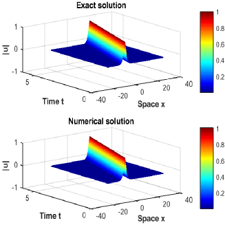
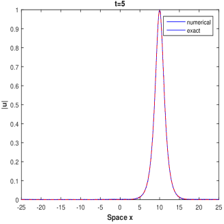
Figure 1: Comparison of the analytic solution and the numerical solution with $x_{0}=10,\theta=1,h=0.5,\tau=0.001$ and $\mathbf{k}=2$.

As is stated in Theorem 3.1, the LDG method (3)-(4) could preserve the discrete charge conservation law exactly. We consider this phenomenon numerically in Fig. 2, where the figure shows the global error. We can see that the global residual of the discrete charge conservation law reaches the magnitude of $10^{-15}$. Thus, we observe a good agreement with the theoretical result.

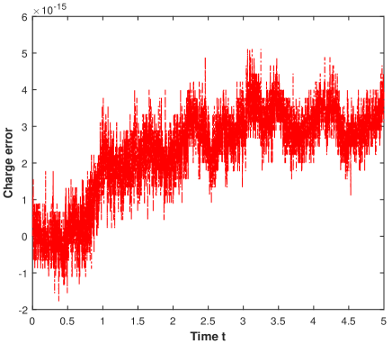
Figure 2: The global error of the discrete charge conservation law of single soliton with $x_{0}=10,\theta=1,h=0.5,\tau=0.001$ and $\mathbf{k}=2$.

4.2 The Interaction of Double Soliton

In this experiment, we show the double soliton collision of Eq. (21) with the initial condition

$$u_{0}(x)={\rm sech}(x-x_{1})e^{2\mathbf{i}c_{1}(x-x_{1})}+{\rm sech}(x-x_{2})e^{2\mathbf{i}c_{2}(x-x_{2})}.$$

The global error of the discrete charge conservation law is shown in Fig. 3. Again, we observe the phenomena which agrees with the theoretical result.

Figure 3: The global error of the discrete charge conservation law of double soliton with $c_{1}=1$, $c_{2}=-1$, $x_{1}=-10$, $x_{2}=10,\theta=1,h=0.5,\tau=0.001$ and $\mathbf{k}=2$.

The evolution on the interval $[0;5]$ is shown in Fig. 4 and the profiles at different instants in Fig. 5. We observe that the interaction is elastic and the two waves emerges without any changes in their shapes and they conserve the energy almost exactly.

Figure 4: Collision of two solitons whose parameters are $c_{1}=1,c_{2}=-1,x_{1}=-10,x_{2}=10,\theta=1,h=0.2,\tau=0.001$ and $\mathbf{k}=2$.

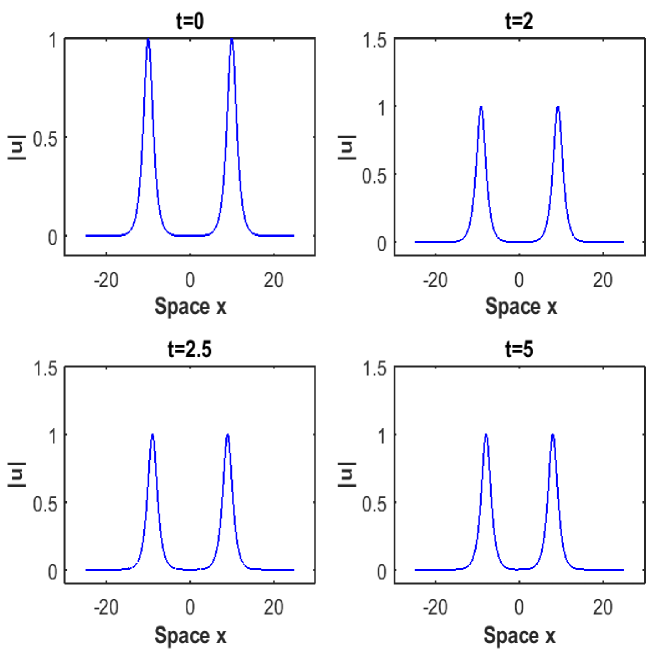
Figure 5: Profiles at time $t=0,~{}2,~{}2.5$ and $5$ of Fig. 4.

4.3 The Birth of Mobile Soliton

In this experiment, we show the birth of soliton using a square well initial condition

$$u_{0}(x)=Ae^{-x^{2}+2\mathbf{i}x}.$$

In Figs. 6-7, the mobile soliton is observed.

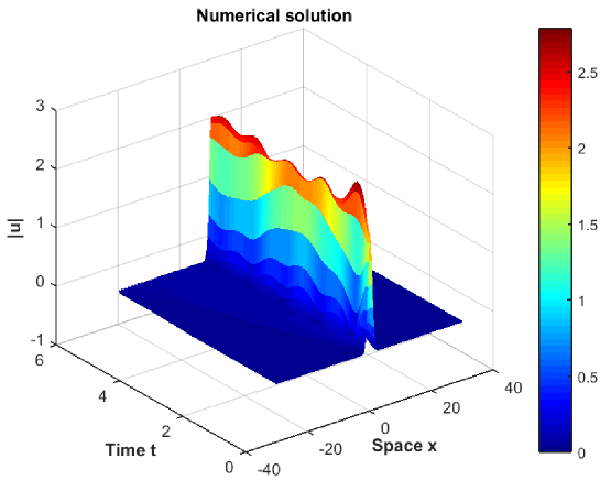
Figure 6: The birth of mobile soliton. $A=2,\theta=1,h=0.2,\tau=0.001$ and $\mathbf{k}=2$. Periodic boundary condition in $[-30,30]$.

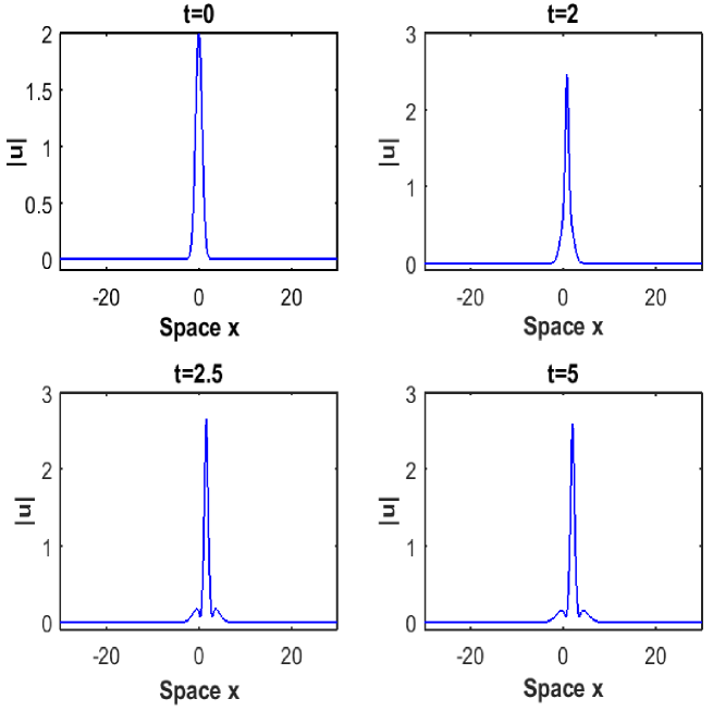
Figure 7: Profiles at time $t=0,~{}2,~{}2.5$ and $5$ of Fig. 6.

4.4 Optimal Convergence Estimates

We show an accuracy test for Eq. (21) with the soliton solution

$$u(t,x)={\rm sech}(x+x_{0}-4t)e^{2\mathbf{i}(x+x_{0}-3t/2)}.$$

We take the temporal step-size $\tau=0.00001$, and the time interval $[0,1]$, the numerical spatial domain $\mathcal{O}=[-30,30]$ with the periodic boundary condition.

Table 1 lists the $\mathbb{L}^{2}$-errors and their numerical orders with different values of $\theta$ at $T=1$. From the table we conclude that, for all values of $\theta\in[0,1]$, one can always observe $(\mathbf{k}+1)$-th order of accuracy in $\mathbb{L}^{2}$-norm.

	$N$	$\mathbb{L}^{2}$-error	Order
	60	3.54E-1	-
	120	7.20E-2	2.70
$\theta=0.4$	240	1.36E-2	3.02
	480	2.43E-3	3.04
	60	2.31E-1	-
	120	2.33E-2	3.73
$\theta=0.5$	240	3.89E-3	3.45
	480	6.91E-4	2.93
	60	2.30E-1	-
	120	2.89E-2	3.24
$\theta=1$	240	4.54E-3	3.68
	480	7.51E-4	2.94

	$N$	$\mathbb{L}^{2}$-error	Order
	60	8.72E-2	-
	120	6.58E-3	3.94
$\theta=0.4$	240	5.64E-4	3.90
	480	4.82E-5	3.91
	60	1.94E-2	-
	120	2.18E-3	3.50
$\theta=0.5$	240	2.02E-4	3.87
	480	1.84E-5	3.80
	60	2.91E-2	-
	120	2.99E-3	3.84
$\theta=1$	240	2.64E-4	3.80
	480	2.67E-5	3.97

Table 1: Accuracy test for Eq. (NLS) using $\mathbb{P}^{2}$ polynomials (left) and $\mathbb{P}^{3}$ polynomials (right) with different $\theta$.

5 Conclusion

In this paper, we develop an LDG method to solve the one-dimensional nonlinear Schrödinger equation. The charge conservation law is shown to be preserved for LDG method proposed in this paper. The CLDG method, when applied to NLS equation, is shown to have the optimal $(\mathbf{k}+1)$-th order of accuracy for polynomial elements of degree $\mathbf{k}$. The numerical tests demonstrate both accuracy and capacity of the method.

References

- [1] Y. Cheng, X. Meng, and Q. Zhang. Application of generalized Gauss-Radau projections for the local discontinuous Galerkin method for linear convection-diffusion equations. To appear at Math. Comp.
- [2] P. G. Ciarlet. The finite element method for elliptic problems. North-Holland Publishing Co., Amsterdam-New York-Oxford, 1978. Studies in Mathematics and its Applications, Vol. 4.
- [3] B. Cockburn and C.-W. Shu. The local discontinuous Galerkin method for time-dependent convection-diffusion systems. SIAM J. Numer. Anal., 35(6):2440–2463 (electronic), 1998.
- [4] B. Cockburn and C.-W. Shu. Runge-Kutta discontinuous Galerkin methods for convection-dominated problems. J. Sci. Comput., 16(3):173–261, 2001.
- [5] J. Ginibre and G. Velo. On the global Cauchy problem for some nonlinear Schrödinger equations. Ann. Inst. H. Poincaré Anal. Non Linéaire, 1(4):309–323, 1984.
- [6] T. Lu, W. Cai, and P. Zhang. Conservative local discontinuous Galerkin methods for time dependent Schrödinger equation. Int. J. Numer. Anal. Model., 2(1):75–84, 2005.
- [7] X. Meng, C.-W. Shu, and B. Wu. Optimal error estimates for discontinuous Galerkin methods based on upwind-biased fluxes for linear hyperbolic equations. Math. Comp., 85(299):1225–1261, 2016.
- [8] C.-W. Shu. Discontinuous Galerkin methods: general approach and stability. In Numerical solutions of partial differential equations, Adv. Courses Math. CRM Barcelona, pages 149–201. Birkhäuser, Basel, 2009.
- [9] Y. Xing, C.-S. Chou, and C.-W. Shu. Energy conserving local discontinuous Galerkin methods for wave propagation problems. Inverse Probl. Imaging, 7(3):967–986, 2013.
- [10] Y. Xu and C.-W. Shu. Local discontinuous Galerkin methods for two classes of two-dimensional nonlinear wave equations. Phys. D, 208(1-2):21–58, 2005.
- [11] Y. Xu and C.-W. Shu. Local discontinuous Galerkin methods for high-order time-dependent partial differential equations. Commun. Comput. Phys., 7(1):1–46, 2010.
- [12] Y. Xu and C.-W. Shu. Optimal error estimates of the semidiscrete local discontinuous Galerkin methods for high order wave equations. SIAM J. Numer. Anal., 50(1):79–104, 2012.
- [13] J. Yan and C.-W. Shu. A local discontinuous Galerkin method for KdV type equations. SIAM J. Numer. Anal., 40(2):769–791 (electronic), 2002.
- [14] R. Zhang, X. Yu, and T. Feng. Solving coupled nonlinear Schrödinger equations via a direct discontinuous Galerkin method. Chin. Phys. B, 21(3):30202–1–30202–5, 2012.
- [15] R. Zhang, X. Yu, and G. Zhao. A direct discontinuous Galerkin method for nonlinear Schrödinger equation (in chinese). Chin. J. Comput. Phys., 29(2):175–182, 2012.