Lens model and time delay predictions for the sextuply lensed quasar SDSS J2222$+$2745

Abstract

SDSS J2222$+$2745 is a galaxy cluster at $z=0.49$, strongly lensing a quasar at $z=2.805$ into six widely separated images. In recent HST imaging of the field, we identify additional multiply lensed galaxies, and confirm the sixth quasar image that was identified by Dahle et al. (2013). We used the Gemini North telescope to measure a spectroscopic redshift of $z=4.56$ of one of the secondary lensed galaxies. These data are used to refine the lens model of SDSS J2222$+$2745, compute the time delay and magnifications of the lensed quasar images, and reconstruct the source image of the quasar host and a second lensed galaxy at $z=$2.3. This second galaxy also appears in absorption in our Gemini spectra of the lensed quasar, at a projected distance of 34 kpc. Our model is in agreement with the recent time delay measurements of Dahle et al. (2015), who found $\tau_{\rm AB}$=$47.7\pm{6.0}$ days and $\tau_{\rm AC}$=$-722\pm{24}$ days. We use the observed time delays to further constrain the model, and find that the model-predicted time delays of the three faint images of the quasar are $\tau_{\rm AD}$=$502\pm{68}$ days, $\tau_{\rm AE}$=$611\pm{75}$ days, and $\tau_{\rm AF}$=$415\pm{72}$ days. We have initiated a follow-up campaign to measure these time delays with Gemini North. Finally, we present initial results from an X-ray monitoring program with Swift, indicating the presence of hard X-ray emission from the lensed quasar, as well as extended X-ray emission from the cluster itself, which is consistent with the lensing mass measurement and the cluster velocity dispersion.

1. Introduction

The rare chance alignment of a quasar behind a strong-lensing cluster provides unique opportunities for studies of different astrophysical objects. Through careful lens modeling, these systems can probe the mass distribution of the foreground lens; the high magnification enhances our ability to study the background quasar, and galaxies between us and the quasar can be seen in absorption along multiple lines of sight in the light of the background quasar. Lensing configurations that involve a quasar lensed by a single massive galaxy are more common; however, the lensing magnification of a single galaxy is typically significantly lower than in the galaxy cluster case. Unique to the cluster-lensed quasar configurations, the multiple images of the lensed quasar have large separations ($14\farcs 6-22\farcs 5$; Inada et al. 2003, 2006; Dahle et al. 2013) and high magnifications; the lensed active nucleus is point-like, providing accurate positional constraints, and is variable –- enabling measurements of the time delay between images of the same source. The high tangential magnification stretches the host galaxy of the quasar into a giant arc, thus resolving it from the light of the active nucleus, which usually dominates in a high-redshift quasar.

To date, only three cases of high-redshift quasars strongly-lensed by a galaxy cluster are published: SDSS J1004+4112 (Inada et al. 2003), SDSS J1029+2623 (Inada et al. 2006), and SDSS J2222$+$2745 (Dahle et al. 2013).

SDSS J2222$+$2745 was discovered as part of the Sloan Giant Arcs Survey (SGAS; Gladders et al. in prep, Bayliss et al. 2011a,b; Hennawi et al. 2008; Sharon et al. 2014). SGAS is a systematic survey of highly magnified lensed galaxies, also refered to as “giant arcs,” in the imaging data of the Sloan Digital Sky Survey (SDSS, York et al. 2000). The lensing identification process starts with optical selection of galaxy clusters from the SDSS photometry catalogs, using the cluster red sequence algorithm of Gladders & Yee (2000). Sections of the imaging data around each cluster were then retrieved and processed to generate color images, with scaling parameters selected to optimize the visibility of possible lensing features. The images were visually inspected and ranked for lensing evidence by several observers in a process that enables a calculation of the selection statistics (the process will be described in full in Gladders et al., in preparation). All candidates were followed up for confirmation, and the survey purity and completeness were quantified. Bayliss et al. (2011a,b) give the results of the initial spectroscopic followup campaign, and measure the redshift distribution of the lensed galaxies.

SDSS J2222$+$2745 was detected in the SGAS search in SDSS Data Release 8 (Aihara et al. 2011) owing to a prominent giant arc that appears $8\farcs 5$ south of the brightest cluster galaxy. A further investigation of the field revealed the multiply-imaged lensed quasar. The field was followed up by Dahle et al. (2013) using the Mosaic Camera (MOSCA) and the Andalucia Faint Object Spectrograph and Camera (ALFOSC) at the 2.56 m Nordic Optical Telescope (NOT).

We have recently obtained HST imaging data of this target (Figure 1; Section 2). As can be seen in Figure 1, a background quasar is lensed by SDSS J2222$+$2745, forming six images around the core of a galaxy cluster at $z=$0.49. Three bright images appear north of the cluster core (labeled A, B, C; our labeling scheme follows Dahle et al. 2015), and three faint images (D, E, F) can be seen near the central cluster galaxies (G2, G3, G1, respectively). The cluster also lenses other background galaxies, the most prominent of which is seen as a blue arc south of the cluster core (labeled A1 in Figure 1). Dahle et al. (2013) reported on the discovery of SDSS J2222$+$2745, confirmed the lensing interpretation, presented spectroscopic identification of the lensed quasar, spectroscopic confirmation of the six lensed images of the quasar, and measured its redshift to be $z=2.82$. In addition, we measured the spectroscopic redshifts of several cluster member galaxies, and of the lensed galaxy A1 at $z=$2.3. Stark et al. (2013) also measure the spectra of the quasar, $z=2.807$ and of galaxy A1. Interestingly, the spectrum of the quasar shows strong Ly$\alpha$ absorption at the redshift of the foreground lensed galaxy, as well as Si II $\lambda$1526 and CIV $\lambda$1549 (Stark et al. 2013), indicating the presence of neutral hydrogen and metals associated with gas surrounding the galaxy. Stark et al. (2013) estimated that the projected distance between the quasar image A and the interloper galaxy A1 is $\sim 50$ kpc. We refine this estimate in Section 4.5.

Following the discovery of SDSS J2222$+$2745, we have initiated an imaging monitoring program with the NOT to measure the time delays between the images of the quasar. The results from the first three years of ongoing photometric monitoring with the NOT and the first season of Gemini monitoring are presented in Dahle et al. (2015). The light curves of the brighter three images of SDSS J2222$+$2745 are measured from an analysis of 42 distinct epochs, resulting in time delays of $\tau_{\rm AB}$=$47.7\pm{6.0}$ days, and $\tau_{\rm AC}$=$-722\pm{24}$ days. A robust measurement of the time delays of images D, E, and F requires deeper observations; a monitoring campaign with Gemini was initiated in 2015 (GN-2016A-Q-28; PI: Gladders) for this purpose.

This paper is structured as follows. In Section 2 we describe the HST imaging data of SDSS J2222$+$2745, Gemini spectroscopy, and Swift X-ray observations. We present a new strong lensing analysis based on the new data in Section 3. In Section 4, we present and discuss the predicted time delays, cluster mass, lensing magnification, source reconstruction, and absorbing systems. We conclude with future work in Section 5. Throughout this paper, we assume a flat cosmology with $\Omega_{\Lambda}=0.7$, $\Omega_{m}=0.3$, and $H_{0}=70$ km s^-1 Mpc^-1. In this cosmology, $1\arcsec$ corresponds to 6.0384 kpc at the cluster redshift, $z=$0.49. Magnitudes are reported in the AB system.

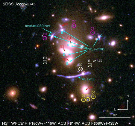
Figure 1.— Color composite image of SDSS J2222$+$2745 from our HST program GO-13337 (PI: Sharon) in WFC3/IR F160W+F110W (red), ACS F814W (green), ACS F606W+F435W (blue). These data confirm the sixth quasar image (F) that was identified by Dahle et al. (2013) as tentative. The six images of the lensed quasar at $z=2.805$ and the previously identified giant arc A1 at $z=2.3$ are labeled in cyan; newly discovered secure multiply-imaged galaxies are labeled in white (B1, B2, B3 at $z=4.56$, see § 2.2), yellow (D1, D2, D3) and magenta (C1, C2, C3). Other possible arc candidates are not labeled. Note that the point source that is seen embedded in the A1 arc is a foreground white dwarf star (Dahle et al. 2013).

2. Data

2.1. HST Imaging

SDSS J2222$+$2745 was observed by HST Cycle 21 program GO-13337 (PI: Sharon) with WFC3 F160W for 1311 s and F110W for 1211 s on 2014 Aug 10, and with ACS F435W, F606W, and F814W for 4944 s each on 2014 Oct 10-11 . The filters were carefully selected to provide the best sensitivity to the different sources in the field. The bluest filter, F435W, is sensitive to emission from the quasar and its host and gives high contrast between the quasar and the cluster galaxies, as can be seen in Figure 2. At $z$=0.49 most of the light from typical elliptical galaxies is redshifted to wavelengths longer than the ACS/F435W response curve, and we expect to see little emission in this band from the cluster galaxies. ACS/F606W and ACS/F814W give good sampling of the spectral energy distribution of typical early-type cluster galaxies; and the reddest filters help detect lensed high-$z$ dropout galaxies and provide a long wavelength baseline for galaxy colors and SED fitting.

Each of the ACS images was taken over two orbits, with three gap-crossing sub-pixel dither positions in each orbit (a total of six sub-exposures) for better sampling of the point spread function, removal of cosmic rays, hot or bad pixels, and to cover the chip gaps. A half field-of-view offset was implemented between the two orbits of observation in each filter. Since the strong lensing regime is small enough to fit within one ACS chip, this design ensures that the center of the field is imaged to the full depth of two orbits per filter, which is needed to obtain the required signal to noise, while at the outskirts we allowed shallower exposure. The increased field of view enables studies that require high resolution at somewhat larger cluster-centric radii, including weak lensing measurements, selection of cluster member galaxies for strong lensing analysis, and galaxy cluster science.

The WFC3-IR observations were executed within a single orbit, four images per filter with small box dithers for PSF reconstruction and to cover artifacts such as the “IR Blobs” and “Death Star” (WFC3 Data Handbook; Rajan et al. 2011). We used sampling interval parameter SPARS25.

The subexposures of each filter were reduced and combined following the reduction pipeline of our Cycle-20 program GO-13003 (e.g., Sharon et al. 2014). The WFC3-IR images were treated using a custom algorithm to remove the “IR Blobs”, and we corrected the ACS images for CTE losses prior to drizzling. Individual corrected images were combined using the AstroDrizzle package (Gonzaga et al. 2012) with a pixel scale of $0\farcs 03$ pixel^-1, and drop size of 0.5 for the IR filters and 0.8 for the ACS filters. This approach provides good recovery of the PSF in all bands and maximizes the sensitivity to detail. All images were aligned onto the same pixel frame. In the final reduced data, the $5\sigma$ limiting magnitudes in the five filters are 27.4, 27.8, 27.3, 26.8, and 26.5 mag within a circular aperture of diameter $0\farcs 7$, for F435W, F606W, F814W, F110W, and F160W, respectively.

A photometric catalog of all the objects in the overlapping ACS and WFC3 field of view was generated following procedures outlined in Skelton et al. (2014), and spectral energy distribution (SED) fits and photometric redshifts derived using EAZY (Brammer et al. 2008). We note that the fidelity of the photometric redshift is limited by the small number of filters, nevertheless, the photometric redshifts are found to be consistent with the available spectroscopic redshifts.

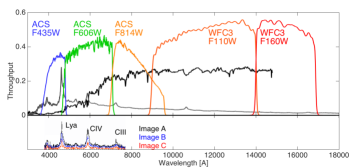
Figure 2.— The response function of the five filters that were used in the HST observation (GO-13003; PI: Sharon) overplotted on a template spectrum of an elliptical galaxy, redshifted to the cluster redshift, $z=0.49$ (black), and a template quasar spectrum redshifted to the quasar redshift, $z=2.805$ (gray). The filters sample the spectral energy distribution of cluster galaxies as well as the quasar and its host, and provide good contrast between these sources. The broad wavelength coverage supports SED fitting and identification of secondary arcs. Bottom: Spectra of images A, B, and C of the quasar from Dahle et al. (2013).

2.2. Gemini Spectroscopy

The main scientific goal of the HST observations was to facilitate a detailed lens model of SDSS J2222$+$2745. Strong lens modeling relies on constraints from observational evidence of strong lensing, in the form of multiple images of lensed background sources. The positions and redshifts are used as local solutions of the lensing equations to constrain the projected mass density distribution at the core of the cluster. The accuracy of a lens model strongly depends on the availability of lensing constraints. The mass distribution and lensing magnification are sensitive not only to the accurate identificaitons and positions of multiple images, but also to the redshifts of these lensed galaxies. This is especially important when there are few lensed sources identified (Johnson & Sharon 2016). Lens models that are computed with no spectroscopic redshifts as constraints are shown to produce erroneous results (e.g., Smith et al. 2009, Johnson & Sharon 2016); it is therefore critical to include constraints from at least a few spectroscopically-confirmed source redshifts.

We were awarded 4.5 hours of Band One queue observations with Gemini Multi-Object Spectrograph (GMOS; Hook et al., 2004) on the Gemini North telescope (GN-2015B-Q-27; PI: Sharon) to secure spectroscopic redshifts of the secondary arcs that were identified in the new HST data.

Observations of this program were executed on UT 2015 Sep 10 and 2015 Nov 6 & 7. Conditions at the times of observation were photometric, with seeing between $0\farcs 5-0\farcs 85$. The field was imaged by our NOT/ALFOSC monitoring program during the same dark runs, indicating little variability between these epochs; we report the $g$-band photometry for reference: On 2015 Sep 13.16, g(A)=21.67; g(B)=22.07; g(C)=21.76. On 2015 Nov 07.90, g(A)=21.71 mag; g(B)=21.98 mag; g(C)=21.52 mag.

For the Gemini/GMOS observations, GMOS was configured in macro nod-and-shuffle (N&S) mode with the R400_G5305 grating in first order and the G515_G0306 long pass filter. The detector was binned by a factor of 2 in the spectral direction and unbinned spatially. Following extensive previous experience using GMOS in this mode (e.g., Bayliss et al., 2011b, 2014) we chose a N&S cycle length of 120 s as a balance between achieving good sampling of time variation in the sky and limiting charge trap effects by minimizing the number of shuffles in a given integration.

We designed two multi-object slit masks that preferentially placed slits on faint candidate strongly lensed background sources around the core of SDSS J2222$+$2745 (see Figure 3 for mask design and Figure 1 for source IDs). Mask 1, at position angle of 65 degrees, targeted lensing candidate images B1, B2, B3, C2, D1, D3, a faint edge of A1, image C of the quasar and image A of the host galaxy of the quasar. Mask 2 at position angle of 47 degrees targeted arc A1, B1, C3, D2 and quasar images A, B, C, and D. Both masks targeted cluster member galaxies and other galaxies in the field.

Slits were placed so as to target high-priority sources at both the original pointing position and the offset nod position; this slit strategy is the same as described in Bayliss et al. (2011b), and we refer to that paper for a detailed description. Most slits on each mask were 1″ wide, with lengths varying from slit to slit. Two slits on each mask had widths of $0\farcs 5$; these were placed on the three brightest red galaxies in the core of the cluster to produce higher resolution spectra, which may potentially inform stellar velocity dispersion measurements for those galaxies. Each spectroscopic mask was exposed twice for 2400 s, with a wavelength dither between the exposures to cover the chip gaps in the GMOS detector array.

We reduced the resulting GMOS spectra using a suite of custom tools that was developed using the XIDL package; this pipeline is similar to that used in Bayliss et al. (2014). For N&S spectra sky subtraction simply requires differencing the two shuffled sections of the detector. We first performed this differencing of the raw spectra, and then wavelength calibrated, extracted, stacked, and flux normalized spectra from each slit on each of the two masks. Flux calibration was performed using an archival standard star. The archival calibration provides a reliable relative flux correction, but does not yield an absolute flux calibration. The spectral resolution of the final data is R $\simeq 700-1100$ ($270-430$ km s^-1) for spectra taken through 1″ wide slits, and R $\simeq 1400-2200$ ($135-215$ km s^-1) for spectra taken through $0\farcs 5$ wide slits.

We summarize the results of the Gemini spectroscopy observations in Table 1. Details of the spectroscopic analysis of the high priority sources are given below.

Quasar images: We refine the redshift measurement of the quasar, and obtain $z=2.8050\pm 0.0006$ from the spectra of images A, B, C of the quasar (Figure 4, top panel). We observe emission lines from HeII 1640, OIII] 1666, [OII] 2470, and CII] 2327, and CIV 1549. We also detect absorption lines from MgII and other elements at $z=2.296$, from the intervening galaxy A1 (see Section 4.5). The spectrum of image D is dominated by light from the foreground cluster galaxy, however, CIV and CIII emission lines from the quasar can be detected. A slit targeting the host galaxy of image A of the quasar (see Figure LABEL:fig.mask for slit placement) resulted in low S/N spectrum that is dominated by light from the nucleus.

Lensed galaxy A1: From two slitlets in Mask 2, we confirm the known arc redshift of $z=$2.3 from ISM absorption lines Fe II 2344, 2382; Fe II 2586,2600; and MgII 2798, 2803. We identify weak nebular emission of Si III] 1892, and C III] 1909. The combined spectrum is shown in Figure 4. The slitlet that targeted the faint region of the arc did not result in sufficient S/N.

Lensed galaxy B: Figure 4 shows stacked spectra of arc B1 from four slitlets, two in Mask 1 and two in Mask 2. We identify emission lines from Ly$\alpha$, SiII 1260, OI+SiII 1303, HeII 1640, and CIV 1449 at $z=4.56$. The images of B drop out completely from the ACS/F435W filter, which supports this redshift interpretation. Furthermore, the photometric redshift analysis obtained for this source from the five HST bands shows a single high significance peak around $z_{\rm phot}=4.4$. The slits placed on B2 and B3 resulted in too low S/N for an independent measurement of the redshift. Nonetheless we detect a faint emission line in these spectra that is consistent with Ly$\alpha$ at the same redshift as image B1.

Lensed galaxy C: We targeted C2 and C3, with a total on-target exposure time of 2400 s on each image; however since these sources are faint, the resulting spectra have low S/N. A possible absorption line is detected at 6210 Å. Interpreting this absorption feature as the CIV 1548,1550 lines, which are often among the most prominent rest-frame UV features in star-forming galaxies, places this source at z=3.01. We note that this putative spectroscopic redshift is also consistent with the photometric redshift analysis and favored by the lensing analysis. Nevertheless, given its low certainty we do not consider this a secure spectroscopic redshift for the purpose of lensing analysis.

Lensed galaxy D: We placed slitlets on D1, D2, and D3. As can be seen in Figure 3, the slits are expected to contain light from adjacent sources (in particular, blue emission from a nearby galaxy). The spectroscopic analysis results in a low confidence redshift of $z=0.837$ for D1 and D2, based on Ca H&K lines, and no signal in D3. The photometric redshift probability distribution function is bimodal, with a high significance peak around $z=4.4$ and low-significance peak around $z=0.74$ for images D1 and D3. Image D2 shows only one peak at $z=0.74$. Since this is the image that is most contaminated by blue light from the nearby galaxy, we argue that this interpretation is consistent with two separate redshifts for two different background sources. A blue arc at low-z, consistent with the possible $z=0.837$ that is suggested by the spectroscopy, and a high redshift source at $z\sim 4.4$ which is likely the three-imaged lensed source D. Due to the ambiguous redshift interpretation, we leave this redshift as a free parameter as well, with upper redshift prior $z<5$ set by the photometric redshift analysis.

Cluster galaxies: We measure spectroscopic redshifts of 11 cluster galaxies, including the central galaxies G1, G2, G3 and G4. These measurements confirm the published spectroscopic redshifts of G1, G2, G3 from the NOT (Dahle et al. 2013). In the spectrum of galaxy G3 we detect weak C IV emission at $z$=2.805 from the embedded quasar image E. In Table 1 we also list the redshifts of three galaxies with SDSS-DR9 spectroscopy that are within projected radius of 1500 h^-1 kpc from the BCG. From these 14 members we measure a cluster redshift of $z=0.4897\pm 0.0032$, and a velocity dispersion of $\sigma_{v}=657\pm 166$ km s^-1, using the Gapper estimator (Beers et al. 1990). The uncertainties on the velocity dispersion are calculated as $\pm 0.91\sigma_{v}/\sqrt{n-1}$, where $n$ is the number of galaxies, following Ruel et al. (2014). Using the mass scaling relation in Evrard et al. (2008), the velocity dispersion translates to a dynamical mass of $M_{200,{\rm dynamical}}=3.9^{+3.6}_{-2.2}\times 10^{14}$ M_⊙.

Other galaxies: Table 1 also lists the coordinates and the spectroscopic redshifts of other background (i.e., behind the cluster) and foreground galaxies in the field that were measured from these data.

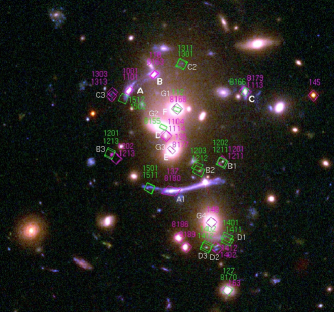
Figure 3.— The sources that were targeted for Gemini-North Gmos multislit spectroscopy are labeled in green (Mask 1) and red (Mask 2). Faint sources were targeted by both masks or in both nod positions, in order to maximize their signal to noise.

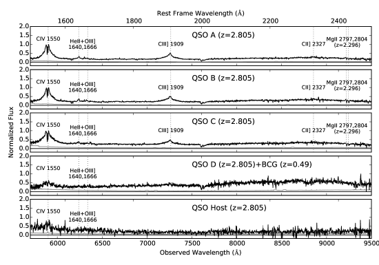
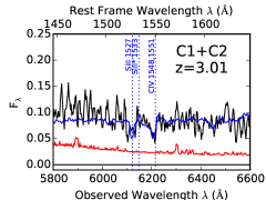
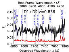
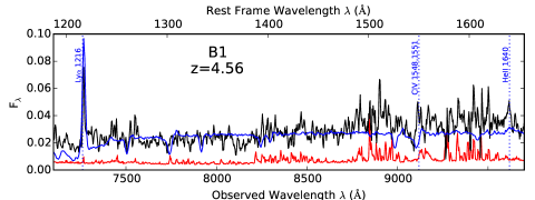
Figure 4.— Gemini/GMOS spectra of the quasar and arcs A, B, C, D in SDSS J2222$+$2745. The noise level is plotted in magenta. Emission and absorption lines are noted. In blue, we overplot the composite stacked spectra of Lyman Break Galaxies from Shapley et al. (2003).

Table 1Lensing Constraints and Spectroscopy Results

ID	R.A.	Decl.	Redshift	mask obj. ID	Comments
	[J2000]	[J2000]
QSO-A	335.537707	27.760543	$2.8050\pm 0.0006$	2-1001, 2-1101	HeII 1640+OIII]1666+[OII]2470 emission
QSO-B	335.536690	27.761119	$2.8048\pm 0.0005$	2-118, 2-8163	HeII 1640+OIII]1666 emission
QSO-C	335.532960	27.760505	$2.8050\pm 0.0006$	1-8166, 2-1113,	HeII 1640+CII]2327+[OII]2470 emission
				2-8179
QSO-D	335.536205	27.758901	$2.8012\pm 0.0005$	2-1104, 2-1114	Dominated by light from G2; redshift from CIV+CIII]
QSO-E	335.536007	27.758248	$\cdots$	$\cdots$	No new data; spec confirmed by Dahle et al. (2013)
QSO-F	335.535874	27.759723	$\cdots$	$\cdots$	No new data; spec confirmed by Dahle et al. (2013)
QSO-host-A	335.537968	27.760220	$2.8$	1-1502, 1-1512	Low S/N; Dominated by quasar spectrum
A1	335.536022	27.756889	$2.2963\pm 0.0004$	2-137, 2-8180	NIII] 1750, SiIII] 1892, CIII] 1909 Nebular emission
A1	335.536909	27.756990	$\cdots$	1-1501, 1-1511	Faint end; No signal
B1	335.53388	27.757979	$4.562\pm 0.002$	1-1202, 1-1211	Shapley composite comparison; Ly$\alpha$ at z=4.5651,
				2-1201, 2-1211	HeII 1640 at z=4.5564
B2	335.534820	27.757630	$\cdots$	1-1212, 1-1213	low S/N or contaminated
B3	335.538410	27.758236	$\cdots$	2-1201, 2-1213	low S/N or contaminated
C1	335.533620	27.760879	$\cdots$	$\cdots$	$\cdots$
C2	335.538420	27.760385	$\cdots$	1-1311	low S/N (see text)
C3	335.538425	27.760429	$\cdots$	1-1303, 1-1313	low S/N (see text)
D1	335.533530	27.755175	($0.837\pm 0.002$)	1-1411, 1-1401	Uncertain redshift; probably contaminated by FG object.
D2	335.534090	27.754942	($0.836\pm 0.001$)	2-1402, 2-1412	Uncertain redshift; probably contaminated by FG object.
D3	335.534540	27.754882	$\cdots$	1-1412, 1-1402	Sky position contaminated
cluster gal G1	335.535793	27.759830	$0.4901\pm 0.0002$	1-112, 2-8168	cluster galaxy
cluster gal G2	335.536366	27.759190	$0.4925\pm 0.0002$	1-8155	cluster galaxy, $0\farcs 5$ slit
cluster gal G3	335.536022	27.758369	$0.4919\pm 0.0004$	2-135, 2-8177	cluster galaxy, z=2.8055 CIV emission from QSO-E
cluster gal G4	335.534391	27.755760	$0.4922\pm 0.0002$	2-148	cluster galaxy
cluster gal	335.525723	27.738350	$0.4906\pm 0.0008$	2-232	cluster galaxy
cluster gal	335.527496	27.751221	$0.4902\pm 0.0004$	2-186	cluster galaxy
cluster gal	335.533733	27.753309	$0.4861\pm 0.0003$	1-8170, 2-163	cluster galaxy
cluster gal	335.536966	27.744699	$0.4945\pm 0.0006$	2-176	cluster galaxy
cluster gal	335.553675	27.773190	$0.4913\pm 0.0002$	2-8104	cluster galaxy
cluster gal	335.535707	27.755211	$0.4893\pm 0.0007$	2-8186	cluster galaxy
cluster gal	335.535421	27.754869	$0.4883\pm 0.0006$	2-8189	cluster galaxy
BG	335.517597	27.782749	$0.732\pm 0.001$	2-8155	background
BG	335.546093	27.751680	$0.6031\pm 0.0002$	1-8145, 2-119	background, strong nebular emission, likely NL AGN
BG	335.516653	27.766451	$0.8813\pm 0.0001$	2-169	background, star foming; strong nebular emission
FG	335.505838	27.762159	$0.3490\pm 0.0001$	1-194	foreground, strong H$\alpha$
FG	335.520544	27.755730	$0.4487\pm 0.0002$	2-196	foreground
cluster gal	335.546740	27.758008	0.4833 $\pm$ 0.0001	$\cdots$	SDSS-DR9
cluster gal	335.535580	27.772658	0.4883 $\pm$ 0.0001	$\cdots$	SDSS-DR9
cluster gal	335.503210	27.789785	0.4843 $\pm$ 0.0001	$\cdots$	SDSS-DR9

Note. — Spectroscopic redshifts, from Gemini/GMOS observations, of images of the quasar, lensed galaxies, cluster member, foreground and background galaxies. The coordinates of the six images of the quasar, as well as galaxies B1-3, C1-3, and D1-3 correspond to the exact coordinate of their peak brightness, that was used as lensing constraint. Otherwise, the coordinates on which the slits were placed are given. Due to the uncertain spectroscopy result for arc C and D, we left their redshifts as free parameters with a priors set by photometric redshift analysis, $2.0\leq z_{C}\leq 4.0$ and $3.8\leq z_{D}\leq 5.0$. All other redshifts were fixed to their spectroscopic measurements. Stars and slits with insufficient data quality are not shown. See also Figure 3.

2.3. SWIFT X-ray Observations

SDSS J2222$+$2745 was observed at X-ray wavelengths by the Swift X-ray telescope (XRT) as part of a monitoring program using University of Michigan time (PI: Sharon). Observations were taken approximately every six weeks over seven epochs between 2015 September 16 and 2016 June 29, with a combined exposure time of 90.5 ks. The typical exposure time was 15 ks per epoch with the exception of epoch 1 that was observed for $\sim$10 ks (see Table 2). The hard X-ray radiation ($<3$ keV) varies during this time by up to a factor of three between epochs with the lowest and the highest counts per second, confirming the variable nature of the quasar at these wavelengths. However, the Swift XRT resolution (see below) is not sufficient to robustly resolve the three brightest images of the lensed quasar. A decomposition analysis of the variable emission is beyond the scope of this paper, and will be presented in future work. Here, we present the co-added data from the first seven epochs, and analyze the X-ray emission from the cluster hot gas.

The data were reprocessed using the HEASOFT v. 6.17 and the most up-to-date version of CALDB, accessible via remote server. New Level 2 event files were created using the tool xrtpipeline. We used the XRT Data Product Generator to combine images from different epochs, and for astrometric measurements. We verified the absolute astrometric solution by matching the coordinates of a bright X-ray star at [RA, Dec]=[335.39729, 27.707253], with its optical counterpart from the SDSS.

The Swift XRT has a PSF of $18^{\prime\prime}$ at 1.5 keV; at this resolution, the X-ray radiation from the images of the lensed quasar is blended with the diffuse emission from the hot cluster X-ray gas. Nevertheless, their contribution is wavelength dependent, with the soft X-ray radiation ($\lesssim 3$ keV) dominated by the cluster emission, and the hard X-ray photons attributable to the quasar. In order to separate the cluster emission from the quasar emission, we co-add the emission in the $0.3-3.0$ keV range from all seven epochs. The resulting X-ray contours are over-plotted on the optical image in Figure 5. We find that the soft X-ray emission is centered on [RA, Dec]=[335.53613, 27.760667], with a 90% confidence error radius of $3\farcs 0$ (see Evans et al. 2014 for more information on the way the astrometric position is determined). This position is in excellent agreement with the center of the main cluster halo component as derived from the lensing analysis (Section 3). The two centroids are $1\farcs 11$ in projection, a distance which is within the $3\farcs$ XRT astrometric uncertainty. Nevertheless, since the XRT Data Product Generator is not optimized for measurements of extended sources the uncertainty may be underestimated.

For an estimate of the cluster mass, we measure the background-subtracted X-ray flux, from the co-added data of the seven epochs, in the energy range 0.1-2.4 keV, within an aperture of radius 1 Mpc centered on the cluster; we assume that this radius corresponds roughly to R₅₀₀ (e.g., Mantz et al. 2010), and that in this energy range the X-ray radiation is dominated by the cluster with negligible contamination from the background quasar. To account for errors due to the unknown gas temperature we consider a range of gas temperatures between kT=[$3.06-9.67$] keV, and find luminosities in the range $L{\rm x}=[1.0-1.4]\times 10^{44}$ ergs s^-1. The luminosity is within the range expected for clusters with similar velocity dispersion (Xue & Wu 2000). We use the Mantz et al. (2010) $M-L_{\rm X}$ relation to estimate the cluster mass, $M_{500,{\rm x}}=[0.94-1.2]\times 10^{14}$ M_⊙. The X-ray-inferred mass estimate is in line with the lensing mass measurement and with the dynamical mass. A more robust measurement of the X-ray mass will be enabled with higher resolution Chandra data, with which the emission from the cluster gas and the background quasar can be spatially disentangled.

Table 2Swift Observation Information

OBSID	Start Date	Exp. Time (ks)	Epoch
00034046001	2015-09-16	2.4	1
00034046002	2015-09-27	6.2	1
00034046003	2015-11-06	12.8	2
00034046004	2015-12-18	9.0	3
00034046005	2015-12-20	3.8	3
00034046006	2016-01-30	13.7	4
00034046007	2016-04-13	15.6	5
00034046008	2016-05-16	14.1	6
00034046009	2016-06-28	3.3	7
00034046010	2016-06-29	9.5	7

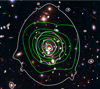
Figure 5.— A three-color HST image of SDSSJ2222 with Swift X-ray contours from the energy range $0.1-2.4$ keV overlaid in green, and the lensing mass contours in white. The red ellipse indicates the statistical uncertainty on the centroid of the main cluster halo component from the lensing analysis (see Section 3 and Table 3). The X-ray emission was smoothed with a Gaussian kernel matching the Swift PSF. Contours are linearly spaced. The thick, horizontal green bar in the upper left-hand corner of the image is $3\farcs 5$ in length, which is size of the astrometric uncertainty.

3. Strong Lensing Analysis

3.1. Multiple images and lensing constraints

The lens model of SDSS J2222$+$2745 relies on observational strong lensing evidence, in the form of multiply-imaged galaxies. The multiband HST images are uniquely useful for the task, owing to their high resolution and broad wavelength coverage that allow identifying multiple images of individual background sources by their color and morphology. In Dahle et al. (2013) we identified six images of one background quasar in imaging data from the Nordic Optical Telescope. We confirmed five of these images and secured their redshift through spectroscopy. The sixth image was predicted by the preliminary lens model and identified in the data after modeling and subtracting the light of the cluster galaxies at the core of the cluster; Dahle et al. (2013) provide strong evidence for the presence of the sixth image. The HST images confirm the sixth image as a counter image of the quasar, with a point-like PSF and similar colors to the other quasar images. These images are labeled A, B, C, D, E, F in Figure 1. A second lensed galaxy A1, at $z=2.3$ (Dahle et al. 2013, Stark et al. 2013), is distorted by the cluster and appears as a blue giant arc south of the cluster center. The new HST data reveal substructure in the giant arc A1, but do not lead to an identification of a counter image of this galaxy. We interpret this giant arc as a likely result of source-plane caustics that bisect the galaxy or pass very close to it, resulting in high magnification in the tangential direction (see Section 4.4).

We identify three secure strongly-lensed galaxies with multiple images in the new HST data.

Source B has three multiple images with unique color, morphological resemblance, and the expected parity. We measure a spectroscopic redshift of $z_{\rm B,spec}=4.56$ using GMOS on Gemini North (see Section 2.2).

Source C is a faint source observed as three images with similar lensing configuration as the three brighter quasar images north of the cluster core. Due to the low surface brightness of C1, C2, and C3, we were not able to obtain a secure spectroscopic redshift. The photometric redshift, spectroscopy, and lensing geometry are all consistent with it being at $z_{\rm C,phot}\sim 3$ (see Section 2.2). We leave the redshift of this source as free parameter in the lensing analysis, with broad priors based on the photometric redshift analysis, $2.0\leq z_{C}\leq 4.0$. We expect that further counter images of this source would be too faint and embedded in the light of the bright cluster galaxies to be detected in the existing data.

Three images of source D appear in the WFC3/IR bands, south of a cluster-member galaxy in the south part of the cluster core. As described in Section 2.2, we were unable to measure a secure spectroscopic redshift for this source. We leave the redshift of this source as free parameter in the lensing analysis, with broad priors based on the photometric redshift analysis, $3.8\leq z_{D}\leq 5.0$.

We identify other candidates of lensed galaxies, however, these are not robustly confirmed as strong lensing features and thus are not used as constraints in the lens model.

We use the positions of the six quasar images, arcs A1, B1-3, C1-3 and D1-3 to constrain the lens model. Resolved emission knots and substructure in the host galaxy of the quasar and B1-3 are also used as additional positional constraints. The redshifts of the quasar and sources A and B are used with no uncertainty, while the redshifts of source C and source D are left as free parameters with broad priors set by the probability distribution functions of their photometric redshifts.

3.2. Strong Lens Model

The lens model is computed using the public software Lenstool (Jullo et al. 2007). Lenstool relies on a ‘parametric’ modeling algorithm, in which the mass distribution is assumed to be a combination of a number of halos, each described by a set of parameters. The software uses Markov Chain Monte Carlo (MCMC) procedure to sample the parameter space, determine the best set of parameters that minimize the scatter between the observed and predicted positions of multiply-imaged lensed galaxies, and determine their uncertainties.

SDSS J2222$+$2745 is modeled with one cluster-scale halo, plus galaxy-scale halos. Each of these halos is modeled as a Pseudo-Isothermal Elliptical Mass Distribution (PIEMD; also known as dual Pseudo Isothermal Elliptical Mass Distribution, Elíasdóttir et al. 2007). The parameters of this mass distribution are positions $x$ and $y$; ellipticity, $e=(a^{2}-b^{2})/(a^{2}+b^{2})$, where $a$ and $b$ are the semi-major and semi-minor axes, respectively; position angle $\theta$, measured north of west; core radius $r_{\rm core}$; cut radius $r_{\rm cut}$; and effective velocity dispersion $\sigma_{0}$. We allow all the parameters of the cluster-scale halos to vary, except for $r_{\rm cut}$, which, for a typical cluster, is much larger than the radius in which lensing evidence can be found and thus cannot be constrained by the model. We fix the cluster-halo $r_{\rm cut}$ at 1500 kpc.

Cluster-member galaxies are selected from a color-magnitude diagram, as those with colors that place them on the cluster red sequence (Gladders & Yee 2000). We note that some galaxies at this redshift may not be quiescent and therefore fall off of this relation. However they are not a dominant component at the core of the cluster (e.g., Fairley et al. 2002). The cluster galaxies are also modeled as PIEMDs, with morphological parameters ($x$, $y$, PA, $\theta$) fixed to their observed values as measured from the HST data in ACS/F814W. $r_{\rm core}$, $r_{\rm cut}$ and $\sigma_{0}$ are assumed to correlate with the luminosity of each galaxy (see Limousin et al. 2005 for a description of the scaling relations).

The slope parameters of five galaxies at the center of the cluster are allowed to deviate from the scaling relation. The lensing potential of the three brightest galaxies near the core of the cluster is responsible for the appearance of the three fainter images of the quasar – D, E, and F. In a close inspection of the galaxies near images D and F, we find that the peak of surface brightness is not aligned with the center of the light distribution of these galaxies, implying a more complex projected mass distribution than that of a single elliptical halo, at least of its stellar mass component. This may be due to the merger history of these galaxies (e.g., Lidman et al. 2013; Lavoie et al. 2016) or a projection effect. We therefore model each of these galaxies as a combination of two halos. One halo has its $x$, $y$ parameters fixed to the center of the extended light distribution of the galaxy, its ellipticity and position angle follow those of the light distribution, and the other parameters allowed to vary. The second halo is centered on the peak surface brightness, with circular symmetry, vanishing core radius, and $\sigma_{0}$ and $r_{cut}$ set as free parameters.

The distribution of the intracluster light is observed to by more extended in the North-South direction (Figure 1), which would be consistent with a young dynamical age for the cluster. However, the deep combined NOT and Gemini images (Dahle et al. 2015) indicate considerable Galactic cirrus in the field, which is difficult to disentangle from intracluster light at the very faintest surface brightness levels.

Although we find that some of the free parameters are not sensitive to the positional lensing constraints, we allow these parameters to vary in order to encompass the full range of statistical uncertainties, and investigate their affect on the time delay of the quasar images.

In Table 3, we list the lens model parameters and their uncertainties, including the time delay constraints (95% confidence limit from Dahle et al. 2015). We plot the critical curves from the best-fit model in Figure 6, for a source at $z=$2.805. The best-fit model has an image-plane RMS of $0\farcs 16$. We note that since the RMS was computed from the predicted positions of the same images that were used as constraints, it is not an unbiased indicator of the model fidelity (Johnson & Sharon 2016).

The time delay between the images of the quasar can be measured from the arrival time surface (e.g., Schneider 1985),

$$\tau(\vec{\theta},\vec{\beta})=\frac{1+z_{l}}{c}\frac{D_{l}D_{s}}{D_{ls}}\bigg{[}\frac{1}{2}(\vec{\theta}-\vec{\beta})^{2}-\psi(\vec{\theta})\bigg{]},$$ (1)

where $\vec{\beta}$ is the source location, $\vec{\theta}$ is a coordinate in the image plane, $z_{l}$ is the lens redshift, $D_{l}$ and $D_{s}$ are the distances from the observer to the lens and to the source, respectively, $D_{ls}$ is the distance from the lens to the source, and $\psi$ is the lensing potential. Figure 7a shows the Fermat potential of the best-fit model, with the positions of the observed quasar images overplotted. Multiple images occur in stationary points in this potential, i.e., maxima, minima, and saddle points. The lens model successfully predicts the formation of all the observed quasar image as well as three additional demagnified images, each within $0\farcs 1$ of the center of galaxies G1, G2, and G3, at the extrema points of the Fermat potential. However, these images are predicted to be several magnitudes fainter than the faintest observed image of the quasar, with $29-34$ mag in the F435W band, and thus we do not expect to be able to detect them in the current data.

We report the predicted arrival time in days relative to image A of the quasar, $\Delta t=\tau(\vec{\theta},\vec{\beta})-\tau(\vec{\theta}_{\textrm{A}},\vec{\beta})$. As can be seen in Equation 1, the Fermat potential depends on the source position, $\vec{\beta}$. It is in fact very sensitive to small changes in the exact value of $\vec{\beta}$. We therefore follow the procedure described in Sharon & Johnson (2015), and take the source plane scatter into account when computing the uncertainties of the time delay of the quasar images. The best-fit time delays and their uncertainties are listed in Table 4.

Time delays are not implemented as constraints at this point. We derive a lens model with no prior on the time delays, and later confront the model with the measured time delays from Dahle et al. (2015) in a posterior analysis – see Section 4.1. After applying the observational time delay constraints on the posterior distribution, we find that parts of the parameter space are excluded.

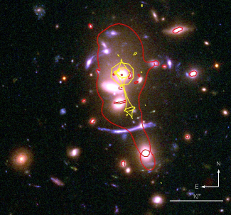
Figure 6.— The critical curves for a source at $z=2.805$ from our best-fit lens model are over-plotted on a color-composite HST image of SDSS J2222$+$2745.

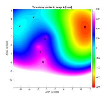
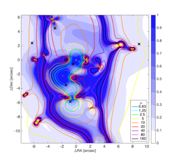
Figure 7.— (a) Left: Excess arrival time surface (Fermat potential) for light emitted from the source position in the source plane at $z=$2.805, and traverses the lens plane at $z=$0.49. The best-fit model, from which we compute this time surface, takes into account the 95% confidence interval of the measred time delays from Dahle et al. (2015). The excess arrival time is computed relative to image A of the quasar, and given in days. (b) Right: The magnification map of a source at $z=$2.805 from the best-fit model is shown in contours. The colormap background gives the relative uncertainty in each point, $\Delta\mu/\mu$. In both panels, the positions of the six images of the quasar are marked, and coordinates are indicated in arcsec relative to [RA, Dec]=[335.535745, 27.7598861].

Table 3Best-fit lens model parameters

No.	Component	$\Delta$ RA ($\arcsec$)	$\Delta$ Dec ($\arcsec$)	$e$	$\theta$ (deg)	$r_{\rm core}$ (kpc)	$r_{\rm cut}$ (kpc)	$\sigma_{0}$ (km s-1)
1	Cluster halo	$0.26\pm 0.22$	$2.53\pm 1.20$	$0.29\pm 0.05$	$95.8\pm 2.1$	$42.7\pm 6.5$	[$1500$]	$668\pm 22$
2	G1 halo	[$0.029$]	[$0.036$]	[$0.062$]	[$24.3$]	$0.13\pm 0.13$	$24.9\pm 23.5$	$274\pm 85$
3	G1 core	[$0$]	[$0$]	[$0$]	[$0$]	[$0.001$]	$23.6\pm 23.2$	$30.3\pm 19.5$
4	G2 halo	[$1.895$]	[$-2.351$]	[$0.669$]	[$-15.6$]	$0.15\pm 0.13$	$11.0\pm 8.3$	$294\pm 104$
5	G2 core	[$1.895$]	[$-2.347$]	[$0$]	[$0$]	[$0.001$]	$24.9\pm 20.9$	$29.2\pm 18.8$
6	G3 halo	[$0.583$]	[$-5.339$]	[$0.222$]	[$51.1$]	$0.16\pm 0.13$	$27.7\pm 22.3$	$209\pm 28$
7	G3 core	[$0.583$]	[$-5.339$]	[$0$]	[$0$]	[$0.001$]	$26.7\pm 22.8$	$32.2\pm 17.5$
8	G4	[$-4.425$]	[$-14.789$]	$0.49\pm 0.20$	$-74.7\pm 3.9$	$3.56\pm 1.32$	$18.5\pm 14.6$	$360\pm 129$
9	G5	[$3.35$]	[$5.605$]	$0.66\pm 0.13$	$-60.0\pm 9.7$	[$0.043$]	[$7.213$]	$56.2\pm 43.2$
	L* galaxy	$\cdots$	$\cdots$	$\cdots$	$\cdots$	[0.15]	[50]	[130]

Note. — The coordinates are given in arcseconds measured East and North of the core of galaxy G1, at [RA, Dec]=[335.535745, 27.7598861]. All the mass components are parameterized as PIEMD, with ellipticity expressed as $e=(a^{2}-b^{2})/(a^{2}+b^{2})$. $\theta$ is measured North of West. Error bars are inferred from the MCMC optimization and correspond to 1$\sigma$. Parameters that were not optimized are listed in square brackets. The location and the ellipticity of the matter clumps associated with cluster galaxies were kept fixed according to their light distribution, and the other parameters determined through scaling relations (see text).

4. Results and Discussion

4.1. Time Delays

Observational measurement of the time delays between the images of the quasar can provide valuable constraints on the lens model, as the arrival time is sensitive to the lensing potential. SDSS J2222$+$2745 gives us a unique opportunity to obtain observational constraints on the time delay from six images of the same background quasar, three of which appear close to the cluster core, in close proximity to cluster galaxies. In Dahle et al. (2015) we report on the measurement of time delays between the three bright images of the quasar, $\tau_{\rm AB}$=$47.7\pm{6.0}$ days, and $\tau_{\rm AC}$=$-722\pm{24}$ days (all the time delays are measured as excess arrival time relative to image A of the quasar). Our basic lensing analysis does not use the time delays as constraints, and is done strictly without any a priori knowledge of the time delays.

We now confront the lens model with the time delay observations. The basic lensing analysis predicts that the arrival time is shortest for image C of the quasar, followed by images A,B,F,D,E. Quantitatively, we find $\tau_{\rm AB}$=$47\pm{20}$ days, and $\tau_{\rm AC}$=$-726\pm{294}$ days, in good agreement with the observed measurements of Dahle et al. (2015).

Next, we use the observed time constraints and their 95% confidence limits to further constrain the parameter space. We select the sets of parameters from the MCMC sampling that result in lens models with $\chi^{2}$ in the range [$\chi^{2}$,$\chi^{2}+4.5$]. We consider these models as producing reasonable scatter in the predicted vs. observed positions of images of the lensed galaxies, and their parameters are drawn from a range larger than the 1$\sigma$ confidence interval of the parameter space of well-constrained parameters, as sampled by the MCMC process. Models with larger $\chi^{2}$ were rejected. We then compute the Fermat potential for each one of these sets of parameters (Equation 1), assuming that the quasar source position $\vec{\beta}$ is at the mean of the predicted source positions of the six quasar images. We compute the excess arrival time relative to image A of the quasar, i.e., the predicted time delay for each of the images. We identify the models that predict time delays $\tau_{\rm AB}$  and $\tau_{\rm AC}$ within the 95% confidence limit of the observed values of Dahle et al. (2015). In Figure 8, we plot the positional $\chi^{2}$ against each of the parameters of the main cluster halo, and color-code the models that predict either $\tau_{\rm AB}$ in the range $47.7\pm{6.0}$ days, $\tau_{\rm AC}$ in the range $-722\pm{24}$ days, or both. As can be seen in Figure 8, while models that predict the observed $\tau_{\rm AB}$ span the entire parameter space, the measured time delay between image C and A, $\tau_{\rm AC}$, has good constraining power over some of the parameters, mainly the overall mass of the main cluster halo ($\sigma_{0}$), and its ellipticity ($e$).

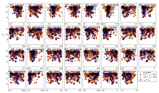
Figure 8.— The goodness of fit plotted against the parameter value, for sets of parameters from the MCMC analysis. The goodness of fit is estimated via the $\chi^{2}$ value, computed by Lenstool as the scatter between observed and predicted image positions. Models that predict $\tau_{\rm AB}$ in the range $47.7\pm{6.0}$ days are plotted in red squares; models that predict $\tau_{\rm AC}$ in the range $-722\pm{24}$ days are plotted in green circles; models that satisfy both criteria are circled in black. All other models are plotted in gray circles. The observed time delay $\tau_{\rm AC}$ has constraining power over the parameters of the main cluster halo, mainly the normalization $\sigma_{0}$, which is correlated with the overall mass of the cluster, and the ellipticity $e$.

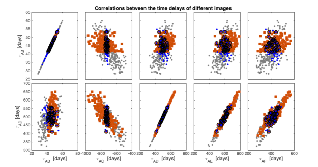
Figure 9.— Correlations between the predicted relative time delays of the six quasars. The top and bottom rows show $\tau_{\rm AB}$ and $\tau_{\rm AD}$  respectively, plotted against the other relative time delays. Colors and symbols are the same as in Figure 8. We see correlation between all the relative time delays except for $\tau_{\rm AB}$. Thus the observational measurements of $\tau_{\rm AB}$ and $\tau_{\rm AC}$ (Dahle et al. 2015) have strong constraining power over the model. Furthermore, observational measurement of either of the A-D,E,F time delays will narrow the uncertainty on the predicted time delays of the other images.

We find strong correlation between the predicted time delays $\tau_{\rm AD}$, $\tau_{\rm AE}$, and $\tau_{\rm AF}$, as can be seen in Figure 9. Interestingly, $\tau_{\rm AD}$, $\tau_{\rm AE}$, and $\tau_{\rm AF}$ do not correlate with $\tau_{\rm AB}$, but they have strong correlation with $\tau_{\rm AC}$. This correlation places a tight constraint on the predicted time delays of the three central images. Moreover, the arrival times of images D, E, and F are strongly correlated, which means that a time delay measurement of one of them will provide an additional strict constraint on the time delays of the other images.

The correlation of the time delays of the central images is not surprising. The arrival time lag of the central images is dominated by gravitational time delay as the light travels close to the center of mass, due to the deep potential well of the cluster; light will take longer to travel on this path, although this path is geometrically shorter (with smaller impact parameter and smaller deflection). Thus $\tau_{\rm AC}$ is linked to $\tau_{\rm AD}$, $\tau_{\rm AE}$, $\tau_{\rm AF}$  through its correlation with the overall normalization of the cluster halo, i.e., the effective velocity dispersion, $\sigma_{0}$.

Applying the time delay observational cut on the parameter space, we are able to narrow down the uncertainties on the predicted time delays of the central images. Interestingly, we find that these time delays are short enough to be measured within the next few years: $\tau_{\rm AD}=$$502\pm{68}$, $\tau_{\rm AE}=$$611\pm{75}$, and $\tau_{\rm AF}=$$415\pm{72}$ days; Moreover, the arrival time of E and F relative to D is short – of order 3-5 months: $\tau_{DE}=$$102\pm{23}$, $\tau_{DF}=$$-85\pm{39}$ days, thus measuring $\tau_{\rm DE}$ and $\tau_{\rm DF}$ can be achieved within a year or two of cadenced imaging with a large telescope (Section 5).

In the following sections, the results of the lensing analysis take into account the constraints from the observed time delays, as measured by Dahle et al. (2015), and their 95% confidence interval as described above.

4.2. Cluster Mass

We report the lensing-inferred total projected mass density of the lens (cylindrical mass) within projected radii of 100, 200, and 500 pc: $M_{(<100{\rm kpc})}$ = $0.55\pm 0.03\times 10^{14}$ M_⊙, $M_{(<200{\rm kpc})}$ = $1.15\pm 0.1\times 10^{14}$ M_⊙, and $M_{(<500{\rm kpc})}$ = $2.50\pm 0.24\times 10^{14}$ M_⊙, $\pm 10\%$ systematic uncertainty. The statistical uncertainties are derived from the MCMC sampling of the parameter space, combined with the Dahle et al. (2015) 95% confidence interval of the time delay measurements (see Section 4.1). An additional 10% systematic uncertainty should be applied, given the relatively small number of constraints and spectroscopic redshifts, that limit the accuracy of the lens model. Johnson & Sharon (2016) found that while the enclosed mass is well constrained at the radius of the lensing evidence, its systematic uncertainty decreases with increasing number of lensing constraints and spectroscopic redshifts. The analysis in Johnson & Sharon (2016) is tuned to the typical number of constraints in high cross-section lensing clusters such as the Frontier Fields (Lotz et al. 2016), and therefore they do not sample the affect on systematics in a case like SDSS J2222$+$2745, a much lower-mass cluster with four multiply-imaged lensed sources and three spectroscopic redshifts. We therefore conservatively adopt a $10\%$ systematic uncertainty on the enclosed mass, which is the typical uncertainty for a case of five sources and no spectroscopic redshifts. Interestingly, the observational measurement of the $\tau_{\rm AC}$ time delay places a tight constraint on the total enclosed mass and is what drives the relatively small statistical uncertainty.

Figure 5 shows the contours of the projected mass density distribution from the strong lens model, and the X-ray contours from Swift observations (Section 2.3). We find that the X-ray emitting gas and the dark matter distribution are generally aligned, with no significant offset between their centroids. A more robust measurement of the X-ray distribution will be enabled with the superior resolution of Chandra observations.

4.3. Magnification

The magnification map for a source at the quasar redshift, $z=2.805$, and the magnifications measured at the position of each image of the quasar, are shown in Figure 7b and Table 4, respectively. The uncertainties are estimated by computing magnification maps for a series of lens models sampled from steps the MCMC that correspond to $1\sigma$ in the parameter space, and the 95% confidence interval of the time delay measuremens of Dahle et al. (2015). Since quasars are variable sources and are not standard candles, we cannot compare the absolute predicted lensing magnification with an observational measurement. Nevertheless, we can compare the predictions to the relative magnifications between images A, B, and C of the quasar, for which time delays have been measured. Dahle et al. (2015) find that the light curves of images A, B, and C, can be matched with time delays of $\tau_{\rm AB}$=$47.7\pm{6.0}$ and $\tau_{\rm AC}$=$-722\pm{24}$, and magnitude shift of $\Delta m_{\rm AB}=0.340\pm 0.007$ mag and $\Delta m_{\rm AC}=0.483\pm 0.012$ mag. We find that the model is in agreement with the observed relative magnification of image A and B. The model-predicted magnification of C is $\sim 30\%$ too high to agree with the observed magnification ratio between A and C, indicating that the systematic uncertainties may be underestimated. We note that substructure in the cluster, as well as structure along the line of sight, may contribute to discrepancy between the measured and model-derived relative magnifications.

Compared to the initial model in Dahle et al. (2013), which was based on ground-based observations, we find that the magnifications of A, B, and C are $\sim 2.5\times$ higher than those derived in Dahle et al. (2013), but well within the large statistical uncertainties reported there. Moreover, systematic uncertainties, which are not taken into consideration, are large for lens models that are based on few lensed sources and few spectroscopic redshifts (Johnson & Sharon 2016). We also note that the new constraints from the HST data required a more massive component at the south of the cluster (G4) to explain the lensing evidence that was not identified from the ground. Compared to the magnifications in other wide-separation lensed quasars, we find that the magnifications of A, B, and C in SDSS J2222$+$2745 are similar to the best-fit model-predicted magnifications of the three brightest images in SDSSJ1029, from Oguri et al. (2013), while in Oguri et al. (2010), the lens model of SDSSJ1004 predicts magnifications a factor $\sim 2\times$ higher.

Table 4Model-predicted magnifications and time delays

Image	F435W	Magnification		Time delay
	magnitude	$\mu$		[days]
A	21.861	$14.5\pm 2.7$	$\cdots$	$\cdots$
B	22.261	$10.8\pm 4.3$	$\tau_{\rm AB}$	[ $47.7\pm{6.0}$]
C	22.227	$6.7\pm 1.0$	$\tau_{\rm AC}$	[$-722\pm{24}$]
D	23.827	$1.43\pm 0.75$	$\tau_{\rm AD}$	$502\pm{68}$
E	24.070	$0.76\pm 0.39$	$\tau_{\rm AE}$	$611\pm{75}$
F	24.909	$0.95\pm 0.65$	$\tau_{\rm AF}$	$415\pm{72}$

Note. — Magnitudes in the ACS/F435W filter are measured within an aperture of radius $0\farcs 56$ in an observation starting on JD 2456941.06751. Time delay is given in days, relative to image A. $\tau_{\rm AB}$ and $\tau_{\rm AC}$ are observational constraints from Dahle et al. (2015). The uncertainties represent the 95% confidence level from the combined MCMC analysis and the observational time delay constraints.

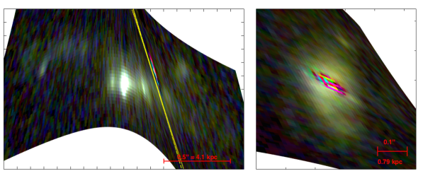
Figure 10.— Source plane reconstruction of galaxy A1 at $z=$2.3 (left) and of the quasar host galaxy at $z=$2.805 (right). The quasar host is generated from image A of the quasar. The foreground white dwarf and the point-source emission from the quasar are masked to reveal the underlying information (see text). A horizontal bar indicates the scale in arcseconds and kpc at each source redshift. The yellow lines in the left panel are the locations of the source plane caustics, which map to the critical curves in the image plane.

4.4. Source Plane Reconstruction

We reconstruct the source image of the lensed galaxy A1 at $z=$2.3, and the host galaxy of the quasar at $z=$2.805, by ray-tracing the image-plane pixels through the lens equation, $\vec{\beta}=\vec{\theta}-\vec{\alpha}(\vec{\theta})$, where $\vec{\beta}$ is the source position of each pixel, $\vec{\theta}$ is its observed position, and $\vec{\alpha}(\vec{\theta})$ is the deflection matrix scaled by $d_{LS}/d_{S}$, the ratio between the distance from the lens to the source and from the observer to the source. The high lensing magnification resolves small substructure in these galaxies, which would otherwise be too small for HST resolution. Galaxy A1 is highly distorted by the lensing potential due to its close proximity to the caustic. It is likely that a small region of this galaxy is multiply imaged within the giant arc.

Prior to ray tracing the images, we subtract the light of the point source quasar light and the foreground white dwarf to reveal the underlying information. In each band we select a star in the field of view with similar brightness. We generate a second image by shifting the data so that the star is at the exact pixel position of the point source we wish to mask. We then scale the shifted image and subtract it from our data. Figure 10 shows the reconstructed source-plane image of galaxy A, and of the quasar host galaxy.

From the reconstructed source image, A1 measures $\sim 13$ kpc in diameter and the quasar host is measured to be $\sim 3$ kpc in diameter. A thorough investigation of the physical properties of these galaxies is left for future work.

4.5. Absorbing Systems

Stark et al. (2013) find strong evidence for an absorption system at $z=$2.3 in the spectrum of image A of the quasar, indicating that the extended gas halo of galaxy A1 has neutral hydrogen and metals, from absorption lines of Ly$\alpha$, Si II $\lambda 1526$ and CIV $\lambda 1549$. Stark et al. (2013) estimate the projected distance between A1 and image A of the quasar at $\sim 50$ kpc.

A proper estimate of the impact parameter takes into account the path of the light from the quasar source plane to each of its images, and where these paths traverse the source plane of A1, at $z=$2.3. In the left panel of Figure 11 we show a reconstruction of the source plane at the redshift of galaxy A1. By ray-tracing the quasar images to the same redshift of A1, we find that the quasar light passes 34 kpc north of the center of A1. At this redshift, the quasar paths are separated by as much as 5 kpc. We are therefore presented with a unique opportunity to sample the uniformity of the gas halo on scales of a few kpc, with at least three bright lines of sight.

Our GMOS multi-object spectroscopy masks targeted images A, B, C, and D of the quasar. Slits were placed on these sources on both nod and shuffle positions, and on both masks, resulting in a total of 2400 s on target for A, B, D, and 3600 s on target for C. The wavelength coverage allows the detection of FeII 2586,2600 and MgII 2796,2803 at the redshift of A1.

The intervening absorption system is detected in the spectra of all three bright images of the quasar (A, B, C), at a redshift of $z=2.2988\pm 0.0002$. In the right panel of Figure 11, we plot the two strongest features of this system, the Mg II 2796,2803 Å doublet and the Fe II 2600 Å line. The spectra were continuum normalized, with the continuum calculated by smoothing the spectra with a 40 Å boxcar.

In Table 5 we tabulate the equivalent width and redshift measurements for this absorption system in each quasar spectrum. Since the blue wing of the Mg II 2976 Å feature is affected by the [Ne IV] and Fe III emission complex at 2423 Å rest-frame (Vanden Berk et al., 2001), we do not try to fit this line, but instead consider the weaker transition Mg II 2803.

The intervening system is clearly detected in Mg II in all three images of the quasar; the weaker Fe II 2600 is detected in quasar images A and B. The equivalent widths are comparable given the uncertainties listed in Table 5. While Figure 11 shows some variation in the absorption profiles from quasar image to image, particularly in the amount of redshifted absorption, these variations may not be significant given the signal-to-noise ratio of the data. Deeper spectra are required to measured differences in the absorption along these three lines of sight.

We also detect FeII and MgII absorption from a second absorber at z=1.202 in the three spectra. The corresponding object is not currently identified in the imaging or spectroscopic data. The largest separation between the quasar lines of sight at this redshift is $\sim$40 kpc.

Co-adding the spectra from the forthcoming spectroscopic followup campaign (Section 5) will result in a deep spectrum of each of the quasar images, and high enough signal to noise to determine some of the physical properties of the gas halo in the absorbing systems.

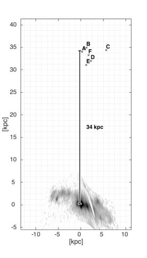
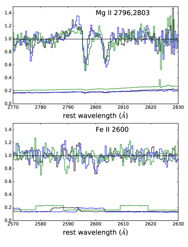
Figure 11.— Left: The $z=2.3$ plane, reconstructed from our lens model. At this redshift plane, the light from the $z=$2.805 quasar passes $\sim 34$ kpc from galaxy A; the separation between the light rays of the quasar is a few kpc. The extended gas halo around galaxy A is seen in absorption in the spectra of the quasar, which permits a study of the spatial distribution of the physical properties of the gas. The grid is given in kpc, centered on the brightness peak of galaxy A. Right: Continuum-normalized spectra of the intervening absorption system at $z=2.2988\pm 0.0002$, for quasar spectra A (plotted in black), B (blue), and C (green). The Mg II 2796, 2803 doublet and the Fe II 2600 transition are shown at the top and bottom panels, respectively. The intervening absorber is clearly detected in Mg II in all three quasar spectra, and in Fe II in quasar images A and B.

5. Future Work

Ongoing monitoring with the Nordic Optical Telescope (PI: Dahle) will tighten the constraints on the measured time delays. Recent observations indicate that image C of the quasar continues its brightening trend, and the measured 722 day lag provides a unique opportunity to plan future observations of A and B when they are at their brightest epoch. During the 2018 observing season, images A and B will both reach a level $>$1.1 magnitudes brighter than during the GMOS spectroscopic observations reported in this paper. Imaging monitoring with Gemini North (GN-2016A-Q-28; PI: Gladders) is under way to constrain the time delays between the internal three images (D, E, F) of SDSS J2222$+$2745. Spectroscopic monitoring with Gemini North (GN-2016B-Q-28; PI: Treu) will enable a measurement of the mass of the central black hole through reverberation mapping (Blandford & McKee 1982; Peterson 1993; Pancoast, Brewer & Treu 2011). In this paper, we present a revised lens model of SDSS J2222$+$2745 from high resolution multiband HST imaging, new spectroscopic redshifts, and constraints from the measured time delays of three images of the background quasar. The astrophysical applications of SDSS J2222$+$2745 span from studies of galaxy structure at small physical scales, quasar physics, cluster astrophysics and cosmology; its investigation has just begun.

Table 5Equivalent width and redshift measurements for the intervening absorption system

spectrum	EW_r(Å) $\pm\sigma$	redshift
Mg II 2803 Å
QSO-A	$-0.14\pm 0.09$	2.2986
QSO-B	$-0.26\pm 0.09$	2.2990
QSO-C	$-0.23\pm 0.1$	2.2989
mean	$-0.21\pm 0.05$	2.2988
Fe II 2600 Å
QSO-A	$-0.14\pm 0.06$	2.2981
QSO-B	$-0.13\pm 0.08$	2.2987
QSO-C	$-0.04\pm 0.07$	2.2998
mean	$-0.10\pm 0.05$	2.2989

Note. — Measured equivalent widths and redshifts for the strongest absorption lines in the intervening absorber. Equivalent widths are in the rest-frame, in Å, and are determined by direct summation. Redshifts are taken from the most absorbed pixel for individual quasar spectra. For each absorption line, we quote the mean of the measurements across all three quasar spectra.

References

- Aihara et al. (2011) Aihara, H., Allende Prieto, C., An, D., et al. 2011, ApJS, 193, 29
- Arnaud (1996) Arnaud, K. A. 1996, Astronomical Data Analysis Software and Systems V, 101, 17
- Bayliss et al. (2011a) Bayliss, M. B., Hennawi, J. F., Gladders, M. D., et al. 2011, ApJS, 193, 8
- Bayliss et al. (2011b) Bayliss, M. B., Gladders, M. D., Oguri, M., et al. 2011, ApJ, 727, L26
- Bayliss et al. (2014) Bayliss, M. B., Johnson, T., Gladders, M. D., Sharon, K., & Oguri, M. 2014, ApJ, 783, 41
- Beers et al. (1990) Beers, T. C., Flynn, K., & Gebhardt, K. 1990, AJ, 100, 32
- Blandford & McKee (1982) Blandford, R. D., & McKee, C. F. 1982, ApJ, 255, 419
- Brammer et al. (2008) Brammer, G. B., van Dokkum, P. G., & Coppi, P. 2008, ApJ, 686, 1503-1513
- Dahle et al. (2013) Dahle, H., Gladders, M. D., Sharon, K., et al. 2013, ApJ, 773, 146
- Dahle et al. (2015) Dahle, H., Gladders, M. D., Sharon, K., Bayliss, M. B., & Rigby, J. R. 2015, ApJ, 813, 67
- Elíasdóttir et al. (2007) Elíasdóttir, Á., Limousin, M., Richard, J., et al. 2007, arXiv:0710.5636
- Evans et al. (2014) Evans, P. A., Osborne, J. P., Beardmore, A. P., et al. 2014, ApJS, 210, 8
- Evrard et al. (2008) Evrard, A. E., Bialek, J., Busha, M., et al. 2008, ApJ, 672, 122-137
- Fairley et al. (2002) Fairley, B. W., Jones, L. R., Wake, D. A., et al. 2002, MNRAS, 330, 755
- Gladders & Yee (2000) Gladders, M. D., & Yee, H. K. C. 2000, AJ, 120, 2148
- Gonzaga & et al. (2012) Gonzaga, S., & et al. 2012, The DrizzlePac Handbook, HST Data Handbook,
- Hennawi et al. (2008) Hennawi, J. F., Gladders, M. D., Oguri, M., et al. 2008, AJ, 135, 664
- Hook et al. (2004) Hook, I. M., Jørgensen, I., Allington-Smith, J. R., et al. 2004, PASP, 116, 425
- Inada et al. (2006) Inada, N., Oguri, M., Morokuma, T., et al. 2006, ApJ, 653, L97
- Inada et al. (2003) Inada, N., Oguri, M., Pindor, B., et al. 2003, Nature, 426, 810
- Johnson & Sharon (2016) Johnson, T. L. & Sharon, K. 2016, ApJsubmitted
- Jullo et al. (2007) Jullo, E., Kneib, J.-P., Limousin, M., Elíasdóttir, Á., Marshall, P. J., & Verdugo, T. 2007, New Journal of Physics, 9, 447
- Kalberla et al. (2005) Kalberla, P. M. W., Burton, W. B., Hartmann, D., et al. 2005, A&A, 440, 775
- Lavoie et al. (2016) Lavoie, S., Willis, J. P., Démoclès, J., et al. 2016, MNRAS,
- Lidman et al. (2013) Lidman, C., Iacobuta, G., Bauer, A. E., et al. 2013, MNRAS, 433, 825
- Limousin et al. (2005) Limousin, M., Kneib, J.-P., & Natarajan, P. 2005, MNRAS, 356, 309 2001, ApJ, 563, 9
- Lotz et al. (2016) Lotz, J. M., Koekemoer, A., Coe, D., et al. 2016, arXiv:1605.06567
- Mantz et al. (2010) Mantz, A., Allen, S. W., Ebeling, H., Rapetti, D., & Drlica-Wagner, A. 2010, MNRAS, 406, 1773
- Ofek (2014) Ofek, E. O. 2014, Astrophysics Source Code Library, 1407.005
- Oguri (2010) Oguri, M. 2010, PASJ, 62, 1017
- Oguri et al. (2013) Oguri, M., Schrabback, T., Jullo, E., et al. 2013, MNRAS, 429, 482
- Pancoast et al. (2011) Pancoast, A., Brewer, B. J., & Treu, T. 2011, ApJ, 730, 139
- Peterson (1993) Peterson, B. M. 1993, PASP, 105, 247
- Rajan & et al. (2011) Rajan, A., & et al. 2011, WFC3 Data Handbook, HST Data Handbooks,
- Ruel et al. (2014) Ruel, J., Bazin, G., Bayliss, M., et al. 2014, ApJ, 792, 45
- Shapley et al. (2003) Shapley, A. E., Steidel, C. C., Pettini, M., & Adelberger, K. L. 2003, ApJ, 588, 65
- Sharon et al. (2014) Sharon, K., Gladders, M. D., Rigby, J. R., et al. 2014, ApJ, 795, 50
- Sharon & Johnson (2015) Sharon, K., & Johnson, T. L. 2015, ApJ, 800, L26
- Skelton et al. (2014) Skelton, R. E., Whitaker, K. E., Momcheva, I. G., et al. 2014, ApJS, 214, 24
- Smith et al. (2009) Smith, G. P., Ebeling, H., Limousin, M., et al. 2009, ApJ, 707, L163
- Stark et al. (2013) Stark, D. P., Auger, M., Belokurov, V., et al. 2013, MNRAS, 436, 1040
- Vanden Berk et al. (2001) Vanden Berk, D. E., Richards, G. T., Bauer, A., et al. 2001, AJ, 122, 549
- Xue & Wu (2000) Xue, Y.-J., & Wu, X.-P. 2000, ApJ, 538, 65
- York et al. (2000) York, D. G., Adelman, J., Anderson, J. E., Jr., et al. 2000, AJ, 120, 1579