Analysis of Carrier’s problem

Abstract

A computational and asymptotic analysis of the solutions of Carrier’s problem is presented. The computations reveal a striking and beautiful bifurcation diagram, with an infinite sequence of alternating pitchfork and fold bifurcations as the bifurcation parameter tends to zero. The method of Kuzmak is then applied to construct asymptotic solutions to the problem. This asymptotic approach explains the bifurcation structure identified numerically, and its predictions of the bifurcation points are in excellent agreement with the numerical results. The analysis yields a novel and complete taxonomy of the solutions to the problem, and demonstrates that a claim of Bender & Orszag [3] is incorrect.

1 Introduction

In 1970, G. F. Carrier [5, eq. (3.5)] introduced the following singular perturbation problem

$$\epsilon^{2}y^{\prime\prime}+2(1-x^{2})y+y^{2}=1,\qquad y(-1)=y(1)=0,$$ (1)

where $0<\epsilon\ll 1$, and a prime represents $\mathchoice{\frac{\mathrm{d}}{\mathrm{d}x}}{\mathrm{d}/\mathrm{d}x}{\mathrm{d}/\mathrm{d}x}{\mathrm{d}/\mathrm{d}x}$. This remarkably beautiful and complex problem is discussed in more detail in the textbooks of Carrier & Pearson [6, p. 197] and Bender & Orszag [3, p. 464]. We briefly review their discussion.

Since (1) is singularly perturbed, we expect the solution to comprise an outer solution valid for $1-|x|\gg\epsilon$ combined with possible boundary layers near $x=\pm 1$. Naïvely setting $\epsilon=0$ gives the leading-order outer solution as

$$y_{\mathrm{out}}=x^{2}-1\pm\sqrt{1+(1-x^{2})^{2}}.$$ (2)

For neither choice of sign does $y_{\mathrm{out}}$ satisfy the boundary conditions at $x=\pm 1$, so there are indeed boundary layers. In the boundary layer near $x=-1$ we set $x=-1+\epsilon X$, $y(x)=y_{\mathrm{in}}(X)$ to give

$$\mathchoice{\frac{\mathrm{d}^{2}y_{\mathrm{in}}}{\mathrm{d}X^{2}}}{\mathrm{d}^{2}y_{\mathrm{in}}/\mathrm{d}X^{2}}{\mathrm{d}^{2}y_{\mathrm{in}}/\mathrm{d}X^{2}}{\mathrm{d}^{2}y_{\mathrm{in}}/\mathrm{d}X^{2}}+y_{\mathrm{in}}^{2}=1,\qquad y_{\mathrm{in}}(0)=0.$$ (3)

In order to match with the outer solution, $y_{\mathrm{in}}$ must tend to $\pm 1$ as $X\rightarrow\infty$. Bender & Orszag show that there are no solutions tending to $1$, so that the minus sign must be chosen in the outer approximation (2). On the other hand, there are two solutions of (3) which tend to $-1$ at infinity, namely

$$y_{\mathrm{in}}=-1+3\,\mathrm{sech}^{2}\left(\pm\frac{X}{\sqrt{2}}+\tanh^{-1}\left(\sqrt{\frac{2}{3}}\right)\right).$$ (4)

Similarly there are two possible boundary layer solutions near $x=1$. Thus it seems that a matched asymptotic analysis has produced four independent solutions of the equation. As Bender & Orszag say, “it is a glorious triumph of boundary layer theory that all four solutions actually exist and are extremely well approximated by the leading-order uniform approximation” generated from (2) and (4). These uniform approximations are shown in Figure 1.

Fig. 1: The four asymptotic solutions with $\epsilon^{2}=0.00223$, generated using the outer approximation (2) and the boundary layer approximations (4).

However, the story does not end there. Bender & Orszag show that it is also possible to have a solution with an internal layer near $x=0$. Writing $x=\epsilon X$, $y(x)=y_{\mathrm{in}}(X)$ gives

$$\mathchoice{\frac{\mathrm{d}^{2}y_{\mathrm{in}}}{\mathrm{d}X^{2}}}{\mathrm{d}^{2}y_{\mathrm{in}}/\mathrm{d}X^{2}}{\mathrm{d}^{2}y_{\mathrm{in}}/\mathrm{d}X^{2}}{\mathrm{d}^{2}y_{\mathrm{in}}/\mathrm{d}X^{2}}+2y_{\mathrm{in}}+y_{\mathrm{in}}^{2}=1,$$ (5)

with the spike solution

$$y_{\mathrm{in}}=3\sqrt{2}\,\mathrm{sech}^{2}(2^{-1/4}X+A)-1-\sqrt{2},$$ (6)

where we have matched with the outer solution by requiring that $y_{\mathrm{in}}\rightarrow-1-\sqrt{2}$ as $|X|\rightarrow\infty$. The constant $A$ (corresponding to a translation in the centre of the spike) is left undetermined in [3], although it is shown in [15] that it must be zero. Since this internal spike solution can be combined with any combination of boundary layers at $x=\pm 1$, we have generated another four solutions to (1).

One might ask whether it is possible to have more than one internal spike. Bender & Orszag claim that “for a given positive value of $\epsilon$ there are $4(N+1)$ solutions to (1) which have from 0 to $N$ internal boundary layers at definite locations, where $N$ is a finite number depending on $\epsilon$”.

There seems to have been remarkably little work following up on this claim. MacGillivray et al. [15] considered the solutions with two spikes in detail. They showed that the spikes must be symmetrically placed about $x=0$, and that the separation between them is $O(\epsilon\log\epsilon)$. In view of the rather intricate asymptotic analysis in [15], it is perhaps not surprising that no attempt has been made to analyze the three spike solutions.

On the other hand, the asymptotic dependence of the maximum number of spikes $M_{\rm max}$ on $\epsilon$ has been determined. Ai [1] showed that $M_{\rm max}$ is $O(1/\epsilon)$, and subsequently Wong and Zhao [17] showed that

$$M_{\rm max}\sim\left\lfloor\frac{K}{\epsilon}\right\rfloor,$$

where $K\approx 0.4725$ and $\lfloor x\rfloor$ is the greatest integer less than or equal to $x$. Wong and Zhao also showed that the number of solutions of (1) is between $4M_{\rm max}-3$ and $4M_{\rm max}$.

We also note that Kath has developed a general method which gives a qualitative understanding of the number and type of solutions to equations such as (1) in terms of slowly varying phase planes [10]. Kath’s conclusions are similar to those of Bender and Orszag.

In this paper we investigate the claim of Bender & Orszag, both numerically and asymptotically.

We first apply a powerful new algorithm for computing bifurcation diagrams, deflated continuation [9], to Carrier’s problem. This computation reveals a striking and intricate bifurcation diagram, with new solutions coming into existence via an apparently infinite sequence of alternating pitchfork and fold bifurcations as $\epsilon\rightarrow 0$. Furthermore, its results suggest that the claim of Bender & Orszag is incorrect: for each fixed value of $\epsilon$, the number of solutions is divisible by 2, but is not always a multiple of 4. (However, the proportion of values of $\epsilon$ for which the number of solutions is not divisible by 4 shrinks rapidly as $\epsilon\rightarrow 0$.)

We then apply the method of Kuzmak [12] to construct asymptotic solutions to (1) with a large number of internal spikes. This method is a generalisation of both the method of multiple scales and the WKB method, producing a solution in the form of a slowly modulated fast oscillation. The frequency and amplitude of the fast oscillation are allowed to vary slowly with position (as in the WKB method), but the underlying oscillator is nonlinear, so that the oscillations are not simply harmonic. We will find that this asymptotic approach is able to capture very well the bifurcations identified numerically, providing a more-or-less complete asymptotic description of the solutions of (1).

2 Numerical analysis and computational results

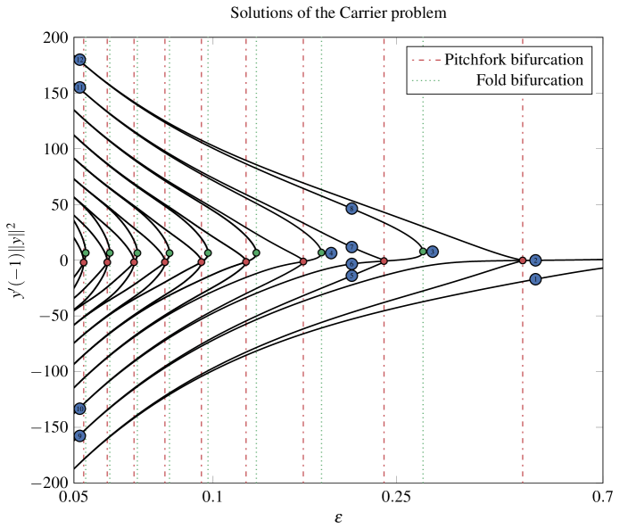
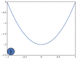
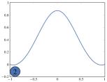
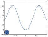
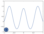
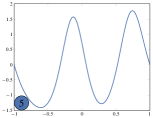
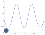
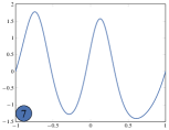
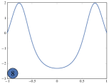
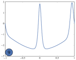
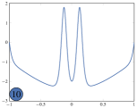
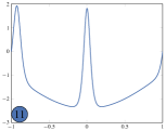
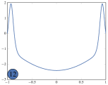
Fig. 2: Bifurcation diagram for Carrier’s equation (1) as a function of the singular perturbation parameter $\epsilon$. The diagram should be read from right to left, as $\epsilon\rightarrow 0$. For large $\epsilon$, there are two solutions; as $\epsilon\rightarrow 0$, the system undergoes alternating pitchfork and fold bifurcations (vertical lines). Green circles denote fold bifurcations; red circles denote pitchfork bifurcations; blue circles refer to solutions shown in the panels.

The central task of bifurcation theory is to determine how the number of solutions to an equation changes as a parameter is varied. The main algorithm used to compute this is the combination of arclength continuation and branch switching, as invented by Keller in 1977 [11] and implemented in popular software packages such as AUTO [7]. This algorithm is mature and highly successful, but has a significant drawback: it can only compute that part of the bifurcation diagram connected to the initial data, i.e. it computes connected components of the bifurcation diagram and cannot “jump” from one disconnected component to another. Unfortunately, the bifurcation diagram for Carrier’s problem is indeed disconnected: from any initial datum branch switching discovers at most four solutions, as we will see shortly. Since we already know from the analysis of Section 1 that at least eight solutions exist for moderate values of $\epsilon$, branch switching along $\epsilon\to 0$ offers only a limited insight into the solutions of (1).

In recent work, Farrell, Beentjes & Birkisson have developed an entirely new algorithm for computing bifurcation diagrams, called deflated continuation [9]. One of the central advantages of deflated continuation is that it is capable of computing disconnected bifurcation diagrams, such as that arising in Carrier’s problem. The main weakness of branch switching is that it relies on identifying critical points at which different branches meet; this is what renders it incapable of discovering branches that do not meet the known data at any point. In contrast, deflated continuation relies instead on a deflation technique for eliminating known solutions from consideration. Suppose $N$ regular solutions $y_{1},y_{2},\dots,y_{N}$ are known to a discretization of (1). Deflation constructs a new problem residual for Newton’s method with the property that no initial guess will converge to $y_{1},y_{2},\dots,y_{N}$. By guaranteeing that Newton’s method will not converge to known solutions, deflation enables the discovery of unknown branches, even if those branches are not connected to the known data. For more details, see Farrell et al. [9].

Equation (1) was discretized with $5\times 10^{4}$ standard piecewise linear finite elements using FEniCS [14] and PETSc [2]. We applied deflated continuation to this discretization from $\epsilon=\sqrt{1/2}$ to $\epsilon=1/20$, with a continuation step of $10^{-5}$ in $\epsilon^{2}$. Deflation was applied using the $H^{1}$ norm. All nonlinear systems were solved with Newton’s method and all arising linear systems were solved with LU factorization. Once deflated continuation had completed, arclength continuation was applied backwards in $\epsilon$ from the solutions found at $\epsilon=1/20$. The intricate bifurcation diagram computed in this way is shown in Figure 2.

The algorithm discovers two solutions to (1) for $\epsilon=\sqrt{1/2}$ from the initial guess ${y}(x)=1$; at $\epsilon=1/20$, 36 solutions were found. The system undergoes an initial pitchfork bifurcation at $\epsilon\approx 0.4689$, and subsequently alternates between fold and pitchfork bifurcations. At each bifurcation, two new solutions come into existence, and thus there are regions of the diagram for which the claim of Bender & Orszag that the number of solutions is divisible by 4 does not hold. These regions are precisely the gaps between each fold bifurcation and its subsequent pitchfork. However, these gaps tend to zero as $\epsilon\rightarrow 0$.

The diagram is highly fragmented; no connected component comprises more than four solutions, which is why branch switching applied to this problem can never discover more than four solutions from any single initial datum. We observe that each connected component is characterized by the number of interior maxima $M$. The lowest component comprises a single branch that undergoes no bifurcations, and corresponds to $M=0$; this branch exists for all $\epsilon$ and is shown in panel 1 of Figure 2. The next component ($M=1$) also exists for all $\epsilon$, and is shown in panel 2 of Figure 2. After the pitchfork bifurcation it comprises three solutions, one with an interior spike but no boundary spikes, one with no interior spike but a boundary spike on the left (as in Figure 1(b)), and one with no interior spike but a boundary spike on the right (as in Figure 1(c)).

The other components do not exist for large $\epsilon$, and come into existence at fold bifurcations as $\epsilon$ is reduced (panels 3 and 4 of Figure 2). Between each fold and its subsequent pitchfork bifurcation, the two solutions are symmetric with $n$ local maxima; both begin with $y^{\prime}(-1)>0$. In one of these solutions the maxima are more concentrated near $x=0$, whereas in the other there are maxima near $x=\pm 1$. This is illustrated in Figure 3 for $M=2$ and Figure 5 for $M=3$. The symmetry-breaking pitchfork bifurcation occurs on the branch where the maxima are concentrated near $x=0$ close to (but not exactly at) the value of $\epsilon$ for which $y^{\prime}(\pm 1)=0$. The new branches consist of solutions where one maximum leaves the centre and approaches one of the boundaries. This is illustrated in the middle row of panels of Figure 2 for $M=2$ and Figure 5 for $M=3$. As $\epsilon\rightarrow 0$, the symmetric solution with maxima concentrated near the centre tends to a solution with $M$ interior spikes; the symmetric solution with maxima near $x=\pm 1$ tends to a solution with 2 boundary layer spikes and $M-2$ interior spikes; the solutions emanating from the pitchfork bifurcation tend to solutions with 1 boundary layer spike and $M-1$ interior spikes. This is illustrated in the bottom row of panels of Figure 2 for $M=2$ and Figure 6 for $M=3$.

There are two further remarks to make regarding these observations. The first is that the number of interior maxima $M$ does not change through the bifurcations; hence our observation that each disconnected component is characterized by $M$. One consequence of this is that the four solutions we can generate by choosing different combinations of boundary layers (4) for a given number of interior spikes are not all on the same component of the bifurcation diagram. For example, in Figure 1, solutions (b) and (c) are connected in the bifurcation diagram, but lie on a different component to solutions (a) and (d), which are themselves on different components.

The second is that close to the bifurcations the oscillations fill the domain. Thus a boundary layer analysis in which there are a finite number of interior spikes separated from boundary layers by a spike-free outer region will never be able to capture the bifurcations. To capture the bifurcations we need to generate asymptotic solutions in which the interior spikes go all the way to the boundary.

Deflated continuation has successfully revealed an enormous amount of information regarding the solutions to (1), but it does not explain why the bifurcation diagram possesses this structure or predict the locations of the alternating fold and pitchfork bifurcations. Using the intuition we have gained from the numerical results, we now turn to asymptotic methods to see if we can predict these features analytically.

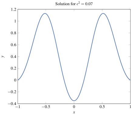
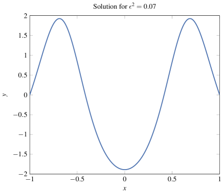
Fig. 3: The two solutions for $M=2$ at $\epsilon^{2}=0.07$, between the first fold (at $\epsilon^{2}\approx 0.08135$) and its subsequent pitchfork (at $\epsilon^{2}\approx 0.05509$). The maxima in (a) are more concentrated towards the centre, whereas (b) has maxima near the boundaries.

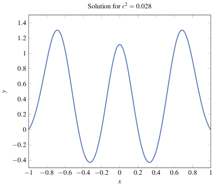
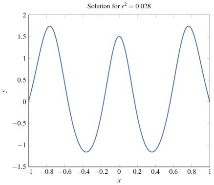
Fig. 4: The two solutions for $M=3$ at $\epsilon^{2}=0.028$, between its originating fold (at $\epsilon^{2}\approx 0.02953$) and its subsequent pitchfork (at $\epsilon^{2}\approx 0.02466$). The maxima in (a) are more concentrated towards the centre, whereas (b) has maxima near the boundaries. Compare to Figure 3, the corresponding diagram for $M=2$.

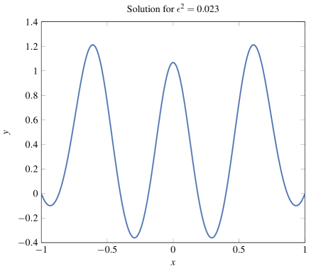
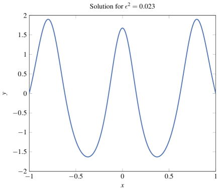
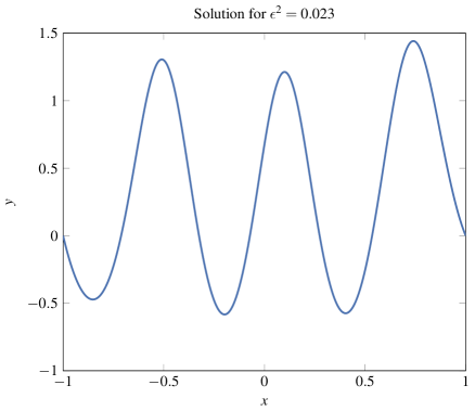
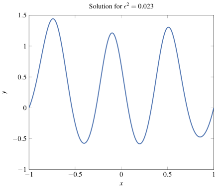
Fig. 5: The four solutions for $M=3$ at $\epsilon^{2}=0.023$, after its pitchfork bifurcation at $\epsilon^{2}\approx 0.02466$. The two symmetric solutions (a) and (b) lie on the same branch as 5a and 5b respectively. The branches (c) and (d) have bifurcated from (a) and are characterized by one of the interior maxima approaching the boundary. Compare to the middle row of panels of Figure 2, the corresponding solutions for $M=2$.

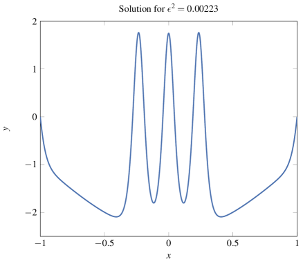
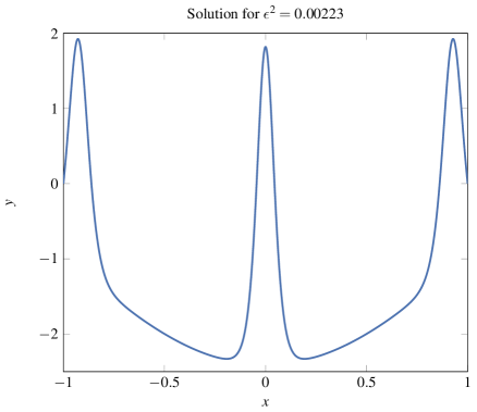
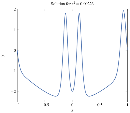
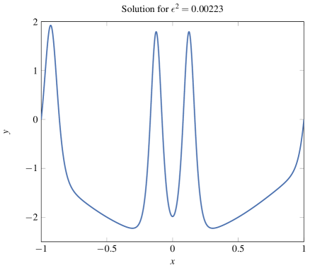
Fig. 6: The four solutions for $M=3$ at $\epsilon^{2}=0.00223$. The solutions are labeled as in 5. The symmetric solution with maxima near the centre has $M$ interior layers; the symmetric solution with maxima near the boundary has 2 boundary layers and $M-2$ interior layers; the asymmetric branches have 1 boundary layer and $M-1$ interior layers. Compare to the bottom row of panels of Figure 2, the corresponding diagram for $M=2$.

3 Asymptotic analysis

3.1 Asymptotic approximation using Kuzmak’s method

To be able to predict the bifurcations we have seen in solutions of (1) we need to be able to generate asymptotic solutions in which the interior spikes fill the domain, that is, solutions which are rapidly oscillating. We construct such asymptotic solutions using the method of Kuzmak [12].

We need to allow the frequency of the oscillation to vary slowly. Thus (as in the WKB method) we define the fast scale as $X=\phi(x)/\epsilon$, where the function $\phi(x)$ is to be determined. We then look for solutions $y(x,X)$, treating the slow scale $x$ and the fast scale $X$ as independent. We remove the indeterminacy this generates, and avoid secular terms in $X$, by imposing exact periodicity in $X$ with period 1.

From the chain rule we have

$$\mathchoice{\frac{\mathrm{d}y}{\mathrm{d}x}}{\mathrm{d}y/\mathrm{d}x}{\mathrm{d}y/\mathrm{d}x}{\mathrm{d}y/\mathrm{d}x} = y_{x}+\frac{\phi^{\prime}}{\epsilon}y_{X},$$

$$\mathchoice{\frac{\mathrm{d}^{2}y}{\mathrm{d}x^{2}}}{\mathrm{d}^{2}y/\mathrm{d}x^{2}}{\mathrm{d}^{2}y/\mathrm{d}x^{2}}{\mathrm{d}^{2}y/\mathrm{d}x^{2}} = y_{xx}+\frac{2\phi^{\prime}}{\epsilon}y_{xX}+\frac{\phi^{\prime\prime}}{\epsilon}y_{X}+\frac{(\phi^{\prime})^{2}}{\epsilon^{2}}y_{XX},$$

where $\phi^{\prime}=\mathchoice{\frac{\mathrm{d}\phi}{\mathrm{d}x}}{\mathrm{d}\phi/\mathrm{d}x}{\mathrm{d}\phi/\mathrm{d}x}{\mathrm{d}\phi/\mathrm{d}x}$, and a subscript denotes partial differentiation. Thus equation (1) becomes

$$(\phi^{\prime})^{2}y_{XX}+\epsilon(2\phi^{\prime}y_{xX}+\phi^{\prime\prime}y_{X})+\epsilon^{2}y_{xx}+2(1-x^{2})y+y^{2}=1.$$ (7)

We now pose a series expansion in powers of $\epsilon$:

$$y\sim y_{0}+\epsilon y_{1}+\cdots.$$

At leading order this gives

$$(\phi^{\prime})^{2}\mathchoice{\frac{\partial^{2}y_{0}}{{\partial}X^{2}}}{\partial^{2}y_{0}/{\partial}X^{2}}{\partial^{2}y_{0}/{\partial}X^{2}}{\partial^{2}y_{0}/{\partial}X^{2}}+2(1-x^{2})y_{0}+y_{0}^{2}=1,$$ (8)

with $y_{0}$ periodic in $X$, with period 1. If (8) were a linear equation then the solutions would be exponentials and our asymptotic method would simply be the WKB method. The fact that (8) is nonlinear means the fast oscillator is not simply harmonic, and we have to work a little bit harder to describe the oscillations.

Multiplying (8) by $2\mathchoice{\frac{{\partial}y_{0}}{{\partial}X}}{{\partial}y_{0}/{\partial}X}{{\partial}y_{0}/{\partial}X}{{\partial}y_{0}/{\partial}X}$ and integrating gives

$$(\phi^{\prime})^{2}\left(\mathchoice{\frac{{\partial}y_{0}}{{\partial}X}}{{\partial}y_{0}/{\partial}X}{{\partial}y_{0}/{\partial}X}{{\partial}y_{0}/{\partial}X}\right)^{2}+2(1-x^{2})y_{0}^{2}+\frac{2}{3}y_{0}^{3}=2y_{0}+A(x),$$

where the constant of integration, $A$, depends on the slow scale $x$. Separating the variables and integrating again gives

$$\pm\phi^{\prime}\int_{0}^{y_{0}}\frac{\mathrm{d}y}{(A(x)+2y-2(1-x^{2})y^{2}-2y^{3}/3)^{1/2}}=X+\mu(x).$$ (9)

The relevant values of $A(x)$ are those for which the cubic in the denominator has three real roots, $Y_{0}<Y_{1}<Y_{2}$, say. The cubic is positive for values $Y_{1}<y<Y_{2}$. Periodicity of $y_{0}$ in $X$ is achieved by integrating the positive square root from $Y_{1}$ to $Y_{2}$ and then the negative square root from $Y_{2}$ to $Y_{1}$. Setting the period equal to unity therefore implies

$$\phi^{\prime}=\left(2\int_{Y_{1}}^{Y_{2}}\frac{\mathrm{d}y}{(A(x)+2y-2(1-x^{2})y^{2}-2y^{3}/3)^{1/2}}\right)^{-1}.$$ (10)

Note that $\phi^{\prime}$ depends on $A$ but not on $\mu$.

We have thus far determined the leading-order solution $y_{0}$ and the fast scale of oscillation $\phi$ in terms of the two unknown slow functions $A(x)$ and $\mu(x)$, which correspond roughly to the slowly modulated amplitude and phase of the oscillation. To determine these functions we need to proceed to higher orders in the asymptotic expansion.

Equating coefficients of $\epsilon$ in (7) gives

$$(\phi^{\prime})^{2}\mathchoice{\frac{\partial^{2}y_{1}}{{\partial}X^{2}}}{\partial^{2}y_{1}/{\partial}X^{2}}{\partial^{2}y_{1}/{\partial}X^{2}}{\partial^{2}y_{1}/{\partial}X^{2}}+2(1-x^{2})y_{1}+2y_{0}y_{1}=-2\phi^{\prime}\mathchoice{\frac{\partial^{2}y_{0}}{{\partial}x{\partial}X}}{\partial^{2}y_{0}/{\partial}x{\partial}X}{\partial^{2}y_{0}/{\partial}x{\partial}X}{\partial^{2}y_{0}/{\partial}x{\partial}X}-\phi^{\prime\prime}\mathchoice{\frac{{\partial}y_{0}}{{\partial}X}}{{\partial}y_{0}/{\partial}X}{{\partial}y_{0}/{\partial}X}{{\partial}y_{0}/{\partial}X}.$$

The homogeneous version of this equation is satisfied by both

$$\mathchoice{\frac{{\partial}y_{0}}{{\partial}A}}{{\partial}y_{0}/{\partial}A}{{\partial}y_{0}/{\partial}A}{{\partial}y_{0}/{\partial}A}\quad\mbox{ and }\quad\mathchoice{\frac{{\partial}y_{0}}{{\partial}\mu}}{{\partial}y_{0}/{\partial}\mu}{{\partial}y_{0}/{\partial}\mu}{{\partial}y_{0}/{\partial}\mu}.$$

Thus, by the Fredholm alternative, in order for there to be a solution for $y_{1}$ we have the solvability conditions

$$2\phi^{\prime}\int_{0}^{1}\mathchoice{\frac{\partial^{2}y_{0}}{{\partial}x{\partial}X}}{\partial^{2}y_{0}/{\partial}x{\partial}X}{\partial^{2}y_{0}/{\partial}x{\partial}X}{\partial^{2}y_{0}/{\partial}x{\partial}X}\mathchoice{\frac{{\partial}y_{0}}{{\partial}A}}{{\partial}y_{0}/{\partial}A}{{\partial}y_{0}/{\partial}A}{{\partial}y_{0}/{\partial}A}\,\mathrm{d}X+\phi^{\prime\prime}\int_{0}^{1}\mathchoice{\frac{{\partial}y_{0}}{{\partial}X}}{{\partial}y_{0}/{\partial}X}{{\partial}y_{0}/{\partial}X}{{\partial}y_{0}/{\partial}X}\mathchoice{\frac{{\partial}y_{0}}{{\partial}A}}{{\partial}y_{0}/{\partial}A}{{\partial}y_{0}/{\partial}A}{{\partial}y_{0}/{\partial}A}\,\mathrm{d}X = 0,$$ (11)

$$2\phi^{\prime}\int_{0}^{1}\mathchoice{\frac{\partial^{2}y_{0}}{{\partial}x{\partial}X}}{\partial^{2}y_{0}/{\partial}x{\partial}X}{\partial^{2}y_{0}/{\partial}x{\partial}X}{\partial^{2}y_{0}/{\partial}x{\partial}X}\mathchoice{\frac{{\partial}y_{0}}{{\partial}\mu}}{{\partial}y_{0}/{\partial}\mu}{{\partial}y_{0}/{\partial}\mu}{{\partial}y_{0}/{\partial}\mu}\,\mathrm{d}X+\phi^{\prime\prime}\int_{0}^{1}\mathchoice{\frac{{\partial}y_{0}}{{\partial}X}}{{\partial}y_{0}/{\partial}X}{{\partial}y_{0}/{\partial}X}{{\partial}y_{0}/{\partial}X}\mathchoice{\frac{{\partial}y_{0}}{{\partial}\mu}}{{\partial}y_{0}/{\partial}\mu}{{\partial}y_{0}/{\partial}\mu}{{\partial}y_{0}/{\partial}\mu}\,\mathrm{d}X = 0.$$ (12)

These equations are our differential equations for $A$ and $\mu$ as functions of $x$.

To enable us to write down these differential equations explicitly, let us define the function $Y(X,x,\Phi,A)$ by

$$\Phi\int_{Y_{1}(A,x)}^{Y}\frac{\mathrm{d}y}{c(A,x,y)^{1/2}} = X,\quad 0<X<X^{*}(A,x,\Phi)$$ (13)

$$X^{*}(A,x,\Phi)+\Phi\int^{Y_{2}(A,x)}_{Y}\frac{\mathrm{d}y}{c(A,x,y)^{1/2}} = X,\quad X^{*}(A,x,\Phi)<X<2X^{*}(A,x,\Phi),\qquad$$ (14)

and the function $\Phi(A,x)$ by

$$\Phi(A,x)=\left(2\int_{Y_{1}(A,x)}^{Y_{2}(A,x)}\frac{\mathrm{d}y}{c(A,x,y)^{1/2}}\right)^{-1},$$ (15)

where

$$c(A,x,y) = A+2y-2(1-x^{2})y^{2}-\frac{2}{3}y^{3},$$ (16)

$$X^{*}(A,x,\Phi) = \Phi\int_{Y_{1}(A,x)}^{Y_{2}(A,x)}\frac{\mathrm{d}y}{c(A,x,y)^{1/2}}.$$ (17)

Then $y_{0}=Y(X+\mu(x),x,\Phi(A(x),x),A(x))$. Note that (15) gives $X^{*}(A,x,\Phi(x,A))=1/2$ as we would expect, since $\Phi(A(x),x)=\phi^{\prime}$ was chosen to make the period 1 in $X$. We now have

$$\mathchoice{\frac{\partial^{2}y_{0}}{{\partial}x{\partial}X}}{\partial^{2}y_{0}/{\partial}x{\partial}X}{\partial^{2}y_{0}/{\partial}x{\partial}X}{\partial^{2}y_{0}/{\partial}x{\partial}X} = \mathchoice{\frac{\partial^{2}Y}{{\partial}x{\partial}X}}{\partial^{2}Y/{\partial}x{\partial}X}{\partial^{2}Y/{\partial}x{\partial}X}{\partial^{2}Y/{\partial}x{\partial}X}+\mathchoice{\frac{\partial^{2}Y}{{\partial}\Phi{\partial}X}}{\partial^{2}Y/{\partial}\Phi{\partial}X}{\partial^{2}Y/{\partial}\Phi{\partial}X}{\partial^{2}Y/{\partial}\Phi{\partial}X}\left(\mathchoice{\frac{{\partial}\Phi}{{\partial}x}}{{\partial}\Phi/{\partial}x}{{\partial}\Phi/{\partial}x}{{\partial}\Phi/{\partial}x}+A^{\prime}\mathchoice{\frac{{\partial}\Phi}{{\partial}A}}{{\partial}\Phi/{\partial}A}{{\partial}\Phi/{\partial}A}{{\partial}\Phi/{\partial}A}\right)+\mathchoice{\frac{\partial^{2}Y}{{\partial}A{\partial}X}}{\partial^{2}Y/{\partial}A{\partial}X}{\partial^{2}Y/{\partial}A{\partial}X}{\partial^{2}Y/{\partial}A{\partial}X}A^{\prime}+\mathchoice{\frac{\partial^{2}Y}{{\partial}X^{2}}}{\partial^{2}Y/{\partial}X^{2}}{\partial^{2}Y/{\partial}X^{2}}{\partial^{2}Y/{\partial}X^{2}}\mu^{\prime},$$

$$\mathchoice{\frac{{\partial}y_{0}}{{\partial}A}}{{\partial}y_{0}/{\partial}A}{{\partial}y_{0}/{\partial}A}{{\partial}y_{0}/{\partial}A} = \mathchoice{\frac{{\partial}Y}{{\partial}A}}{{\partial}Y/{\partial}A}{{\partial}Y/{\partial}A}{{\partial}Y/{\partial}A}+\mathchoice{\frac{{\partial}Y}{{\partial}\Phi}}{{\partial}Y/{\partial}\Phi}{{\partial}Y/{\partial}\Phi}{{\partial}Y/{\partial}\Phi}\mathchoice{\frac{{\partial}\Phi}{{\partial}A}}{{\partial}\Phi/{\partial}A}{{\partial}\Phi/{\partial}A}{{\partial}\Phi/{\partial}A},$$

$$\mathchoice{\frac{{\partial}y_{0}}{{\partial}\mu}}{{\partial}y_{0}/{\partial}\mu}{{\partial}y_{0}/{\partial}\mu}{{\partial}y_{0}/{\partial}\mu} = \mathchoice{\frac{{\partial}Y}{{\partial}X}}{{\partial}Y/{\partial}X}{{\partial}Y/{\partial}X}{{\partial}Y/{\partial}X},$$

$$\phi^{\prime\prime} = \mathchoice{\frac{{\partial}\Phi}{{\partial}x}}{{\partial}\Phi/{\partial}x}{{\partial}\Phi/{\partial}x}{{\partial}\Phi/{\partial}x}+A^{\prime}\mathchoice{\frac{{\partial}\Phi}{{\partial}A}}{{\partial}\Phi/{\partial}A}{{\partial}\Phi/{\partial}A}{{\partial}\Phi/{\partial}A},$$

and the solvability conditions are

$$2\Phi\int_{0}^{1}\left(\mathchoice{\frac{\partial^{2}Y}{{\partial}x{\partial}X}}{\partial^{2}Y/{\partial}x{\partial}X}{\partial^{2}Y/{\partial}x{\partial}X}{\partial^{2}Y/{\partial}x{\partial}X}+\mathchoice{\frac{\partial^{2}Y}{{\partial}\Phi{\partial}X}}{\partial^{2}Y/{\partial}\Phi{\partial}X}{\partial^{2}Y/{\partial}\Phi{\partial}X}{\partial^{2}Y/{\partial}\Phi{\partial}X}\left(\mathchoice{\frac{{\partial}\Phi}{{\partial}x}}{{\partial}\Phi/{\partial}x}{{\partial}\Phi/{\partial}x}{{\partial}\Phi/{\partial}x}+A^{\prime}\mathchoice{\frac{{\partial}\Phi}{{\partial}A}}{{\partial}\Phi/{\partial}A}{{\partial}\Phi/{\partial}A}{{\partial}\Phi/{\partial}A}\right)+\mathchoice{\frac{\partial^{2}Y}{{\partial}A{\partial}X}}{\partial^{2}Y/{\partial}A{\partial}X}{\partial^{2}Y/{\partial}A{\partial}X}{\partial^{2}Y/{\partial}A{\partial}X}A^{\prime}+\mathchoice{\frac{\partial^{2}Y}{{\partial}X^{2}}}{\partial^{2}Y/{\partial}X^{2}}{\partial^{2}Y/{\partial}X^{2}}{\partial^{2}Y/{\partial}X^{2}}\mu^{\prime}\right)\left(\mathchoice{\frac{{\partial}Y}{{\partial}A}}{{\partial}Y/{\partial}A}{{\partial}Y/{\partial}A}{{\partial}Y/{\partial}A}+\mathchoice{\frac{{\partial}Y}{{\partial}\Phi}}{{\partial}Y/{\partial}\Phi}{{\partial}Y/{\partial}\Phi}{{\partial}Y/{\partial}\Phi}\mathchoice{\frac{{\partial}\Phi}{{\partial}A}}{{\partial}\Phi/{\partial}A}{{\partial}\Phi/{\partial}A}{{\partial}\Phi/{\partial}A}\right)\,\mathrm{d}X$$

$$\mbox{ }+\left(\mathchoice{\frac{{\partial}\Phi}{{\partial}x}}{{\partial}\Phi/{\partial}x}{{\partial}\Phi/{\partial}x}{{\partial}\Phi/{\partial}x}+A^{\prime}\mathchoice{\frac{{\partial}\Phi}{{\partial}A}}{{\partial}\Phi/{\partial}A}{{\partial}\Phi/{\partial}A}{{\partial}\Phi/{\partial}A}\right)\int_{0}^{1}\mathchoice{\frac{{\partial}Y}{{\partial}X}}{{\partial}Y/{\partial}X}{{\partial}Y/{\partial}X}{{\partial}Y/{\partial}X}\left(\mathchoice{\frac{{\partial}Y}{{\partial}A}}{{\partial}Y/{\partial}A}{{\partial}Y/{\partial}A}{{\partial}Y/{\partial}A}+\mathchoice{\frac{{\partial}Y}{{\partial}\Phi}}{{\partial}Y/{\partial}\Phi}{{\partial}Y/{\partial}\Phi}{{\partial}Y/{\partial}\Phi}\mathchoice{\frac{{\partial}\Phi}{{\partial}A}}{{\partial}\Phi/{\partial}A}{{\partial}\Phi/{\partial}A}{{\partial}\Phi/{\partial}A}\right)\,\mathrm{d}X = 0,\hskip 56.9055pt$$ (18)

$$2\Phi\int_{0}^{1}\left(\mathchoice{\frac{\partial^{2}Y}{{\partial}x{\partial}X}}{\partial^{2}Y/{\partial}x{\partial}X}{\partial^{2}Y/{\partial}x{\partial}X}{\partial^{2}Y/{\partial}x{\partial}X}+\mathchoice{\frac{\partial^{2}Y}{{\partial}\Phi{\partial}X}}{\partial^{2}Y/{\partial}\Phi{\partial}X}{\partial^{2}Y/{\partial}\Phi{\partial}X}{\partial^{2}Y/{\partial}\Phi{\partial}X}\left(\mathchoice{\frac{{\partial}\Phi}{{\partial}x}}{{\partial}\Phi/{\partial}x}{{\partial}\Phi/{\partial}x}{{\partial}\Phi/{\partial}x}+A^{\prime}\mathchoice{\frac{{\partial}\Phi}{{\partial}A}}{{\partial}\Phi/{\partial}A}{{\partial}\Phi/{\partial}A}{{\partial}\Phi/{\partial}A}\right)+\mathchoice{\frac{\partial^{2}Y}{{\partial}A{\partial}X}}{\partial^{2}Y/{\partial}A{\partial}X}{\partial^{2}Y/{\partial}A{\partial}X}{\partial^{2}Y/{\partial}A{\partial}X}A^{\prime}+\mathchoice{\frac{\partial^{2}Y}{{\partial}X^{2}}}{\partial^{2}Y/{\partial}X^{2}}{\partial^{2}Y/{\partial}X^{2}}{\partial^{2}Y/{\partial}X^{2}}\mu^{\prime}\right)\mathchoice{\frac{{\partial}Y}{{\partial}X}}{{\partial}Y/{\partial}X}{{\partial}Y/{\partial}X}{{\partial}Y/{\partial}X}\,\mathrm{d}X$$

$$\mbox{ }+\left(\mathchoice{\frac{{\partial}\Phi}{{\partial}x}}{{\partial}\Phi/{\partial}x}{{\partial}\Phi/{\partial}x}{{\partial}\Phi/{\partial}x}+A^{\prime}\mathchoice{\frac{{\partial}\Phi}{{\partial}A}}{{\partial}\Phi/{\partial}A}{{\partial}\Phi/{\partial}A}{{\partial}\Phi/{\partial}A}\right)\int_{0}^{1}\left(\mathchoice{\frac{{\partial}Y}{{\partial}X}}{{\partial}Y/{\partial}X}{{\partial}Y/{\partial}X}{{\partial}Y/{\partial}X}\right)^{2}\,\mathrm{d}X = 0.\hskip 56.9055pt$$ (19)

Because of periodicity, any terms which are exact derivatives in $X$ will integrate to zero. Moreover, $Y$ and its derivatives with respect to $x$, $\Phi$ and $A$ are even, while $Y_{X}$ and derivatives with respect to $x$, $\Phi$ and $A$ are odd. Thus in fact equation (18) reduces to

$$\mu^{\prime}=0,$$ (20)

so that $\mu$ is in fact constant. Since $Y$ is periodic in $X$ with period $1$ we may take $\mu\in[0,1)$ without loss of generality. Equation (19) can be written as

$$\Phi\mathchoice{\frac{{\partial}\overline{Y_{X}^{2}}}{{\partial}x}}{{\partial}\overline{Y_{X}^{2}}/{\partial}x}{{\partial}\overline{Y_{X}^{2}}/{\partial}x}{{\partial}\overline{Y_{X}^{2}}/{\partial}x}+\Phi\left(\mathchoice{\frac{{\partial}\Phi}{{\partial}x}}{{\partial}\Phi/{\partial}x}{{\partial}\Phi/{\partial}x}{{\partial}\Phi/{\partial}x}+A^{\prime}\mathchoice{\frac{{\partial}\Phi}{{\partial}A}}{{\partial}\Phi/{\partial}A}{{\partial}\Phi/{\partial}A}{{\partial}\Phi/{\partial}A}\right)\mathchoice{\frac{{\partial}\overline{Y_{X}^{2}}}{{\partial}\Phi}}{{\partial}\overline{Y_{X}^{2}}/{\partial}\Phi}{{\partial}\overline{Y_{X}^{2}}/{\partial}\Phi}{{\partial}\overline{Y_{X}^{2}}/{\partial}\Phi}+\Phi A^{\prime}\mathchoice{\frac{{\partial}\overline{Y_{X}^{2}}}{{\partial}A}}{{\partial}\overline{Y_{X}^{2}}/{\partial}A}{{\partial}\overline{Y_{X}^{2}}/{\partial}A}{{\partial}\overline{Y_{X}^{2}}/{\partial}A}+\left(\mathchoice{\frac{{\partial}\Phi}{{\partial}x}}{{\partial}\Phi/{\partial}x}{{\partial}\Phi/{\partial}x}{{\partial}\Phi/{\partial}x}+A^{\prime}\mathchoice{\frac{{\partial}\Phi}{{\partial}A}}{{\partial}\Phi/{\partial}A}{{\partial}\Phi/{\partial}A}{{\partial}\Phi/{\partial}A}\right)\overline{Y_{X}^{2}} = 0,$$ (21)

where

$$\overline{Y_{X}^{2}}=\int_{0}^{1}\left(\mathchoice{\frac{{\partial}Y}{{\partial}X}}{{\partial}Y/{\partial}X}{{\partial}Y/{\partial}X}{{\partial}Y/{\partial}X}\right)^{2}\,\mathrm{d}X.$$

Remarkably, eqn (21) is simply

$$\Phi\mathchoice{\frac{\mathrm{d}\overline{Y_{X}^{2}}}{\mathrm{d}x}}{\mathrm{d}\overline{Y_{X}^{2}}/\mathrm{d}x}{\mathrm{d}\overline{Y_{X}^{2}}/\mathrm{d}x}{\mathrm{d}\overline{Y_{X}^{2}}/\mathrm{d}x}+\mathchoice{\frac{\mathrm{d}\Phi}{\mathrm{d}x}}{\mathrm{d}\Phi/\mathrm{d}x}{\mathrm{d}\Phi/\mathrm{d}x}{\mathrm{d}\Phi/\mathrm{d}x}\overline{Y_{X}^{2}}=\mathchoice{\frac{\mathrm{d}}{\mathrm{d}x}}{\mathrm{d}/\mathrm{d}x}{\mathrm{d}/\mathrm{d}x}{\mathrm{d}/\mathrm{d}x}\left(\Phi\overline{Y_{X}^{2}}\right)=0,$$ (22)

so that

$$\Phi\overline{Y_{X}^{2}}=\mbox{constant}=k,$$ (23)

say. Now, since

$$\Phi^{2}\left(\mathchoice{\frac{{\partial}Y}{{\partial}X}}{{\partial}Y/{\partial}X}{{\partial}Y/{\partial}X}{{\partial}Y/{\partial}X}\right)^{2}=A+2Y-2(1-x^{2})Y^{2}-\frac{2}{3}Y^{3},$$

$$\Phi\overline{Y_{X}^{2}} = \frac{1}{\Phi}\int_{0}^{1}\left(A+2Y-2(1-x^{2})Y^{2}-\frac{2}{3}Y^{3}\right)\,\mathrm{d}X$$ (24)

$$= 2\int_{Y_{1}(A,x)}^{Y_{2}(A,x)}\left(A+2y-2(1-x^{2})y^{2}-\frac{2}{3}y^{3}\right)^{1/2}\,\mathrm{d}y=k.$$

This is an implicit solution for $A(x)$, and is equivalent to equation (54) in [17], which was determined by other means. In fact, it is nothing more than the principle of adiabatic invariance [13], which states that a trajectory can be approximated by moving slowly from one closed orbit to another as $x$ varies (closed in terms of the fast scale $X$ when treating $x$ as constant) in such a way that the enclosed area remains constant. We see that equation (22) follows directly from (12) once we realise that $\mathchoice{\frac{{\partial}y_{0}}{{\partial}\mu}}{{\partial}y_{0}/{\partial}\mu}{{\partial}y_{0}/{\partial}\mu}{{\partial}y_{0}/{\partial}\mu}=\mathchoice{\frac{{\partial}y_{0}}{{\partial}X}}{{\partial}y_{0}/{\partial}X}{{\partial}y_{0}/{\partial}X}{{\partial}y_{0}/{\partial}X}$.

In Fig. 7 we show $A$ as a function of $x$ for integer values of $k$ between $1$ and $15$. For $0<k<k_{1}\approx 6.78823$ the solution (24) is valid in the whole domain $-1<x<1$. However, we will see in §3.2 that for $k>k_{1}$ there are turning points at $x=\pm x^{*}$ at which $\Phi=0$. For $|x|>x^{*}$ the solution will cease to be oscillatory and will instead be described by the outer solution (2). Thus values $0<k<k_{1}$ correspond to solutions in which the spikes fill the domain, while values $k>k_{1}$ correspond to solutions in which there is an interior region near $x=0$ containing spikes, separated from the boundary layers by the spike-less outer solution.

In Fig. 8 we show $Y$ as a function of $X$ when $k=5$ and $A$ is given by (24), for $x=0$, $0.2$, $0.4$, $0.6$, $0.8$, $1$. This illustrates the fact that the form of the oscillation varies with position, which is due to the leading-order nonlinearity in (1), which causes the underlying oscillator (8) to be nonlinear.

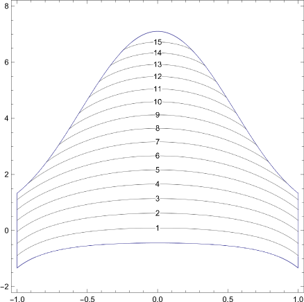
Fig. 7: $A$ as a function of $x$ for different values of $k$. The upper and lower curves are $A_{1}(x)$ and $A_{2}(x)$ respectively. For $0<k<k_{1}\approx 6.78823$ the solution $A(x)$ stays between $A_{1}$ and $A_{2}$ for all $-1<x<1$. For $k>k_{1}$ there are turning points at $x=\pm x^{*}$ at which $A(\pm x^{*})=A_{1}(\pm x^{*})$.

Fig. 8: The function $Y(X,x,\Phi(x,A(x)),A(x)$ for $k=5$ at $x=0$ (bottom), $0.2$, $0.4$, $0.6$, $0.8$, and $1$ (top). Because of the leading-order nonlinearity in (1), the underlying oscillator (8) is nonlinear, so that the form of the oscillation (and not just the amplitude) varies with position.

We have now determined the leading-order solution, up to the imposition of the boundary conditions. To summarise, we have

$$y_{0}=Y\left(\frac{\phi(x)}{\epsilon}+\mu,x,\Phi(x,A(x)),A(x)\right),\qquad\phi^{\prime}(x)=\Phi(A(x),x),$$ (25)

where $Y(X,x,\Phi,A)$ is the function given by (13)-(14) and

$$\Phi = \left(2\int_{Y_{1}(A,x)}^{Y_{2}(A,x)}\frac{\mathrm{d}y}{(A+2y-2(1-x^{2})y^{2}-2y^{3}/3)^{1/2}}\right)^{-1},$$

$$k = 2\int_{Y_{1}(A,x)}^{Y_{2}(A,x)}\left(A+2y-2(1-x^{2})y^{2}-\frac{2}{3}y^{3}\right)^{1/2}\,\mathrm{d}y,$$

where $\mu$ and $k$ are constants to be determined by the boundary conditions. Note that we can choose $\phi(0)=0$ without loss of generality.

3.2 Turning Points

Before we investigate the imposition of the boundary conditions to determine the remaining unknown constants, we first discuss in more detail the turning points that may appear in the solution. These occur whenever $\phi^{\prime}(x)=0$, i.e. $\Phi(A(x),x)=0$. Looking at (15), we see this will happen when $Y_{0}\rightarrow Y_{1}$, that is, the left-most roots of $c(y)$ coalesce. (We might also expect something strange to happen when the right-most roots of $c(y)$ coalesce, that is, when $Y_{1}\rightarrow Y_{2}$. In that case, however, because the range of integration in (15) shrinks to zero at the same rate at which the integrand blows up, $\Phi$ remains finite. The case $Y_{1}\rightarrow Y_{2}$ corresponds to the limit in which the constant $k\rightarrow 0$.)

Thus, at the turning point, we have a double root of $c$, so that there is a simultaneous root of $c$ and $\mathchoice{\frac{{\partial}c}{{\partial}y}}{{\partial}c/{\partial}y}{{\partial}c/{\partial}y}{{\partial}c/{\partial}y}$. Such a double root occurs when $A=A_{1}(x)$ or $A=A_{2}(x)$ where

$$A_{1}(x) = \frac{2}{3}\left(5-9x^{2}+6x^{4}-2x^{6}+2(2-2x^{2}+x^{4})^{3/2}\right),$$

$$A_{2}(x) = \frac{2}{3}\left(5-9x^{2}+6x^{4}-2x^{6}-2(2-2x^{2}+x^{4})^{3/2}\right).$$

When $A(x)=A_{1}(x)$ the left most roots of $c(y)$ coalesce ($Y_{0}\rightarrow Y_{1}$). At $A(x)=A_{2}(x)$ the right most roots of $c(y)$ coalesce ($Y_{1}\rightarrow Y_{2}$). The functions $A_{1}(x)$ and $A_{2}(x)$ form the upper and lower boundaries in Fig. 7 respectively.

The limiting value of $k$ for which there are no turning points in $[-1,1]$ and the oscillations are present all the way to the boundary is given by $A(1)=A_{1}(1)$, that is, it is the value of $k$ for which the turning points lie at $x=\pm 1$. We find this is

$$k=k_{1}\approx 6.78823.$$

For $k>k_{1}$ there will be an interior region between the two turning points $x=\pm x^{*}$ in which the solution is rapidly oscillating (i.e. in which there are spikes), separated from the boundary layers by the spike-less outer solution (2).

3.3 Boundary conditions

Let us now seek to determine the remaining unknown constants $k$ and $\mu$ by imposing the boundary conditions on our asymptotic solution. We first look for solutions in which there are no turning points, that is, in which the Kuzmak approximation we have derived is valid all the way to the boundary. The conditions $y(-1)=y(1)=0$ imply

$$Y\left(\frac{\phi(\pm 1)}{\epsilon}+\mu,\pm 1,\Phi(\pm 1,A(\pm 1)),A(\pm 1)\right)=0.$$ (26)

Now, the function $Y(X,\pm 1,\Phi(\pm 1,A(\pm 1)),A(\pm 1))$ has two zeros in the unit cell $0<X<1$ (see Fig. 8). Let us denote the smaller by $X_{0}$; the larger is then given by $1-X_{0}$. Then, at leading order, (26) gives

$$\frac{\phi(1)}{\epsilon}+\mu=n\pm X_{0},\qquad\frac{\phi(-1)}{\epsilon}+\mu=m\pm X_{0},$$ (27)

where $n$, $m\in{\mathbb{Z}}$. These are two equations for the two unknown constants $k$ and $\mu$.

Eliminating $\phi(1)$, noting that $\phi(1)=-\phi(-1)$, gives the four possibilities

$$n+m=\quad 2\mu,\quad 2\mu,\quad-2X_{0}+2\mu,\quad 2X_{0}+2\mu,$$ (28)

corresponding to choosing the signs in (27) as $+-$, $-+$, $++$ and $--$ respectively. In the first two cases (which give a symmetric solution) we must have $\mu=0$ (corresponding to a solution with a minimum at the origin) or $\mu=1/2$ (corresponding to a solution with a maximum at the origin). We first analyse these symmetric solutions, and their associated bifurcations, before returning to consider the non-symmetric solutions.

3.4 Symmetric Solutions

We consider here solutions in which $\mu=0$ or $\mu=1/2$. In this case equations (27) reduce to

$$\frac{\phi(1)}{\epsilon}=n\pm X_{0}\qquad\mbox{ and }\qquad\frac{\phi(1)}{\epsilon}=n+\frac{1}{2}\pm X_{0},$$ (29)

respectively. We need to find the values of $k$ for which one of these equations is satisfied.

We show in Figure 9 the curves

$$n\pm X_{0}\quad\mbox{ (black)}\qquad\mbox{and}\qquad n+\frac{1}{2}\pm X_{0}\quad\mbox{ (blue)}$$

as a function of $k$ for $n$ in the range $20$ to $24$. The noses of these curves correspond to the value of $k$ at which $Y=Y_{X}=0$ at $x=\pm 1$, which means that $A(\pm 1)=0$. This corresponds to

$$k=k_{0}=\frac{16\times 3^{3/4}\pi^{3/2}}{5\Gamma(1/4)^{2}}\approx 3.08997.$$

Also shown in Figure 9 (green) are the curves $\phi(1)/\epsilon$ for $\epsilon=0.01+0.004j$ with $j$ ranging from $-2$ to $4$. For a given value of $\epsilon$, the intersections between the corresponding green curve and the black and blue curves give solutions of (29), and therefore correspond to symmetric solutions of (1). We see that as $\epsilon$ decreases there is a succession of fold bifurcations as a new pair of intersection points appears near $k=k_{0}$.

Initially, as $\epsilon$ decreases, one of the two new intersection points moves to the left and one to the right. However, the left-moving point soon reaches the nose of the blue/black curve, after which both intersection points move to the right, in the direction of increasing $k$. Eventually both approach the limiting value $k=k_{1}$, at which point a turning point appears near the boundary, and another analysis takes over, since the boundary conditions should not then be applied to the Kuzmak solution. After the turning point appears these solutions transition into solutions whose oscillations do not encompass the whole domain, but are restricted some smaller interval.

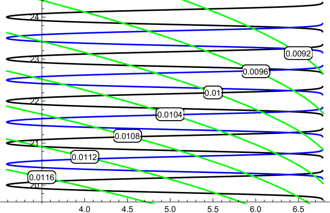
Fig. 9: The curves $n\pm X_{0}$ (black) and $n+1/2\pm X_{0}$ (blue) as a function of $k$ for $n$ in the range $20$ to $24$. Also shown are the curves $\phi(1)/\epsilon$ for values of $\epsilon$ indicated (green). The intersections between these curves give symmetric solutions of the problem.

In Figure 12 we show the figure analogous to Fig. 9 for $\epsilon=0.0335$. We illustrate the four intersection points, along with the corresponding asymptotic approximation of the solutions.

3.4.1 Maximum number of spikes

The number of maxima in each solution is the number of complete periods in $X$, which is

$$\frac{\phi(1)-\phi(-1)}{\epsilon}=\frac{2\phi(1)}{\epsilon}.$$

Since $\phi(1)$ is monotonically decreasing in $k$ (see Fig. 9), the largest value of $\phi(1)$ occurs for $k=k_{0}$. This gives

$$2\phi(1)\approx 0.472537.$$

Thus the maximum number of spikes is

$$\left\lfloor\frac{0.472537}{\epsilon}\right\rfloor$$

where $\lfloor x\rfloor$ denotes the largest integer less than $x$, in agreement with the results of [17].

3.4.2 Proportion of solutions with oscillations filling the domain

The description in the introduction indicated that we might gradually add spikes into the interior of the domain until there is no room to fit any more. Thus we might have expected that the proportion of solutions containing turning points (i.e. the proportion containing some spike-free region) should tend to 1 as $\epsilon\rightarrow 0$. However, minimum number of spikes which may be present in a solution which does not have turning points is given by the minimum value of

$$\left\lfloor\frac{2\phi(1)}{\epsilon}\right\rfloor$$

for $k_{0}<k<k_{1}$, which occurs when $k=k_{1}$, and is

$$\left\lfloor\frac{0.415}{\epsilon}\right\rfloor.$$

Only for solutions with fewer spikes will the oscillations not fill the domain. Thus the proportion of solutions which do not have turning points is approximately $0.12$ in the limit as $\epsilon\rightarrow 0$.

3.4.3 Position of the fold bifurcations

The fold bifurcation is not exactly at the nose of the blue or black curve in Fig. 9, though it approaches it as $\epsilon\rightarrow 0$. At the bifurcation point the green and blue/black curves are tangent, so that

$$\frac{1}{\epsilon}\mathchoice{\frac{\mathrm{d}\phi(1)}{\mathrm{d}k}}{\mathrm{d}\phi(1)/\mathrm{d}k}{\mathrm{d}\phi(1)/\mathrm{d}k}{\mathrm{d}\phi(1)/\mathrm{d}k}=-\mathchoice{\frac{\mathrm{d}X_{0}}{\mathrm{d}k}}{\mathrm{d}X_{0}/\mathrm{d}k}{\mathrm{d}X_{0}/\mathrm{d}k}{\mathrm{d}X_{0}/\mathrm{d}k},$$ (30)

which must be satisfied at the same time as

$$\frac{2\phi(1)}{\epsilon}=n-2X_{0}$$ (31)

(minus sign because the tangency is on the lower branch of the blue/black curve). Equations (30) and (31) form two equations for $k$ and $\epsilon$ as a function of $n$.

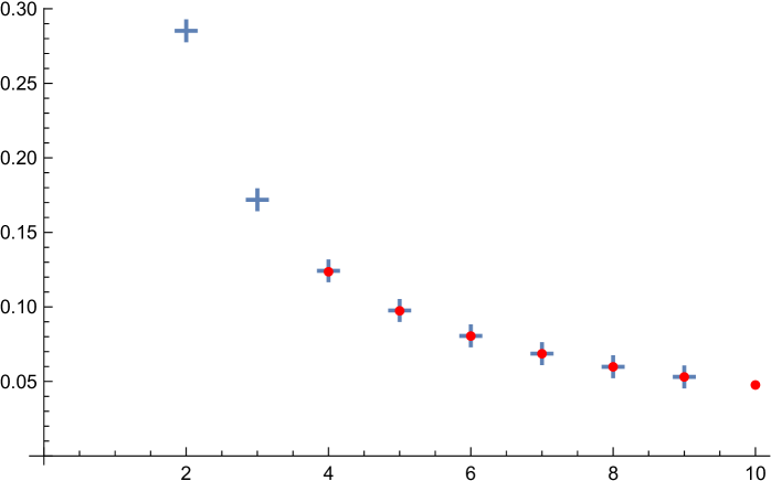
Fig. 10: The values of $\epsilon$ at the fold bifurcations, as a function of $n$. Equations (30) and (31) are valid in the limit $\epsilon\rightarrow 0$, corresponding to $n\rightarrow\infty$. The first value of $n$ for which a tangency point exists is $n=4$, which corresponds to the third fold bifurcation. Crosses indicate numerical results, circles the asymptotic approximation.

We can approximate (30), (31) in the limit of small $\epsilon$ (large $n$), taking advantage of the fact that the bifurcation point is close to $k=k_{0}$. Setting $k=k_{0}+\delta$ we have

$$X_{0}^{2}\sim a\delta+\cdots\qquad\mbox{ where }\qquad a=\left.\mathchoice{\frac{\mathrm{d}X_{0}^{2}}{\mathrm{d}k}}{\mathrm{d}X_{0}^{2}/\mathrm{d}k}{\mathrm{d}X_{0}^{2}/\mathrm{d}k}{\mathrm{d}X_{0}^{2}/\mathrm{d}k}\right|_{k=k_{0}}.$$

Equation (30) gives

$$-\frac{a^{1/2}}{2\delta^{1/2}}\sim\frac{1}{\epsilon}\left.\mathchoice{\frac{\mathrm{d}\phi(1)}{\mathrm{d}k}}{\mathrm{d}\phi(1)/\mathrm{d}k}{\mathrm{d}\phi(1)/\mathrm{d}k}{\mathrm{d}\phi(1)/\mathrm{d}k}\right|_{k=k_{0}},$$

so that

$$\delta\sim\frac{a\epsilon^{2}}{4}\left(\left.\mathchoice{\frac{\mathrm{d}\phi(1)}{\mathrm{d}k}}{\mathrm{d}\phi(1)/\mathrm{d}k}{\mathrm{d}\phi(1)/\mathrm{d}k}{\mathrm{d}\phi(1)/\mathrm{d}k}\right|_{k=k_{0}}\right)^{-2}$$

Since

$$\phi(1)\sim\left.\phi(1)\right|_{k=k_{0}}+\delta\left.\mathchoice{\frac{\mathrm{d}\phi(1)}{\mathrm{d}k}}{\mathrm{d}\phi(1)/\mathrm{d}k}{\mathrm{d}\phi(1)/\mathrm{d}k}{\mathrm{d}\phi(1)/\mathrm{d}k}\right|_{k=k_{0}}+\cdots.$$

equation (31) now gives

$$\frac{2\left.\phi(1)\right|_{k=k_{0}}}{\epsilon}+\frac{a\epsilon}{2}\left(\left.\mathchoice{\frac{\mathrm{d}\phi(1)}{\mathrm{d}k}}{\mathrm{d}\phi(1)/\mathrm{d}k}{\mathrm{d}\phi(1)/\mathrm{d}k}{\mathrm{d}\phi(1)/\mathrm{d}k}\right|_{k=k_{0}}\right)^{-1}\sim n+a\epsilon\left(\left.\mathchoice{\frac{\mathrm{d}\phi(1)}{\mathrm{d}k}}{\mathrm{d}\phi(1)/\mathrm{d}k}{\mathrm{d}\phi(1)/\mathrm{d}k}{\mathrm{d}\phi(1)/\mathrm{d}k}\right|_{k=k_{0}}\right)^{-1}$$

Thus

$$\epsilon \sim \frac{2\left.\phi(1)\right|_{k=k_{0}}}{n+\frac{a\epsilon}{2}\left(\left.\mathchoice{\frac{\mathrm{d}\phi(1)}{\mathrm{d}k}}{\mathrm{d}\phi(1)/\mathrm{d}k}{\mathrm{d}\phi(1)/\mathrm{d}k}{\mathrm{d}\phi(1)/\mathrm{d}k}\right|_{k=k_{0}}\right)^{-1}}\sim\frac{2\left.\phi(1)\right|_{k=k_{0}}}{n+\frac{a\left.\phi(1)\right|_{k=k_{0}}}{n}\left(\left.\mathchoice{\frac{\mathrm{d}\phi(1)}{\mathrm{d}k}}{\mathrm{d}\phi(1)/\mathrm{d}k}{\mathrm{d}\phi(1)/\mathrm{d}k}{\mathrm{d}\phi(1)/\mathrm{d}k}\right|_{k=k_{0}}\right)^{-1}}$$ (32)

$$\approx \frac{0.472537}{n-\frac{0.8344}{n}}.$$

In Figure 10 we show the values of $\epsilon$ at the fold bifurcations as a function of $n$. The first value of $n$ for which a tangency point exists is $n=4$, which corresponds to the third fold bifurcation. Although the asymptotic approximation is valid as $n\rightarrow\infty$, the agreement with the numerical solution is remarkably good even at small $n$.

3.5 Non-symmetric solutions

Let us now return to consider the other solutions of (27). From (28) we see that for non-symmetric solutions we must have $\mu=\pm X_{0}$ (modulo 1) or $\mu=1/2\pm X_{0}$ (modulo 1). In each case we find $n=-m$. For $\mu=\pm X_{0}$ we find that (27) becomes

$$\frac{\phi(1)}{\epsilon}=n.$$ (33)

Similarly, for $\mu=1/2\pm X_{0}$ we find that (27) becomes

$$\frac{\phi(1)}{\epsilon}=n-1/2.$$ (34)

Using Fig. 9 to illustrate these solutions, we see that they correspond to the intersection points between the green curves $\phi(1)/\epsilon$ and the horizontal lines $n$ and $n-1/2$. The value of $\mu$ then corresponds to the vertical distance from this intersection point to the nearest black curve (modulo 1). Each intersection point gives two asymmetric solutions, corresponding to the two values $\mu=\pm X_{0}$ in case (33) or $\mu=1/2\pm X_{0}$ in case (34).

In Figure 13 we show these intersection points and corresponding $\mu$ values for $\epsilon=0.0335$. There are two intersection points, each corresponding to two solutions. The corresponding asymptotic approximation of the solutions is also illustrated.

When $X_{0}=0$ we find $\mu=0$ or $\mu=1/2$, corresponding to a pitchfork bifurcation at which the non-symmetric solutions bifurcate from one of the symmetric branches.

3.5.1 Position of the pitchfork bifurcations

The pitchfork bifurcation occurs when the intersection point between the green and blue/black curves lies exactly at the nose of those curves. At that point

$$X_{0}=0\qquad\mbox{ and }\qquad\frac{2\phi(1)}{\epsilon}=n.$$ (35)

The first equation gives $k=k_{0}\approx 3.08997$. Then $\phi(1)$ is determined and the second equation gives

$$\epsilon=\epsilon_{n}=\frac{2\phi(1)}{n}\approx\frac{0.472537}{n}.$$ (36)

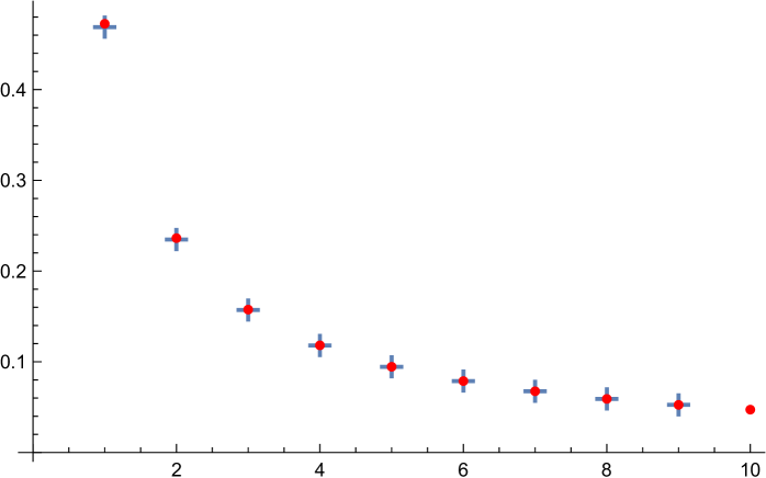
Fig. 11: The values of $\epsilon$ at the pitchfork bifurcations, as a function of $n$. Equation (35) is valid in the limit $\epsilon\rightarrow 0$, corresponding to $n\rightarrow\infty$. Crosses indicate numerical results, circles the asymptotic approximation.

In Figure 11 we show the values of $\epsilon$ at the pitchfork bifurcations as a function of $n$. Although the asymptotic approximation is valid as $n\rightarrow\infty$, the agreement with the numerical solution is remarkably good even at small $n$.

From (32) and (36) we see that the separation between the fold and pitchfork bifurcations is approximately

$$\frac{0.3943}{n^{3}}$$

as $n\rightarrow\infty$, and that the proportion of values of $\epsilon$ for which there are $4N+2$ solutions rather than $4N$ solutions therefore shrinks as $3.737\epsilon^{2}$ as $\epsilon\rightarrow 0$.

Fig. 12: Symmetric Solutions. The curves $n\pm X_{0}$ (black) and $n+1/2\pm X_{0}$ (blue) as a function of $k$ for $n=6$, $7$. The green curve is $\phi(1)/\epsilon$ with $\epsilon=0.0335$. The intersection points, highlighted, correspond to symmetric solutions of the problem. The lower and upper envelopes of the individual solutions are the curves $Y_{1}(A(x),x)$ and $Y_{2}(A(x),x)$ respectively.

Fig. 13: Non-symmetric Solutions. The curves $n\pm X_{0}$ (black) and $n+1/2\pm X_{0}$ (blue) as a function of $k$ for $n=6$, $7$. The green curve is $\phi(1)/\epsilon$ with $\epsilon=0.0335$. The intersection points of the green curve with integer and half-integer values, highlighted, correspond to non-symmetric solutions of the problem. The distance of these intersection points to the nearest black curve give the (signed) value of $\mu$. The lower and upper envelopes of the individual solutions are the curves $Y_{1}(A(x),x)$ and $Y_{2}(A(x),x)$ respectively.

3.6 Solutions with turning points

Thus far we have analysed solutions in which the Kuzmak approximation is valid all the way up to the boundary, which enabled us to capture quite well the structure of the bifurcation diagram shown in Figure 2. We now complete our asymptotic analysis by considering those solutions with turning points, in which the oscillations are confined to an interior region.

Suppose there are turning points at $\pm x^{*}$ (with $x^{*}>0$), so that $A(x^{*})=A_{1}(x^{*})$. For $|x|>x^{*}$ the solution does not oscillate, and (outside the boundary layers) $y_{0}$ is simply given by the outer solution (2):

$$y_{\mathrm{out}}(x)=-1+x^{2}-\sqrt{x^{4}-2x^{2}+2},\qquad|x|>x^{*}.$$ (37)

In this case $k$ is determined (at leading order) by the condition that

$$\mathchoice{\frac{{\partial}Y}{{\partial}X}}{{\partial}Y/{\partial}X}{{\partial}Y/{\partial}X}{{\partial}Y/{\partial}X}=0$$ (38)

at $x=x^{*}$, with $Y$ negative, so that the oscillating solution can join smoothly onto the non-oscillating solution. Note that continuity in the solution is automatic, since at the turning point $Y=Y_{1}=Y_{0}$, so that $Y$ is a root of both the cubic $c(Y)$ and also its derivative. Since, from (13)-(14), $\mathchoice{\frac{{\partial}Y}{{\partial}X}}{{\partial}Y/{\partial}X}{{\partial}Y/{\partial}X}{{\partial}Y/{\partial}X}=0$ (and $Y$ is negative) when $X=0$, equation (38) gives

$$\frac{\phi(x^{*})}{\epsilon}+\mu=n,\qquad-\frac{\phi(x^{*})}{\epsilon}+\mu=m.$$ (39)

Thus we are forced to choose either $\mu=0$ or $\mu=1/2$: the central part of the solutions is symmetric for all solutions with turning points. Note that

$$\phi^{\prime}\sim\frac{a}{\log(x-x^{*})},$$

for some constant $a$ as the turning point is approached with the result that the separation between spikes is $O(\epsilon\log\epsilon)$ there, in agreement with the analysis in [15] on the two spike solution.

Fig. 14: Solutions with turning points. The green curve is $\phi(x^{*})/\epsilon$ with $\epsilon=0.0335$ and $x^{*}$ satisfying $A(x^{*})=A_{1}(x^{*})$, shown as a function of $k$. The intersection points with integer and half-integer values, highlighted, correspond to solutions of the problem. Each point gives four distinct solutions, corresponding to the four combinations of boundary layers at $x=\pm 1$. The lower and upper envelopes of the individual solutions are the curves $Y_{1}(A(x),x)$ and $Y_{2}(A(x),x)$ respectively. Each solution plot shows both boundary layer possibilities at each end. For $n=6$ and $n=5.5$ the turning point is in the boundary layer, with the result that our approximation there is inaccurate.

As described in the introduction, the outer solution (37) does not satisfy the boundary conditions at $x=\pm 1$, where there are boundary layers. A uniform approximation valid for $|x|>x^{*}$ is

$$y \sim -1+x^{2}-\sqrt{2-2x^{2}+x^{4}}+3\,\mathrm{sech}^{2}\left(\pm\frac{(1-x)}{\epsilon\sqrt{2}}+\tanh^{-1}\left(\sqrt{\frac{2}{3}}\right)\right)$$

$$\mbox{ }+3\,\mathrm{sech}^{2}\left(\pm\frac{(1+x)}{\epsilon\sqrt{2}}+\tanh^{-1}\left(\sqrt{\frac{2}{3}}\right)\right).$$

In Figure 14 we show the solutions for $\epsilon=0.0335$, for which $\phi(x^{*})/\epsilon$ may take any integer or half-integer value up to $n=6$. The discontinuity in the gradient of the solution at $x=\pm x^{*}$ in these plots is due to the fact that we imposed continuity of the derivative only at leading order in $\epsilon$ there, using (38). Full continuity of the derivative implies

$$\mathchoice{\frac{\mathrm{d}y_{\mathrm{out}}}{\mathrm{d}x}}{\mathrm{d}y_{\mathrm{out}}/\mathrm{d}x}{\mathrm{d}y_{\mathrm{out}}/\mathrm{d}x}{\mathrm{d}y_{\mathrm{out}}/\mathrm{d}x}=\mathchoice{\frac{\mathrm{d}Y}{\mathrm{d}x}}{\mathrm{d}Y/\mathrm{d}x}{\mathrm{d}Y/\mathrm{d}x}{\mathrm{d}Y/\mathrm{d}x}=\frac{\Phi}{\epsilon}\mathchoice{\frac{{\partial}Y}{{\partial}X}}{{\partial}Y/{\partial}X}{{\partial}Y/{\partial}X}{{\partial}Y/{\partial}X}+\mathchoice{\frac{{\partial}Y}{{\partial}x}}{{\partial}Y/{\partial}x}{{\partial}Y/{\partial}x}{{\partial}Y/{\partial}x}+\mathchoice{\frac{{\partial}Y}{{\partial}\Phi}}{{\partial}Y/{\partial}\Phi}{{\partial}Y/{\partial}\Phi}{{\partial}Y/{\partial}\Phi}\left(\mathchoice{\frac{{\partial}\Phi}{{\partial}x}}{{\partial}\Phi/{\partial}x}{{\partial}\Phi/{\partial}x}{{\partial}\Phi/{\partial}x}+\mathchoice{\frac{{\partial}\Phi}{{\partial}A}}{{\partial}\Phi/{\partial}A}{{\partial}\Phi/{\partial}A}{{\partial}\Phi/{\partial}A}\mathchoice{\frac{\mathrm{d}A}{\mathrm{d}x}}{\mathrm{d}A/\mathrm{d}x}{\mathrm{d}A/\mathrm{d}x}{\mathrm{d}A/\mathrm{d}x}\right)+\mathchoice{\frac{{\partial}Y}{{\partial}A}}{{\partial}Y/{\partial}A}{{\partial}Y/{\partial}A}{{\partial}Y/{\partial}A}\mathchoice{\frac{\mathrm{d}A}{\mathrm{d}x}}{\mathrm{d}A/\mathrm{d}x}{\mathrm{d}A/\mathrm{d}x}{\mathrm{d}A/\mathrm{d}x},$$

which would introduce an $O(\epsilon)$ correction into equations (39). Each solution curve in Figure 14 shows four distinct solutions overlaid, corresponding to the four combinations of boundary layers at $x=\pm 1$.

These 48 solutions, together with the 8 solutions shown previously in Figures 12 and 13, make up the 56 solutions to the problem when $\epsilon=0.0335$.

4 Conclusion

The computational and asymptotic analysis we have presented gives a novel and complete taxonomy of the solutions of Carrier’s problem (1).

Using deflated continuation we found a rather striking bifurcation diagram, containing an apparently infinite number of mutually disconnected components. Each component (except for the first two) contains one fold bifurcation, at which two solutions of (1) appear, and one pitchfork bifurcation, at which a further two solutions of (1) appear. Solutions on the same connected component have the same number of interior maxima. For values of $\epsilon$ which do not lie between the fold and pitchfork bifurcations of a connected component the number of solutions of (1) is a multiple of 4, as claimed by Bender & Orszag [3]. However, between the fold and pitchfork bifurcations the number of solutions is $4n+2$ with $n\in{\mathbb{Z}}$.

Our asymptotic analysis used Kuzmak’s method to construct approximate solutions of (1). Both the fold and pitchfork bifurcation points were predicted accurately. We found that the separation between these bifurcation points tends quickly to zero as $\epsilon\rightarrow 0$, so that the proportion of values of $\epsilon$ for which there are $4n+2$ solutions rather than $4n$ solutions tends to zero as $3.737\epsilon^{2}$ as $\epsilon\rightarrow 0$.

We gave an alternative derivation of the result of Wong and Zhao that the maximum number of internal maxima is asymptotically

$$\left\lfloor\frac{0.472537}{\epsilon}\right\rfloor.$$

Moreover, we found that approximately 12% of solutions of the problem have oscillations which fill the domain. The remaining 88% of solutions have oscillations in an interior region near $x=0$ separated from boundary layers by a non-oscillating outer solution.

The methods we have used are in no way specific to (1). Carrier’s problem provides a nice example, but any slowly-varying phase plane with closed orbits would be amenable to our approach.

Appendix A Parameter values of the initial bifurcations

In the interest of completeness we tabulate the values of $\epsilon$ at which the first four pitchfork and fold bifurcations occur. The solution and parameter value at which a simple bifurcation occurs satisfy an augmented system of integro-differential equations [16]:

$$F(y,v,\epsilon)=\begin{bmatrix}\epsilon^{2}y^{\prime\prime}+2(1-x^{2})y+y^{2}-1\\ \epsilon^{2}v^{\prime\prime}+2(1-x^{2})v+2yv\\ \|v\|^{2}-1\end{bmatrix}=0,$$ (40)

where $y$ is the solution at the bifurcation point, $v$ is the eigenfunction in the nullspace of the Fréchet derivative of the equation, $\epsilon$ is the value of the parameter at the bifurcation, and $\|\cdot\|$ denotes the $L^{2}([-1,1])$ norm.

As we wish to compute the parameter values to high accuracy, a spectral discretization was chosen to approximate the solutions of (40). We thus employed the Chebfun system of Trefethen and co-workers [8, 4]. Solving (40) can be rather difficult, and the main art in its solution is the construction of good initial guesses for $(y,v,\epsilon)$. These were computed as follows.

For each bifurcation, an initial guess $(\tilde{y},\tilde{\epsilon})$ for the solution and parameter was acquired from the data produced by deflated continuation. The finite element solution $\tilde{y}$ was evaluated at 200 Chebyshev points of the second kind and its Chebyshev interpolant $\mathcal{I}\tilde{y}$ was constructed with Chebfun. Carrier’s problem at $\epsilon=\tilde{\epsilon}$ was then solved with this initial guess, yielding $\hat{y}$, to ensure that the first equation of (40) had small residual. The differential operator was linearized at $(\hat{y},\tilde{\epsilon})$ to compute its eigenfunction $\hat{v}$ with eigenvalue closest to zero; this ensured that the second and third equations had small residual. The triplet $(\hat{y},\hat{v},\tilde{\epsilon})$ was then supplied as initial guess to the solver for (40). The fold bifurcations typically converged in four or five Newton iterations, while the pitchfork bifurcations typically converged in twenty to thirty iterations. In all cases Chebfun’s error estimate for the solution of (40) was less than $10^{-10}$; no further accuracy was possible due to the use of double precision arithmetic.

Connected	Computed	Asymptotic	Relative
component	$\epsilon$	estimate	error
1	0.46886251	0.472537	0.007837
2	0.23472529	0.236269	0.006574
3	0.15703946	0.157512	0.003012
4	0.11798359	0.118134	0.001278

Table 1: Computed parameter values for the first four pitchfork bifurcations. The asymptotic estimates are those of (36).

Connected	Computed	Asymptotic	Relative
component	$\epsilon$	estimate	error
2	0.28522538	0.298545	0.0467
3	0.17186970	0.173608	0.01011
4	0.12421206	0.124634	0.003397
5	0.09762446	0.0977706	0.001497

Table 2: Computed parameter values for the first four fold bifurcations. The asymptotic estimates are those of (32).

Appendix B Approximation for large $\epsilon$

For completeness we give here an asymptotic approximation to the two solutions which continue to exist when $\epsilon$ is large. Expanding $y$ in an inverse power series in $\epsilon$ as

$$y\sim y_{0}+\epsilon^{-2}y_{1}+\cdots,$$

gives at leading order

$$y_{0}^{\prime\prime}=0,\qquad y_{0}(-1)=y_{0}(1)=0,$$

with solution $y_{0}\equiv 0$, indicating that $y$ is not $O(1)$ but must be rescaled in some way. Expanding

$$y\sim\epsilon^{-2}y_{0}+\epsilon^{-4}y_{1}+\cdots,$$

gives at leading order

$$y_{0}^{\prime\prime}=1,\qquad y_{0}(-1)=y_{0}(1)=0,$$

with solution

$$y_{0}=\frac{x^{2}-1}{2}.$$

This solution has no internal maximum, and is the continuation to large $\epsilon$ of the solution in panel $1$ of Fig 2.

The second solution is found by expanding $y$ as

$$y\sim\epsilon^{2}y_{0}+y_{1}+\cdots,$$

to give at leading order

$$y_{0}^{\prime\prime}+y_{0}^{2}=0,\qquad y_{0}(-1)=y_{0}(1)=0,$$

with solution

$$1+x=\frac{\sqrt{3}}{\sqrt{2}}\int_{0}^{y}\frac{\mathrm{d}u}{(y_{\mathrm{max}}^{3}-u^{3})^{1/2}},$$

where $y_{\mathrm{max}}$, the value of $y$ at $x=0$, satisfies

$$1=\frac{\sqrt{3}}{\sqrt{2}}\int_{0}^{y_{\mathrm{max}}}\frac{\mathrm{d}u}{(y_{\mathrm{max}}^{3}-u^{3})^{1/2}}=\sqrt{\frac{3\pi}{2y_{\mathrm{max}}}}\frac{\Gamma(4/3)}{\Gamma(5/6)},$$

so that

$$y_{\mathrm{max}}=\frac{3\pi\Gamma(4/3)^{2}}{2\Gamma(5/6)^{2}}.$$

This solution has one internal maximum, and is the continuation to large $\epsilon$ of the solution in panel $2$ of Fig 2.

References

- [1] S. Ai, Multi-bump solutions to Carrier’s problem, J. Math. Anal. Appl., 277 (2003), pp. 405–422.
- [2] S. Balay et al., PETSc users manual, Tech. Report ANL-95/11 - Revision 3.6, Argonne National Laboratory, 2015.
- [3] C. M. Bender and S. A. Orszag, Advanced Mathematical Methods for Scientists and Engineers I: Asymptotic Methods and Perturbation Theory, Springer, 1999.
- [4] Á. Birkisson and T. A. Driscoll, Automatic Fréchet differentiation for the numerical solution of boundary-value problems, ACM Transactions on Mathematical Software, 38 (2012), pp. 26:1–26:29.
- [5] G. F. Carrier, Singular perturbation theory and geophysics, SIAM Review, 12 (1970), pp. 175–193.
- [6] G. F. Carrier and C. Pearson, Ordinary Differential Equations, vol. 6 of Classics in Applied Mathematics, SIAM, 1985.
- [7] E. Doedel and J. P. Kernévez, AUTO: Software for continuation and bifurcation problems in ordinary differential equations, tech. report, California Institute of Technology, 1986.
- [8] T. A Driscoll, N. Hale, and L. N. Trefethen, Chebfun Guide, Pafnuty Publications, 2014.
- [9] P. E. Farrell, C. H. L. Beentjes, and Á. Birkisson, The computation of disconnected bifurcation diagrams, 2016. arXiv:1603.00809 [math.NA].
- [10] W. L. Kath, Slowly varying phase planes and boundary-layer theory, Stud. Appl. Math., 72 (1972), pp. 221–239.
- [11] H. B. Keller, Numerical solution of bifurcation and nonlinear eigenvalue problems, in Applications of Bifurcation Theory, P. H. Rabinowitz, ed., New York, 1977, Academic Press, pp. 359–384.
- [12] G. E. Kuzmak, Asymptotic solutions of nonlinear second order differential equations with variable coefficients, J. Appl. Math. Mech., 23 (1959), pp. 730–744.
- [13] L. D. Landau and E. M. Lifshitz, Mechanics, Pergamon, 3rd ed., 1976.
- [14] A. Logg, K. A. Mardal, G. N. Wells, et al., Automated Solution of Differential Equations by the Finite Element Method, Springer, 2011.
- [15] A. D. MacGillivray, R. J. Braun, and G. Tanoğlu, Perturbation analysis of a problem of Carrier’s, Stud. Appl. Math., 104 (2000), pp. 293–311.
- [16] G. Moore and A. Spence, The calculation of turning points of nonlinear equations, SIAM Journal on Numerical Analysis, 17 (1980), pp. 567–576.
- [17] R. Wong and Y. Zhao, On the number of solutions to Carrier’s problem, Studies in Applied Mathematics, 120 (2008), pp. 213–245.