Constraining the Galactic structure parameters with the XSTPS-GAC and SDSS photometric surveys

Abstract

Photometric data from the Xuyi Schmidt Telescope Photometric Survey of the Galactic Anticentre (XSTPS-GAC) and the Sloan Digital Sky Survey (SDSS) are used to derive the global structure parameters of the smooth components of the Milky Way. The data, which cover nearly 11,000 deg² sky area and the full range of Galactic latitude, allow us to construct a globally representative Galactic model. The number density distribution of Galactic halo stars is fitted with an oblate spheroid that decays by power law. The best-fit yields an axis ratio and a power law index $\kappa=0.65$ and $p=2.79$, respectively. The $r$-band differential star counts of three dwarf samples are then fitted with a Galactic model. The best-fit model yielded by a Markov Chain Monte Carlo analysis has thin and thick disk scale heights and lengths of $H_{1}=$ 322 pc and $L_{1}=$2343 pc, $H_{2}=$794 pc and $L_{2}=$3638 pc, a local thick-to-thin disk density ratio of $f_{2}=$11 per cent, and a local density ratio of the oblate halo to the thin disk of $f_{h}=$0.16 per cent. The measured star count distribution, which is in good agreement with the above model for most of the sky area, shows a number of statistically significant large scale overdensities, including some of the previously known substructures, such as the Virgo overdensity and the so-called “north near structure”, and a new feature between 150°$<l<$ 240° and $-1$5°$<b<$ $-$5°, at an estimated distance between 1.0 and 1.5 kpc. The Galactic North-South asymmetry in the anticentre is even stronger than previously thought.

1 Introduction

One of the fundamental tasks of the Galactic studies is to estimate the structure parameters of the major structure components. Bahcall & Soneira (1980) fit the observations with two structure components, namely a disk and a halo. Gilmore & Reid (1983) introduce a third component, namely a thick disk, confirmed in the earliest Besancon Galaxy Model Crézé & Robin (1983). Since then, various methods and observations have been adopted to estimate parameters of the thin and thick disks and of the halo of our Galaxy. As the quantity and quality of data available continue to improve over the years, the model parameters derived have become more precise, numerically. Ironically, those numerically more precise results do not converge (see Table 1 of Chang et al. 2011, Table 2 of López-Corredoira & Molgó 2014 and Sect. 5 and 6 of Bland-Hawthorn & Gerhard 2016 for a review). The scatters in density law parameters, such as scale lengths, scale heights and local densities of these Galactic components, as reported in the literature, are rather large. At least parts of the discrepancies are caused by degeneracy of model parameters, which in turn, can be traced back to the different data sets adopted in the analyses. Those differing data sets either probe different sky areas (Bilir et al., 2006a; Du et al., 2006; Cabrera-Lavers et al., 2007; Ak et al., 2007; Yaz & Karaali, 2010; Yaz Gökçe et al., 2015), are of different completeness magnitudes and therefore refer to different limiting distances (Karaali et al., 2007), or of consist of stars of different populations of different absolute magnitudes (Karaali et al., 2004; Bilir et al., 2006b; Jurić et al., 2008; Jia et al., 2014). It should be noted that the analysis of Bovy et al. (2012), using the SEGUE spectroscopic survey, has given a new insight on the thin and thick disk structural parameters. This analysis provides estimate of their scale height and scale height as a function of metallicity and alpha abundance ratio. However, it relies on incomplete data (since it is spectroscopic) with relatively low range of Galactocentric radius as for the thin disk is concerned.

A wider and deeper sample than those employed hitherto may help break the degeneracy inherent in a multi-parameter analysis and yield a globally representative Galactic model. A single or a few fields are insufficient to break the degeneracy. The resulted best-fit parameters, while sufficient for the description of the lines of sight observed, may be unrepresentative of the entire Galaxy. For the latter purpose, systematic surveys of deep limiting magnitude of all or a wide sky area, such as the Two Micron All Sky Survey (2MASS; Skrutskie et al. 2006), the Sloan Digital Sky Survey (SDSS; York et al. 2000), the Panoramic Survey Telescope & Rapid Response System (Pan-Starrs; Kaiser et al. 2002) and the GAIA mission (Perryman et al., 2001), are always preferred.

Several authors have studied the Galactic structure with 2MASS data at low (López-Corredoira et al., 2002; Yaz Gökçe et al., 2015) or high latitudes (Cabrera-Lavers et al., 2005, 2007; Chang et al., 2011). Polido et al. (2013) uses the model from Ortiz & Lepine (1993) and rederive the parameters of this model based on the 2MASS star counts over the whole sky area. However, the survey depth of 2MASS is not quite enough to reach the outer disk and the halo. The survey depth of SDSS is much deeper than that of the 2MASS. Many authors (e.g. Chen et al. 2001; Bilir et al. 2006a, 2008; Jia et al. 2014; López-Corredoira & Molgó 2014) have previously used the SDSS data to constrain the Galactic parameters. Those authors have only made use of a portion of the surveyed fields, at intermediate or high Galactic latitudes. Jurić et al. (2008) obtain Galactic model parameters from the stellar number density distribution of 48 million stars detected by the SDSS that sample distances from 100 pc to 20 kpc and cover 6500 deg² of sky. Their results are amongst those mostly quoted. However, in their analysis, they have avoided the Galactic plane. So the constraints of their results on the disks, especially the thin disk, are weak. In their analysis, Jurić et al. (2008) have also adopted photometric parallaxes assuming that all stars of the same colour have the same metallicity. Clearly, (disk) stars in different parts of the Galaxy have quite different (Ivezić et al., 2008; Xiang et al., 2015; Huang et al., 2015) metallicities, and these variations in metallicities may well lead to biases in the model parameters derived.

In order to provide a quality input catalog for the LAMOST Spectroscopic Survey of the Galactic Anticentre (LSS-GAC; Liu et al. 2014, 2015; Yuan et al. 2015b), a multi-band CCD photometric survey of the Galactic Anticentre with the Xuyi 1.04/1.20m Schmidt Telescope (XSTPS-GAC; Zhang et al. 2013, 2014; Liu et al. 2014) has been carried out. The XSTPS-GAC photometric catalog contains more than 100 million stars in the direction of Galactic anticentre (GAC). It provides an excellent data set to study the Galactic disk, its structures and substructures. In this paper, we take the effort to constrain the Galactic model parameters by combining photometric data from the XSTPS-GAC and SDSS surveys. This is the third paper of a series on the Milky Way study based on the XSTPS-GAC data. In Chen et al. (2014), we present a three dimensional extinction map in $r$ band. The map has a spatial angular resolution, depending on latitude, between 3 and 9 arcmin and covers the entire XSTPS-GAC survey area of over 6,000 deg² for Galactic longitude 140 $<l<$220 deg and latitude 40 $<b<$40 deg. In Chen et al. (2015), we investigate the correlation between the extinction and the $\rm H~{}{\scriptstyle I}$  and CO emission at intermediate and high Galactic latitudes ($|b|>$ 10°) within the footprint of the XSTPS-GAC, on small and large scales. In the current work we are interested in the global, smooth structure of the Galaxy.

For the Galactic structure, in addition to the global, smooth major components, many more (sub-)structures have been discovered, including the inner bars near the Galactic centre (Alves, 2000; Hammersley et al., 2000; van Loon et al., 2003; Nishiyama et al., 2005; Cabrera-Lavers et al., 2008; Robin et al., 2012), flares and warps of the (outer) disk (López-Corredoira et al., 2002; Robin et al., 2003; Momany et al., 2006; Reylé et al., 2009; López-Corredoira & Molgó, 2014), and various overdensities in the halo and the outer disk, such as the Sagittarius Stream (Majewski et al., 2003), the Triangulum-Andromeda (Rocha-Pinto et al., 2004; Majewski et al., 2004) and Virgo (Jurić et al., 2008) overdensities, the Monoceros ring (Newberg et al., 2002; Rocha-Pinto et al., 2003) and the Anti-Center Stream (Rocha-Pinto et al., 2003; Crane et al., 2003; Frinchaboy et al., 2004). They show the complexity of the Milky Way. Recently, Widrow et al. (2012) and Yanny & Gardner (2013) have found evidence for a significant Galactic North-South asymmetry in the stellar number density distribution, exhibiting some wavelike perturbations that seem to be intrinsic to the disk. Xu et al. (2015) show that in the anticentre regions there is an oscillating asymmetry in the main-sequence star counts on either sides of the Galactic plane, in support of the prediction of Ibata et al. (2003). The asymmetry oscillates in the sense that there are more stars in the north, then in the south, then back in the north, and then back in the south at distances of about 2, 4 – 6, 8 – 10 and 12 – 16 kpc from the Sun, respectively.

The paper is structured as follows. The data are introduced in Section 2. We describe our model and the analysis method in Section 3. Section 4 presents the results and discussions. In Section 5 we discuss the large scale excess/deficiency of star counts that reflect the substructures in the halo and disk. Finally we give a summary in Section 6.

2 Data

Table 1: Data sets.

	area	field size	$N_{\rm fields}$	$r$ ranges
	(deg2)	(deg $\times$ deg)		(mag)
XSTPS-GAC	$\sim$3392	2.5$\times$2.5	574	12–18
XSTPS-M31/M33	$\sim$588	2.5$\times$2.5	108	12–18
SDSS	$\sim$6871	3.0$\times$3.0	1592	15–21

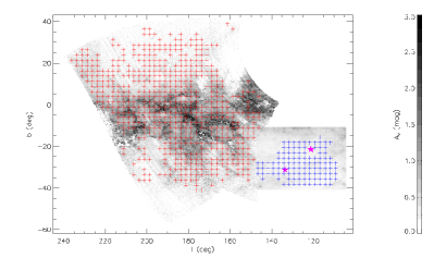
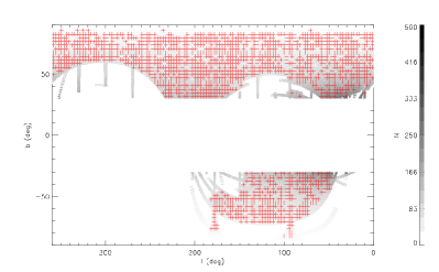
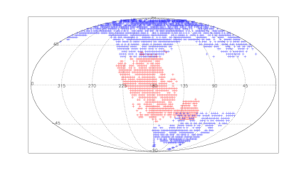
Figure 1: Upper panel: Extinction map of the GAC and M31/M33 areas within the footprint of XSTPS-GAC (Chen et al. 2015 map for GAC area and Schlegel et al. 1998 map for M31/M33 area). The selected fields for GAC area and M31/M33 area are marked as red and blue pluses, respectively. The red star symbols mark the central positions of M31 and M33, respectively. Middle panel: SDSS DR12 density map of stars in a magnitude bin of $r$ = 15.5 to 16.5 mag at a resolution of 0.1°. The selected fields from SDSS are marked as red pluses. Bottom panel: Location of the 682 fields selected from the XSTPS-GAC (red) and 1592 fields selected from the SDSS (blue) in Galactic coordinates.

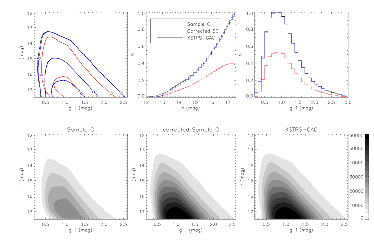
Figure 2: Colour-magnitude distributions of stars in all selected subfields from the Sample C, the re-weighted Sample C (see Equation (1) and related discussion), and the XSTPS-GAC. The bottom three panels show the grey-scaled number densities distributed in the $g-i$ vs. $r$ space respectively for the XSTPS-GAC (left), the re-weighted Sample C (middle), and the XSTPS-GAC (right). The upper three panels show the number distribution contours in the $g-i$ vs. $r$ space (left) as well as number distributions respectively in $r$ (middle) and $g-i$ (right) for each sample. The black contours and histograms show the density of all targets in the XSTPS-GAC, the red ones represent the distributions of stars in Sample C and the blue ones display the distributions for the re-weighted Sample C. The contours labeled with ‘a’, ‘b’ and ‘c’ in the left-upper panel represent the contour levels of star number of 6 000, 24 000 and 48 000, respectively. The re-weighted Sample C perfectly reproduces the colour-magnitude sampling provided by the XSTPS-GAC.

2.1 The XSTPS-GAC Data

The XSTPS-GAC started collecting data in the fall of 2009 and completed in the spring of 2011. It was carried out in order to provide input catalogue for the LSS-GAC. The survey was performed in the SDSS $g$, $r$ and $i$ bands using the Xuyi 1.04/1.20 m Schmidt Telescope equipped with a 4k$\times$4k CCD camera, operated by the Near Earth Objects Research Group of the Purple Mountain Observatory. The CCD offers a field of view (FoV) of 1.94°$\times$ 1.94°, with a pixel scale of 1.705 arcsec. In total, the XSTPS-GAC archives approximately 100 million stars down to a limiting magnitude of about 19 in $r$ band ($\sim$ 10$\sigma$) with an astrometric accuracy about 0.1 arcsec and a global photometric accuracy of about 2% (Liu et al., 2014). The total survey area of XSTPS-GAC is close to 7,000 deg², covering an area of $\sim$ 5,400 deg² centered on the GAC, from RA $\sim$ 3 to 9 h and Dec $\sim~{}-$10°to $+60\degr$, plus an extension of about 900 deg² to the M31/M33 area and the bridging fields connecting the two areas.

2.1.1 GAC area

In the direction of GAC, the $r$-band extinction exceeds 1 mag over a significant fraction of the sky (see Fig. 1). To correct the extinction of stars in high extinguish area using extinction maps integrated over lines of sight, such as Schlegel et al. (1998), will introduce over corrections. It will make stars too bright and blue. We select a subsample, the so-called “Sample C” in Chen et al. (2014), from XSTPS-GAC. Extinction of all stars in Sample C were calculated by the spectral energy distribution (SED) fitting to the multi-band data, including the photometric data from the optical ($g,~{}r,~{}i$ from XSTPS-GAC) to the near-infrared ($J,~{}H,~{}K_{S}$ from 2MASS and $W1,~{}W2$ from the Wide-field Infrared Survey Explorer, WISE, Wright et al. 2010). The extinction of targets in the subsample, Sample C, is highly reliable, all having minimum SED fitting $\chi^{2}_{min}~{}<$ 2.0 (see Chen et al. 2014 for more details). We correct the extinction of stars in Sample C using the SED fitting extinction and the extinction law from Yuan et al. (2013). There are more than 13 million stars in Sample C. We divide them into small subfields of roughly 2.5°$\times$ 2.5°. The width ($\Delta l$) and height ($\Delta b$) of each subfield are always exactly 2.5°. Each subfield is not exactly 6.25 deg² but varies with Galactic latitude $b$. Because of the heavy extinction or poor observational conditions (large photometric errors), some subfields have obviously small amount of stars, comparing to most normal neighboring fields and thus be excluded. As a result, 574 subfields, covering about 3392 deg², are selected. The locations of these subfields are shown in the top panel of Fig. 1, with the grey-scale background image illustrating the 4 kpc extinction map from Chen et al. (2015).

For each subfield, Sample C does not contain all stars in XSTPS-GAC. To connect the distribution of targets in Sample C to the underlying distribution of all stars, it is necessary to correct for the effects of the selection (often referred to as selection biases). Generally, the selection effects of Sample C are due to the following two reasons: (1) the procedure by which we cross-match the photometric catalogue of the XSTPS-GAC with those of 2MASS and WISE, and (2) the $\chi^{2}$ cut when we define the sample with highly reliable extinction estimates. For the first part, we lose about 15 per cent objects, mainly due to the limiting depths of 2MASS and WISE, especially at low Galactic latitudes (see Fig. 1 of Chen et al. 2014). For the second part, we lose more than half of the objects, because of the large photometric errors, high extinction effects, or the special targets contamination, such as blended or binaries which are not well fitted by the standard SED library in Chen et al. (2014). Our model for the selection function of Sample C can thus be expressed as the function of the positions ($l$, $b$), colour ($g-i$) and magnitude ($r$) of stars, given by,

$$S(l,b,g-i,r)=\frac{N_{\rm SC}(l,b,g-i,r)}{N_{\rm XSTPS}(l,b,g-i,r)},$$ (1)

where $N_{\rm SC}(l,b,g-i,r)$ and $N_{\rm XSTPS}(l,b,g-i,r)$ are the number of stars in the Sample C and the XSTPS-GAC, respectively. The numbers of objects are evaluated within each subfield with area of $\sim$ 6.25 deg², each colour ($g-i$) bin ranging from 0 to 3.0 mag with a bin-size of 0.1 mag, and each $r$-band magnitude bin ranging from 12 to 18.5 mag with a bin-size of 0.1 mag.

The number distributions in colour $(g-i)$ and magnitude $r$ for the stars in all selected subfields in the Sample C, the Sample C re-weighted by the selection effect, as well as the XSTPS-GAC, are shown as the density grey-scales and density contours and histograms in Fig. 2. It is clear that our correction of selection effect leads to perfect agreement between the complete XSTPS-GAC photometric sample and the re-weighted Sample C.

2.1.2 M31/M33 area

The dust extinction in the M31 and M33 area is much smaller, compared with the GAC area (see the top panel of Fig. 1). We adopt the extinction map from Schlegel et al. (1998) and the extinction law from Yuan et al. (2013) to correct the extinction of stars in M31/M33 area. Similarly as in the GAC area, all stars in M31/M33 area are divided into small subfields, which have width ($\Delta l$) and height ($\Delta b$) always of 2.5°. We exclude the subfields which have maximum $E(B-V)$ larger than 0.15 mag (i.e. $A_{r}$ = 0.4 mag, according to the extinction law from Yuan et al. 2013), to avoid the relatively large uncertainties caused by the high extinction in the highly extinguished regions. The subfields that cover M31 are also excluded. As a result, there are 108 subfields in the M31/M33 area, covering about 588 deg². The locations of these subfields are also plotted in the top panel of Fig. 1, with the grey-scale background image illustrating the extinction map from Schlegel et al. (1998). Considering the limiting magnitude of XSTPS-GAC ($r$ $\sim$ 19 mag), we claim that the data in the M31/M33 area from XSTPS-GAC is complete in the magnitude range $12<r_{0}<18$ mag.

2.2 The SDSS Data

As the survey area of XSTPS-GAC mainly locate around the low Galactic latitudes, we also use the photometric data from SDSS, for constraining better the outer disk and the halo. We use the photometric data from SDSS data release 12 (DR12, Alam et al. 2015). The SDSS surveys mainly for high Galactic latitudes, with only a few stripes crossing the Galactic plane. It complements one another with the XSTPS-GAC. We cut the SDSS data with Galactic latitude $|b|>$ 30°, where the influence of the dust extinction is small. The dust extinction are corrected using the extinction map from Schlegel et al. (1998) and the extinction law from Yuan et al. (2013). The SDSS data are divided into subfields with width ($\Delta l$) and height ($\Delta b$) always of 3°. To make sure that each subfield is fully sampled by the SDSS survey, we further divide each subfield into smaller pixels (of size 0.1°$\times$ 0.1°) and exclude the subfield which has no stars detected in at least one of the smaller pixels. As a result we have obtained 1592 subfields, covering a sky area of about 6871 deg². In the middle panel of Fig. 1, we show the spatial distributions of these subfields, with grey-scale background image illustrating the number density of the SDSS data. To remove the contaminations of hot white dwarfs, low-redshift quasars and white dwarf/red dwarf unresolved binaries from the SDSS sample, we reject objects at distances larger than 0.3 mag from the $(r-i)_{0}$ vs. $(g-r)_{0}$ stellar loci (Jurić et al., 2008; Chen et al., 2014). The 95 per cent completeness limits of the SDSS images are $u$, $g$, $r$, $i$ and $z$ $=$ 22.0, 22.2, 22.2, 21.3 and 20.5 mag, respectively (Abazajian et al., 2004). Thus the SDSS data is complete in the magnitude range of $15<r_{0}<21$ mag.

A brief summary of the data selection in the current work is given in Table 1. In total, there are 2274 subfields, covering nearly 11,000 deg², which is more than a quarter of the whole sky area. The positions of all the subfields, from both the XSTPS-GAC and the SDSS, are plotted in the bottom panel of Fig. 1. They cover the whole range of Galactic latitudes. Generally, the XSTPS-GAC provides nice constraints of the Galactic disk(s), especially for the thin disk, while the SDSS provides us a good opportunity to refine the structure of Galactic halo, as well as the outer disk.

3 The Method

3.1 The Galactic model

We adopt a three-components model for the smooth stellar distribution of the Milky Way. It comprises two exponential disks (the thin disk and the thick disk) and a two-axial power-law ellipsoid halo (Bahcall & Soneira, 1980; Gilmore & Reid, 1983). Thus the overall stellar density $n(R,Z)$ at a location $(R,Z)$ can be decomposed by the sum of the thin disk, the thick disk and the halo,

$$n(R,Z)=D_{1}(R,Z)+D_{2}(R,Z)+H(R,Z),$$ (2)

where $R$ is the Galactocentric distance in the Galactic plane, $Z$ is the distance from the Galactic mid-plane. $D_{1}$ and $D_{2}$ are stellar densities of the thin disk and the thick disk,

$$D_{i}(R,Z)=f_{i}\,n_{0}\exp\left[-\,{(R-R_{\odot})\over L_{i}}-\,{(|Z|-Z_{\odot})\over H_{i}}\right],$$ (3)

where the suffix $i=1$ and $2$ stands for the thin disk and thick disk, respectively. $R_{\odot}$ is the radial distance of the Sun to the Galactic centre on the plane, $Z_{\odot}$ is the vertical distance of the Sun from the plane, $n_{0}$ is the local stellar number density of the thin disk at ($R_{\odot}$, $Z_{\odot}$), $f_{i}$ is the density ratio to the thin disk ($f_{1}$=1), $L_{i}$ is the scale-length and $H_{i}$ is the scale-height. We adopt $R_{\odot}=8$ kpc (Reid & Majewski, 1993) and $Z_{\odot}=25$ pc (Jurić et al., 2008) in the current work. $H$ is the stellar density of the halo,

$$H(R,Z)=f_{h}\,n_{0}\left[R^{2}+(Z/\kappa)^{2}\over R_{\odot}^{2}+(Z_{\odot}/\kappa)^{2}\right]^{-p/2},$$ (4)

where $\kappa$ is the axis ratio, $p$ is the power index and $f_{h}$ is the halo normalization relative to the thin disk.

3.2 Halo fit

Table 2: The parameter space and results of the halo fit

Parameters	Range	Grid size	Best value	Uncertainty
$\kappa$	0.1–1.0	0.01	0.65	0.05
$p$	2.3–3.3	0.01	2.79	0.17

We fit the component of the halo first. The metallicity distribution of the halo stars can be described as a single Gaussian component, with a median halo metallicity of $\mu_{\rm H}$=$-$1.46 dex and spatially invariant of $\sigma_{\rm H}$=0.30 dex (Ivezić et al., 2008). We assume the metallicity of all halo stars as [Fe/H]$=-1.46$ dex and adopt the photometric parallax relation from Ivezić et al. (2008),

$$\begin{split}M_{r}=&4.50-1.11{\rm[Fe/H]}-0.18{\rm[Fe/H]}^{2}\\ &-5.06+14.32(g-i)_{0}-12.97(g-i)_{0}^{2}\\ &+6.127(g-i)_{0}^{3}-1.267(g-i)_{0}^{4}+0.0967(g-i)_{0}^{5}.\end{split}$$ (5)

The distances of the halo stars can thus be calculated from the standard relation,

$$d=10^{0.2(r_{0}-M_{r})+1}.$$ (6)

Star in a blue colour bin $0.5\leq g-i<0.6$ are selected. They do not suffer from the giant star contamination and probe larger distances to constrain the halo. We calculate their distance using Equations (5) and (6). The distances of the disk stars will be underestimated because they are more metal-rich. To exclude the contamination of the disk stars, we use stars with absolute distance to the Galactic plane $|Z|>$ 4 kpc. For each subfield, we divide all halo stars into suitable numbers of logarithmic distance bins and then count the number for each bin. This number can be modelled as,

$$N_{\rm H}(d)=H(d)\Delta V(d),$$ (7)

where $H(d)$ is the halo stellar density given by Equation (4) and $\Delta V(d)$ is the volume, given by,

$$\Delta V(d)=\frac{\omega}{3}(\frac{\pi}{180})^{2}(d^{3}_{2}-d^{3}_{1}),$$ (8)

where $\omega$ denotes the area of the field (unit in deg²), $d_{1}$ and $d_{2}$ are the lower distance limit and upper distance limit of the bin, respectively.

We fit the halo model parameters $p$ and $\kappa$ to the data. As we explicitly exclude the disk, we cannot fit for the halo-to-thin disk normalization $f_{h}$. A maximum likelihood technique is adopted to explore the best values of those halo model parameters. In Table 2, we list the searching parameter space and the grid size. For each set of parameters, a reduced likelihood is computed between the simulated data (star counts in bins of distances) and the observations, given by Bienayme et al. (1987) and Robin et al. (2014),

$$Lr=\sum_{i=1}^{N}q_{i}\times(1-R_{i}+{\rm ln}(R_{i})),$$ (9)

where $Lr$ is the reduced likelihood for a binomial statistics, $i$ is the index of each distance bin, $f_{i}$ and $q_{i}$ are the number of stars in the $i$th bin for the model and the data, respectively and $R_{i}=f_{i}/q_{i}$. The uncertainties of the halo parameters are estimated similarly as those in Chang et al. (2011). We calculate the likelihood for 1000 times using the observed data and the simulations of the best-fit model adding with the Poisson noises. The resulted likelihood range defines the confidence level and thus the uncertainties.

3.3 Disk fit

The metallicity distribution of the disk is more complicated than that of the halo. Thus we fit the disk model parameters through a different way. We compare the $r$-band differential star counts in different colour bins and compare them to the simulations to search for the best disk model parameters ($n_{0},~{}L_{1},~{}H_{1},~{}f_{2},~{}L_{2}$ and $H_{2}$), as well as the halo-to-thin disk normalization $f_{h}$.

Towards a subfield of galactic coordinates ($l,~{}b$) and solid angle $\omega$, the $r$-band differential star counts $N_{\rm sim}(r^{k}_{0})$ ($k$ is the index of each magnitude bin) in a given colour bin $(g-i)^{j}_{0}$ ($j$ is the index of each colour bin) can be simulated as follows:

1. The line of sight is divided into many small distance bins. For a given distance bin with centre distance of $d_{i}$ ($i$ is the index of each distance bin), the $r$-band apparent magnitude of a star is given by

   $$r_{0}(d_{i})=M_{r}((g-i)^{j}_{0},{\rm[Fe/H]}|l,b,d_{i})+\mu,$$ (10)

   where $\mu$ is the distance modulus [$\mu=5{\rm log}_{10}(d_{i})-5$] and $M_{r}$ is the $r$-band absolute magnitude of the star given by Equation (5). The metallicities of halo stars are again assumed to be $-$1.46 dex and those of disk stars are given as a function of positions, which is fitted using the metallicities of main sequence turn off stars from LSS-GAC (Xiang et al., 2015),

   $${\rm[Fe/H]}=-0.61+0.51\cdot{\rm exp}{(-|Z|/1.57)}.$$ (11)

2. The number of stars in each distance bin can be calculated by,

   $$N(d_{i})=n(R,Z|l,b,d_{i})V(d_{i}),$$ (12)

   where $V(d_{i})$ is the volume given by Equation (8) and $n(R,Z|l,b,d_{i})$ is the stellar number density given by Equation (2, 3 and 4). The halo model parameters, $\kappa$ and $p$, resulted from the halo fit are adopted and settled to be not changeable here.

3. Combining all distance bins, we can obtain the modeled $r$-band star counts $N(r^{k}_{0})$, by

   $$N(r^{k}_{0})=\Sigma N(d_{i})~{}{\rm where}~{}r^{k}_{0}-\frac{\rm rbin}{2}<r_{0}(d_{i})<r^{k}_{0}+\frac{\rm rbin}{2},$$ (13)

   where rbin is the bin size of $r$-band magnitude (we adopt rbin=1 mag in the current work). $N(r^{k}_{0})$ is the underlying star counts. When comparing to the observations, we need to apply the selection function, by

   $$N_{\rm sim}(r^{k}_{0})=N(r^{k}_{0})S(l,b,g-i,r)C,$$ (14)

   where $S(l,b,g-i,r)$ is the selection function, calculated by Equation (1) for XSTPS-GAC subfields in GAC area and equals to one for XSTPS-GAC subfields in M31/M33 area and all the SDSS subfields. Besides,

   $$C=\begin{cases}1&{\rm for~{}}d_{\rm min}<d_{i}<d_{\rm max};\\ 0&{\rm otherwise};\\ \end{cases}$$ (15)

   $$d_{\rm min} = 10^{0.2(r_{\rm min}-A_{r}(d_{i})-M_{r}((g-i)_{0},{\rm[Fe/H]}))+1},$$ (16)

   $$d_{\rm max} = 10^{0.2(r_{\rm max}-A_{r}(d_{i})-M_{r}((g-i)_{0},{\rm[Fe/H]}))+1},$$ (17)

   where $r_{\rm min}$ and $r_{\rm max}$ are the magnitude limits of each subfield. We adopt $r_{\rm min}=12$ and $r_{\rm max}=18$ for all XSTPS-GAC subfields, and $r_{\rm min}=15$ and $r_{\rm max}=21$ for all SDSS subfields. $A_{r}(d_{i})$ is the extinction in $r$-band at distance of $d_{i}$. We adopt the 3D extinction map from Chen et al. (2014) for XSTPS-GAC subfields in GAC area and 2D extinction map from Schlegel et al. (1998) for XSTPS-GAC subfields in M31/M33 area and all SDSS subfields. As the size of each subfield is quite large ($\sim$ 4 deg²), the extinction $A_{r}(d)$ varies within a subfield. We thus adopt the maximum values to make sure that our data are complete.

The photometric parallax relation of Equation (5) is only valid for the single stars. A large fraction of stars in the Milky Way are actually binaries (e.g. Yuan et al. 2015a). In the current work we adopt the binary fraction resulted from Yuan et al. (2015a) and assume that 40 per cent of the stars are binaries. The absolute magnitudes $M_{r}$ of the binaries are calculated as the same way as in Yuan et al. (2015a).

We also consider the effects of photometric errors, the dispersion of disk star metallicities and the errors due to the photometric parallax relation of Ivezić et al. (2008). The $r$-band photometric errors of most stars in the XSTPS-GAC and the SDSS are smaller than 0.05 mag (Chen et al. 2014 for the XSTPS-GAC and Sesar et al. 2006 for the SDSS). When we fit the metallicities of disk stars as a function of positions [Equation (11)], we find a dispersion of the residuals of about 0.05 dex. According to Equation (5), this dispersion would introduce an offset of about 0.05 mag for the absolute magnitude when [Fe/H] = $-$0.2 dex. As a result, the effect of the photometric errors and the disk stars metallicities dispersions would introduce a distance errors of smaller than 5 per cent. Combining with the systematic error of the photometric parallax relation, which is claimed to be smaller than 10 per cent (Ivezić et al., 2008), we assume a total error of distance of 15 per cent. This distance error is added when we model the $r$-band magnitude of stars in a given distance bin [Equation (10)].

We select three different colour bins for the disk fit. Two of them correspond to G-type stars with $0.5\leq(g-i)_{0}<0.6$ mag and $0.6\leq(g-i)_{0}<0.7$ mag, and the other one corresponds to late K-type stars with $1.5\leq(g-i)_{0}<1.6$ mag. The giant and sub-giant contaminations for the first two G-type star bins are very small. For the late K-type stars, we exclude stars with $r$-band magnitude $r_{0}<15$ mag to avoid the giant contaminations. For each colour bin, we count the differential $r$-band star counts with a binsize of $\Delta r=1$ mag and then compare them to the simulations to search for the best disk model parameters, i.e $n_{0},~{}L_{1},~{}H_{1},~{}f_{2},~{}L_{2},$ and $H_{2}$ and the halo-to-thin disk normalization $f_{h}$. Similarly as in Robin et al. (2014), an ABC-MCMC algorithm is implemented using the reduced likelihood calculated by Equation (9) in the Metropolis-Hastings algorithm acceptance ratio (Metropolis et al., 1953; Hastings, 1970). We note that the 68 per cent probability intervals of the marginalised probability distribution functions (PDFs) of each parameter, given by the accepted values after post-burn period in the MCMC chain are only the fitting uncertainties which do not include systematic uncertainties. A detailed analysis of errors of the scale parameters will be given in Sect. 4.2.

The stellar flare is becoming significant at $R\geq$15 kpc (López-Corredoira & Molgó, 2014) while the limiting magnitude we adopt for XSTPS-GAC is $r=18$ mag, which corresponds to $R~{}\sim$ 13 kpc for early G-type dwarfs. On the other hand, the disk warp is a second order effect on the star counts and the XSTPS-GAC centre around the GAC, with $l$ around 180°. The effect of the disk warp is thus negligible (López-Corredoira et al., 2002). So in the current work we ignore the influences of the disk warps and flares. In order to minimise the effects coming from other irregular structures (overdensities) of the Galactic disk and halo (e.g., Virgo overdensity, etc. ), we iterate our fitting procedure to automatically and gradually remove pixels contaminated by unidentified irregular structures, similarly as in Jurić et al. (2008). The model is initially fitted using all the data points. The resulted best-fit model is then used to define the outlying data, which have ratios of residuals (data minus the best-fit model) to the best-fit model higher than a given value, i.e. $(N_{\rm obs}-N_{\rm mod})/N_{\rm mod}>a_{1}$. The model is then refitted with the outliers excluded. The newly derived best-fit model is again compared to all the data points. New outliers with $(N_{\rm obs}-N_{\rm mod})/N_{\rm mod}>a_{2}$ are excluded for the next fit. We repeat this procedure with a sequence of values $a_{i}$ = 0.5, 0.4, and 0.3. The iteration, which gradually reject about 1, 5 and 15 per cent of the irregular data points of smaller and smaller significance, will make our model-fitting algorithm to converge toward a robust solution which describes the smooth background best.

4 The Results and Discussion

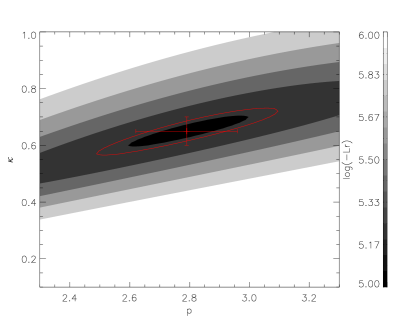
Figure 3: Reduced likelihood surface of the halo parameters $p$ and $\kappa$ space (see Table 2). The best-fitted values and uncertainties are marked as a red plus with error bars. The red contour ellipse shows the likelihood ranges used for estimating the uncertainties.

Table 3: The best-fit values of the disk fit

Bin	$n_{1}$	$L_{1}$	$H_{1}$	$f_{2}$	$L_{2}$	$H_{2}$	$f_{H}$	$Lr$
	$10^{-3}$stars $pc^{-3}$	pc	pc	per cent	pc	pc	per cent
Joint fit
$0.5\leq(g-i)_{0}<0.6$	1.25	2343	322	11	3638	794	0.16	$-$86769
$0.6\leq(g-i)_{0}<0.7$	1.20
$1.5\leq(g-i)_{0}<1.6$	0.54
Individual fit
$0.5\leq(g-i)_{0}<0.6$	1.31	1737	321	14	3581	731	0.16	$-$43699
$0.6\leq(g-i)_{0}<0.7$	1.65	2350	284	7	3699	798	0.12	$-$35774
$1.5\leq(g-i)_{0}<1.6$	0.41	2780	359	8	2926	1014	0.50	$-$4028
stddev		429	31	3	360	124	0.02

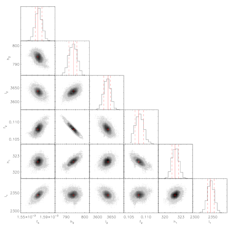
Figure 4: Two-dimensional marginalized PDFs for the disk model parameters, $L_{1},~{}H_{1},~{}f_{2},~{}L_{2},$ and $H_{2}$ and the halo-to-thin disk normalization $f_{h}$, obtained from the MCMC analysis. Histograms on top of each column show the one-dimensional marginalized PDFs of each parameter labeled at the bottom of the column. Red pluses and lines indicate the best solutions. The dash lines give the 16th and 84th percentiles, which denotes only the fitting uncertainties.

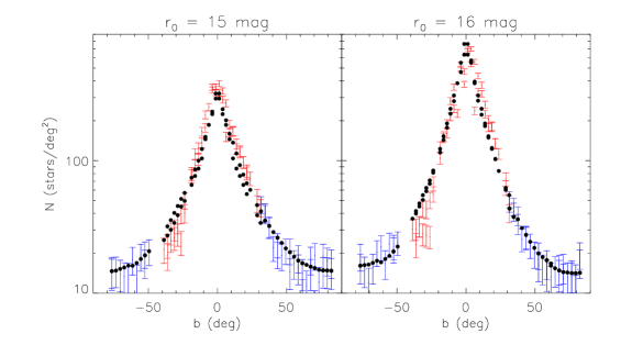
Figure 5: Star count (per deg²) for the colour bin $0.5\leq(g-i)_{0}<0.6$ mag and magnitude bins, $r_{0}$ = 15 (left) and 16 mag (right), of both the XSTPS-GAC (red pluses) and the SDSS (blue pluses) data as a function of the Galactic latitude for example subfields with Galactic longitude 177°$<l<$ 183°. The black dots are the model predictions.

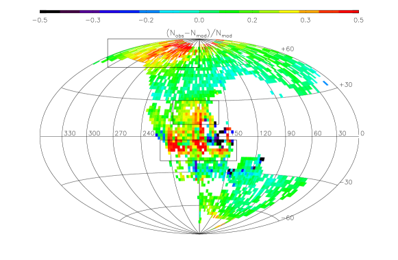
Figure 6: Difference map for the all subfields $(N_{\rm obs}-N_{\rm mod})/N_{\rm mod}$. The populations in excess in the data are most likely irregular structures of the Milky Way. The squares denote different regions with significant excesses of the star counts.

4.1 Fitting results

The best-fit halo model parameters obtained from the halo fit are listed in Table 2 and the reduced likelihood $L_{r}$ surface for the fit is shown in Fig. 3. The $L_{r}$ contour dramatically changes along $\kappa$, but relatively mildly along $p$. The best-fit halo model parameters are $\kappa=0.65\pm 0.05$ and $p=2.79\pm 0.17$. They are not surprisingly in good agreement with those values from Jurić et al. (2008), which have $\kappa=0.64$ and $p=2.8$, since the data used for the halo fit in the current work are mainly from the SDSS subfields. In addition, the photometric parallax relation that Jurić et al. (2008) used for the blue stars was corrected for low-metallicities ([Fe/H] $\sim$ $-$1.5 dex), which is of minor difference from the photometric parallax we used for the halo stars.

The best-fit values for the disk fit are listed in Table 3. We performed the disk fit using first jointly all three colour bins, then separately for each colour bin. For the joint fit case, all the model parameters, excepted for the local density ($n_{0}$), are settled to be the same for stars in every bin, as we expect a universal density profile for all stellar populations (Jurić et al., 2008). All the parameters resulted from the joint fit appear to be very well constrained. We explore the correlations between different parameter pairs in Fig. 4. The Figure shows the marginalized one- and two-dimensional PDFs of the model parameters. The correlations between different parameters are rather weak in general. We identify small correlations between several pairs of the parameters, such as ($H_{1}$, $H_{2}$), ($H_{1}$, $f_{2}$) and ($l_{1}$, $f_{h}$), and a strong degeneracy between the scale height and the local normalised densities ratio of thick disk ($H_{2}$, $f_{2}$).

For the separate fits, we fit all parameters independently for each color bin. The individual fits can be served as a consistency check of our method. From Table 3, we can declare that those best-fit solutions are generally consistent. The thin disk scale height varies around $H_{1}~{}\sim$ 320 pc, by $\pm 40$ pc, which is consistent with the result from the joint fit. The variations of the disk scale lengths are relatively large, with $L_{1}~{}\sim$ 1.7 $-$ 2.8 kpc and $L_{2}~{}\sim$ 2.9 – 3.7 kpc for the thin disk and the thick disk, respectively. The large variations could be due to the limited ranges of Galactocentric distances on the Galactic plane for stars from both the XSTPS-GAC (for the limited depth) and the SDSS (for the poor sky coverage in low Galactic latitudes). Data with deeper depth and better sky coverage in the low Galactic latitudes (such as Pan-Starrs) may help to improve the situation. The thick disk normalization $f_{2}$ and scale height $H_{2}$ appear also weakly constrained, with $f_{2}$ ranging from 7 to 14 per cent and $H_{2}$ from 730 to 1000 pc. This is mainly due to the strong correlation between these two parameters (see the $f_{2}$ vs. $H_{2}$ panel in Fig. 4). The halo normalisation $f_{h}$ is well constrained to $\sim$ 0.15 per cent for the two G-type star bins. While the value of $f_{h}$ is abnormally large for the late K-type star bin [1.5$\leq(g-i)_{0}<$1.6]. This is mainly due to the fact that late K dwarfs in the halo are cut by our limiting magnitude ($r_{0}<$21 mag).

We plot in Fig. 5 the star counts in the colour bin $0.5\leq(g-i)_{0}<0.6$ mag and magnitude bins, $r_{0}=$15 and 16 mag of both the XSTPS-GAC and the SDSS data as a function of the Galactic latitude for example subfields with Galactic longitude 177°$<l<$ 183°. The best-fit model is in good agreement with the observations, with some small deviations. In Fig. 6, we show the differences between the observed star counts, integrated from stars in all the three colour bins and $r_{0}$ from 12 to 21 mag, and the model predictions as a function of position on the sky. Different colours in the Figure indicate the values of the ratio $(N_{\rm obs}-N_{\rm mod})/N_{\rm mod}$. For most of the fields, we do not see obvious deviation, with residual smaller than 10 per cent, i.e. $|(N_{\rm obs}-N_{\rm mod})/N_{\rm mod}|<0.1$.

4.2 Systematics

The dispersions of the resultant parameters from both the jointly fit and individual fit are also listed in Table. 3, which could be used to denote the systematic errors of the corresponding parameters. The typical errors of the parameters are about 10 per cent. Some of the parameters, i.e. the thin disk scale length $H_{1}$ and the thick disk local normalised densities ratio $f_{2}$, have relatively larger uncertainties, which are mainly due to the limits of our data and the degeneracies between different parameters. Other dominant sources of the errors are (in order of decreasing importance): 1) the systematic distance determination uncertainties, 2) the misidentification of binaries as single stars, 3) the value of distance error, i.e., finite width of the photometric parallax relation, 4) the contamination of non-dwarf stars, and 5) the effects from disk warp and flare. Finally, the structure parameters for different stellar populations (colour bins) would be intrinsically different, which may also contribute to the dispersions.

Due to the absolute calibration errors of the photometric parallax relation, the distances of stars could be systematically over- or under- estimated. To check this effects, we redo the fit by changing the distance scale by 􏰎15 per cent, i.e., using the parallax relations 0.3 mag brighter and 0.3 mag fainter than Equation (5). The relative differences between the original resultant parameters and those derived after changing the distance scale by 15 per cent are about 10 – 15 per cent.

Comparing to the single stars of the same colour, the binaries are brighter, i.e. of smaller absolute magnitudes. Thus if one model the Galaxy with no or less fraction of binaries, the resultant model would be more ‘compact’ than it truly is. In the current work we select a binary fraction $f_{b}$=40 per cent, which is an average binary fraction for field FGK stars (Yuan et al., 2015a). To check the possible effects of the binary fraction, we have tried two extreme values, the lowest value, $f_{b}$=0, assuming that all stars are single stars and the highest value, $f_{b}$=1, assuming that all stars are binaries, to redo the fit. The relative differences between the original resultant parameters and those derived after changing the binary fraction to the extreme values are about 10 per cent.

When simulating the star counts for each colour bin, we assumed an error of distances of 15 per cent, which includes the effect of photometric uncertainties, dispersion of metallicities of disk stars and uncertainties of the Ivezić et al. (2008) photometric parallax relation. We redo the fit by changing the distance dispersion to 0 and 30 per cent, respectively. The results show that changing the uncertainties of distance do not introduce any significant bias in the derived Galactic model parameters.

The effects for the model parameters caused by the non-dwarf (i.e. subgiants and giants) contaminations are similar as the binaries. From the Galaxy stellar population synthesis models, BESANCON (Robin et al., 2003) and TRILEGAL (Girardi et al., 2005), we find that the fraction of giants in the three chosen colour bins is no more than 1 per cent and the fraction of sub-giants is less than 5 per cent. Thus the systematics caused by the giant and sub-giant contaminations are likely to be negligible.

In the current work we have ignored the effects of disk flare, as we assume that the stellar flare is becoming significant at further distances (López-Corredoira & Molgó, 2014). While Derriere & Robin (2001) and Amores et al. (2016, submitted) find that the flare starts at about 9 to 10 kpc. Having a shorter start of the flare could have an impact on the thin ansd thick disk scale lengths that we determine, which would make the values to be underestimated.

4.3 Comparisons with other work

As stated in Section 4.1, our results of the halo model parameters are very similar as those derived from Jurić et al. (2008), because of the similar method (stellar number density fits) and data (the SDSS) adopted in both work. The main differences in the halo fit between those from Jurić et al. (2008) and our work are that they adopt the $\chi^{2}$ fitting while we use the reduced likelihood $L_{r}$; and they calculate the number densities for the entire sample in $(R,~{}Z)$ space while we do that separately for each line of sight. The result in our work confirms those from Jurić et al. (2008).

When constraining the disk model parameters, our method and data are both quite different from those in Jurić et al. (2008) but the results are in agreement at a level of about 10 per cent. However, Jurić et al. (2008) admit that their result suffers large uncertainties from the uncertainty in calibration of the photometric parallax relation and the poor sky coverages for the low Galactic latitudes, which is not the case in our work. Generally, our derived value of thin disk scale height, 322 pc, is in the range of values, 150–360 pc, which resulted from the recent work by Bilir et al. (2008); Jurić et al. (2008); Yaz & Karaali (2010); Chang et al. (2011); Polido et al. (2013); Jia et al. (2014) and López-Corredoira & Molgó (2014). Specially, this value is in good agreement with the canonical value of 325 pc (Gilmore, 1984; Yoshii et al., 1987; Reid & Majewski, 1993; Larsen, 1996). Our derived value of the thin disk scale length, 2.3 kpc, is consistent with those results found by Ojha et al. (1996); Robin et al. (2000); Chen et al. (2001); Siegel et al. (2002); Karaali et al. (2007); Jurić et al. (2008); Robin et al. (2012); Polido et al. (2013); López-Corredoira & Molgó (2014) and Yaz Gökçe et al. (2015), which ranges between 2 and 3 kpc. We find a local thick disk normalization of 11 per cent. In the different colour bins, this value varies between 7 and 14 per cent, probably because of the degeneracy with the scale height. It is well in agreement with the values in the literature, which ranges between 7 and 13 per cent (Chen et al., 2001; Siegel et al., 2002; Cabrera-Lavers et al., 2005; Jurić et al., 2008; Chang et al., 2011; Jia et al., 2014). The range of values for the thick disk scale height and scale length from the recent literature are respectively 600 – 1000 pc and 3 – 5 kpc (Bilir et al., 2008; Jurić et al., 2008; Yaz & Karaali, 2010; Chang et al., 2011; Polido et al., 2013; Jia et al., 2014; López-Corredoira & Molgó, 2014; Robin et al., 2014). The results deduced here, which have thick disk scale height of $\sim$800 pc and scale length of 3.6 kpc, are both in the middle of the ranges of those values reported in the literature. Notice that there is a significant difference with the Robin et al. (2014) result for the thick disc. Their thick disk is modelled with 2 episodes, one of which has very similar parameters as the present result (their old thick disk). But their young thick disk is more compact, with smaller scale height and scale length. The difference can be due to the different shapes used (they use secant squared density laws and they include the flare) while in the present study the thick disk is a simple exponential vertically.

5 Substructures

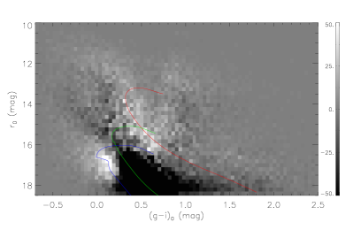
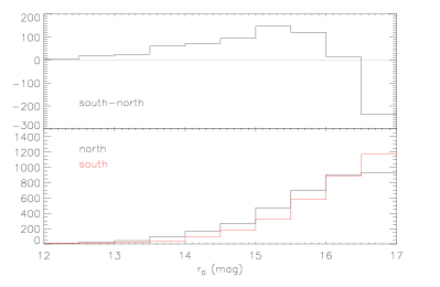
Figure 7: Upper panel: Differences of star counts in the $r_{0}$ vs. $(g-i)_{0}$ diagram for XSTPS-GAC data in 2.5°$\times$ 2.5°patches of sky, i.e. ($l,b$) = (181.25°, $-$8.75°) minus ($l,b$) = (181.25°, 8.75°). The red curve which fits the white main-sequence pattern of the newly identified substructure is an isochrone with [Fe/H]=$-$0.2 dex, age of 3.981 Gyr and distance of 1.3 kpc. The green curve that fits the black main-sequence pattern of the “north near structure” is an isochrone with [Fe/H]=$-$0.5 dex, age of 2.818 Gyr and distance of 3.7 kpc. The blue curve that fits the white main-sequence pattern of the “south middle structure” is an isochrone with [Fe/H]=$-$0.5 dex, age of 1.995 Gyr and distance of 6.8 kpc. Bottom panels: The $r$-band star counts in the colour bin $0.5<(g-i)_{0}<0.6$ mag for the south patch ($l,b$) = (181.25°, $-$8.75°), north patch ($l,b$) = (181.25°, 8.75°) and the subtraction of the two.

One of the main purposes of the Galactic smooth structure modelling is to define the irregular structure of the Milky Way. Assuming that our model now reproduces the populations of the halo and the disk, we can investigate if any further structures are missing from our modelling. As seen in Fig. 6, most of the significant deviations are overdensities, i.e. $N_{obs}>N_{mod}$, except for a few subfields such as those located at ($l,b$)=(170°, 0°). The extinction in these fields are large (Chen et al., 2014). It is very difficult to distinguish that whether it is a real ‘hole’ or it is caused by the selection effects or extinction correction errors. For the overdensities, we find three large scale structures, which are located at different positions on the sky and appear at different magnitudes. We describe them as follows.

The first large region where star counts are in excess is located at 240° $<l<$ 330° and 60° $<b<$ 90°. It is a large and diffuse structure, which corresponds to the Virgo overdensity found by Jurić et al. (2008). For stars with $0.5~{}<~{}(g-i)_{0}~{}<~{}0.7$ mag, the excess of star counts occurs at $r_{0}\sim$20 mag. So the distance of the structure is between 9 – 11 kpc, which is consistent with the work of Jurić et al. (2008). A plausible explanation of the Virgo overdensity is that it is a result of a merger event involving the Milky Way and a smaller, low metallicity dwarf galaxy (Jurić et al., 2008).

The second significant structure is located at 170° $<l<$ 200° and 10°  $<b<$ 30°. The excess of star counts occurs at $r_{0}~{}\sim$ 16 mag for stars with colour $0.5~{}<~{}(g-i)_{0}~{}<~{}0.7$ mag, corresponding to a distance between 1.5–2 kpc. This feature is consistent with the so-called “north near structure” found by Xu et al. (2015). Jurić et al. (2008) also report an overdensity at $R$ = 􏰉 9.5 kpc and $Z$ =􏰉 0.8 kpc, which may be connected with this substructure. Xu et al. (2015) report that this substructure represents one of the locations of peaks in the oscillations of the disk mid-plane, observed at about $\pm$15°Galactic latitude, toward the Galactic anticentre.

The third star counts excess structure is located at 150° $<l<$ 210° and $-$15°  $<b<$ $-5$°. We have not found any corresponding substructures to this feature from the literature. We need to check first that whether this substructure is real or caused by the selection bias or high extinction effects. To test its existence in a more direct way, we examine the Hess diagrams constructed for a subfield located in the area of the feature and for a control subfield which is outside the region. We choose the control subfield with the same galactic longitude but opposite latitude as the selected subfield that includes the overdensity. To avoid the effect of the selection bias of Sample C, we select data from the complete XSTPS-GAC photometric sample in the regions ($l,b$) = (181.25°, $-$8.75°, south field) and (181.25°, 8.75°, north field). Each region is of size 2.5°$\times$ 2.5°. We correct the extinction of stars using the extinction map from Chen et al. (2015) together with the extinction law from Yuan et al. (2013). The average extinction for the south and north fields are respectively $A_{r}$ = 0.66 and 0.27 mag. In Fig. 7, we show the differences between Hess diagrams and the star counts for stars with colour 0.5 $<(g-i)_{0}<$ 0.6 mag for the two regions. We see a white-black-white main-sequence pattern in the difference Hess diagram. The fainter white sequence which indicating that there are more stars on the south side and the middle black sequence indicating that there are more stars on the north side respectively correspond to the “south middle structure” and “north near structure” described in Xu et al. (2015). The bright white sequence corresponds to the newly found substructure. The $r$-band extinction in the these two fields are rather small. Even if we assume an error of 20 per cent in extinction, the uncertainties of colour $g-i$ and magnitude $r$ in the two fields are only $\delta_{g-i}$ = 0.09 and $\delta_{r}$ = 0.13 for the south field and $\delta_{g-i}$ = 0.04 and $\delta_{r}$ = 0.05 for the north field, respectively. The observed feature will not be erased by adjusting the reddening values. So we believe that the feature is real. The effect of selection function and inaccuracies in the reddening correction cannot cause the apparent overdensities.

The excess of star counts occurs at around $r_{0}~{}\sim 15$ mag for stars in the colour ranges of 0.5 $<(g-i)_{0}<$ 0.6 mag, indicating a distance between 1 – 1.5 kpc. We select a series of isochrones from An et al. (2009). The isochrone with [Fe/H] = $-$0.2 dex and age of 3.981 Gyr, shifted by a distance of 1.3 kpc, fit well with the maximum overdensities of the bright white sequence (see Fig. 7 ). The young age and high metallicity are consistent with those of the field thin disk stars. Thus we believe that this feature is unlikely a substructure originated from the outer disk. The distance to the Galactic plane of this feature is about $Z~{}\sim~{}-$0.3 kpc and that for the “north near structure” is about $Z~{}\sim~{}$0.5 kpc. These two features, which show the significant North-South asymmetry in the star number count distributions, are consistent with the vertical oscillations in the stellar density in the solar neighbourhood discovered by Yanny & Gardner (2013, see their Fig. 18).

6 Summary

Based on the data from the XSTPS-GAC and the SDSS, we have modelled the global smooth structure of the Milky Way. We adopt a three-component stellar distribution model. It comprises two double exponential disks, the thin disk and the thick disk, and a two-axial power-law ellipsoid halo. The stellar number density of halo stars in the colour bin $0.5<(g-i)_{0}<0.6$ mag and the $r$-band differential star counts in three colour bins, $0.5<(g-i)_{0}<0.6$ mag, $0.6<(g-i)_{0}<0.7$ mag and $1.5<(g-i)_{0}<1.6$ mag, are used to determine the Galactic model parameters. The best-fit values are listed in Table 2 and 3. In summary, the scale height and length of the thin disk are $H_{1}$=322 pc and $L_{1}$=2343 pc, and those of the thick disk are $H_{2}$=794 pc and $L_{2}$=3638 pc. The local stellar density ratio of thick-to-thin disk is $f_{2}$=11 per cent, and that of halo-to-thin disk is $f_{h}$=0.16 per cent. The axis ratio and power-law index of the halo are $\kappa=0.65$ and $p=2.79$. Our results are all well constrained and in good agreement with the previous works.

By subtracting the observations from our best-fit model, we find three large overdensities. Two of them have been previously identified, including the Virgo overdensity in the Halo (Jurić et al., 2008), which located at 240°  $<l<$ 330° and 60°  $<b<$ 90° with a distance between 9 – 11 kpc, and the so-called “north near structure” in the disk (Xu et al., 2015), which located at 170° $<l<$ 200° and 10° $<b<$ 30° with a distance between 1.5 – 2 kpc. The third structure, located at 150°  $<l<$ 210° and $-$15°  $<b<$ $-5$° with a distance between 1 – 1.5 kpc, is a new identification. Through the Hess diagram examination, we conclude that it could not be a artifact caused by extinction correction or selection effects. This feature, together with the “north near structure” confirms the earlier discovery of Widrow et al. (2012) and Yanny & Gardner (2013) of a significant Galactic North-South asymmetry in the stellar number density distribution.

References

- Abazajian et al. (2004) Abazajian, K., et al. 2004, AJ, 128, 502
- Ak et al. (2007) Ak, S., Bilir, S., Karaali, S., & Buser, R. 2007, Astronomische Nachrichten, 328, 169
- Alam et al. (2015) Alam, S., et al. 2015, ApJS, 219, 12
- Alves (2000) Alves, D. R. 2000, ApJ, 539, 732
- An et al. (2009) An, D., et al. 2009, ApJ, 700, 523
- Bahcall & Soneira (1980) Bahcall, J. N. & Soneira, R. M. 1980, ApJ, 238, L17
- Bienayme et al. (1987) Bienayme, O., Robin, A. C., & Crézé, M. 1987, A&A, 180, 94
- Bilir et al. (2008) Bilir, S., Cabrera-Lavers, A., Karaali, S., Ak, S., Yaz, E., & López-Corredoira, M. 2008, PASA, 25, 69
- Bilir et al. (2006a) Bilir, S., Karaali, S., Ak, S., Yaz, E., & Hamzaoğlu, E. 2006a, New A., 12, 234
- Bilir et al. (2006b) Bilir, S., Karaali, S., Güver, T., Karataş, Y., & Ak, S. G. 2006b, Astronomische Nachrichten, 327, 72
- Bland-Hawthorn & Gerhard (2016) Bland-Hawthorn, J. & Gerhard, O. 2016, ArXiv e-prints
- Bovy et al. (2012) Bovy, J., Rix, H.-W., Liu, C., Hogg, D. W., Beers, T. C., & Lee, Y. S. 2012, The Astrophysical Journal, 753, 148
- Cabrera-Lavers et al. (2007) Cabrera-Lavers, A., Bilir, S., Ak, S., Yaz, E., & López-Corredoira, M. 2007, A&A, 464, 565
- Cabrera-Lavers et al. (2005) Cabrera-Lavers, A., Garzón, F., & Hammersley, P. L. 2005, A&A, 433, 173
- Cabrera-Lavers et al. (2008) Cabrera-Lavers, A., González-Fernández, C., Garzón, F., Hammersley, P. L., & López-Corredoira, M. 2008, A&A, 491, 781
- Chang et al. (2011) Chang, C.-K., Ko, C.-M., & Peng, T.-H. 2011, ApJ, 740, 34
- Chen et al. (2001) Chen, B., et al. 2001, ApJ, 553, 184
- Chen et al. (2015) Chen, B.-Q., Liu, X.-W., Yuan, H.-B., Huang, Y., & Xiang, M.-S. 2015, MNRAS, 448, 2187
- Chen et al. (2014) Chen, B.-Q., et al. 2014, MNRAS, 443, 1192
- Crane et al. (2003) Crane, J. D., Majewski, S. R., Rocha-Pinto, H. J., Frinchaboy, P. M., Skrutskie, M. F., & Law, D. R. 2003, ApJ, 594, L119
- Crézé & Robin (1983) Crézé, M. & Robin, A. 1983, in IAU Colloq. 76: Nearby Stars and the Stellar Luminosity Function, ed. A. G. D. Philip & A. R. Upgren, Vol. 76, 391
- Derriere & Robin (2001) Derriere, S. & Robin, A. C. 2001, in Astronomical Society of the Pacific Conference Series, Vol. 232, The New Era of Wide Field Astronomy, ed. R. Clowes, A. Adamson, & G. Bromage, 229
- Du et al. (2006) Du, C., Ma, J., Wu, Z., & Zhou, X. 2006, MNRAS, 372, 1304
- Frinchaboy et al. (2004) Frinchaboy, P. M., Majewski, S. R., Crane, J. D., Reid, I. N., Rocha-Pinto, H. J., Phelps, R. L., Patterson, R. J., & Muñoz, R. R. 2004, ApJ, 602, L21
- Gilmore (1984) Gilmore, G. 1984, MNRAS, 207, 223
- Gilmore & Reid (1983) Gilmore, G. & Reid, N. 1983, MNRAS, 202, 1025
- Girardi et al. (2005) Girardi, L., Groenewegen, M. A. T., Hatziminaoglou, E., & da Costa, L. 2005, A&A, 436, 895
- Hammersley et al. (2000) Hammersley, P. L., Garzón, F., Mahoney, T. J., López-Corredoira, M., & Torres, M. A. P. 2000, MNRAS, 317, L45
- Hastings (1970) Hastings, W. 1970, Monte Carlo sampling methods using Markov chains and their application.
- Huang et al. (2015) Huang, Y., et al. 2015, Research in Astronomy and Astrophysics, 15, 1240
- Ibata et al. (2003) Ibata, R. A., Irwin, M. J., Lewis, G. F., Ferguson, A. M. N., & Tanvir, N. 2003, MNRAS, 340, L21
- Ivezić et al. (2008) Ivezić, Ž., et al. 2008, ApJ, 684, 287
- Jia et al. (2014) Jia, Y., et al. 2014, MNRAS, 441, 503
- Jurić et al. (2008) Jurić, M., et al. 2008, ApJ, 673, 864
- Kaiser et al. (2002) Kaiser, N., et al. 2002, in Society of Photo-Optical Instrumentation Engineers (SPIE) Conference Series, Vol. 4836, Survey and Other Telescope Technologies and Discoveries, ed. J. A. Tyson & S. Wolff, 154–164
- Karaali et al. (2004) Karaali, S., Bilir, S., & Hamzaoǧlu, E. 2004, MNRAS, 355, 307
- Karaali et al. (2007) Karaali, S., Bilir, S., Yaz, E., Hamzaoğlu, E., & Buser, R. 2007, PASA, 24, 208
- Larsen (1996) Larsen, J. A. 1996, PhD thesis, PhD Thesis, University of Minnesota, (1996)
- Liu et al. (2014) Liu, X.-W., et al. 2014, in IAU Symposium, Vol. 298, IAU Symposium, ed. S. Feltzing, G. Zhao, N. A. Walton, & P. Whitelock, 310–321
- Liu et al. (2015) Liu, X.-W., Zhao, G., & Hou, J.-L. 2015, Research in Astronomy and Astrophysics, 15, 1089
- López-Corredoira et al. (2002) López-Corredoira, M., Cabrera-Lavers, A., Garzón, F., & Hammersley, P. L. 2002, A&A, 394, 883
- López-Corredoira & Molgó (2014) López-Corredoira, M. & Molgó, J. 2014, A&A, 567, A106
- Majewski et al. (2004) Majewski, S. R., Ostheimer, J. C., Rocha-Pinto, H. J., Patterson, R. J., Guhathakurta, P., & Reitzel, D. 2004, ApJ, 615, 738
- Majewski et al. (2003) Majewski, S. R., Skrutskie, M. F., Weinberg, M. D., & Ostheimer, J. C. 2003, ApJ, 599, 1082
- Metropolis et al. (1953) Metropolis, N., Rosenbluth, A., Rosenbluth, M., Teller, A., & Teller, E. 1953, Equations of state calculations by fast computing machines.
- Momany et al. (2006) Momany, Y., Zaggia, S., Gilmore, G., Piotto, G., Carraro, G., Bedin, L. R., & de Angeli, F. 2006, A&A, 451, 515
- Newberg et al. (2002) Newberg, H. J., et al. 2002, ApJ, 569, 245
- Nishiyama et al. (2005) Nishiyama, S., et al. 2005, ApJ, 621, L105
- Ojha et al. (1996) Ojha, D. K., Bienayme, O., Robin, A. C., Crézé, M., & Mohan, V. 1996, A&A, 311, 456
- Ortiz & Lepine (1993) Ortiz, R. & Lepine, J. R. D. 1993, A&A, 279, 90
- Perryman et al. (2001) Perryman, M. A. C., et al. 2001, A&A, 369, 339
- Polido et al. (2013) Polido, P., Jablonski, F., & Lépine, J. R. D. 2013, ApJ, 778, 32
- Reid & Majewski (1993) Reid, N. & Majewski, S. R. 1993, ApJ, 409, 635
- Reylé et al. (2009) Reylé, C., Marshall, D. J., Robin, A. C., & Schultheis, M. 2009, A&A, 495, 819
- Robin et al. (2012) Robin, A. C., Marshall, D. J., Schultheis, M., & Reylé, C. 2012, A&A, 538, A106
- Robin et al. (2000) Robin, A. C., Reylé, C., & Crézé, M. 2000, A&A, 359, 103
- Robin et al. (2003) Robin, A. C., Reylé, C., Derrière, S., & Picaud, S. 2003, A&A, 409, 523
- Robin et al. (2014) Robin, A. C., Reylé, C., Fliri, J., Czekaj, M., Robert, C. P., & Martins, A. M. M. 2014, A&A, 569, A13
- Rocha-Pinto et al. (2003) Rocha-Pinto, H. J., Majewski, S. R., Skrutskie, M. F., & Crane, J. D. 2003, ApJ, 594, L115
- Rocha-Pinto et al. (2004) Rocha-Pinto, H. J., Majewski, S. R., Skrutskie, M. F., Crane, J. D., & Patterson, R. J. 2004, ApJ, 615, 732
- Schlegel et al. (1998) Schlegel, D. J., Finkbeiner, D. P., & Davis, M. 1998, ApJ, 500, 525
- Sesar et al. (2006) Sesar, B., et al. 2006, AJ, 131, 2801
- Siegel et al. (2002) Siegel, M. H., Majewski, S. R., Reid, I. N., & Thompson, I. B. 2002, ApJ, 578, 151
- Skrutskie et al. (2006) Skrutskie, M. F., et al. 2006, AJ, 131, 1163
- van Loon et al. (2003) van Loon, J. T., et al. 2003, MNRAS, 338, 857
- Widrow et al. (2012) Widrow, L. M., Gardner, S., Yanny, B., Dodelson, S., & Chen, H.-Y. 2012, ApJ, 750, L41
- Wright et al. (2010) Wright, E. L., et al. 2010, AJ, 140, 1868
- Xiang et al. (2015) Xiang, M.-S., et al. 2015, Research in Astronomy and Astrophysics, 15, 1209
- Xu et al. (2015) Xu, Y., Newberg, H. J., Carlin, J. L., Liu, C., Deng, L., Li, J., Schönrich, R., & Yanny, B. 2015, ApJ, 801, 105
- Yanny & Gardner (2013) Yanny, B. & Gardner, S. 2013, ApJ, 777, 91
- Yaz & Karaali (2010) Yaz, E. & Karaali, S. 2010, New A., 15, 234
- Yaz Gökçe et al. (2015) Yaz Gökçe, E., et al. 2015, PASA, 32, e012
- York et al. (2000) York, D. G., et al. 2000, AJ, 120, 1579
- Yoshii et al. (1987) Yoshii, Y., Ishida, K., & Stobie, R. S. 1987, AJ, 93, 323
- Yuan et al. (2015a) Yuan, H., Liu, X., Xiang, M., Huang, Y., Chen, B., Wu, Y., Hou, Y., & Zhang, Y. 2015a, ApJ, 799, 135
- Yuan et al. (2015b) Yuan, H.-B., et al. 2015b, MNRAS, 448, 855
- Yuan et al. (2013) Yuan, H. B., Liu, X. W., & Xiang, M. S. 2013, MNRAS, 430, 2188
- Zhang et al. (2013) Zhang, H.-H., Liu, X.-W., Yuan, H.-B., Zhao, H.-B., Yao, J.-S., Zhang, H.-W., & Xiang, M.-S. 2013, Research in Astronomy and Astrophysics, 13, 490
- Zhang et al. (2014) Zhang, H.-H., Liu, X.-W., Yuan, H.-B., Zhao, H.-B., Yao, J.-S., Zhang, H.-W. Xiang, M.-S., & Huang, Y. 2014, Research in Astronomy and Astrophysics, 14, 456