Any-time Diverse Subgroup Discovery with Monte Carlo Tree Search

Abstract

The discovery of patterns that accurately discriminate one class label from another remains a challenging data mining task. Subgroup discovery (SD) is one of the frameworks that enables to elicit such interesting patterns from labeled data. A question remains fairly open: How to select an accurate heuristic search technique when exhaustive enumeration of the pattern space is infeasible? Existing approaches make use of beam-search, sampling, and genetic algorithms for discovering a pattern set that is non-redundant and of high quality w.r.t. a pattern quality measure. We argue that such approaches produce pattern sets that lack of diversity: Only few patterns of high quality, and different enough, are discovered. Our main contribution is then to formally define pattern mining as a game and to solve it with Monte Carlo tree search (MCTS). It can be seen as an exhaustive search guided by random simulations which can be stopped early (limited budget) by virtue of its best-first search property. We show through a comprehensive set of experiments how MCTS enables the anytime discovery of a diverse pattern set of high quality. It outperforms other approaches when dealing with a large pattern search space and for different quality measures. Thanks to its genericity, our MCTS approach can be used for SD but also for many other pattern mining tasks.

1 Introduction

The discovery of patterns, or descriptions, which discriminate a group of objects given a target (class label) has been widely studied as overviewed by [45]. Discovering such descriptive rules can be formalized as the so-called subgroup discovery task (SD introduced by [55]). Given a set of objects, each being associated to a description and a class label, a subgroup is a description generalization whose discriminating ability is evaluated by a quality measure (F1-score, accuracy, etc). In the last two decades, different aspects of SD have been studied: The description and target languages (itemset, sequences, graphs on one side, quantitative and qualitative targets on the other), the algorithms that enable the discovery of the best subgroups, and the definition of measures that express pattern interestingness. These directions of work are closely related and many of the pioneer approaches were ad hoc solutions lacking from easy implementable generalizations (see for examples the surveys of [45] and [17]). SD still faces two important challenges: First, how to characterize the interest of a pattern? Secondly, how to design an accurate heuristic search technique when exhaustive enumeration of the pattern space is unfeasible?

[38] introduced a more general framework than SD called exceptional model mining (EMM). It tackles the first issue. EMM aims to find patterns that cover tuples that locally induce a model that substantially differs from the model of the whole dataset, this difference being measured with a quality measure. This rich framework extends the classical SD settings to multi-labeled data and it leads to a large class of models, quality measures, and applications [[53, 17, 33]]. In a similar fashion to other pattern mining approaches, SD and EMM have to perform a heuristic search when exhaustive search fails. The most widely used techniques are beam search [[53, 42]], genetic algorithms [[15, 41]], and pattern sampling [[43, 7]].

The main goal of these heuristics is to drive the search towards the most interesting parts, i.e., the regions of the search space where patterns maximize a given quality measure. However, it often happens that the best patterns are redundant: They tend to represent the same description, almost the same set of objects, and consequently slightly differ on their pattern quality measures. Several solutions have been proposed to filter out redundant subgroups, e.g. as did [12, 53, 42, 10]. Basically, a neighboring function enables to keep only local optima. However, one may end up with a pattern set of small cardinality: This is the problem of diversity, that is, many local optima have been missed.

Let us illustrate this problem on Figure 1. The search space of patterns, which can be represented as a lattice, hides several local optima (patterns maximizing a pattern quality measure in a neighborhood). Figure 1(a) presents such optima with red dots, surrounded with redundant patterns in their neighborhood. Given the minimal number of objects a pattern must cover, exhaustive search algorithms, such as SD-Map [[4, 3]], are able to traverse this search space efficiently: The monotonocity of the minimum support and upper bounds on some quality measures such as the weighted relative accuracy ($WRAcc$) enable efficient and safe pruning of the search space. However, when the search space of patterns becomes tremendously large, either the number of patterns explodes or the search is intractable. Figure 1(b) presents beam-search, probably the most popular technique within the SD and EMM recent literature. It operates a top-down level-wise greedy exploration of the patterns with a controlled level width that penalizes diversity (although several enhancements to favor diversity have been devised [[53, 54, 42]]). Genetic algorithms have been proposed as well [[47, 46, 14]]. They give however no guarantees that all local optima will be found and they have been designed for specific pattern languages and quality measures [[41]]. Finally, pattern sampling is attractive as it enables direct interactions with the user for using his/her preferences to drive the search [[9, 43]]. Besides, with sampling methods, a result is available anytime. However, traditional sampling methods used for pattern mining need a given probability distribution over the pattern space which depends on both the data and the measure and may be costly to compute [[9, 43]]. Each iteration is independent and draws a pattern given this probability distribution (Figure 1(c)).

In this article, we propose to support subgroup discovery with a novel search method, Monte Carlo tree search (MCTS). It has been mainly used in AI for domains such as games and planning problems, that can be represented as trees of sequential decisions [[13]]. It has been popularized as definitively successful for the game of Go in [50]. MCTS explores a search space by building a game tree in an incremental and asymmetric manner: The tree construction is driven by random simulations and an exploration/exploitation trade-off provided by the so called upper confidence bounds (UCB) [[35]]. The construction can be stopped anytime, e.g., when a maximal budget is reached. As illustrated on Figure 1(d), our intuition for pattern mining is that MCTS searches for some local optima, and once found, the search can be redirected towards other local optima. This principle enables per se a diversity of the result set: Several high quality patterns covering different parts of the data set can be extracted. More importantly, the power of random search leads to anytime mining: A solution is always available, it improves with time and it converges to the optimal one if given enough time and memory budget. This is a best-first search. Given a reasonable time and memory budget, MCTS quickly drives the search towards a diverse pattern set of high quality. Interestingly, it can consider, in theory, any pattern quality measure and pattern language (in contrast to current sampling techniques as developped by [9, 43]).

Our main contribution is to a complete characterization of MCTS for subgroup discovery and pattern mining in general. Revisiting MCTS in such a setting is not simple and the definition of it requires smart new policies. We show through an extensive set of experiments that MCTS is a compelling solution for a pattern mining task and that it outperforms the state-of-the-art approaches (exhaustive search, beam search, genetic algorithm, pattern sampling) when dealing with large search space of numerical and nominal attributes and for different quality measures.

The rest of this article is organized as follows. Section 2 formally introduces the pattern set discovery problem. Section 3 then recalls the basic definitions of MCTS. We present our MCTS method, called mcts4dm, in Section 4. After discussing the related work in Section 5, we report on experiments for understanding how to configure a MCTS for pattern mining (Section 6) and how does MCTS compare to competitors (Section 7).

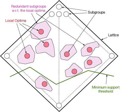
(a) Redundancy problem.

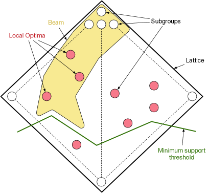
(b) Beam search.

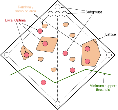
(c) Sampling exploration.

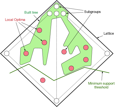
(d) MCTS-based exploration.

Figure 1: Illustration of different SD search algorithms.

2 Pattern set discovery

There exists several formal pattern mining frameworks and we choose here subgroup discovery to illustrate our purpose. We provide some basic definitions and then formally define pattern set discovery.

Definition 1 (Dataset $\mathcal{D}(\mathcal{O},\mathcal{A},\mathcal{C},\mathit{class})$).

Let $\mathcal{O}$, $\mathcal{A}$ and $\mathcal{C}$ be respectively a set of objects, a set of attributes, and a set of class labels. The domain of an attribute $a\in\mathcal{A}$ is $Dom(a)$ where $a$ is either nominal or numerical. The mapping $\mathit{class}:\mathcal{O}\mapsto{\mathcal{C}}$ associates each object to a unique class label.

A subgroup can be represented either by a description (the pattern) or by its coverage, also called its extent.

Table 1: Toy dataset

ID	$a$	$b$	$c$	$\mathit{class}(.)$
1	150	21	11	$l_{1}$
2	128	29	9	$l_{2}$
3	136	24	10	$l_{2}$
4	152	23	11	$l_{3}$
5	151	27	12	$l_{2}$
6	142	27	10	$l_{1}$

Definition 2 (Subgroup).

The description of a subgroup, also called pattern, is given by $d=\langle f_{1},\dots,f_{|\mathcal{A}|}\rangle$ where each $f_{i}$ is a restriction on the value domain of the attribute $a_{i}\in\mathcal{A}$. A restriction for a nominal attribute $a_{i}$ is a symbol $a_{i}=v$ with $v\in Dom(a_{i})$. A restriction for a numerical attribute $a_{i}$ is an interval $[l,r]$ with $l,r\in Dom(a_{i})$. The description $d$ covers a set of objects called the extent of the subgroup, denoted $ext(d)\subseteq\mathcal{O}$. The support of a subgroup is the cardinality of its extent: $supp(d)=|ext(d)|$.

The subgroup search space is structured as a lattice.

Definition 3 (Subgroup search space).

The set of all subgroups forms a lattice, denoted as the poset $(\mathcal{S},\preceq)$. The top is the most general pattern, without restriction. Given any $s_{1},s_{2}\in\mathcal{S}$, we note $s_{1}\prec s_{2}$ to denote that $s_{1}$ is strictly more specific, i.e. it contains more stringent restrictions.

If follows that $ext(s_{1})\subseteq ext(s_{2})$ when $s_{1}\preceq s_{2}$.

The ability of a subgroup to discriminate a class label is evaluated by means of a quality measure. The weighted relative accuracy (WRAcc), intoduced by [37], is among the most popular measures for rule learning and subgroup discovery. Basically, WRAcc considers the precision of the subgroup w.r.t. to a class label relatively to the appearance probability of the label in the whole dataset. This difference is weighted with the support of the subgroup to avoid to consider small ones as interesting.

Definition 4 (WRAcc).

Given a dataset $\mathcal{D}(\mathcal{O},\mathcal{A},\mathcal{C},\mathit{class})$, the WRAcc of a subgroup $d$ for a label $l\in Dom(\mathcal{C})$ is given by:

$$\textit{WRAcc}(d,l)=\frac{supp(d)}{|\mathcal{O}|}\times\left(p^{l}_{d}-p^{l}\right)$$

where ${p^{l}_{d}=\frac{|\{o\in ext(d)|class(o)=l\}|}{supp(d)}}$ and ${p^{l}=\frac{|\{o\in\mathcal{O}|class(o)=l\}|}{|\mathcal{O}|}}$.

WRAcc returns values in $[-0.25,0,25]$, the higher and positive, the better the pattern discriminates the class label. Many quality measures other than WRAcc have been introduced in the literature of rule learning and subgroup discovery (Gini index, entropy, F score, Jaccard coefficient, etc. [[2]]). Exceptional model mining (EMM) considers multiple labels (label distribution difference in [53], Bayesian model difference in [19], etc.). The choice of a pattern quality measure, denoted $\varphi$ in what follows, is generally application dependant as explained by [22].

Example 1.

Consider the dataset in Table 1 with objects in $\mathcal{O}=\{1,...,6\}$ and attributes in $\mathcal{A}=\{a,b,c\}$. Each object is labeled with a class label from $\mathcal{C}=\{l_{1},l_{2},l_{3}\}$. Consider an arbitrary subgroup with description $d=\langle[128\leq a\leq 151],[23\leq b\leq 29]\rangle$. Note that, for readability, we omit restrictions satisfied by all objects, e.g., $[9\leq c\leq 12]$, and thus we denote that $ext(\langle\rangle)=\mathcal{O}$. The extent of $d$ is composed of the objects in $ext(d)=\{2,3,5,6\}$ and we have ${WRAcc(d,l_{2})=\frac{4}{6}(\frac{3}{4}-\frac{1}{2})=\frac{1}{6}}$. The upper part of the search space (most general subgroups) is given in Figure 2. The direct specializations of a subgroup are given, for each attribute, by adding a restriction: Either by shrinking the interval of values to the left (take the right next value in its domain) or to the right (take the left next value). In this way, the finite set of all intervals taking borders in the attributes domain will be explored (see [32]).

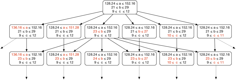
Figure 2: The upper part of the search space for Table 1.

Pattern set discovery consists in searching for a set of patterns $\mathcal{R}\subseteq\mathcal{S}$ of high quality on the quality measure $\varphi$ and whose patterns are not redundant. As similar patterns generally have similar values on $\varphi$, we design the pattern set discovery problem as the identification of the local optima w.r.t. $\varphi$. As explained below, this has two main advantages: Redundant patterns of lower quality on $\varphi$ are pruned and the extracted local optima are diverse and potentially interesting patterns.

Definition 5 (Local optimum as a non redundant pattern).

Let $sim:\mathcal{S}\times\mathcal{S}\rightarrow[0,1]$ be a similarity measure on $\mathcal{S}$ that, given a real value $\Theta>0$, defines neighborhoods on $\mathcal{R}\subseteq\mathcal{S}:N_{\mathcal{R}}(x)=\{s\in\mathcal{R}\mid sim(x,s)\geq\Theta\}$. $r^{\star}$ is a local optimum of $\mathcal{R}$ on $\varphi$ iff $\forall r\in N_{\mathcal{R}}(r^{\star})$, $\varphi(r^{\star})\geq\varphi(r)$. We denote by $filter(\mathcal{R})$ the set of local optima of $\mathcal{R}$ and by $redundancy(\mathcal{R})=1-\frac{|filter(\mathcal{R})|}{|\mathcal{R}|}$ the measure of redundancy of $\mathcal{R}$.

In this paper, the similarity measure on $\mathcal{S}$ will be the Jaccard measure defined by

$$sim(r,r^{\prime})=\frac{ext(r)\cap ext(r^{\prime})}{ext(r)\cup ext(r^{\prime})}$$

We propose to evaluate the diversity of a pattern set $\mathcal{R}\subseteq\mathcal{S}$ by the sum of the quality of its patterns. Indeed, the objective is to obtain the largest set of high quality patterns:

Definition 6 (Pattern set diversity).

The diversity of a pattern set $\mathcal{R}$ is evaluated by: $diversity(\mathcal{R})=\sum_{r\in filter(\mathcal{R})}\varphi(r)$.

The function $filter()$ is generally defined in a greedy or heuristic way in the literature. [53] called it pattern set selection and we use their implementation in this article. First all extracted patterns are sorted according to the quality measure and the best one is kept. The next patterns in the order are discarded if they are too similar with the best pattern (Jaccard similarity between pattern supports is used). Once a non similar pattern is found, it is kept for the final result and the process is reiterated: Following patterns will be compared to it.

Problem 1 (Pattern set discovery).

Compute a set of patterns $\mathcal{R}^{*}\subseteq\mathcal{S}$ such that $\forall r\in\mathcal{R}^{*}$, $r$ is a local optimum on $\varphi$ and

$$\mathcal{R}^{*}=\mbox{argmax}_{\mathcal{R}\subseteq\mathcal{S}}diversity(\mathcal{R}).$$

By construction, $\mathcal{R}^{*}$ maximizes diversity and it minimizes redundancy. Naturally, $\mathcal{R}^{*}$ is not unique. Existing approaches sometimes search for a pattern set of size $k$ [[41]], with a minimum support threshold $minSupp$ [[4]].

3 Monte Carlo tree search

MCTS is a search method used in several domains to find an optimal decision (see the survey by [13]). It merges theoretical results from decision theory [[48]], game theory, Monte Carlo [[1]] and bandit-based methods [[5]]. MCTS is a powerful search method because it enables the use of random simulations for characterizing a trade-off between the exploration of the search tree and the exploitation of an interesting solution, based on past observations. Considering a two-players game (e.g., Go): The goal of MCTS is to find the best action to play given a current game state. MCTS proceeds in several (limited) iterations that build a partial game tree (called the search tree) depending on the results of previous iterations. The nodes represent game states. The root node is the current game state. The children of a node are the game states accessible from this node by playing an available action. The leaves are the terminal game states (game win/loss/tie). Each iteration, consisting of 4 steps (see Figure 3), leads to the generation of a new node in the search tree (depending on the exploration/exploitation trade-off due to the past iterations) followed by a simulation (sequence of actions up to a terminal node). Any node $s$ in the search tree is provided with two values: The number $N(s)$ of times it has been visited, and a value $Q(s)$ that corresponds to the aggregation of rewards of all simulations walked through $s$ so far (e.g., the proportion of wins obtained for all simulations walked through $s$). The aggregated reward of each node is updated through the iterations such that it becomes more and more accurate. Once the computation budget is reached, MCTS returns the best move that leads to the child of the root node with the best aggregated reward $Q(.)$.

In the following, we detail the 4 steps of a MCTS iteration applied to a game. Algorithm 3.1 gives the pseudo code of the most popular algorithm in the MCTS family, namely UCT (upper confidence bound for trees), as given in [35].

Algorithm 3.1.

1:function Mcts($\mathit{budget}$)

2:     create root node $s_{0}$ for current state

3:     while within computational budget $\mathit{budget}$ do

4:         $s_{sel}\leftarrow$ Select($s_{0}$)

5:         $s_{exp}\leftarrow$ Expand($s_{sel}$)

6:         $\Delta\leftarrow$ RollOut($s_{exp}$)

7:         Update($s_{exp},\Delta$)

8:     end while

9:     return the action that reaches the child $s$ of $s_{0}$ with the highest $Q(s)$

10:end function

11:

12:function Select($s$)

13:     while $s$ is non-terminal do

14:         if $s$ is not fully expanded then   return $s$

15:         else  $s\leftarrow$ BestChild($s$)

16:         end if

17:     end while

18:     return $s$

19:end function

20:

21:function Expand($s_{sel}$)

22:     randomly choose $s_{exp}$ from non expanded children of $s_{sel}$

23:     add new child $s_{exp}$ to $s_{sel}$

24:     return $s_{exp}$

25:end function

26:

27:function RollOut($s$)

28:     $\Delta\leftarrow 0$

29:     while $s$ is non-terminal do

30:         choose randomly a child $s^{\prime}$ of $s$

31:         $s\leftarrow s^{\prime}$

32:     end while

33:     return the reward of the terminal state $s$

34:end function

35:

36:function Update($s,\Delta$)

37:     while $s$ is not null do

38:         $Q(s)\leftarrow\frac{N(s)\times Q(s)+\Delta}{N(s)+1}$

39:         $N(s)\leftarrow N(s)+1$

40:         $s\leftarrow$ parent of $s$

41:     end while

42:end function

43:

44:function BestChild($s$)

45:     return $\operatorname*{arg\,max}\limits_{s^{\prime}\in\ children\ of\ s}UCB(s,s^{\prime})$

46:end function

UCT: The popular MCTS algorithm.

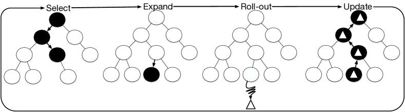
Figure 3: One MCTS iteration (taken from [13]).

The Select policy. Starting from the root node, the Select method recursively selects an action (an edge) until the selected node is either a terminal game state or is not fully expanded (i.e., some children of this node are not yet expanded in the search tree). The selection of a child of a node $s$ is based on the exploration/exploitation trade-off. For that, upper confidence bounds (UCB) are used. They bound the regret of choosing a non-optimal child. The original UCBs used in MCTS are the UCB1 from [5] and the UCT from [35]:

$$UCT(s,s^{\prime})=Q(s^{\prime})+2C_{p}\sqrt{\frac{2\ln N(s)}{N(s^{\prime})}}$$

where $s^{\prime}$ is a child of a node $s$ and $C_{p}>0$ is a constant (generally, $C_{p}=\frac{1}{\sqrt{2}}$). This step selects the most urgent node to be expanded, called $s_{sel}$ in the following, considering both the exploitation of interesting actions (given by the first term in UCT) and the exploration of lightly explored areas of the search space (given by the second term in UCT) based on the result of past iterations. The constant $C_{p}$ can be adjusted to lower or increase the exploration weight in the exploration/exploitation trade-off . Note that when $C_{p}=\frac{1}{2}$, the UCT is called UCB1.

The Expand policy. A new child, denoted $s_{exp}$, of the selected node $s_{sel}$ is added to the tree according to the available actions. The child $s_{exp}$ is randomly picked among all available children of $s_{sel}$ not yet expanded in the search tree.

The RollOut policy. From this expanded node $s_{exp}$, a simulation is played based on a specific policy. This simulation consists of exploring the search tree (playing a sequence of actions) from $s_{exp}$ until a terminal state is reached. It returns the reward $\Delta$ of this terminal state: $\Delta=1$ if the terminal state is a win, $\Delta=0$ otherwise.

The Update policy. The reward $\Delta$ is back-propagated to the root, updating for each parent the number of visits $N(.)$ (incremented by 1) and the aggregation reward $Q(.)$ (the new proportion of wins).

Example. Figure 3 depicts a MCTS iteration. Each node has no more than 2 children. In this scenario, the search tree is already expanded: We consider the $9^{th}$ iteration since $8$ nodes of the tree have been already added. The first step consists in running the Select method starting from the root node. Based on a UCB, the selection policy chooses the left child of the root. As this node is fully expanded, the algorithm randomly selects a new node among the children of this node: Its right child. This selected node $s_{sel}$ is not fully expanded since its left hand side child is not in the search tree yet. From this not fully expanded node $s_{sel}$, the Expand method adds the left hand side child $s_{exp}$ of the selected node $s_{sel}$ to expand the search tree. From this added node $s_{exp}$, a random simulation is rolled out until reaching a terminal state. The reward $\Delta$ of the terminal node is back-propagated with Update.

4 Pattern set discovery with MCTS

Designing a MCTS approach for a pattern mining problem is different than for a combinatorial game: The goal is not to decide, at each turn, what is the best action to play, but to explore the search space: The pattern mining problem can thus be considered as a single-turn single-player game. Most importantly, MCTS offers a natural way to explore the search space of patterns with the benefit of the exploitation/exploration trade-off to improve diversity while limiting redundancy. For example, an exhaustive search will maximize diversity, but it will return a very large and redundant collection (but an exhaustive search is usually impossible). In contrast, a beam search can extract a limited number of patterns but it will certainly lack diversity (empirical evidences are given later in Section 7).

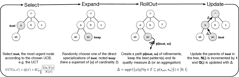
Figure 4: A simple instanciation of MCTS for pattern mining.

Before going into the formalization, let us illustrate how MCTS is applied to the pattern set discovery problem with Figure 4. We consider here itemset patterns for the sake of simplicity, that is, subgroups whose descriptions are sets of items. We present an iteration of a MCTS for a transaction database with items $\mathcal{I}=\{a,b,c\}$. The pattern search space is given by the lattice $\mathcal{S}=(2^{\mathcal{I}},\subseteq)$. The MCTS tree is built in a top-down fashion on this theoretical search space: The initial pattern, or root of the tree, is the empty set $\emptyset$. Assume that pattern $s_{sel}=\{a\}$ has been chosen by the select policy. During the expand, one of its direct specializations in $\{\{a,b\},\{a,c\}\}$ is randomly chosen and added to the tree,e.g., $s_{exp}=\{a,c\}$. During the roll out, a simulation is run from this node: it generates a chain of specializations of $s_{exp}$ called a path $p(s_{sel},s_{n})$ (a chain is a set of comparable patterns w.r.t. $\subseteq$, or $\preceq$ in the general case). The quality measure $\varphi$ is computed for each pattern of the path, and an aggregated value (max, mean, etc.) is returned and called $\Delta$. Finally, all parents of $s_{exp}$ are updated: Their visit count $N(.)$ is incremented by one, while their quality estimation $Q(.)$ is recomputed with $\Delta$ (back propagation). The new values of $N(.)$ and $Q(.)$ will directly impact the selection of the next iteration when computing the chosen UCB, and thus the desired exploration/exploitation trade off. When the budget is exceeded (or if the tree is fully expanded), all patterns are filtered with a chosen pattern set selection strategy ($filter(.)$).

The expected shape of the MCTS tree after a high number of iterations is illustrated in Figure 1d. It suggests a high diversity of the final pattern set if given enough budget (i.e., enough iterations). However, how to properly define each policy (select, expand, roll out and update), is not obvious. Table 2 sums up the different policies that we use or develop specifically for a pattern mining problem.

Select

Choose one of the following UCB:

UCB1 or UCB1-Tuned or SP-MCTS or UCT

Expand

direct-expand: Randomly choose the next direct expansion

gen-expand: Randomly choose the next direct expansion until it changes the extent

label-expand: Randomly choose the next direct expansion until it changes the true positives

Activate LO: Generate each pattern only once (lectic enumeration)

Activate PU: Patterns with the same support/true positive set point to the same node

RollOut

naive-roll-out: Generate a random path of direct specializations of random length.

direct-freq-roll-out: Generate a random path of frequent direct specializations.

large-freq-roll-out: Generate a random paths of undirect specializations (random jumps).

Memory

no-memory: No pattern found during the simulation is kept for the final result.

top-k-memory: Top-k patterns of a simulation are considered in memory.

all-memory: All patterns generated during the simulation are kept.

Update

max-update: Only the maximum $\varphi$ found in a simulation is back propagated

mean-update: The average of all $\varphi$ is back-propagated

top-k-mean-update: The average of the best $k$ $\varphi$ is back-propagated

Table 2: The different policies

4.1 The Select method

The Select method has to select the most promising node $s_{sel}$ in terms of the exploration vs. exploitation trade-off. For that, the well-known bounds like UCT or UCB1 can be used. However, more sophisticated bounds have been designed for single player games. The single-player MCTS (SP-MCTS), introduced by [49], adds a third term to the UCB to take into account the variance $\sigma^{2}$ of the rewards obtained by the child so far. SP-MCTS of a child $s^{\prime}$ of a node $s$ is:

$$\textit{SP-MCTS}(s,s^{\prime})=Q(s^{\prime})+C\sqrt{\frac{2\ln N(s)}{N(s^{\prime})}}+\sqrt{\sigma^{2}(s^{\prime})+\frac{D}{N(s^{\prime})}}$$

where the constant $C$ is used to weight the exploration term (it is fixed to $0.5$ in its original definition) and the term $\frac{D}{N(s^{\prime})}$ inflates the standard deviation for infrequently visited children ($D$ is also a constant). In this way, the reward of a node rarely visited is considered as less certain: It is still required to explore it to get a more precise estimate of its variance. If the variance is still high, it means that the subspace from this node is not homogeneous w.r.t. the quality measure and further exploration is needed.

Also, [5] designed UCB1-Tuned to reduce the impact of the exploration term of the original UCB1 by weighting it with either an approximation of the variance of the rewards obtained so far or the factor $1/4$. UCB1-Tuned of a child $s^{\prime}$ of $s$ is:

$$\textit{UCB1-Tuned}(s,s^{\prime})=Q(s^{\prime})+\sqrt{\frac{\ln N(s)}{N(s^{\prime})}\min{(\frac{1}{4},\sigma^{2}(s^{\prime})+\sqrt{\frac{2\ln{N(s)}}{N(s^{\prime})}})}}$$

The only requirement the pattern quality measure $\varphi$ must satisfy is, in case of UCT only, to take values in $[0,1]$: $\varphi$ can be normalized in this case.

4.2 The Expand method

The Expand step consists in adding a pattern specialization as a new node in the search tree. In the following, we present different refinement operators, and how to avoid duplicate nodes in the search tree.

4.2.1 The refinement operators

A simple way to expand the selected node $s_{sel}$ is to choose uniformly an available attribute w.r.t. $s_{sel}$, that is to specialize $s_{sel}$ into $s_{exp}$ such that $s_{exp}\prec s_{sel}$: $s_{exp}$ is a refinement of $s_{sel}$. It follows that $ext(s_{exp})\subseteq ext(s_{sel})$, and obviously $supp(s_{exp})\leq supp(s_{sel})$, known as the monotonocity property of the support.

Definition 7 (Refinement operator).

A refinement operator is a function $\mathit{ref}:\mathcal{S}\rightarrow 2^{\mathcal{S}}$ that derives from a pattern $s$ a set of more specific patterns $\mathit{ref}(s)$ such that:

• (i) $\forall s^{\prime}\in\mathit{ref}(s),s^{\prime}\prec s$

• (ii)$\forall s^{\prime}_{i},s^{\prime}_{j}\in\mathit{ref}(s),i\neq j,s^{\prime}_{i}\npreceq s^{\prime}_{j},s^{\prime}_{j}\npreceq s^{\prime}_{i}$

In other words, a refinement operator gives to any pattern $s$ a set of its specializations, that are pairwise incomparable (an anti-chain). The refine operation can be implemented in various ways given the kind of patterns we are dealing with. Most importantly, it can return all the direct specializations only to ensure that the exploration will, if given enough budget, explore the whole search space of patterns. Furthermore, it is unnecessary to generate infrequent patterns.

Definition 8 (Direct-refinement operator).

A direct refinement operator is a refinement operator $\mathit{directRef}:\mathcal{S}\rightarrow 2^{\mathcal{S}}$ that derives from a pattern $s$ the set of direct more specific patterns $s^{\prime}$ such that:

• (i) $\forall s^{\prime}\in\mathit{directRef}(s)$, $s^{\prime}\prec s$

• (ii) $\not\exists s^{\prime\prime}\in\mathcal{S}$ s.t. $s^{\prime}\prec s^{\prime\prime}\prec s$

• (iii) For any $s^{\prime}\in\mathit{directRef}(s)$, $s^{\prime}$ is frequent, that is $supp(s^{\prime})\geq minSupp$

The notion of direct refinement is well known in pattern mining. For instance, the only way to refine a nominal (resp. Boolean) attribute is to assign it a value of its domain (resp. the true value). Refining an itemset consists in adding a item, while refining a numerical attribute can be done in two ways: Applying the minimal left change (resp. right change), that is, increasing the lower bound of the interval to the next higher value in its domain (resp. decreasing the upper bound to the next lower) as explained by [32]. We still use the term restriction to denote the operations that create a direct refinement of pattern.

Definition 9 (The direct-expand strategy).

We define the direct-expand strategy as follows: From the selected node $s_{sel}$, we randomly pick a – not yet expanded – node $s_{exp}$ from $directRef(s_{sel})$ and add it in the search tree.

As most quality measures $\varphi$ used in SD and EMM are solely based on the extent of the patterns, considering only one pattern among all those having the same extent is enough. However, with the direct-refinement operator, a large number of tree nodes may have the same extent as their parent. This redundancy may bias the exploration and more iterations will be required. For that, we propose to use the notion of closed patterns and their generators.

Definition 10 (Closed descriptions and their generators).

The equivalence class of a pattern $s$ is given by $[s]=\{s^{\prime}\in\mathcal{S}~{}|~{}ext(s)=ext(s^{\prime})\}$. Each equivalence class has a unique smallest element w.r.t. $\prec$ that is called the closed pattern: $s$ is said to be closed iff $\not\exists s^{\prime}$ such that $s^{\prime}\prec s$ and $ext(s)=ext(s^{\prime})$. The non-closed patterns are called generators.

Definition 11 (Generator-refinement operator).

A generator refinement operator is a refinement operator $\mathit{genRef}:\mathcal{S}\rightarrow 2^{\mathcal{S}}$ that derives from a pattern $s$ the set of more specific patterns $s^{\prime}$ such that, $\forall s^{\prime}\in\mathit{genRef}(s)$:

• (i) $s^{\prime}\not\in[s]$ (different support)

• (ii) $\not\exists s^{\prime\prime}\in\mathcal{S}\backslash\mathit{genRef}(s)$ s.t. $s^{\prime\prime}\not\in[s]$, $s^{\prime\prime}\not\in[s^{\prime}]$, $s^{\prime}\prec s^{\prime\prime}\prec s$ (direct next equivalence class)

• (iii) $s^{\prime}$ is frequent, that is $supp(s^{\prime})\geq minSupp$ (frequent)

Definition 12 (The gen-expand strategy).

To avoid the exploration of patterns with the same extent in a branch of the tree, we define the min-gen-expand strategy as follows: From the selected node $s_{sel}$, we randomly pick a – not yet expanded – refined pattern from $\mathit{genRef}(s_{sel})$, called $s_{exp}$, and add it to the search tree.

Finally, when facing a SD problem whose aim is to characterize a label $l\in\mathcal{C}$ we can adapt the previous refinement operator based on generators on the extents of both the subgroup and the label. As many other measures, the WRAcc seeks to optimize the (weighted relative) precision or accuracy of the subgroup. The accuracy is the ratio of true positives in the extent. We propose thus, for this kind of measures only, the label-expand strategy: Basically, the pattern is refined until the set of true positives in the extent changes. This minor improvement performs very well in practice (see Section 6).

4.2.2 Avoiding duplicates in the search tree

We define several refinement operators to avoid the redundancy within a branch of the tree, i.e., do not expand $s_{sel}$ with a pattern whose extent is the same because the quality measure $\varphi$ will be equal. However, another redundancy issue remains at the tree scale. Indeed, since the pattern search space is a lattice, a pattern can be generated in nodes from different branches of the Monte Carlo tree, that is, with different sequences of refinements, or simply permutations of refinements. As such, it will happen that a part of the search space is sampled several times in different branches of the tree. However, the visit count $N(s)$ of a node $s$ will not count visits of other nodes that denote exactly the same pattern: The UCB is clearly biased. To tackle this aspect, we implement two methods: (i) Using a lectic order or (ii) detecting and unifying the duplicates within the tree. These two solutions can be used for any refinement operator. Note that enabling both these solutions at the same tame is useless since each of them ensures to avoid duplicates within the tree.

Avoiding duplicates in the tree using a lectic order (LO).

Pattern enumeration without duplicates is at the core of constraint-based pattern-mining [[11]]. Avoiding to generate patterns with the same extent is usually based on a total order on the set of attribute restrictions. This poset is written by $(R,\lessdot)$.

Example 2.

For instance, considering itemset patterns, $R=\mathcal{I}$ and a lectic order, usually the lexicographic order, is chosen on $\mathcal{I}$: $a\lessdot b\lessdot c\lessdot d$ for $I=\{a,b,c,d\}$ and $bc\lessdot ad$. Consider that a node $s$ has been generated with a restriction $r_{i}$: we can expand the node only with restrictions $r_{j}$ such that $r_{i}\lessdot r_{j}$. This total order also holds for numerical attributes by considering the minimal changes (see the work of [32] for further details).

We can use this technique to enumerate the lattice with a depth-first search (DFS), which ensures that each element of the search space is visited exactly once. An example is given in Figure 5. However, it induces a strong bias: An MCTS algorithm would sample this tree instead of sampling the pattern search space. In other words, a small restriction w.r.t. $\lessdot$ has much less chances to be picked than a largest one. Going back to the example in Figure 5 (middle), the item $a$ can be drawn only once through a complete DFS; $b$ twice; while $c$ four times (in bold). It follows that patterns on the left hand side of the tree have less chances to be generated, e.g., $prob(\{a,b\})=1/6$ while $prob(\{b,c\})=1/3$. These two itemsets should however have the same chance to be picked as they have the same size. This variability is corrected by weighting the visit counts in the UCT with the normalized exploration rate (see Figure 5 (right)).

Definition 13 (Normalized exploration rate).

Let $\mathcal{S}$ be the set of all possible patterns. The normalized exploration rate of a pattern $s$ is,

$$\rho_{norm}(s)=\frac{V_{total}(s)}{V_{lectic}(s)}=\frac{|\{s^{\prime}|s^{\prime}\preceq s,\forall s^{\prime}\in\mathcal{S}\}|}{|\{s^{\prime}|(s\lessdot s^{\prime}\wedge s^{\prime}\prec s)\vee s=s^{\prime},\forall s^{\prime}\in\mathcal{S}\}|}$$

Given this normalized exploration rate, we can adapt the UCBs when enabling the lectic order. For example, we can define the DFS-UCT of a child $s^{\prime}$ of a pattern $s$ derived from the UCT as follows:

$$\textit{DFS-UCT}(s,s^{\prime})=Q(s^{\prime})+2C_{p}\sqrt{\frac{2\ln\left(N(s)\cdot\rho_{norm}(s)\right)}{N(s^{\prime})\cdot\rho_{norm}(s^{\prime})}}$$

Proposition 4.1 (Normalized exploration rate for itemsets).

For itemsets, let $s_{i}$ be the child of $s$ obtained by playing action $r_{i}$ and $i$ is the rank of $r_{i}$ in $(R,\lessdot)$: $\rho_{norm}(s_{i})=\frac{2^{(|\mathcal{I}|-|s_{i}|)}}{2^{(|\mathcal{I}|-i-1)}}$.

Proof.

Let $V_{lectic}(s_{i})$ be the size of the search space sampled under $s_{i}$ using a lectic enumeration, and $V_{total}(s_{i})$ be the size of the search space without using a lectic enumeration. Noting $V_{total}(s_{i})=2^{(|\mathcal{I}|-|s_{i}|)}$ and $V_{lectic}(s_{i})=2^{(|\mathcal{I}|-i-1)}$ for itemsets, we have $\rho_{norm}(s_{i})=\frac{V_{total}(s_{i})}{V_{lectic}(s_{i})}=\frac{2^{(|\mathcal{I}|-|s_{i}|)}}{2^{(|\mathcal{I}|-i-1)}}$. ∎∎

Proposition 4.2 (Normalized exploration rate for a numerical attribute).

For a single numerical attribute $a$, $\rho_{norm}(.)$ is defined as follows :

• Let $s^{\prime}=\langle\alpha_{i}\leq a\leq\alpha_{j}\rangle$ obtained after a left change: $\rho_{norm}(s^{\prime})=1$.

• Let $s^{\prime}=\langle\alpha_{i}\leq a\leq\alpha_{j}\rangle$ obtained after a right change. Let $n$ be the number of values from $Dom(a)$ in $[\alpha_{i},\alpha_{j}]$: ${\rho_{norm}(s^{\prime})=\frac{n+1}{2}}$.

Proof.

As explained in the proof of (Proposition 4.1), $\rho_{norm}(s)=\frac{V_{total}(s)}{V_{lectic}(s)}$. For a numerical attribute, $V_{total}(s)=n(n+1)/2$, i.e. the number of all sub intervals. If $s$ was obtained after a left change, $V_{lectic}(s)=n(n+1)/2$ as both left and right changes can be applied. If $s$ was obtained after a right change, $V_{lectic}(s)=n$, as only $n$ right changes can be applied. It follows that $\rho_{norm}(s)=\frac{n(n+1)/2}{n(n+1)/2}=1$ if $s$ was obtained from a left change and $\rho_{norm}(s)=\frac{n(n+1)/2}{n}=\frac{n+1}{2}$ otherwise. ∎∎

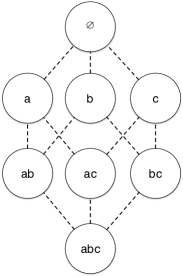
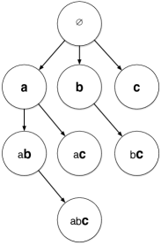
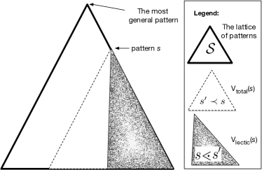
Figure 5: Search space as a lattice (left), DFS of the search space (middle), and the principles of the normalized exploration rate.

Avoiding duplicates in the tree using permutation unification (PU).

The permutation unification is a solution that enables to keep a unique node for all duplicates of a pattern that can be expanded within several branches of the tree. This is inspired from Permutation AMAF of [29], a method used in traditional MCTS algorithms to update all the nodes that can be concerned by a play-out. A unified node no longer has a single parent but a list of all duplicates’ parent. This list will be used when back-propagating a reward.

This method is detailed in Algorithm 4.2. Consider that the node $s_{exp}$ has been chosen as an expansion of the selected node $s_{sel}$. The tree generated so far is explored for finding $s_{exp}$ elsewhere in the tree: If $s_{exp}$ is not found, we proceed as usual; otherwise $s_{exp}$ becomes a pointer to the duplicate node in the tree. In our MCTS implementation, we will simply use a hash map to store each pattern and the node in which is has been firstly encountered.

Algorithm 4.2.

1:$H\leftarrow$ new Hashmap()

2:function Expand($s_{sel}$)

3:     randomly choose $s_{exp}$ from non expanded children of $s_{sel}$

4:     if $(node\leftarrow H.get(s_{exp}))\not=null$ then

5:         $node.parents.add(s_{sel})$

6:         $s_{exp}\leftarrow node$

7:     else

8:         $s_{exp}.parents\leftarrow$ new List()

9:         $s_{exp}.parents.add(s_{sel})$

10:         $H.put(s_{exp},s_{exp})$ $\triangleright$ A pointer on the unique occurrence of $s_{exp}$

11:end if

12:add new child $s_{exp}$ to $s_{sel}$ in the tree $\triangleright$ Expand $s_{sel}$ with $s_{exp}$

13:return $s_{exp}$

14:end function

The permutation unification principle.

4.3 The RollOut method

From the expanded node $s_{exp}$ a simulation is run (RollOut). With standard MCTS, a simulation is a random sequence of actions that leads to a terminal node: A game state from which a reward can be computed (win/loss). In our settings, it is not only the leaves that can be evaluated, but any pattern $s$ encountered during the simulation. Thus, we propose to define the notion of path (the simulation) and reward computation (which nodes are evaluated and how these different rewards are aggregated) separately.

Definition 14 (Path policy).

Let $s_{1}$ the node from which a simulation has to be run (i.e., $s_{1}=s_{exp}$). Let $n\geq 1\in\mathbb{N}$, we define a path $p(s_{1},s_{n})=\{s_{1},\dots,s_{n}\}$ as a chain in the lattice $(\mathcal{S},\prec)$, i.e., an ordered list of patterns starting from $s_{1}$ and ending with $s_{n}$ such that $\forall i\in\{1,\dots,n-1\},s_{i+1}$ is a (not necessarily direct) refined pattern of $s_{i}$.

• naive-roll-out: a path of direct refinements is randomly created with length $pathLength\in\mathbb{N}^{+}$ a user-defined parameter.

• direct-freq-roll-out: The path is extended with a randomly chosen restriction until it meets an infrequent pattern $s_{n+1}$ using the direct refinement operator. Pattern $s_{n}$ is a leaf of the tree in our settings.

• large-freq-roll-out overrides the direct-freq-roll-out policy by using specializations that are not necessarily direct. Several actions are added instead of one to create a new element of the path. The number of added actions is randomly picked in $(1,...,jumpLength)$ where $jumpLength$ is given by the user ($jumpLength=1$ gives the previous policy). This techniques allows to visit deep parts of the search space with shorter paths.

Definition 15 (Reward aggregation policy).

Let $s_{1}$ be the node from which a simulation has been run and $p(s_{1},s_{n})$ the associated random path. Let $\mathcal{E}\subseteq p(s_{1},s_{n})$ be the subset of nodes to be evaluated. The aggregated reward of the simulation is given by: $\Delta=aggr(\{\varphi(s)\forall s\in\mathcal{E}\})\in[0;1]$ where $aggr$ is an aggregation function. We define several reward aggregation policies:

• terminal-reward: $\mathcal{E}=\{s_{n}\}$ and $aggr$ is the identity function.

• random-reward: $\mathcal{E}=\{s_{i}\}$ with a random $1\leq i\leq n$ and $aggr$ is the identity function.

• max-reward: $\mathcal{E}=p(s_{1},s_{n})$ and $aggr$ is the $max(.)$ function

• mean-reward: $\mathcal{E}=p(s_{1},s_{n})$ and $aggr$ is the $mean(.)$ function.

• top-k-mean-reward: $\mathcal{E}=$ top-k$(p(s_{1},s_{n}))$, $aggr$ is the $mean(.)$ function and top-k(.) returns the $k$ elements with the highest $\varphi$.

A basic MCTS forgets any state encountered during a simulation. This is not optimal for single player games as relate [8]: A pattern with a high $\varphi$ should not be forgotten as we might not expand the tree enough to reach it. We propose to consider several memory strategies.

Definition 16 (Roll-out memory policy).

A roll-out memory policy specifies which of the nodes of the path $p=(s_{1},s_{n})$ shall be kept in an auxiliary data structure $M$.

• no-memory: Any pattern in $\mathcal{E}$ is forgotten.

• all-memory: All evaluated patterns in $\mathcal{E}$ are kept.

• top-k-memory: A list $M$ stores the best $k$ patterns in $\mathcal{E}$ w.r.t. $\varphi(.)$.

This structure $M$ will be used to produce the final pattern set.

4.4 The Update method

The backpropagation method updates the tree according to a simulation. Let $s_{sel}$ be the selected node and $s_{exp}$ its expansion from which the simulation is run: This step aims at updating the estimation $Q(.)$ and the number of visits $N(.)$ of each parent of $s_{exp}$ recursively. Note that $s_{exp}$ may have several parents when we enable permutation unification (PU). The number of visits is always incremented by one. We consider three ways of updating $Q(.)$:

• mean-update: $Q(.)$ is the average of the rewards $\Delta$ back-propagated through the node so far (basic MCTS).

• max-update: $Q(.)$ is the maximum reward $\Delta$ back-propagated through the node so far. This strategy enables to identify a local optimum within a part of the search space that contains mostly of uninteresting patterns. Thus, it gives more chance for this area to be exploited in the next iterations.

• top-k-mean-update: $Q(.)$ average of the $k$ best rewards $\Delta$ back-propagated through the node so far. It gives a stronger impact for the parts of the search space containing several local optima.

mean-update is a standard in MCTS techniques. We introduce the max-update and top-k-mean-update policies as it may often happen that high-quality patterns are rare and scattered in the search space. The mean value of rewards from simulations would converge towards 0 (there are too many low quality subgroups), whereas the maximum value (and top-k average) of rewards enables to identify the promising parts of the search space.

4.5 Search end and result output

There are two ways a MCTS ends: Either the computational budget is reached (number of iterations) or the tree is fully expanded (an exhaustive search has been possible, basically when the size of the search space is smaller than the number of iterations). Indeed, the number of tree nodes equals the number of iterations that have been performed. It remains now to explore this tree and the data structure $M$ built by the memory policy to output the list of diverse and non-redundant patterns.

Let $\mathcal{P}=T\cup M$ be a pool of patterns, where $T$ is the set of patterns stored in the nodes of the tree. The set $\mathcal{P}$ is totally sorted w.r.t. $\varphi$ in a list $\Lambda$. Thus, we have to pick the $k$-best diverse and non-redundant subgroups within this large pool of nodes $\Lambda$ to return the result set of subgroups $\mathcal{R}\subseteq\mathcal{P}$. For that, we choose to implement $filter(.)$ in a greedy manner as done by[53, 10]. $\mathcal{R}=filter(\mathcal{P})$ as follows: A post-processing that filters out redundant subgroups from the diverse pool of patterns $\Lambda$ based on the similarity measure $sim$ and the maximum similarity threshold $\Theta$. Recursively, we poll (and remove) the best subgroup $s^{*}$ from $\Lambda$, and we add $s^{*}$ to $\mathcal{R}$ if it is not redundant with any subgroup in $\mathcal{R}$. It can be shown easily that $redundancy(\mathcal{R})=0$.

Applying $filter(.)$ at the end of the search requires however that the pool of patterns $\mathcal{P}$ has a reasonable cardinality which may be problematic with MCTS in term of memory. The allowed budget always enables such post-processing in our experiments (up to one million iterations).

5 Related work

SD aims at extracting subgroups of individuals for which the distribution on the target variable is statistically different from the whole (or the rest of the) population [[34, 55]]. Two similar notions have been formalized independently and then unified by [45]: Contrast set mining and emerging patterns. Close to SD, redescription mining aims to discover redescriptions of the same group of objects in different views [51]. Exceptional model mining (EMM) was first introduced by [38] (see a comprehensive survey by [17]). EMM generalizes SD dealing with more complex target concepts: There are not necessarily one but several target variables to discriminate. EMM seeks to elicit patterns whose extents induce a model that substantially deviates from the one induced by the whole dataset.

First exploration methods that have been proposed for SD/EMM are exhaustive search ensuring that the best subgroups are found, e.g. [34, 55, 31, 3]. Several pruning strategies have been used to avoid the exploration of uninteresting parts of the search space. These pruning strategies are usually based on the monotonic (or anti-monotonic) property of the support or upper bounds on the quality measure [[26, 33]]. To the best of our knowledge, the most efficient algorithms are (i) SD-MAP* from [3] which is based on the FP-growth paradigm [[27]] and (ii) an exhaustive exploration with optimistic estimates on different quality measures [[39]]. When an exhaustive search is not possible, heuristic search can be used. The most widely used techniques in SD and EMM are beam search, evolutionary algorithms and sampling methods. Beam search performs a level-wise exploration of the search space: A beam of a given size (or dynamic size for recent work) is built from the root of the search space. This beam only keeps the most promising subgroups to extend at each level [[36, 44, 53]]. The redundancy issue due to the beam search is tackled with the pattern skyline paradigm by [54], and with a ROC-based beam search variant for SD by [42]. Another family of SD algorithms relies on evolutionary approaches. They use a fitness function to select which individuals to keep at the next generated population. SDIGA, from [15], is based on a fuzzy rule induction system where a rule is a pattern in disjunctive normal form (DNF). Other approaches have been then proposed, generally ad-hoc solutions suited for specific pattern languages and selected quality measures [[47, 46, 14]].

Finally, pattern sampling techniques are gaining interest. [43] employ controlled direct pattern sampling (CDPS). It enables to create random patterns with the help of a procedure based on a controlled distribution as did [9]. This idea was extended by [7] for a particular EMM problem to discover exceptional models induced by attributed graphs. Pattern sampling is attractive as it supports direct interactions with the user for using his/her preferences to drive the search. Besides, with sampling methods, a result is available anytime. However, traditional sampling methods used in pattern mining need a given probability distribution over the pattern space: This distribution depends on both the data and the measures [[9, 43]]. Each iteration is independent and consists of drawing a pattern given this probability distribution. Moreover, these probability distributions exhibit the problem of the long tail: There are many more uninteresting patterns than interesting ones. Thus, the probability to draw an uninteresting pattern is still high, and not all local optima may be drawn: There are no guaranties on the diversity of the result set. Recently, the sampling algorithm Misere has been proposed by [24, 20, 21]. Contrary to the sampling method of Moens and Boley, Misere does not require any probability distribution. It is agnostic of the quality measure but it still employs a discretization of numerical attribute in a pre-processing task. To draw a pattern, Misere randomly picks an object in the data, and thus it randomly generalizes it into a pattern that is evaluated with the quality measure. Each draw is independent and thus the same pattern can be drawn several times. Finally, MCTS samples the search space without any assumption about the data and the measure. Contrary to sampling methods, it stores the result of the simulations of the previous iterations and it uses this knowledge for the next iterations: The probability distribution is learned incrementally. If given enough computation budget, the exploration/exploitation trade-off guides the exploration to all local optima (an exhaustive search). To the best of our knowledge, MCTS has never been used in pattern mining, however, [23] designed the algorithm FUSE (Feature UCT Selection) which extends MCTS to a feature selection problem. This work aims at selecting the features from a feature space that are the more relevant w.r.t. the classification problem. For that, Gaudel and Sebag explore the powerset of the features (i.e., itemsets where the items are the features) with a MCTS method to find the sets of features that minimize the generalization error. Each node of the tree is a subset of feature, and each action consists of adding a new feature in the subset of features. The authors focus on reducing the high branching factor by using UCB1-Tuned and RAVE introduced by [25]. The latter enables to select a node even if it remains children to expand. The aim of FUSE is thus to return the best subset of features (the most visited path of the tree), or to rank the features with the RAVE score.

6 Empirical evaluation on how to parameterize mcts4dm

Our MCTS implementation for pattern mining, called mcts4dm is publicly available. As there are many ways to configure mcts4dm, we propose first to study the influence of the parameters on runtime, pattern quality and diversity. We both consider benchmark and artificial data. The experiments were carried out on an Intel Core i7 CPU 4 Ghz machine with 16 GB RAM running under Windows 10.

6.1 Data

Firstly, we gathered benchmark datasets used in the recent literature of SD and EMM, that is, from [53, 16, 51, 52, 18]. Table 3 lists them, mainly taken from the UCI repository, and we provide some of their properties.

Secondly, we used a real world dataset from neuroscience. It concerns olfaction (see Table 3).This data provides a very large search space of numerical attributes (more details on the application are presented by [10]).

Finally, to be able to specifically evaluate diversity, a ground-truth is required. Therefore, we create an artificial data generator to produce datasets where patterns with a controlled WRAcc are hidden. The generator takes the parameters given in Table 4 and it works as follow. A data table with nominal attributes is generated with a binary target. The number of objects, attributes and attributes values are controlled with the parameters $nb\_obj$, $nb\_attr$ and $domain\_size$. Our goal is to hide $nb\_patterns$ patterns in noise: We generate random descriptions of random lengths $Ground=\{d_{i}~{}|~{}i\in[1,nb\_patterns]\}$. For each pattern, we generate $pattern\_sup$ objects positively labeled with a probability of $1-noise\_rate$ to be covered by the description $d_{i}$, and $noise\_rate$ for not being covered. We also add $pattern\_sup\times out\_factor$ negative examples for the pattern $d_{i}$: It will allow patterns with different WRAcc. Finally, we add random objects until we reach a maximum number of transactions $nb\_obj$.

Table 3: Benchmark datasets experimented on in the SD and EMM literature.

Name	# Objects	# Attributes	Type of attributes	Target attribute
Bibtex	7,395	1,836	Binary	TAG_statphys23
BreastCancer	699	9	Numeric	Benign
Cal500	502	68	Numeric	Angry-Agressive
Emotions	594	72	Numeric	Amazed-suprised
Ionosphere	352	35	Numeric	Good
Iris	150	4	Numeric	Iris-setosa
Mushroom	8,124	22	Nominal	Poisonous
Nursery	12,961	8	Nominal	class=priority
Olfaction	1,689	82	Numeric	Musk
TicTacToe	958	9	Nominal	Positive
Yeast	2,417	103	Numeric	Class1

Table 4: Parameters of the artificial data generator.

Name	Description	$\mathcal{P}_{small}$	$\mathcal{P}_{medium}$	$\mathcal{P}_{large}$
$nb\_obj$	Number of objects	2,000	20,000	50,000
$nb\_attr$	Number of attributes	5	5	25
$domain\_size$	Domain size per attribute	10	20	50
$nb\_patterns$	Number of hidden patterns	3	5	25
$pattern\_sup$	Support of each hidden pattern	100	100	100
$out\_factor$	Proba. of a pattern labeled $-$	0.1	0.1	0.1
$noise\_rate$	Proba. of a object to be noisy	0.1	0.1	0.1

6.2 Experimental framework

We perform a large pool of experiments to assess this new exploration method for pattern mining. For that, we have designed an experimental framework that enables to test the different combinations of factors for all the strategies we introduced in previous sections. Each experiment are run on the benchmark datasets. An experiment consists in varying a unique strategy parameter while the others are fixed. Since mcts4dm uses random choices, each experiment is run five times and only the mean of the results is discussed.

Default parameters.

For each benchmark dataset, we provide a set of default parameters (Table 5). Indeed, due to the specific characteristics of each dataset, a common set of default parameters is unsuitable. Nevertheless, all datasets share a subset of common parameters:

• The maximum size of the result set is set to $maxOutput=50$.

• The maximum redundancy threshold is set to $\Theta=0.5$.

• The maximum description length is set to $maxLength=5$. This is a widely used constraint in SD that enables to restrict the length of the description, i.e., it limits the number of effective restrictions in the description.

• The quality measure used is $\varphi=WRAcc$ for the first label only.

• The SP-MCTS is used as the default UCB.

• The permutation unification (PU) strategy is used by default.

• The refinement operator for Expand is set to tuned-min-gen-expand.

• The direct-freq-roll-out strategy is used for the Roll-Out

• The reward aggregation policy is set to max-reward.

• The memory policy is set to top-1-memory.

• The update policy is set to max-udpate.

Table 5: The default parameters for each dataset.

Dataset	minSupp	# iterations	Path Policy
Bibtex	50	50k	direct-freq-roll-out
BreastCancer	10	50k	large-freq-roll-out ($jumpLength=30$)
Cal500	10	100k	large-freq-roll-out ($jumpLength=30$)
Emotions	10	100k	large-freq-roll-out ($jumpLength=30$)
Ionosphere	10	50k	large-freq-roll-out ($jumpLength=30$)
Iris	10	50k	large-freq-roll-out ($jumpLength=30$)
Mushroom	30	50k	direct-freq-roll-out
Nursery	50	100k	direct-freq-roll-out
Olfaction	10	100k	large-freq-roll-out ($jumpLength=30$)
TicTacToe	10	100k	direct-freq-roll-out
Yeast	20	100k	large-freq-roll-out ($jumpLength=30$)

List of experiments.

Evaluating mcts4dm is performed with six different batches of experiments:

• Section 6.3 is about the choice of the UCB.

• Section 6.4 deals with the several strategies for the Expand method.

• Section 6.5 presents the leverage of all the possibilities for the RollOut.

• Section 6.6 shows out the impact of the Memory strategy.

• Section 6.7 compares the behaviors of all the strategies for the Update.

• Section 6.8 performs the experiments by varying the computational budget.

• Section 6.9 studies if mcts4dm is able to retrieved a diverse pattern set.

For simplicity and convenience, for each experiment we display the same batch of figures. For each dataset we show (i) the boxplots of the quality measure $\varphi$ of the subgroups in the result set, (ii) the histograms of the runtime and (iii) the boxplots of the description length of the subgroups in the result set depending on the strategies that are used. In this way, the impacts of the strategies are easy to understand.

We do not evaluate memory consumption in this section, as it increases linearly with the number of iterations (to which should be added the number of patterns kept by the memory policy).

6.3 The Select method

The choice of the UCB is decisive, because it is the base of the exploration / exploitation trade off. Indeed, the UCB chooses which part of the search tree will be expanded and explored. We presented four existing UCBs and an adaptation with a normalized exploration rate to take into account an enumeration based on a lectic order (LO). As such, we need to consider also the expand methods (standard, lectic order LO and permutation unification PU) at the same time.

Figure 6 presents the results. Comparing the runtime for all the strategies leads to conclude that there is no difference in the computation of the several UCBs (see Figure 6(a)). Indeed, the impact of the UCBs lies in its computation, and there is no UCB that is more time-consuming than others. The difference we can notice, is that when LO is used, the runtime is lower. This result is expected because with LO, the search space is less large since each subgroup is unique in the search space (this is not due to the chosen UCB). PU has also a smaller search space, but it requires call to updates pointers towards subgroups with the same extent, and requires thus more time.

Figure 6(b) depicts the boxplots of the quality measure of the result set when varying the UCB. The results suggest that the UCB1-Tuned and DFS-UCT lead to weaker quality result for several datasets: On the Cal550, Emotions and Yeast datasets, the quality measures of the result set are worse than the results of other UCBs (see, e.g., Figure 6(b)). This is due to the fact that the search space of these datasets is larger than the other with many local optima, and the UCB1-Tuned is designed to explore less, thus less local optima are found. Besides, the SP-MCTS seems to be more suitable for SD problems: The quality is slightly better than other UCBs for the BreastCancer and Emotions datasets. LO leads to a worse quality in the result set, whereas PU seems to be more efficient.

The use of these different UCBs also do not impact the description length of the subgroups within the result set. For some datasets, the permutation unification leads to longer descriptions (see for instance Figure 6(c)).

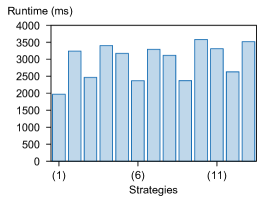
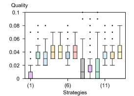
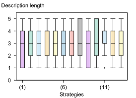
(a) Runtime: BreastCancer	(b) Avg. quality: Emotions	(c) Descr length: Mushroom
Select Policies: (1) DFS-UCT with LO
(2) UCB1 (3) UCB1 with LO (4) UCB1 with PU
(5) SP-MCTS (6) SP-MCTS with LO (7) SP-MCTS with PU
(8) UCB1-Tuned (9) UCB1-Tuned with LO (10) UCB1-Tuned with PU
(11) UCT (12) UCT with LO (13) UCT with PU

Figure 6: Impact of the Select strategy.

6.4 The Expand method

Considering the Expand policy, we introduced three different refinement operators, namely direct-expand, gen-expand and label-expand, and we presented two methods, namely LO and PU, to take into account that several nodes in the search tree are exactly the same. The several strategies we experiment with are given in Figure 7(bottom). Let us consider the leverage on the runtime of these strategies in Figure 7(a). Once again, using LO implies a decrease of the runtime. Conversely, PU requires more time to run. There is very little difference in the runtime when varing the refinement operator: direct-expand is the faster one, and label-expand is more time consuming.

Considering the quality of the result set varying the expand strategies, we can assume that the impact differs w.r.t. the dataset (see Figure 7(b)). Surprisingly, LO improves the quality of the result set for some datasets (e.g. the Iris dataset in Figure 7(b)). This contradicts what we observe in the Emotions dataset of the previous experiment in Section 6.3. Most importantly, the results using label-expand are better than other ones in most of the datasets. Actually, this is due that this expand favors pattern with a better accuracy which is part of the WRAcc.

The description length of the extracted subgroups are quite constant when varying the expand strategies (see Figure 7(c)). With LO, the description lengths are slightly smaller than with other strategies.

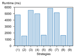
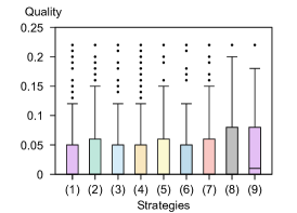
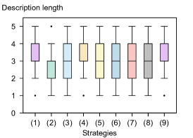
(a) Runtime: Nursery
	(b) Avg. quality: Iris	(c) Descr length: Mushroom
(1) direct-expand (2) direct-expand with LO (3) direct-expand with PU
(4) gen-expand (5) gen-expand with LO (6) gen-expand with PU
(7) label-expand (8) label-expand with LO (9) label-expand with PU

Figure 7: Impact of the Expand strategy.

6.5 The RollOut method

For the RollOut step we derived several strategies that combine both the path policy and the reward aggregation policy in Table 6. Clearly, the experiments show that the runs using the direct refinement operator (naive-roll-out and direct-freq-roll-out) are time consuming (see Figure 8(a)). In the BreastCancer data, the runtime are twice longer with the direct refinement operator than with the large-freq-roll-out path policy. In other datasets (e.g., Ionosphere or Yeast), the runtime is even more than 3 minutes (if the run lasts more than 3 minutes to perform the number of iterations, the run is ignored). Besides, it is clear that the random-reward aggregation policy is less time consuming than other strategies. Indeed, with random-reward, the measure of only one subgroup within the path is computed, thus it is faster.

Figure 8(b) is about the quality of the result set. The naive-roll-out and direct-freq-roll-out path policies lead to the worst results. Besides, the quality of the result set decreases with the random-reward reward aggregation policy in other datasets (e.g., Emotions). Basically, these strategies evaluate only random nodes and thus they are not able to identify the promising parts of the search space. Finally, there are not large differences between other strategies.

As can be seen in Figure 8(c), the description length of the subgroups is not very impacted by the strategies of the Roll-Out step. The results of the random-reward reward aggregation policy are still different from other strategies: The description length is smaller for the Mushroom dataset. Using large-freq-roll-out with $jumpLength=100$ leads to smaller descriptions for the Mushroom dataset. Finally, the description length is not or almost not influenced by the Roll-Out strategies.

Table 6: The list of strategies used to experiment with the RollOut method.

Strategy	Path Policy	Reward Aggregation Policy
(1)	naive-roll-out ($pathLength=20$)	terminal-reward
(2)	direct-freq-roll-out	max-reward
(3)	direct-freq-roll-out	mean-reward
(4)	direct-freq-roll-out	top-2-mean-reward
(5)	direct-freq-roll-out	top-5-mean-reward
(6)	direct-freq-roll-out	top-10-mean-reward
(7)	direct-freq-roll-out	random-reward
(8)	large-freq-roll-out ($jumpLength=10)$	max-reward
(9)	large-freq-roll-out ($jumpLength=10)$	mean-reward
(10)	large-freq-roll-out ($jumpLength=10)$	top-2-mean-reward
(11)	large-freq-roll-out ($jumpLength=10)$	top-5-mean-reward
(12)	large-freq-roll-out ($jumpLength=10)$	top-10-mean-reward
(13)	large-freq-roll-out ($jumpLength=10)$	random-reward
(14)	large-freq-roll-out ($jumpLength=20)$	max-reward
(15)	large-freq-roll-out ($jumpLength=20)$	mean-reward
(16)	large-freq-roll-out ($jumpLength=20)$	top-2-mean-reward
(17)	large-freq-roll-out ($jumpLength=20)$	top-5-mean-reward
(18)	large-freq-roll-out ($jumpLength=20)$	top-10-mean-reward
(19)	large-freq-roll-out ($jumpLength=20)$	random-reward
(20)	large-freq-roll-out ($jumpLength=50)$	max-reward
(21)	large-freq-roll-out ($jumpLength=50)$	mean-reward
(22)	large-freq-roll-out ($jumpLength=50)$	top-2-mean-reward
(23)	large-freq-roll-out ($jumpLength=50)$	top-5-mean-reward
(24)	large-freq-roll-out ($jumpLength=50)$	top-10-mean-reward
(25)	large-freq-roll-out ($jumpLength=50)$	random-reward
(26)	large-freq-roll-out ($jumpLength=100)$	max-reward
(27)	large-freq-roll-out ($jumpLength=100)$	mean-reward
(28)	large-freq-roll-out ($jumpLength=100)$	top-2-mean-reward
(29)	large-freq-roll-out ($jumpLength=100)$	top-5-mean-reward
(30)	large-freq-roll-out ($jumpLength=100)$	top-10-mean-reward
(31)	large-freq-roll-out ($jumpLength=100)$	random-reward

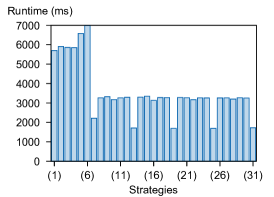
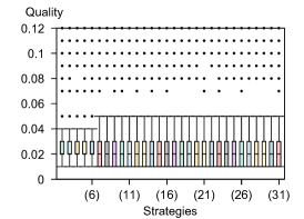
(a) Runtime: BreastCancer	(b) Avg. quality: Mushroom	(c) Descr length: Mushroom

Figure 8: Impact of the Roll-Out strategy.

6.6 The Memory method

We derived six strategies for the Memory step given in Figure 9(bottom). Obviously, the all-memory policy is slower than other strategies because all the nodes within the path of the simulation have to be stored (see Figure 9(a)). Conversely, the no-memory policy is the fastest strategy. The runtimes of the top-k-memory policies is comparable.

Figure 9(b) shows that the quality of the result set is impacted by the choice of the memory policies. We can observe that the no-memory is clearly worse than other strategies. Indeed, in the Emotion dataset, the best subgroups are located more deeper in the search space, thus, if the solutions encountered during the simulation are not stored it would be difficult to find them just be considering the subgroups that are expanded in the search tree. Surprisingly, the all-memory policy does not lead to better result. In fact the path generated during a simulation contains a lot of redundant subgroups: Storing all these nodes is not required to improve the quality of the result set. Only few subgroups within the path are related to different local optima.

As expected in Figure 9(c), the descriptions of the subgroups obtained with the no-memory policy are smaller than those of other strategies. Indeed, with the no-memory policy, the result sets contains only subgroups that are expanded in the search tree, in other words, the subgroups obtained with the Expand step.

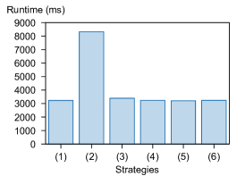
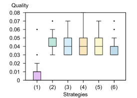
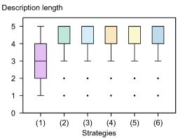
(a) Runtime: Ionosphere	(b) Avg. quality: Emotions	(c) Descr. length: BreastCancer
(1) no-memory (2) all-memory (3) top-1-memory
(4) top-2-memory (5) top-5-memory (6) top-10-memory

Figure 9: Impact of the Memory strategy.

6.7 The Update method

Figure 10(bottom) presents the different strategies we use to implement the Update step. The goal of this step is to back-propagate the reward obtained by the simulation to the parent nodes. The runtime of these strategies are comparable (see Figure 10(a)). However, we notice that the top-k-mean-update policy is a little more time consuming. Indeed, we have to maintain a list for each node within the built tree that stores the top-k best rewards obtained so far.

Figure 10(b) shows the quality of the result set when varying the Update policies. For most of the datasets, since the proportion of local optima is very low within the search space, the max-update is more efficient than the mean-update. Indeed, using the max-update enables to keep in mind that there is an interesting pattern that is reachable from a node. However, Figure 10(b) presents the opposite phenomena: The mean-update policy leads to a better result. In fact, since there are a lot of local optima in the Ionosphere dataset, the mean-update can find the areas with lots of interesting solutions. Moreover, using the top-k-mean-update leads to the mean-update when $k$ increases.

The description of the subgroups in the result set is comparable when varying the policies of the Update method (see Figure 10(c)). Indeed, the aim of the Update step is just to back-propagate the reward obtained during the simulation to the nodes of the built tree to guide the exploration for the following iterations. This step does not have a large influence on the length of the description of the subgroups.

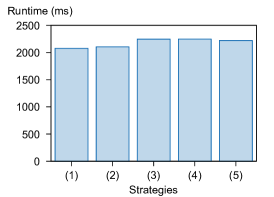
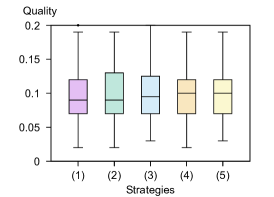
(a) Runtime: TicTacToe	(b) Avg. quality: Ionosphere	(c) Descr length: Iris
(1) max-update (2) mean-update (3) top-2-mean-update
(4) top-5-mean-update (5) top-10-mean-update

Figure 10: Impact of the Update strategy.

6.8 The number of iterations

We study the impact of different computational budgets allocated to mcts4dm, that is, the maximum number of iterations the algorithm can perform. As depicted in Figure 11(a), the runtime is linear with the number of iterations. The x-axis is not linear w.r.t. the number of iterations, please refer to the bottom of Figure 11 to know the different values of the number of iterations.

Moreover, as expected, the more iterations, the better the quality of the result set. Figure 11(b) shows that a larger computational budget leads to a better quality of the result set, but, obviously, it requires more time. Thus, with this exploration method, the user can have some results anytime. For the BreastCancer dataset, the quality decreases from 10 to 100 iterations: This is due to the fact that with 10 iterations there are less subgroups extracted (12 subgroups) than with 100 iterations (40 subgroups), and the mean quality of the result set with 100 iterations contains also subgroups with lower quality measures.

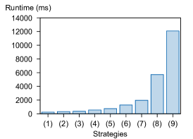
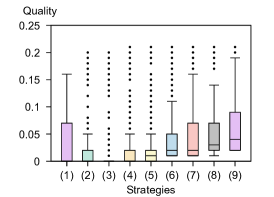
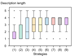
(a) Runtime: Cal500	(b) Avg. quality: BreastCancer	(c) Descr length: Nursery
(strategy)#iterations: (1)10 (2)50 (3)100 (4)500 (5)1K (6)5K (7)10K (8)50K (9)100K

Figure 11: Impact of the maximal budget (number of iterations).

6.9 Evaluating pattern set diversity when a ground truth is known

Artificial datasets are generated according to default parameters given in Table 4. Then, we study separately the impact of each parameter on the ability to retrieve the hidden patterns with our MCTS algorithm. After a few trials, we use the following default MCTS parameters: The single player UCB (SP-MCTS) for the select policy; the label-expand policy with PU activated; the direct-freq-roll-out policy for the simulations, the max-update policy as aggregation function of the rewards of a simulation, the top-10-memory policy and finally the max-update policy for the back-propagation.

The ability to retrieve hidden patterns is measured with a Jaccard coefficient between the support of the hidden patterns and the one discovered by the algorithm:

Definition 17 (Evaluation measure).

Let $\mathcal{H}$ be the set of hidden patterns, and $\mathcal{F}$ the set of patterns found by an MCTS mining algorithm, the quality, of the found collection is given by:

$$qual(\mathcal{H},\mathcal{F})=avg_{\forall h\in\mathcal{H}}(max_{\forall f\in\mathcal{F}}(Jaccard(ext(h),ext(f))))$$

that is, the average of the quality of each hidden pattern, which is the best Jaccard coefficient with a found pattern. We thus measure here the diversity. It is a pessimistic measure in the sense that it takes its maximum value $1$ iff all patterns have been completely retrieved.

It can be noticed that we do not use the Definition 6 for diversity: As a ground truth is available, we opt for a measure that quantifies its recovering.

Varying the noise parameter. We start with the set of parameters $\mathcal{P}_{small}$. The results are given in Figure 12 with different minimal support values (used during the expand step and the simulations). Recall that a hidden pattern is random set of symbols $attribute=value$ when dealing with nominal attributes, repeated in $pattern\_sup$ object descriptions: The noise makes that each generated object description may not support the pattern. Thus, the noise directly reduces the support of a hidden pattern: increasing the noise requires to decrease the minimal support of the algorithm. This is clearly observable on the different figures. When the minimum support is set to the same value as the support of the hidden patterns ($minSupp=100$), the noise has a strong impact and it is difficult to retrieve the hidden patterns, even when the whole tree (of frequent patterns) has been expanded. Reducing the minimal support to $1$ makes the search very resistant to noise. Note that when two lines exactly overlaps, it means that the search space of frequent patterns was fully explored: MCTS performed an exhaustive search.

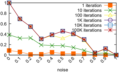
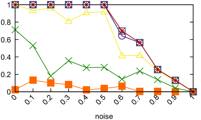
(i) $minSup=100$	(ii) $minSupp=50$
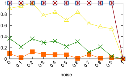
(iii) $minSup=10$

Figure 12: Ability to retrieve hidden patterns ($qual(\mathcal{H},\mathcal{F})$ in Y-axis) when introducing noise and mining with different minimum supports $minSup$.

Varying the out factor parameter. Each pattern is inserted in $pattern\_sup$ transactions (or less when there is noise) as positive examples (class label $+$). We also add $pattern\_sup\times out\_factor$ negative examples (class label $-$). When $out\_factor=1$, each pattern appears as much in positive and negative examples. This allows to hide patterns with different quality measure, and especially different $WRAcc$ measures. The Table LABEL:fig:artificial2 (row (1)) shows that this parameter has no impact: patterns of small quality are retrieved easily in a small number of iterations. The UCB hence drives the search towards promising parts that have the best rewards.

Varying the number of hidden patterns. We claim that the UCB will guide the search towards interesting parts (exploitation) but also unvisited parts (exploration) of the search space. It follows that all hidden patterns should be retrieved and well retrieved. We thus vary the number of random patterns between $1$ and $20$ and observe that they are all retrieved (Table LABEL:fig:artificial2 (row (2))). When increasing the number of hidden more patterns, retrieving all of them requires more iterations in the general case.

Varying the support size of the hidden patterns. Patterns with a high support (relative to the total number of objects) should be easier to be retrieved as a simulation has more chance to discover them, even partially. We observe that patterns with small support can still be retrieved but it requires more iterations to retrieve them in larger datasets (Table LABEL:fig:artificial2 (row (3))).

Varying the number of objects. The number of objects directly influences the computation of the support of each node: Each node stores a projected database that lists which objects belong to the current pattern. The memory required for our MCTS implementation follows a linear complexity w.r.t. the number of iterations. This complexity can be higher depending on the chosen memory policy (e.g. in these experiments, the top-10 memory policy was chosen). The time needed to compute the support of a pattern is higher for larger dataset, but it does not change the number of iterations required to find a good result. This is reported in (Table LABEL:fig:artificial2 (row (4))). Run times will be discussed later.

Varying the number of attributes and the size of attributes domains. These two parameters directly determine the branching factor of the exploration tree. It takes thus more iterations to fully expand a node and to discover all local optima. Here again, all patterns are well discovered but larger datasets require more iterations (Table LABEL:fig:artificial2 (row (5) and (6))).

Table 7: Evaluation of the ability to retrieve hidden patterns in artificial data generated according to different parameters (average of 5 runs for each point). $qual(\mathcal{H},\mathcal{F})$ in Y-axis, parameters given in the first columns as X-axis.

	$\mathcal{P}_{medium}$	$\mathcal{P}_{large}$
(1) $out\_factor$
(2) $nb\_patterns$
(3) $pattern\_sup$
(4) $nb\_obj$
(5) $nb\_attr$
(6) $domain\_size$
	$\mathcal{P}_{medium}$	$\mathcal{P}_{large}$
Legend:

7 Comparisons with existing algorithms

We compare mcts4dm to other SD approaches (exhaustive search, beam search, genetic algorithms and sampling) in terms of computational time, diversity and redundancy of the pattern set, and memory usage. In addition to the benchmark data we used in the previous section, we generate 5 new artificial datasets for which parameters are given in Table 8. In this empirical study, we consider a timeout of 5 minutes that is enough to capture the behavior of the algorithms that are not based on a computational budget, such as SD-Map or beam search approaches. Indeed, mcts4dm and sampling methods use a computational budget.

Table 8: Parameters of the artificial data generator. The format of name of the data is given by their parameters by $[nb\_obj]$_$[nb\_attr]$_$[domain\_size]$.

Name	5000_10_200	5000_50_50	5000_50_200	20000_10_200	20000_50_200
$nb\_obj$	5,000	5,000	5,000	20,000	20,000
$nb\_attr$	10	50	50	10	50
$domain\_size$	200	50	200	200	200
$nb\_patterns$	5	5	5	5	5
$pattern\_sup$	200	200	200	200	200
$out\_factor$	0.05	0.05	0.05	0.05	0.05
$noise\_rate$	0.05	0.05	0.05	0.05	0.05

Table 9: Diversity in the result set for artificial data. The value is the $qual(\mathcal{H},\mathcal{F})$ where $\mathcal{H}$ is the set of hidden patterns in the artificial data and $\mathcal{F}$ is the set of found patterns by the algorithm The character ’-’ means that the algorithm exceeds the time limit of 5 minutes.

Data	$minSupp$	SD-Map	mcts4dm							BeamSearch			Misere							SSDP
			1K	5K	10K	50K	100K	500K	1,000K	10	100	500	1K	5K	10K	50K	100K	500K	1,000K	100	500	1K	5K	10k
5000_10_200	50	1	1	1	1	1	1	1	1	1	0.38	1	1	1	1	1	1	1	1	0.72	0.72	0.72	0.72	0.72
5000_50_50	50	-	0.82	1	1	1	1	-	-	0.99	1	-	0.73	0.94	0.93	0.99	0.99	0.99	1	0.48	0.72	0.72	0.72	0.72
5000_50_200	50	-	1	1	1	1	1	1	1	1	1	-	0.7	0.89	0.97	0.98	0.98	0.99	1	0.68	0.72	0.72	0.72	0.72
20000_10_200	100	1	1	1	1	1	1	1	1	1	1	-	0.77	0.89	0.96	0.97	1	1	-	0.73	0.73	0.73	0.72	-
20000_50_200	100	-	0.69	1	1	1	-	-	-	-	-	-	0.6	0.86	0.87	0.95	0.98	-	-	0.61	0.72	0.72	0.72	-

7.1 SD-Map

SD-Map*, an improvement of SD-Map, is considered as the most efficient exhaustive method for subgroup discovery [[4, 3]]. It employs the FP-Growth principle to enumerate the search space [[28]]. It operates a greedy discretization as a pre-processing step to handle numerical data. It can consider several quality measures to evaluate the interestingness of a subgroup ($WRAcc$, $F1$ score, etc.). The source code is available at http://www.vikamine.org.

Runtime. SD-Map* is very efficient when dealing with dataset of reasonable search space size. We empirically study the scalability of this algorithm compared to those of mcts4dm for several numbers of iterations. Figure 13 (a) displays the runtime of SD-Map* on the Mushroom dataset when varying the minimum support threshold. Clearly, for high minimum support thresholds, SD-Map* is able to provide the results quickly. However, the runtime is exponential w.r.t. this threshold, and thus this algorithm cannot be applied to extract small subgroups. Conversely, mcts4dm is tractable for very low minimum support thresholds: Many iterations can be performed. Figure 13 (b) displays the runtimes for the Ionosphere data and once again mcts4dm is able to perform lots of iteration in a linear time w.r.t. the minimum support threshold whereas SD-Map* fails.

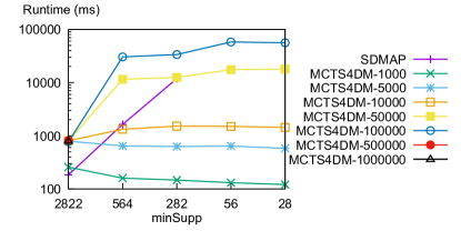
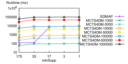
(a) Mushroom	(b) Ionosphere

Figure 13: Runtime of SD-Map and mcts4dm when varying minSupp.

Redundancy and diversity in the result set. SD-Map* is an exhaustive search, thus the diversity of the result set is either perfect if the run can finish or null: Table 9 gives the diversity using the formula of Definition 17 on artificial data since the ground truth is known. However when dealing with numerical attributes, SD-Map* does not ensure a perfect diversity anymore. Indeed, since it handles numerical attributes by performing a discretization in a pre-processing step, there is no guarantee to extract the best patterns. For example, in the BreastCancer dataset, the quality measure of the best subgroup extracted by SD-Map* is 0.18 whereas mcts4dm has found a subgroup whose quality measure is 0.21 with $50,000$ iterations in only $0.213$ms. Figure 14 (a) and Figure 14 (b) show the redundancy of the result set (computed with the formula in Definiton 5) extracted on the Mushroom dataset respectively with $minSupp=264$ and $minSupp=282$. Obviously, the lower the maximum similarity threshold $\Theta$, the more redundant the result set. Compared to SD-Map*, mcts4dm produces few redundancy when performing few iterations, but few iterations are not enough to provide good results: The more iterations, the more redundancy. Surprisingly, the result set of mcts4dm can be more redundant than those of SD-Map* that represents our baseline. Indeed, the set of redundant patterns for the main local optima is larger than for other small local optima, i.e., there are many more patterns that are similar with the main local optima than with small local optima. Since mcts4dm generally finds at first the main local optima, the redundancy measure is higher than those of SD-Map* because there are, in proportion, more redundant subgroups in the result set than local optima. When $minSupp$ decreases, SD-Map* becomes more redundant compared to some mcts4dm runs.

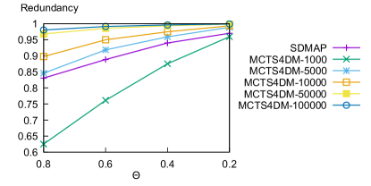
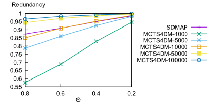
(a) minSupp = 564	(b) minSupp=282

Figure 14: The redundancy in the result set for the Mushroom data varying $\Theta$.

Memory usage. Figure 15 (a) displays the memory usage of our algorithm mcts4dm on the Mushroom data with different numbers of iterations. As expected, the more iterations, the higher the memory usage. It grows linearly with the number of iterations (the creation of the storage structures avoids to see the linear growth of the memory during the first iterations). Figure 15 (b) displays the memory usage when varying the minimum support threshold in the Mushroom dataset for all the considered algorithms. Here, we only discuss the case of SD-Map* compared to mcts4dm. Although SD-Map* is an exhaustive search, its memory usage is similar to (but slightly lower than) those of mcts4dm with $100k$ iterations. It confirms that the implementation of SD-Map* is efficient.

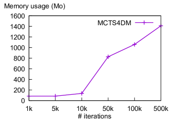
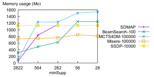
(a) mcts4dm	(b) All algorithms

Figure 15: The memory usage in the Mushroom dataset.

7.2 Beam search

The beam search strategy is the most popular heuristic method in subgroup discovery. Cortana is a tool that enables to run SD tasks with beam search approaches and its source code is available at http://datamining.liacs.nl/cortana.html. Beam search, originally introduced in [40], is a greedy method that partially explores the search space with several hill climbings run in parallel. It proceeds in a level-wise approach considering at each level the best subgroups to extend at the next level. The number of subgroups that are kept to be extended at the next level is called the beam width.

Runtime. By definition, beam search can only find, yet very quickly, local optima reachable from the most general pattern with a hill climbing. Figure 16 shows the runtimes with different beam widths. Obviously, the larger the beam width, the longer the runtimes. However, even with a beam width of 500, the runtime is lower than those of mcts4dm with $100k$ iterations. This is due to the greedy nature of beam search that expands subgroups only if the quality measure increases. However, the local optima that are located deeper in the search space are often missed since the quality measure is not monotone. For large data, such as Bibtex, the beam search is not tractable since it is required to expand all the first level of the search tree to build up the beam. Thus, in our settings, the timeout of 5 minutes is reached with beam search whereas mcts4dm can proceed to $100k$ iterations in 4 minutes.

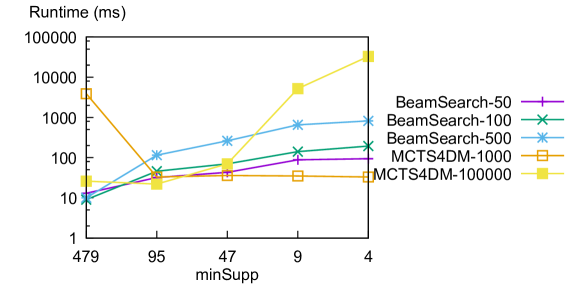
Figure 16: Runtime of the beam search exploration and mcts4dm when varying minSupp in the tictactoe dataset.

Redundancy and diversity in the result set. Due to the greedy approach of the beam search, the redundancy in the result set is the main problem. Figure 17 (a) compares the redundancy in the TicTacToe data obtained with several beam searches and with mcts4dm. Clearly, the beam search leads to a more redundant result set than mcts4dm. This remark holds for all data we experimented with. For example, in the Olfaction dataset, there is a high difference in the redundancy in the result set obtained with a beam search as well (Figure 17 (b)). Besides this high redundancy in the result set with a beam search, the diversity is not as good as with mcts4dm. Even if in Table 9, the beam search extracts the local optima for some datasets, it may require large beam widths that are time consuming. Figure 18 illustrates the diversity for the BreastCancer data with $\Theta=0.2$. With $100k$ iterations, mcts4dm leads to a much more diverse result set than a beam search.

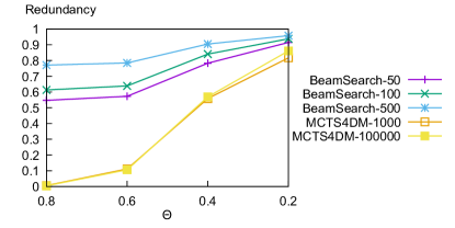
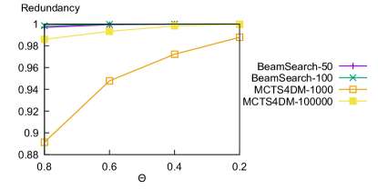
(a) TicTacToe ($minSupp=47$)	(b) Olfaction ($minSupp=84$)

Figure 17: The redundancy in the result set for the TicTacToe and Olfaction data for the beam search strategy.

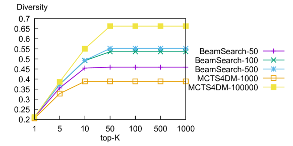
Figure 18: The diversity of the result set in BreastCancer data when $\Theta=0.2$.

Memory consumption. The size of the set of patterns extracted with a beam search is generally lower than the size of the set of patterns obtained with tens of thousands iterations with mcts4dm. Thus, the memory usage is lower for a beam search. Figure 15 displays the memory usage of a beam search with a beam width set to 100 in the Mushroom data. We observe that the memory usage increases similarly to (but it is lower than) those of mcts4dm when varying the minimum support thresholds.

7.3 Evolutionary algorithms

The evolutionary approaches aim at solving problems imitating the process of natural evolution. Genetic algorithms are a branch of the evolutionary approaches that use a fitness function to select which individuals to keep at the next generated population [[30]]. In this empirical study, we evaluate the efficiency of mcts4dm from [41] against the evolutionary algorithm SSDP.

Runtime. SSDP is free from the minimum support constraint: It explores the whole search space without pruning w.r.t. the support of the patterns. Therefore, the runtimes of SSDP are the same for all minimum support thresholds (Figure 19). However, when varying the population size, it comes with large changes in the runtimes. The runtimes of SSDP are quite similar to those of mcts4dm when varying the number of iterations. However, in general SSDP is not scalable when considering a large population size.

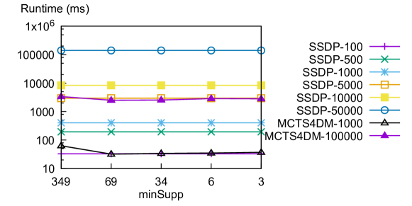
Figure 19: Runtime of SSDP and mcts4dm when varying minSupp in BreastCancer.

Redundancy and diversity in the result set. On one hand, SSDP seems to provide less redundant pattern sets, due to the mutation and cross-over operations of this evolutionary algorithm. Figure 21 (a) deals with the Iris data with $minSupp=7$: The redundancy of SSDP is generally better than those of our algorithm mcts4dm. This is the same conclusion in Figure 20 (b) for Mushroom with $minSupp=56$. On the other hand, the diversity in the result set of SSDP is lower than those of mcts4dm. In Table 9, SSDP fails to extract all hidden patterns in our artificial data. Figure 21 (a) and Figure 21 (b) display the same result for benchmark datasets. Clearly, mcts4dm is able to extract much more interesting subgroups than SSDP. Thus, even if the result set of mcts4dm can be redundant, it provides a more diverse set of patterns compared to the result set extracted by SSDP. This is due to the population size that is not enough large to provide a high diversity (but SSDP is not tractable for large population sizes).

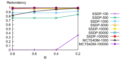
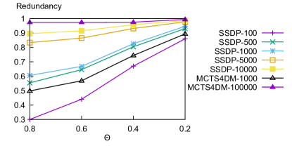
(a) Iris ($minSupp=7$)	(b) Mushroom ($minSupp=56$)

Figure 20: The redundancy in the result set for the iris and mushroom data.

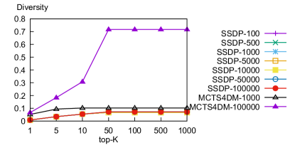
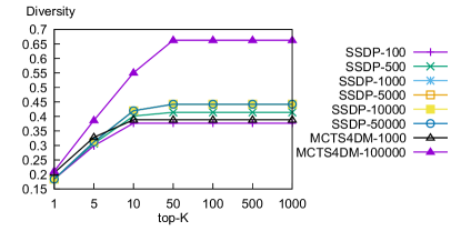
(a) Emotions ($minSupp=5$)	(b) BreastCancer ($minSupp=34$)

Figure 21: The diversity of the result set when $\Theta=0.2$.

Memory consumption. The memory usage of SSDP depends on the size of the population. In mushroom, when considering a population of size $1,000$, the memory usage is higher than those of mcts4dm with $100k$ iterations for high minimum support thresholds but it is lower for low minimum support thresholds (see Figure 15). Indeed, since SSDP does not use any minimum support threshold, its memory usage is independent w.r.t. $minSupp$.

7.4 Sampling approach

Sampling methods are useful to provide interactive applications. Indeed, they enable a result anytime. We experiment with the sampling algorithm Misere [[24, 20, 21]]. Its principle consists in drawing uniformly an object from the data, and then uniformly pick one of its possible generalizations. Each sample is independent and thus a pattern can be drawn several times. We chose Misere as it can consider any pattern quality measure (in contrast to other sampling approaches such as [43, 9]), and it performs very well.

Runtime. Since this strategy consists in randomly drawing patterns, the runtime is linear with the number of draws. Varying the minimum support thresholds does not really impact the runtime (Figure 22). An iteration with mcts4dm is almost only twice much longer than a draw with Misere. This is explained by the fact that Misere only draws one pattern at once without additional memory (i.e., the Monte Carlo tree). Conversely, in one iteration, MCTS additionally performs Select, Expand, Memory and Update steps.

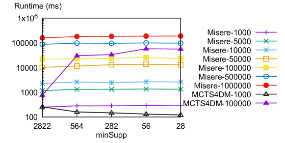
Figure 22: Runtime of Misere and mcts4dm when varying minSupp on the Mushroom dataset.

Redundancy and diversity in the result set. Since Misere proceeds in independent draws of patterns without exploiting the result of the previous draws of patterns, it leads to a result set that contains little redundancy. Indeed, it can draw an interesting pattern that is close to its local optimum, but it would not try to find this optimum at the next draws. Figure 23 illustrates this: The result set is much less redundant than those of mcts4dm. For example, considering a result set containing $1,000$ draws of patterns and another obtained with $1,000$ iterations from mcts4dm. mcts4dm returns pattern set 10 times more redundant than Misere. However, since Misere does not exploit the result of the previous draws, it leads to less diversity. In Table 9, Misere may require lots of draws to find all local optima. Figure 23 (b) shows for Bibtex that the diversity is better with mcts4dm than with Misere. Contrary to mcts4dm, there is no guarantee that Misere will explore the whole search space, even given a large computational budget. Nevertheless, in Table 9, we can notice that, in practice, Misere can extract all patterns hidden in artificial data, but it might require a lot of draws to find them.

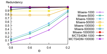
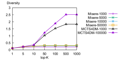
(a) Redundancy in Cal500	(b) Diversity in Bibtex

Figure 23: The redundancy and the diversity in the result set for the Cal500 and Bibtex data.

Memory consumption. As expected, since this sampling method performs independent draws, the memory usage is low. In our settings, only the patterns that are drawn are stored. Figure 15 illustrates the memory usage of Misere when it has randomly picked $100k$ patterns. It is constant w.r.t. the minimum support thresholds, and this is the exploration method that requires the less memory for low minimum support thresholds.

7.5 Considering several measures

mcts4dm can consider any pattern quality measures. Up to now, we experimented with the popular WRAcc measure only. We empirically evaluate mcts4dm with several quality measures that are also used in SD. We consider some of the quality measures available in Cortana: The entropy, the F1 score, the Jaccard coefficient and the accuracy (or precision). The measures we use are not equivalent since they do not sort the patterns in the same order : Each measure induces a specific profile on the pattern space.

mcts4dm is not measure-dependent since it does not use any prior knowledge to explore the search space. During the first iterations, mcts4dm randomly samples the search space, then once it has an estimation – that is usually rather not reliable at the beginning – of the distribution of the quality measure on the pattern space, it biases the exploration to focus on the promising areas (exploitation) and the areas that have been rarely visited (exploration). The strategies we developed are useful to handle the specific profile induced by a quality measure on the pattern space, e.g., if there are lots of local optima in the search space the exploration strategy should be different than if there are few local optima. For instance, the mean-update strategy is the most efficient strategy when we are facing a pattern space with lots of local optima since it enables to exploit the areas that are deemed to be interesting in average. Thus, mcts4dm can be used with any quality measure. The choice of the strategies only impacts how fast it will find the interesting patterns.

We compare our approach with the sampling method Misere which is the most efficient opponent based on the previous results (see Figure 24). We experiment on the Mushroom dataset to reach low minimum support thresholds using the four quality measures (the entropy, the F1 score, the Jaccard coefficient and the accuracy). The results suggest that mcts4dm is able to provide a good diversity regardless the quality measure that is used. mcts4dm finds a result set with a better diversity for all quality measures. The results on the other datasets are similar but not reported here.

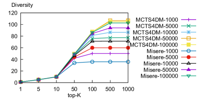
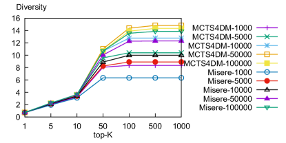
(a) Entropy	(b) F1
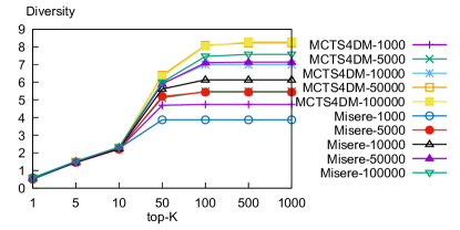
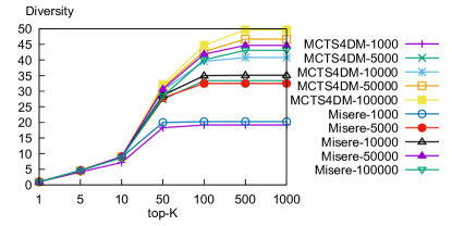
(c) Jaccard coefficient	(d) Accuracy

Figure 24: The diversity of the result set for several quality measures in the Mushroom dataset.

8 Discussion

Based on the empirical study reported in the two previous sections, we now provide a summary of the main results. First, we experimented with several strategies we defined for our algorithm mcts4dm. Our conclusions are the following:

• Select: Concerning the choice of the upper confidence bound, it seems more suitable to use the SP-MCTS for SD problems, although it has a limited impact. Activating LO leads to worse results, but with PU we are able to get more interesting patterns. This is a quite interesting fact as LO is a widely used technique in pattern mining (enumerate each pattern only once with a lectic order).

• Expand: We advise to use the label-gen strategy that enables to reach more quickly the best patterns, but it can require more computational time.

• RollOut: For nominal attributes, the direct-freq-roll-out is an efficient strategy. However, when facing numerical attributes, we recommend to employ the large-freq-roll-out since it may require a lot of time to reach the maximal frequent patterns.

• Memory: Using a memory strategy is essential since it enables to store the patterns encountered during the RollOut step. The top-1-memory is enough to avoid to miss interesting patterns that are located deeper in the search space.

• Update: When there are potentially many local optima in the search space, we recommend to set the mean-update strategy for the Update step. Indeed it enables to exploit the areas that are deemed to be interesting in average. However, when there are few local optima among lots of uninteresting patterns, using mean-update is not optimal since the mean of the rewards would converge to 0. In place, the max-update should be used to ensure that an area containing a local optima is well identified.

Our second batch of experiments compared mcts4dm with the main existing approaches for SD. For that, we experimented with one of the most efficient exhaustive search in SD, namely SD-Map*, a beam search, the recent evolutionary algorithm SSDP and a sampling method implemented in the algorithm Misere. The results suggest that mcts4dm leads, in general, to a more diverse result set when an exhaustive search is not tractable. The greedy property of the beam search leads to a low diversity in the result set, and the lack of memory in sampling methods avoid to exploit interesting patterns to find the local optima (a pattern may be drawn several times). There is no guarantee that evolutionary algorithms and sampling approaches converge to the optimal pattern set even with an infinite computational budget.

MCTS comes with several advantages but has some limits:

• It produces a good pattern set anytime and it converges to an exhaustive search if given enough time and memory (a best-first search).

• It is agnostic of the pattern language and the quality measures: It handles numerical patterns without discretization in a pre-processing step and it still provides a high diversity using several quality measures.

• mcts4dm is aheuristic: No hypotheses are required to run the algorithm whereas with some sampling methods, a probability distribution (based on the quality measure and the pattern space) has to be given as a parameter.

• mcts4dm may require a lot of memory. This memory usage becomes more and more important with the increase of the number of iterations.

• Despite the use of UCB, it is now well known that MCTS algorithms explore too much the search space. As MCTS basically requires to expand all the children of a node before exploiting one of them, this problem is even stronger when dealing with very high branching factor (number of direct specializations of a pattern). This problem has been in part tackled by the progressive widening approach that enables to exploit a child of a node before all of the other children of the node have been expanded [[23, 13]].

9 Conclusion

Heuristic search of supervised patterns becomes mandatory with large datasets. However, classical heuristics lead to a weak diversity in pattern sets: Only few local optima are found. We advocate for the use of MCTS for pattern mining: An exploration strategy leading to “any-time” pattern mining that can be adapted with different measures and policies. The experiments show that MCTS provides a much better diversity in the result set than existing heuristic approaches. For instance, interesting subgroups are found by means of a reasonable amount of iterations and the quality of the result iteratively improves.

MCTS is a powerful exploration strategy that can be applied to several, if not all, pattern mining problems that need to optimize a quality measure given a subset of objects. For example, [6] have already tuned MCTS4DM for mining convex polygon patterns in numerical data. In general, the main difficulties are to be able to deal with large branching factors, and jointly deal with several quality measures. This opens new research perspectives for mining more complex patterns such as sequences and graphs.

References

- [1] Bruce Abramson. Expected-outcome: A general model of static evaluation. IEEE Trans. Pattern Anal. Mach. Intell., 12(2):182–193, 1990.
- [2] Tarek Abudawood and Peter A. Flach. Evaluation measures for multi-class subgroup discovery. In Wray L. Buntine, Marko Grobelnik, Dunja Mladenic, and John Shawe-Taylor, editors, Machine Learning and Knowledge Discovery in Databases, European Conference, ECML PKDD 2009, Bled, Slovenia, September 7-11, 2009, Proceedings, Part I, volume 5781 of Lecture Notes in Computer Science, pages 35–50. Springer, 2009.
- [3] Martin Atzmüller and Florian Lemmerich. Fast subgroup discovery for continuous target concepts. In Jan Rauch, Zbigniew W. Ras, Petr Berka, and Tapio Elomaa, editors, Foundations of Intelligent Systems, 18th International Symposium, ISMIS 2009, Prague, Czech Republic, September 14-17, 2009. Proceedings, volume 5722 of Lecture Notes in Computer Science, pages 35–44. Springer, 2009.
- [4] Martin Atzmüller and Frank Puppe. Sd-map - A fast algorithm for exhaustive subgroup discovery. In Johannes Fürnkranz, Tobias Scheffer, and Myra Spiliopoulou, editors, Knowledge Discovery in Databases: PKDD 2006, 10th European Conference on Principles and Practice of Knowledge Discovery in Databases, Berlin, Germany, September 18-22, 2006, Proceedings, volume 4213 of Lecture Notes in Computer Science, pages 6–17. Springer, 2006.
- [5] Peter Auer, Nicolò Cesa-Bianchi, and Paul Fischer. Finite-time analysis of the multiarmed bandit problem. Machine Learning, 47(2-3):235–256, 2002.
- [6] Aimene Belfodil, Sergei O. Kuznetsov, Céline Robardet, and Mehdi Kaytoue. Mining convex polygon patterns with formal concept analysis. In Carles Sierra, editor, Proceedings of the Twenty-Sixth International Joint Conference on Artificial Intelligence, IJCAI 2017, Melbourne, Australia, August 19-25, 2017, pages 1425–1432. ijcai.org, 2017.
- [7] Ahmed Anes Bendimerad, Marc Plantevit, and Céline Robardet. Unsupervised exceptional attributed sub-graph mining in urban data. In Francesco Bonchi, Josep Domingo-Ferrer, Ricardo A. Baeza-Yates, Zhi-Hua Zhou, and Xindong Wu, editors, IEEE 16th International Conference on Data Mining, ICDM 2016, December 12-15, 2016, Barcelona, Spain, pages 21–30. IEEE, 2016.
- [8] Yngvi Björnsson and Hilmar Finnsson. Cadiaplayer: A simulation-based general game player. IEEE Trans. Comput. Intellig. and AI in Games, 1(1):4–15, 2009.
- [9] Mario Boley, Claudio Lucchese, Daniel Paurat, and Thomas Gärtner. Direct local pattern sampling by efficient two-step random procedures. In Chid Apté, Joydeep Ghosh, and Padhraic Smyth, editors, Proceedings of the 17th ACM SIGKDD International Conference on Knowledge Discovery and Data Mining, San Diego, CA, USA, August 21-24, 2011, pages 582–590. ACM, 2011.
- [10] Guillaume Bosc, Jérôme Golebiowski, Moustafa Bensafi, Céline Robardet, Marc Plantevit, Jean-François Boulicaut, and Mehdi Kaytoue. Local subgroup discovery for eliciting and understanding new structure-odor relationships. In Toon Calders, Michelangelo Ceci, and Donato Malerba, editors, Discovery Science - 19th International Conference, DS 2016, Bari, Italy, October 19-21, 2016, Proceedings, volume 9956 of Lecture Notes in Computer Science, pages 19–34, 2016.
- [11] Jean-François Boulicaut and Baptiste Jeudy. Constraint-based data mining. In Oded Maimon and Lior Rokach, editors, Data Mining and Knowledge Discovery Handbook, 2nd ed., pages 339–354. Springer, 2010.
- [12] Björn Bringmann and Albrecht Zimmermann. One in a million: picking the right patterns. Knowl. Inf. Syst., 18(1):61–81, 2009.
- [13] Cameron Browne, Edward Jack Powley, Daniel Whitehouse, Simon M. Lucas, Peter I. Cowling, Philipp Rohlfshagen, Stephen Tavener, Diego Perez Liebana, Spyridon Samothrakis, and Simon Colton. A survey of monte carlo tree search methods. IEEE Trans. Comput. Intellig. and AI in Games, 4(1):1–43, 2012.
- [14] Cristóbal J. Carmona, Pedro González, María José del Jesús, and Francisco Herrera. NMEEF-SD: non-dominated multiobjective evolutionary algorithm for extracting fuzzy rules in subgroup discovery. IEEE Trans. Fuzzy Systems, 18(5):958–970, 2010.
- [15] María José del Jesús, Pedro González, Francisco Herrera, and Mikel Mesonero. Evolutionary fuzzy rule induction process for subgroup discovery: A case study in marketing. IEEE Trans. Fuzzy Systems, 15(4):578–592, 2007.
- [16] Lennart Downar and Wouter Duivesteijn. Exceptionally monotone models - the rank correlation model class for exceptional model mining. Knowl. Inf. Syst., 51(2):369–394, 2017.
- [17] Wouter Duivesteijn, Ad Feelders, and Arno J. Knobbe. Exceptional model mining - supervised descriptive local pattern mining with complex target concepts. Data Min. Knowl. Discov., 30(1):47–98, 2016.
- [18] Wouter Duivesteijn and Arno J. Knobbe. Exploiting false discoveries - statistical validation of patterns and quality measures in subgroup discovery. In Diane J. Cook, Jian Pei, Wei Wang, Osmar R. Zaïane, and Xindong Wu, editors, 11th IEEE International Conference on Data Mining, ICDM 2011, Vancouver, BC, Canada, December 11-14, 2011, pages 151–160. IEEE Computer Society, 2011.
- [19] Wouter Duivesteijn, Arno J. Knobbe, Ad Feelders, and Matthijs van Leeuwen. Subgroup discovery meets bayesian networks – an exceptional model mining approach. In Geoffrey I. Webb, Bing Liu, Chengqi Zhang, Dimitrios Gunopulos, and Xindong Wu, editors, ICDM 2010, The 10th IEEE International Conference on Data Mining, Sydney, Australia, 14-17 December 2010, pages 158–167. IEEE Computer Society, 2010.
- [20] Elias Egho, Dominique Gay, Marc Boullé, Nicolas Voisine, and Fabrice Clérot. A parameter-free approach for mining robust sequential classification rules. In Charu C. Aggarwal, Zhi-Hua Zhou, Alexander Tuzhilin, Hui Xiong, and Xindong Wu, editors, 2015 IEEE International Conference on Data Mining, ICDM 2015, Atlantic City, NJ, USA, November 14-17, 2015, pages 745–750. IEEE Computer Society, 2015.
- [21] Elias Egho, Dominique Gay, Marc Boullé, Nicolas Voisine, and Fabrice Clérot. A user parameter-free approach for mining robust sequential classification rules. Knowl. Inf. Syst., 52(1):53–81, 2017.
- [22] Johannes Fürnkranz, Dragan Gamberger, and Nada Lavrac. Foundations of Rule Learning. Cognitive Technologies. Springer, 2012.
- [23] Romaric Gaudel and Michèle Sebag. Feature selection as a one-player game. In Johannes Fürnkranz and Thorsten Joachims, editors, Proceedings of the 27th International Conference on Machine Learning (ICML-10), June 21-24, 2010, Haifa, Israel, pages 359–366. Omnipress, 2010.
- [24] Dominique Gay and Marc Boullé. A bayesian approach for classification rule mining in quantitative databases. In Peter A. Flach, Tijl De Bie, and Nello Cristianini, editors, Machine Learning and Knowledge Discovery in Databases - European Conference, ECML PKDD 2012, Bristol, UK, September 24-28, 2012. Proceedings, Part II, volume 7524 of Lecture Notes in Computer Science, pages 243–259. Springer, 2012.
- [25] Sylvain Gelly and David Silver. Combining online and offline knowledge in UCT. In Zoubin Ghahramani, editor, Machine Learning, Proceedings of the Twenty-Fourth International Conference (ICML 2007), Corvallis, Oregon, USA, June 20-24, 2007, volume 227 of ACM International Conference Proceeding Series, pages 273–280. ACM, 2007.
- [26] Henrik Grosskreutz, Stefan Rüping, and Stefan Wrobel. Tight optimistic estimates for fast subgroup discovery. In Walter Daelemans, Bart Goethals, and Katharina Morik, editors, Machine Learning and Knowledge Discovery in Databases, European Conference, ECML/PKDD 2008, Antwerp, Belgium, September 15-19, 2008, Proceedings, Part I, volume 5211 of Lecture Notes in Computer Science, pages 440–456. Springer, 2008.
- [27] Jiawei Han, Jian Pei, and Yiwen Yin. Mining frequent patterns without candidate generation. In Weidong Chen, Jeffrey F. Naughton, and Philip A. Bernstein, editors, Proceedings of the 2000 ACM SIGMOD International Conference on Management of Data, May 16-18, 2000, Dallas, Texas, USA., pages 1–12. ACM, 2000.
- [28] Jiawei Han, Jian Pei, Yiwen Yin, and Runying Mao. Mining frequent patterns without candidate generation: A frequent-pattern tree approach. Data Min. Knowl. Discov., 8(1):53–87, 2004.
- [29] David P. Helmbold and Aleatha Parker-Wood. All-moves-as-first heuristics in monte-carlo go. In Hamid R. Arabnia, David de la Fuente, and José Angel Olivas, editors, Proceedings of the 2009 International Conference on Artificial Intelligence, ICAI 2009, July 13-16, 2009, Las Vegas Nevada, USA, 2 Volumes, pages 605–610. CSREA Press, 2009.
- [30] J. H. Holland. Adaptation in natural and artificial systems: an introductory analysis with applications to biology, control, and artificial intelligence. U Michigan Press, 1975.
- [31] Branko Kavsek and Nada Lavrac. APRIORI-SD: adapting association rule learning to subgroup discovery. Applied Artificial Intelligence, 20(7):543–583, 2006.
- [32] Mehdi Kaytoue, Sergei O. Kuznetsov, and Amedeo Napoli. Revisiting numerical pattern mining with formal concept analysis. In Toby Walsh, editor, IJCAI 2011, Proceedings of the 22nd International Joint Conference on Artificial Intelligence, Barcelona, Catalonia, Spain, July 16-22, 2011, pages 1342–1347. IJCAI/AAAI, 2011.
- [33] Mehdi Kaytoue, Marc Plantevit, Albrecht Zimmermann, Ahmed Anes Bendimerad, and Céline Robardet. Exceptional contextual subgraph mining. Machine Learning, 106(8):1171–1211, 2017.
- [34] Willi Klösgen. Explora: A multipattern and multistrategy discovery assistant. In Advances in Knowledge Discovery and Data Mining, pages 249–271. AAAI/MIT Press, 1996.
- [35] Levente Kocsis and Csaba Szepesvári. Bandit based monte-carlo planning. In Johannes Fürnkranz, Tobias Scheffer, and Myra Spiliopoulou, editors, Machine Learning: ECML 2006, 17th European Conference on Machine Learning, Berlin, Germany, September 18-22, 2006, Proceedings, volume 4212 of Lecture Notes in Computer Science, pages 282–293. Springer, 2006.
- [36] Nada Lavrac, Bojan Cestnik, Dragan Gamberger, and Peter A. Flach. Decision support through subgroup discovery: Three case studies and the lessons learned. Machine Learning, 57(1-2):115–143, 2004.
- [37] Nada Lavrac, Peter A. Flach, and Blaz Zupan. Rule evaluation measures: A unifying view. In Saso Dzeroski and Peter A. Flach, editors, Inductive Logic Programming, 9th International Workshop, ILP-99, Bled, Slovenia, June 24-27, 1999, Proceedings, volume 1634 of Lecture Notes in Computer Science, pages 174–185. Springer, 1999.
- [38] Dennis Leman, Ad Feelders, and Arno J. Knobbe. Exceptional model mining. In Walter Daelemans, Bart Goethals, and Katharina Morik, editors, Machine Learning and Knowledge Discovery in Databases, European Conference, ECML/PKDD 2008, Antwerp, Belgium, September 15-19, 2008, Proceedings, Part II, volume 5212 of Lecture Notes in Computer Science, pages 1–16. Springer, 2008.
- [39] Florian Lemmerich, Martin Atzmueller, and Frank Puppe. Fast exhaustive subgroup discovery with numerical target concepts. Data Min. Knowl. Discov., 30(3):711–762, 2016.
- [40] B. T. Lowerre. The HARPY speech recognition system. PhD thesis, Carnegie-Mellon Univ., Pittsburgh, PA. Dept. of Computer Science., 1976.
- [41] Tarcísio Lucas, Túlio C. P. B. Silva, Renato Vimieiro, and Teresa Bernarda Ludermir. A new evolutionary algorithm for mining top-k discriminative patterns in high dimensional data. Appl. Soft Comput., 59:487–499, 2017.
- [42] Marvin Meeng, Wouter Duivesteijn, and Arno J. Knobbe. Rocsearch - an roc-guided search strategy for subgroup discovery. In Mohammed Javeed Zaki, Zoran Obradovic, Pang-Ning Tan, Arindam Banerjee, Chandrika Kamath, and Srinivasan Parthasarathy, editors, Proceedings of the 2014 SIAM International Conference on Data Mining, Philadelphia, Pennsylvania, USA, April 24-26, 2014, pages 704–712. SIAM, 2014.
- [43] Sandy Moens and Mario Boley. Instant exceptional model mining using weighted controlled pattern sampling. In Hendrik Blockeel, Matthijs van Leeuwen, and Veronica Vinciotti, editors, Advances in Intelligent Data Analysis XIII - 13th International Symposium, IDA 2014, Leuven, Belgium, October 30 - November 1, 2014. Proceedings, volume 8819 of Lecture Notes in Computer Science, pages 203–214. Springer, 2014.
- [44] Marianne Mueller, Rómer Rosales, Harald Steck, Sriram Krishnan, Bharat Rao, and Stefan Kramer. Subgroup discovery for test selection: A novel approach and its application to breast cancer diagnosis. In Niall M. Adams, Céline Robardet, Arno Siebes, and Jean-François Boulicaut, editors, Advances in Intelligent Data Analysis VIII, 8th International Symposium on Intelligent Data Analysis, IDA 2009, Lyon, France, August 31 - September 2, 2009. Proceedings, volume 5772 of Lecture Notes in Computer Science, pages 119–130. Springer, 2009.
- [45] Petra Kralj Novak, Nada Lavrac, and Geoffrey I. Webb. Supervised descriptive rule discovery: A unifying survey of contrast set, emerging pattern and subgroup mining. Journal of Machine Learning Research, 10:377–403, 2009.
- [46] Victoria Pachón, Jacinto Mata Vázquez, Juan Luis Domínguez, and Manuel J. Maña López. Multi-objective evolutionary approach for subgroup discovery. In Emilio Corchado, Marek Kurzynski, and Michal Wozniak, editors, Hybrid Artificial Intelligent Systems - 6th International Conference, HAIS 2011, Wroclaw, Poland, May 23-25, 2011, Proceedings, Part II, volume 6679 of Lecture Notes in Computer Science, pages 271–278. Springer, 2011.
- [47] Daniel Rodríguez, Roberto Ruiz, José C. Riquelme, and Jesús S. Aguilar-Ruiz. Searching for rules to detect defective modules: A subgroup discovery approach. Inf. Sci., 191:14–30, 2012.
- [48] Stuart J. Russell and Peter Norvig. Artificial Intelligence - A Modern Approach (3. internat. ed.). Pearson Education, 2010.
- [49] Maarten P. D. Schadd, Mark H. M. Winands, H. Jaap van den Herik, Guillaume Chaslot, and Jos W. H. M. Uiterwijk. Single-player monte-carlo tree search. In H. Jaap van den Herik, Xinhe Xu, Zongmin Ma, and Mark H. M. Winands, editors, Computers and Games, 6th International Conference, CG 2008, Beijing, China, September 29 - October 1, 2008. Proceedings, volume 5131 of Lecture Notes in Computer Science, pages 1–12. Springer, 2008.
- [50] D. Silver, A. Huang, C. J. Maddison, A. Guez, L. Sifre, G. van den Driessche, J. Schrittwieser, I. Antonoglou, V. Panneershelvam, M. Lanctot, S. Dieleman, D. Grewe, J. Nham, N. Kalchbrenner, I. Sutskever, T. P. Lillicrap, M. Leach, K. Kavukcuoglu, T. Graepel, and D. Hassabis. Mastering the game of go with deep neural networks and tree search. Nature, 529(7587):484–489, 2016.
- [51] Matthijs van Leeuwen and Esther Galbrun. Association discovery in two-view data. IEEE Trans. Knowl. Data Eng., 27(12):3190–3202, 2015.
- [52] Matthijs van Leeuwen and Arno J. Knobbe. Non-redundant subgroup discovery in large and complex data. In Dimitrios Gunopulos, Thomas Hofmann, Donato Malerba, and Michalis Vazirgiannis, editors, Machine Learning and Knowledge Discovery in Databases - European Conference, ECML PKDD 2011, Athens, Greece, September 5-9, 2011, Proceedings, Part III, volume 6913 of Lecture Notes in Computer Science, pages 459–474. Springer, 2011.
- [53] Matthijs van Leeuwen and Arno J. Knobbe. Diverse subgroup set discovery. Data Min. Knowl. Discov., 25(2):208–242, 2012.
- [54] Matthijs van Leeuwen and Antti Ukkonen. Discovering skylines of subgroup sets. In Hendrik Blockeel, Kristian Kersting, Siegfried Nijssen, and Filip Zelezný, editors, Machine Learning and Knowledge Discovery in Databases - European Conference, ECML PKDD 2013, Prague, Czech Republic, September 23-27, 2013, Proceedings, Part III, volume 8190 of Lecture Notes in Computer Science, pages 272–287. Springer, 2013.
- [55] Stefan Wrobel. An algorithm for multi-relational discovery of subgroups. In Henryk Jan Komorowski and Jan M. Zytkow, editors, Principles of Data Mining and Knowledge Discovery, First European Symposium, PKDD ’97, Trondheim, Norway, June 24-27, 1997, Proceedings, volume 1263 of Lecture Notes in Computer Science, pages 78–87. Springer, 1997.