The puzzling properties of the magnetic O star Tr16-22

Abstract

Context. The detection of bright, hard, and variable X-ray emission in Tr16-22 prompted spectropolarimetric observations of this star, which in turn led to the discovery of a surface magnetic field.

Aims. We want to further constrain the properties of this star, in particular to verify whether X-ray variations are correlated to changes in optical emission lines and magnetic field strength, as expected from the oblique rotator model that is widely accepted for magnetic O stars.

Methods. We have obtained new low-resolution spectropolarimetric and long-term high-resolution spectroscopic monitoring of Tr16-22, and we also analyse new, serendipitous X-ray data.

Results. The new X-ray observations are consistent with previous data, but their addition does not help to solve the ambiguity in the variation timescale because of numerous aliases. No obvious periodicity or any large variations are detected in the spectropolarimetric data of Tr16-22 obtained over three months. The derived field values appear to be in line with previous measurements, suggesting constancy of the field (though the possibility of small, short-term field variations cannot be excluded). Variations in the equivalent widths of H$\alpha$ are very small, and they do not appear to be related to the X-ray timescale; the overall lack of large variations in optical emission lines is consistent with the magnetic field constancy. In addition, variations of the radial velocities indicate that Tr16-22 is probably a SB1 binary with a very long period.

Conclusions. Our new measurements of optical emission lines and magnetic field strength do not show an obvious correlation with X-ray variations. Our current data thus cannot be interpreted in terms of the common model, which assumes the electromagnetic emission associated with a wind confined by a dipolar field tilted with respect to the rotation axis. However, the sampling is imperfect and new data are needed to further constrain the actual periodicity of the various observed phenomena. If inconsistencies are confirmed, then we will need to consider alternative scenarios.

1 Introduction

Strong magnetic fields have been detected in a dozen O stars during the last decade (Petit et al., 2013; Fossati et al., 2015, and references therein). In such objects, the stellar wind flows are channelled towards the equator (Babel & Montmerle, 1997a), creating a dense region of confined winds. Part of this material is shock-heated to higher temperatures, leading to the emission of X-rays, while the cooler plasma is easily detected in the visible (e.g. through Balmer emission lines). When the rotation axis is not perfectly aligned with the magnetic axis, a periodic modulation of the electromagnetic emission associated with these confined winds is observed. Variations of the longitudinal field, of the broad-band photometry, of the visible emission lines, and of the X-ray flux thus occur simultaneously, as was found for example for $\theta^{1}$ Ori C (Donati et al., 2002; Gagné et al., 2005) or HD 191612 (Donati et al., 2006; Nazé et al., 2007; Howarth et al., 2007; Nazé et al., 2010).

Table 1: List of the new X-ray observations. Phases were calculated considering $1/P$=0.01838 d^-1 and $T_{0}$ as the date of the oldest XMM-Newton observation (No. 4 in Table 1 of Nazé et al. 2014a, $JD$=2 451 751.707).

ObsID	exp.	Start Date	Associated JD	$\phi$
	time
0691970101	87 ks	2012-Dec-20@19:21:54	2456282.307	0.27
0742850301	13 ks	2014-Jun-06@19:13:05	2456815.301	0.07
0742850401	33 ks	2014-Jul-28@15:32:43	2456867.148	0.02
0762910401	11 ks	2015-Jul-16@01:18:44	2457219.555	0.50

Spectropolarimetric observations found Tr16-22 (O8.5V) to be strongly magnetic (Nazé et al., 2012, 2014a). In the X-ray range, Tr16-22 displays a bright, variable, and hard emission atypical of single, “normal” massive stars (Evans et al., 2004; Antokhin et al., 2008; Nazé et al., 2011, 2014a), but in line with theoretical expectations for confined winds (Nazé et al., 2014b). The Fourier analysis of the X-ray data clearly indicated the presence of a periodicity; the favoured value was $\sim$54d but many aliases were present, leaving some ambiguity on the actual period (Nazé et al., 2014a). Therefore, to better constrain its physical properties, we needed additional data of Tr16-22.

In this paper, we analyse these new data. Section 2 presents the observations used in the study, Sect. 3 provides the results, and Sect. 4 reports our conclusions.

2 Observations

2.1 X-ray observations

Being close to $\eta$ Carinae, Tr16-22 is frequently observed at high energies. Since the observations presented in Nazé et al. (2014a), three new XMM-Newton exposures are available in the archives and an additional one was kindly provided by Dr Kenji Hamaguchi (Table 1). In these observations, the target only appears on the MOS2 camera: it falls outside the field of view of the other two cameras (because of dead CCDs in MOS1 or the use of the small window mode in MOS1 or pn). These new data were reduced with SAS v14.0.0 using calibration files available in December 2015 and following the recommendations of the XMM-Newton team. Only the best quality data ($PATTERN$ of 0–12) were kept and background flares were discarded. A source detection was performed on each EPIC dataset using the task edetect_chain on the 0.4–10.0 keV energy band and for a likelihood of 10 to find the best-fit position of the target in each dataset. We note that the source is not bright enough to present pile-up. EPIC spectra were extracted using the task especget for circular regions of 35” radius centred on these best-fit positions and, for the backgrounds, at positions as close as possible to the target considering crowding and CCD edges. The spectra were finally grouped, using specgroup, to obtain an oversampling factor of five and to ensure that a minimum signal-to-noise ratio of three (i.e. a minimum of 10 counts) was reached in each spectral bin of the background-corrected spectra.

The X-ray spectra were then fitted within Xspec v12.7.0 using the same models as in Nazé et al. (2014a), i.e. absorbed optically thin thermal plasma models, i.e. $wabs\times phabs\times\sum apec$, with solar abundances (Anders & Grevesse, 1989). The first absorption component is the interstellar column, fixed to $4.4\times 10^{21}$ cm^-2 (a value calculated using the colour excess of the star and the conversion formula $5.8\times 10^{21}\times E(B-V)$ cm^-2 from Bohlin et al. 1978), while the second absorption represents additional (local) absorption. For the emission components, we considered either two or four temperatures, as in Nazé et al. (2014a). Table 2 yields the results of our X-ray fittings. Since the 2012 December exposure is long, we also extracted the X-ray lightcurve of Tr16-22 using the same regions as for spectrum extraction. Dedicated $\chi^{2}$ tests were then performed and did not reveal any significant variability of Tr16-22 during this observation.

Table 2: Results from the X-ray spectral fitting.

A. Model $wabs\times phabs\times(apec+apec)$
ID	$norm_{1}$	$norm_{2}$	$\chi^{2}$(dof)	$F_{\rm X}^{obs}$	$L_{\rm X}^{ISMcor}$	$HR$
	(cm-5)			erg cm-2 s-1	erg s-1
0691970101	1.45$\pm$0.18e-3	3.43$\pm$0.22e-4	0.92 (46)	2.58$\pm$0.10e-13	1.78e32	0.52$\pm$0.04
0742850301	1.07$\pm$0.39e-3	2.91$\pm$0.43e-4	0.40 (9)	2.12$\pm$0.20e-13	1.39e32	0.56$\pm$0.11
0742850401	1.09$\pm$0.23e-3	2.77$\pm$0.26e-4	0.91 (26)	2.05$\pm$0.13e-13	1.37e32	0.54$\pm$0.07
0762910401	1.53$\pm$0.43e-3	3.06$\pm$0.50e-4	0.61 (9)	2.40$\pm$0.25e-13	1.78e32	0.47$\pm$0.10
B. Model $wabs\times phabs\times\sum_{4}apec$
ID	$norm_{1}$	$norm_{3}$	$norm_{4}$	$\chi^{2}$(dof)	$F_{\rm X}^{obs}$	$L_{\rm X}^{ISMcor}$	$HR$
	(cm-5)				erg cm-2 s-1	erg s-1
0691970101	2.44$\pm$0.97e-3	3.63$\pm$0.47e-4	1.04$\pm$0.25e-4	0.87 (45)	2.71$\pm$0.21e-13	1.71e32	0.58$\pm$0.07
0742850301	1.51$\pm$2.11e-3	3.03$\pm$1.08e-4	9.13$\pm$5.32e-5	0.40 (8)	2.24$\pm$0.37e-13	1.31e32	0.65$\pm$0.22
0742850401	2.90$\pm$1.25e-3	2.18$\pm$0.60e-4	1.26$\pm$0.27e-4	0.70 (25)	2.42$\pm$0.20e-13	1.44e32	0.67$\pm$0.11
0762910401	3.28$\pm$2.31e-3	3.06$\pm$1.15e-4	1.04$\pm$0.51e-4	0.82 (8)	2.57$\pm$0.36e-13	1.74e32	0.53$\pm$0.15

For the model $wabs\times phabs\times(apec+apec)$, absorptions were fixed to $4.4\times 10^{21}$ cm^-2 and $6.3\times 10^{21}$ cm^-2, and temperatures to 0.28 keV and 1.78 keV (as in Nazé et al. 2014a, Table 2). For the model $wabs\times phabs\times\sum_{4}apec$ (used for the general spectral fits in the X-ray survey of magnetic stars performed by Nazé et al. 2014b), absorptions were fixed to $4.4\times 10^{21}$ cm^-2 and $7.0\times 10^{21}$ cm^-2, and temperatures to 0.2, 0.6, 1.0, and 4.0 keV, while $norm_{2}$ was kept to zero (as in Nazé et al. 2014a, Table 3). The remaining free parameters, the strengths of the thermal components, are listed above with their $1\sigma$ errors, the goodness of fit, and the number of degrees of freedom. The last columns provide the observed fluxes and ISM-absorption corrected luminosities (both in the 0.5–10. keV range and for a distance of 2290 pc), as well as the ratio ($HR$) between the hard (2.–10.0 keV) and soft (0.5–2.0 keV) ISM absorption-corrected fluxes.

2.2 Spectropolarimetry

Spectropolarimetric data of Tr16-22 had been obtained with the Very Large Telescope equipped with FORS2 in 2011 (Nazé et al., 2012) and 2013 (Nazé et al., 2014a). In view of the variations detected in X-rays, we requested a monitoring of the star (Prog. 095.D-0082, PI Nazé): seven additional observations were taken in service mode between April and June 2015 (Table 3). These new data were taken with the red CCD (a mosaic composed of two 2k$\times$4k MIT chips) without binning, with a slit of 1” and the 1200B grating ($R\sim 1400$). The observing sequence consisted of 8 subexposures of 240s duration (except for one night, 2015 June 06, where it was pushed up to 500s) with retarder waveplate positions of $+45^{\circ}$, $-45^{\circ}$, $-45^{\circ}$, $+45^{\circ}$, $+45^{\circ}$, $-45^{\circ}$, $-45^{\circ}$, $+45^{\circ}$. We reduced these spectropolarimetric data with IRAF as explained by Nazé et al. (2012): aperture extraction radius fixed to 20 px, subtraction of nearby sky background, and wavelength calibration from 3675 to 5128Å (with pixels of 0.25Å) considering arc lamp data taken at only one retarder waveplate position (in our case $-45^{\circ}$). This allowed us to construct the normalized Stokes $V/I$ profile, as well as a diagnostic “null” profile (Donati et al., 1997; Bagnulo et al., 2009). We note that the signal-to-noise ratio of the derived $I$ spectra near 5000Å was about 1100–1200. Finally, the associated longitudinal magnetic field was estimated by minimizing $\chi^{2}=\sum_{i}\frac{(y_{i}-B_{z}\,x_{i}-a)^{2}}{\sigma^{2}_{i}}$ with $y_{i}$ either $V/I$ or the null profile at the wavelength $\lambda_{i}$ and $x_{i}=-g_{\mathrm{eff}}\ 4.67\times 10^{-13}\ \lambda^{2}_{i}\ 1/I_{i}\ (\mathrm{d}I/\mathrm{d}\lambda)_{i}$ (Bagnulo et al., 2002). This was done for $x_{i}$ in the interval between $-10^{-6}$ to $+10^{-6}$ (an interval where the vast majority of good points are available, avoiding potential problems in slope determination due to a few isolated data points at extreme $x_{i}$, although we note that enlarging the interval, e.g. $\pm 1.6\times 10^{-6}$, does not significantly change the reported values) after discarding edges and deviant points, after rectifying the Stokes profiles, and after selecting spectral windows centred on lines (see Nazé et al., 2012, for further discussion). Table 3 yields the resulting field values, along with the values for the old datasets (recalculated for the same spectral windows).

Table 3: Results from the spectropolarimetry (using rectification and within the same spectral windows). Phases were calculated as in Table 1.

Date	HJD	$\phi$	$B_{z}$ (G)	$N_{z}$ (G)
	–2450000
2011-Mar-12	5632.617	0.33	$-502\pm$77	38$\pm$79
2011-Mar-13	5633.589	0.34	$-662\pm$94	$-89\pm$89
2013-Apr-18	6400.581	0.45	$-479\pm$79	$-87\pm$73
2013-Jul-29	6503.483	0.34	$-543\pm$124	43$\pm$121
2015-Apr-03	7115.616	0.59	$-529\pm$91	132$\pm$91
2015-May-01	7143.590	0.10	$-288\pm$88	$-204\pm$83
2015-May-11	7153.715	0.29	$-189\pm$100	$-264\pm$96
2015-May-19	7161.641	0.43	$-530\pm$95	$-61\pm$93
2015-May-20	7162.626	0.45	$-205\pm$92	$-93\pm$85
2015-Jun-06	7179.545	0.76	$-446\pm$76	23$\pm$69
2015-Jun-18	7191.525	0.98	$-446\pm$115	94$\pm$110

2.3 High-resolution spectroscopy

Data used in this work correspond to spectra collected in three different observatories over a time span of eighteen years. Ten spectra covering 3600–6100Å with a resolving power of 15000 were obtained with the REOSC échelle spectrograph attached to the 2.15m Jorge Sahade telescope at Complejo Astronómico El Leoncito (CASLEO, Argentina), during 1997, 1998, 2011, and 2015. Thirteen spectra covering 3450–9850Å with a resolving power of 40000 were gathered with the échelle spectrograph attached to the 2.5m du Pont telescope at Las Campanas Observatory (LCO, Chile), in 2010, 2013, 2015, and 2016. For these CASLEO and LCO spectra, calibration lamp exposures were secured immediately before or after each star integration at the same sky position. Data were reduced and processed in a standard way using the usual IRAF routines. In addition, two spectra of Tr16-22 were obtained with the FEROS spectrograph attached to the 2.2m telescope at ESO La Silla Observatory (Chile) in 2011 (086.D-0997B) and 2015 (089.D-0975A). These spectra, covering 3570–9210Å with a resolving power of 46000, were gathered following the standard ESO procedures, and they were reduced using the FEROS pipeline provided for MIDAS. We note that spectra obtained after 2010 were taken in the framework of the program “OWN Survey”, a spectroscopic monitoring of southern Galactic O- and WN-type stars (Barbá et al., 2010), while the CASLEO spectra obtained in the nineties are part of the XMEGA project (Corcoran et al., 1999; Albacete Colombo et al., 2001).

3 Results and discussion

In the X-ray range, the new data are in line with previous observations. First, the new data appear amongst the old ones in the flux-hardness relation (see Fig. 1). Second, the periodogram does not change much if the new data are included: $\sim$54 d is still the favoured period and folding with this timescale yields the same, coherent behaviour as shown before (see right panel of Fig. 1 and Nazé et al., 2014a). However, ambiguities on the period remain because aliases are still numerous (typically spaced by $4\times 10^{-4}$ d^-1). As mentioned in Nazé et al. (2014a), the datasets recorded in 2003 provide a hint that the variation timescale may not be very long as the observed flux increased that year by about 30% over two weeks at the end of July and beginning of August, then went back to its level in mid-August. Nevertheless, no full cycle was observed in a single observing run, and only observations with a higher cadence might be able to remove the ambiguity on the periodicity.

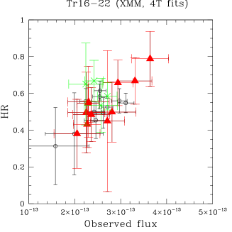
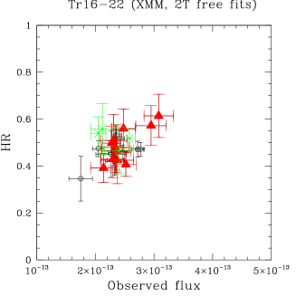
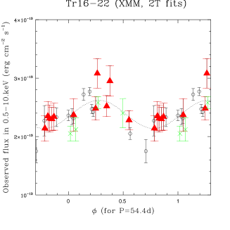
Figure 1: Left and Middle: Evolution of the hardness ratios ($HR=H/S=F^{ISMcor}(2.-10.0\,keV)/F^{ISMcor}(0.5-2.\,keV)$) as a function of observed fluxes. Red triangles correspond to the 2003 XMM-Newton data (the year with the largest number of observations), green crosses to the new data, and black open circles to the other XMM-Newton observations. The values shown in the left (resp. middle) panel correspond to the results from 4T fits (resp. 2T fits). Right: Evolution of the observed fluxes from 2T fits as a function of phase (with $1/P$=0.01838 d^-1 and $T_{0}$=2 451 751.707), along with the best-fit sinusoid (dotted line).

Concerning magnetic field measurements, the 2015 FORS2 data formally provide only three secure detections (i.e. detections at $5-6\sigma$; see Bagnulo et al. 2012). Nevertheless, these new data sample very different phases of the favoured X-ray timescale, allowing it to be tested (see phases in the second column of Table 2). Unfortunately, the longitudinal field values do not show coherent variations when folded with this timescale (see Fig. 2): secure detections and non-detections are both notably found around phase 0.3. The problem remains even when using only the 2015 data, where the precision of the ephemeris has less impact on the folding; for example, only the first of two consecutive days (May 19 and 20) provide a secure detection. Formally, a $\chi^{2}$ test finds a very small chance (0.6%) for the $B_{z}$ values to be constant, but in fact the errors are underestimated – only $5\sigma$ detections are secure with FORS2 spectropolarimetry when $3\sigma$ is usually sufficient (Bagnulo et al., 2012). Indeed, the largest difference between the 2015 values actually only amounts to $\sim$300G, i.e. around $3\sigma$. Therefore, we can conclude that, within the errors, the field has remained constant over the three months of observations, i.e. variations may be possible, but only with a very small amplitude ($<$300G). Furthermore, the 2015 longitudinal field strengths are similar to those based on 2011 or 2013 data, hinting at long-term constancy, though no clear conclusion can be drawn on possibly longer timescales as their sampling is far from perfect. For completeness, we have performed a period search on $B_{z}$ and $N_{z}$ values, but the derived periodograms are similar hence no significant periodicity can be identified for the stellar field measurements. These results appear somewhat at odds with the X-ray variations. In the context of an oblique rotator model, the flux doubling recorded at high energies suggested a high $i+\beta$ value for the dipolar field, with large changes in $B_{z}$ being expected. On the contrary, as large magnetic field variations over tens of days appear excluded by observations, this rather suggests either a pole-on configuration ($i\sim 0$), an alignment of rotational and magnetic axes ($\beta\sim 0$), or a very long rotation period.

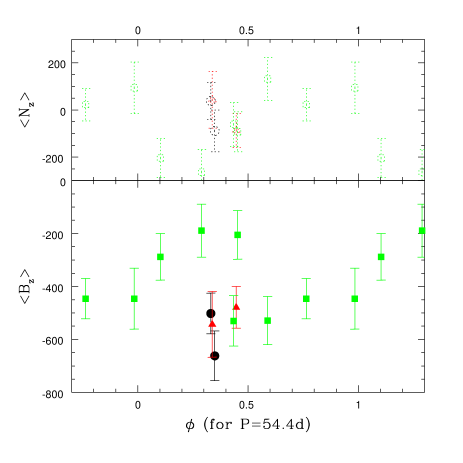
Figure 2: Longitudinal field values (filled symbols) and the associated values for the null profiles (dotted empty symbols) as a function of phase (with $1/P$=0.01838 d^-1 and $T_{0}$=2 451 751.707). The black circles correspond to 2011 data, the red triangles to 2013 data, and the green squares to 2015 data.

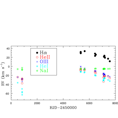
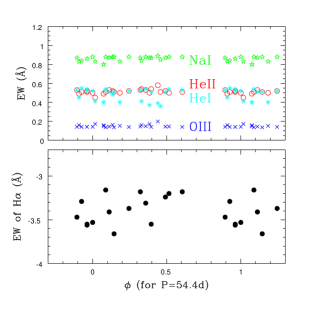
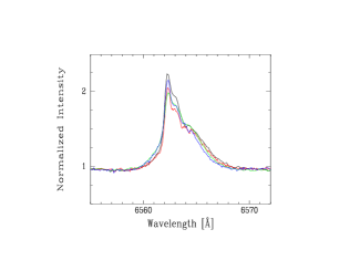
Figure 3: Left and Middle: RVs (left panel) and EWs (middle panel) of selected lines (He ii 4686 shown as open red circles, O iii 5592 as blue crosses, He i 5876 as cyan asterisks, Na i 5890 as green stars, and H$\alpha$ as black dots) as a function of time or phase (with $1/P$=0.01838 d^-1 and $T_{0}$=2 451 751.707), respectively. Typical errors are $<$5 km s^-1 for RVs and $<$10% for EWs (see Table 4). Right: H$\alpha$ profile observed in 2010 (black, $HJD$=2 453 40.538), 2011 (red, $HJD$=2 455 642.689), 2013 (green, $HJD$=2 456 498.481), and 2015 (blue, $HJD$=2 457 116.539).

For the optical spectra, the radial velocities and equivalent widths (EWs, estimated by integrating the line over a fixed interval) were measured for lines of different origins (interstellar, photospheric, circumstellar); the results are provided in Table 4. For H$\alpha$, this was done after the narrow nebular component was subtracted, which could only be done on the high-resolution spectra, but this procedure is imperfect as demonstrated by e.g. residual [O iii] emissions. The radial velocities of all stellar lines yield coherent results (left panel of Fig. 3). In particular, the systematic, coherent trend towards more negative velocities since 2010 (at a rate of $\sim$3.5km s^-1 per year) should be noted. Formally, velocities are significantly variable: they display a larger dispersion than that of the interstellar Na i line ($\sim$7 km s^-1 vs 0.2 km s^-1 in high-resolution data) and the maximum RV difference amount to about 20 km s^-1 corresponding to $\sim 14\sigma$ since typical RV errors on high-resolution spectra are only 1 km s^-1 (i.e. RV variability criterion of Sana et al. 2013 is fulfilled). As no obvious line profile changes are detected, these RV variations indicate that Tr16-22 is a probable SB1 with a long period. To find the binary timescale, we applied the same set of period search algorithms as used before. Unfortunately, no unambiguous periodicity could be pinpointed for the RVs measured on Tr16-22, most probably because of the sparse sampling of the optical data. In view of the measured values, however, long periods ($>>$ tens of days, clearly incompatible with the 54 d putative X-ray period) are favoured, and may be more precisely constrained by further monitoring the system.

While detecting RV variations is an interesting result, our main objective was to study magnetically confined winds, and this is performed through analysing line strengths of circumstellar emissions. It is now well known that Balmer lines, He ii 4686, and He i lines are particularly sensitive indicators of confined winds (see e.g. the case of HD 191612 in Nazé et al., 2007). We found that, for any given line (interstellar, stellar, or circumstellar), the EWs always remain similar, with a small dispersion ($<$0.01Å on high-resolution data). Only the H$\alpha$ line displays some significant variations, and Fourier analyses tentatively yield a best period of about 8 d for them. However, aliases are numerous and the current sampling of high-resolution spectra does not enable us to really test such a short period. Furthermore, folding magnetic field values or X-ray fluxes with this period results in a very dispersed graph, hence no clear timescale can be definitely identified. Finally, it should be noted that the H$\alpha$ EW variations are of small amplitude (0.5Å difference between the extreme EW values, Fig. 3), an amplitude similar in magnitude to the 0.15Å difference between extreme EW values recorded for the residual [O iii] $\lambda$5007; both EWs actually appear correlated, indicating some impact of the nebular contamination (which varies because of the changing seeing) on the H$\alpha$ variations: the real H$\alpha$ variations are thus most probably of even smaller amplitude. These low-amplitude changes (or quasi constancy) seen in optical emission lines agree with the magnetic field results, but are at odds with the large variations detected in X-rays.

Table 4: Radial velocities (in km s^-1) and equivalent widths (in Å) measured for some important lines. The third column indicates the instrument (F=FEROS@2.2mESO, L=échelle@LCO, C=REOSC@Casleo), while the fifth provides the signal-to-noise ratios (S/N) of the spectra near 5000Å.

Date	HJD	Ins.	exp.	S/N	He ii 4686		O iii 5592		He i 5876		Na i 5890		H$\alpha$
	$-$2.45e6		time(s)		RV	EW	RV	EW	RV	EW	RV	EW	RV	EW
1997-Feb-28	507.709	C	1800	50	$-$24.1	0.52	$-$24.3	0.163	$-$36.6	0.48	$-$6.4	0.88
1998-Jan-31	844.788	C	1800	60	$-$28.2	0.54	$-$28.7	0.161	$-$50.3	0.41	$-$7.9	0.84
1998-Feb-03	847.713	C	2400	70	$-$29.7	0.50	$-$27.8	0.170	$-$58.4	0.37	$-$3.6	0.87
1998-Feb-06	850.776	C	1800	50	$-$37.8	0.58	$-$33.5	0.198	$-$56.9	0.39	$-$7.6	0.89
1998-Feb-07	851.712	C	1800	40	$-$27.6	0.51			$-$63.4	0.36	$-$7.9	0.85
2010-May-22	5338.547	L	1000	65	$-$8.3	0.51	$-$0.8	0.141	$-$12.0	0.55	$-$5.9	0.84	31.3	$-$3.29
2010-May-24	5340.538	L	1200	90	$-$6.7	0.51	$-$0.7	0.142	$-$12.8	0.54	$-$5.6	0.86	29.9	$-$3.56
2010-May-24	5340.552	L	1200	95	$-$9.3	0.52	$-$0.7	0.141	$-$12.1	0.52	$-$5.5	0.86	31.8	$-$3.55
2010-May-26	5342.608	L	1200	90	$-$5.3	0.50	$-$0.6	0.142	$-$11.5	0.52	$-$5.7	0.88	29.0	$-$3.53
2011-Feb-23	5615.579	C	1800	55	$-$8.7	0.45	$-$6.3	0.172	$-$14.1	0.41	$-$7.3	0.83
2011-Mar-22	5642.689	F	1800	90	$-$7.2	0.50	$-$4.3	0.145	$-$12.8	0.54	$-$5.8	0.88	33.6	$-$3.2
2013-May-23	6435.545	L	1500	100	$-$11.1	0.51	$-$10.2	0.136	$-$19.4	0.54	$-$5.4	0.88	28.1	$-$3.16
2013-May-26	6438.603	L	1500	100	$-$13.6	0.51	$-$10.8	0.136	$-$20.5	0.51	$-$5.4	0.88	23.1	$-$3.66
2013-Jul-24	6498.481	L	1200	90	$-$15.2	0.52	$-$10.8	0.140	$-$20.9	0.52	$-$5.2	0.88	25.8	$-$3.37
2015-Feb-25	7078.654	C	1800	40	$-$17.5	0.49	$-$16.5	0.161	$-$30.4	0.45	$-$5.9	0.83
2015-Mar-06	7087.669	C	1800	60	$-$34.1	0.49	$-$17.3	0.158	$-$31.9	0.40	$-$6.4	0.80
2015-Mar-06	7087.730	C	1800	50			$-$20.6	0.149	$-$31.4	0.40	$-$6.5	0.80
2015-Mar-12	7093.646	C	1800	60	$-$25.2	0.50	$-$15.3	0.152	$-$31.3	0.40	$-$5.6	0.83
2015-Apr-04	7116.539	F	2000	110	$-$23.8	0.51	$-$17.2	0.141	$-$27.9	0.53	$-$5.6	0.88	21.3	$-$3.18
2015-May-13	7155.553	L	1200	70	$-$20.3	0.53	$-$17.6	0.145	$-$25.5	0.53	$-$5.5	0.87	23.5	$-$3.18
2015-May-15	7157.514	L	1800	80	$-$22.0	0.53	$-$18.0	0.148	$-$26.9	0.54	$-$5.5	0.88	21.3	$-$3.31
2015-May-17	7159.537	L	1500	70	$-$21.2	0.54	$-$19.0	0.141	$-$26.6	0.51	$-$5.5	0.87	20.5	$-$3.55
2015-Jun-25	7198.523	L	1800	70	$-$21.6	0.53	$-$18.7	0.144	$-$26.4	0.51	$-$5.8	0.87	19.0	$-$3.41
2016-Feb-18	7436.794	L	1200	55	$-$22.2	0.52	$-$21.3	0.144	$-$30.4	0.51	$-$5.7	0.87	16.8	$-$3.24
2016-Jun-28	7567.519	L	1800	65	$-$26.4	0.53	$-$23.3	0.142	$-$32.9	0.53	$-$5.5	0.87	11.1	$-$3.47

The systematic differences in CASLEO EW measurements of the He i 5876 line are probably produced by the scattered light in the background (not perfectly subtracted). For this detector, we also note that this line and the neighbouring interstellar lines appear at the edge of the detector, hence they are less reliable. There are some values missing for CASLEO data: the H$\alpha$ line is outside the range of the spectrograph and, in a few other cases, lines were too noisy to be reliable hence their measurements are not quoted here. Typical errors on RVs are about 1 km s^-1 for LCO and FEROS data and 3–5 km s^-1 for CASLEO data, while those on EWs are below 5% in the LCO and FEROS spectra and between 5 and 10% for the CASLEO spectra.

4 Conclusion

Spectropolarimetric, X-ray, and high-resolution spectroscopic data of Tr16-22 have been obtained. They show a good agreement with previous results: the X-ray properties are in line with those already reported and the magnetic field values are similar (within errors) to previous measurements. However, there are also surprises.

The optical spectroscopy indicates the presence of RV changes in Tr16-22, suggesting that it is a long-term SB1, but the sparse sampling of the optical data prohibits us from deriving a full orbital solution. The probable binary nature of Tr16-22 cannot explain its exceptional X-ray emission, however. First, colliding-wind emission in the system could be seen as one possible source of X-ray variability, but (1) the long timescale of the RV variations may be difficult to reconcile with the shorter timescale detected in X-ray data and (2) such late-type O stars do not exhibit bright colliding-wind X-ray emission. Second, a low-mass (PMS) companion could be envisaged as the source of the X-ray variations because such objects display X-ray flares, but (1) the observed variations are large (about a factor of 2 corresponding to an increase in flux of $>10^{32}$ erg s^-1), an extreme value for typical PMS flares, (2) PMS flares occur on relatively short timescales while the 2003 data indicate that a month was needed to return to “normal” flux levels, and (3) the combination of a long period and a large RV amplitude (at least 20 km s^-1) of the O-type star rule out a companion with very low mass. Finally, it should also be noted that the average luminosity of Tr16-22 ($\log[L_{\rm X}]\sim 32.3$) is similar to expectations from confined wind models (in particular, see the right panel of Fig. 6 in Nazé et al. 2014b where Tr16-22 is #8).

On the other hand, neither the magnetic field values nor the optical spectroscopy display an obvious modulation with the favoured (54 d) timescale derived from X-rays. Moreover, the measured magnetic field is compatible with a constant value, or at most with a low-amplitude modulation, while the optical line strengths also remain remarkably constant in our data. This near-constancy is reminiscent of HD 148937 (Nazé et al., 2008; Wade et al., 2012; Nazé et al., 2014b). It would imply a system with a long period, always seen close to pole-on, or with magnetic and rotational axes aligned, but in these latter cases the X-ray emission of the confined winds would also remain stable, as significant occultation of the X-ray emitting regions by the stellar body would not occur, and this clearly contradicts the X-ray observations of Tr16-22. However, many aliases were present in the X-ray flux periodogram, rendering the choice of the best period difficult and the new data did not fully resolve this ambiguity.

The new data have thus brought additional questions. The variation timescales of the X-ray emission, optical emission line strength, and longitudinal magnetic field remain poorly constrained and – worse – their correlated behaviour has not yet been established, while it is clearly seen in all other magnetic O stars. The near-constancy of magnetic field values and optical emission strengths may even be difficult, if not impossible, to reconcile with the much larger variations detected at high energies. Only additional optical and X-ray observations, carefully scheduled and with high signal-to-noise ratios, would be able to clarify the situation and firmly confirm whether there is a mismatch for Tr16-22  with the usual oblique rotator scenario for confined winds in massive stars.