Memory Visualization for Gated Recurrent Neural Networks
in Speech Recognition

Abstract

Recurrent neural networks (RNNs) have shown clear superiority in sequence modeling, particularly the ones with gated units, such as long short-term memory (LSTM) and gated recurrent unit (GRU). However, the dynamic properties behind the remarkable performance remain unclear in many applications, e.g., automatic speech recognition (ASR). This paper employs visualization techniques to study the behavior of LSTM and GRU when performing speech recognition tasks. Our experiments show some interesting patterns in the gated memory, and some of them have inspired simple yet effective modifications on the network structure. We report two of such modifications: (1) lazy cell update in LSTM, and (2) shortcut connections for residual learning. Both modifications lead to more comprehensible and powerful networks.

Index Terms—  long short-term memory, gated recurrent unit, visualization, residual learning, speech recognition

1 Introduction

Deep learning has gained brilliant success in a wide spectrum of research areas including automatic speech recognition (ASR) [1]. Among various deep models, recurrent neural network (RNN) is in particular interesting for ASR, partly due to its capability of modeling the complex temporal dynamics in speech signals as a continuous state trajectory, which essentially overturns the long-standing hidden Markove model (HMM) that describes the dynamic properties of speech signals as discrete state transition. Promising results have been reported for the RNN-based ASR [2, 3, 4]. A known issue of the vanilla RNN model is that training the network is generally difficult, largely attributed to the gradient vanishing and explosion problem. Additionally, the vanilla RNN model tends to forget things quickly. To solve these problems, a gated memory mechanism was proposed by researchers, leading to gated RNNs that rely on a few trainable gates to select the most important information to receive, memorize and propagate. Two widely used gated RNN structures are the long short-term memory (LSTM), proposed by Hochreiter [5], and the gated recurrent unit (GRU), proposed recently by Cho et al. [6]. Both of the two structures have delivered promising performance in ASR [4, 7].

Despite the success of gated RNNs, what has happened in the gated memory at run-time remains unclear in speech recognition. This prevents us from a deep understanding of the gating mechanism, and the relative advantage of different gated units can be understood neither intuitively nor systematically. In this paper, we utilize the visualization technique to study the behavior of gated RNNs when performing ASR. The focus is on the evolution of the gated memory. We are more interested in the difference of the two popular gated RNN units, LSTM and GRU, in terms of duration of memorization and quality of activation patterns. With visualization, the behavior of a gated RNN can be better understood, which in return may inspire ideas for more effective structures. This paper reports two simple modifications inspired by the visualization results, and the experiments demonstrate that they do result in models that are not only more powerful but also more comprehensible.

The rest of the paper is organized as follows: Section 2 describes some related work, and Section 3 presents the experimental settings. The visualization results are shown in Section 4, and two modifications inspired by the visualization results are presented in Section 5. The entire paper is concluded by Section 6.

2 Related work

Visualization has been used in several research areas to study the behavior of neural models. For instance, in computer vision (CV), visualization is often used to demonstrate the hierarchical feature learning process with deep conventional neural networks (CNN), such as the activation maximization and composition analysis [8, 9, 10]. Natural language processing (NLP) is another area where visualization has been widely utilized. Since word/tag sequences are often modeled by an RNN, visualization in NLP focuses on analysis of temporal dynamics of units in RNNs [11, 12, 13, 14].

In speech recognition (and other speech processing tasks), visualization has not been employed as much as in CV and NLP, partly because displaying speech signals as visual patterns is not as straightforward as for images and text. The only work we know for RNN visualization in ASR was conducted by Miao et al. [15], which studied the input and forget gates of an LSTM, and found they are correlated. The visualization analysis presented in this paper differs from Miao’s work in that our analysis is based on comparative study, which identifies the most important mechanism for good ASR performance by comparing the behavior of different gated RNN structures (LSTM and GRU), in terms of activation patterns and temporal memory traces.

Comparative analysis for LSTM and GRU has been conducted by Chung et al. [16]. This paper is different from Chung’s work in that we compare the two structures by visualization rather than by reasoning. Moreover, our analysis focuses on group behavior of individual units (activation pattern), rather than an all-in-one performance.

3 Experimental setup

We first describe the LSTM and GRU structures whose behaviors will be visualized in the following sections, and then describe the settings of the ASR system that the visualization is based on.

3.1 LSTM and GRU

We choose the LSTM structure described by Chung in [16], as it has shown good performance for ASR. The computation is as follows:

$$i_{t} = \sigma(W_{ix}x_{t}+W_{im}m_{t-1}+V_{ic}c_{t-1})$$

$$f_{t} = \sigma(W_{fx}x_{t}+W_{fm}m_{t-1}+V_{fc}c_{t-1})$$

$$c_{t} = f_{t}\odot c_{t-1}+i_{t}\odot g(W_{cx}x_{t}+W_{cm}m_{t-1})$$

$$o_{t} = \sigma(W_{ox}x_{t}+W_{om}m_{t-1}+V_{oc}c_{t})$$

$$m_{t} = o_{t}\odot h(c_{t}).$$

In the above equations, the $W$ and $V$ terms denote weight matrices, where $V$’s are diagonal. $x_{t}$ is the input symbol; $i_{t}$, $f_{t}$, $o_{t}$ represent respectively the input, forget and output gates; $c_{t}$ is the cell and $m_{t}$ is the unit output. $\sigma(\cdot)$ is the logistic sigmoid function, and $g(\cdot)$ and $h(\cdot)$ are hyperbolic activation functions. $\odot$ denotes element-wise multiplication. We ignore bias vectors in the formula for simplification.

GRU was introduced by Cho in [6]. It follows the same idea of information gating as LSTM, but uses a simpler structure. The computation is as follows:

$$i_{t} = \sigma(W_{ix}x_{t}+W_{ic}c_{t-1})$$

$$f_{t} = 1-i_{t}$$

$$o_{t} = \sigma(W_{ox}x_{t}+W_{oc}c_{t-1})$$

$$m_{t} = o_{t}\odot c_{t-1}$$

$$c_{t} = f_{t}\odot c_{t-1}+i_{t}\odot g(W_{cx}x_{t}+W_{cm}m_{t}).$$ (1)

3.2 Speech recognition task

System	Recurrent Layers	WER%
LSTM	1	10.96
	2	9.97
	4	9.67
	6	9.47
GRU	1	10.76
	2	9.47
	4	9.32
	6	9.32

Table 1: Performance of LSTM and GRU systems.

Our experiments are conducted on the WSJ database whose profile is largely standard: $37,318$ utterances for model training and $1,049$ utterances (involving dev93, eval92 and eval93) for testing. The input feature is $40$-dimensional Fbanks, with a symmetric $2$-frame window to splice neighboring frames. The number of recurrent layers varies from $1$ to $6$, and the number of units in each hidden layer is set to $512$. The units may be LSTM or GRU. The output layer consists of $3,377$ units, equal to the total number of Gaussian components in the conventional GMM system used to bootstrap the RNN model.

The Kaldi toolkit [17] is used to conduct the model training and performance evaluation, and the training process largely follows the WSJ s5 nnet3 recipe. The natural stochastic gradient descent (NSGD) algorithm [18] is used to train the model. The results in terms of word error rate (WER) are reported in Table 1, where ‘LSTM’ denotes the system with LSTMs as the recurrent units, and ‘GRU’ denotes the system with GRUs as the recurrent units. We can observe that the RNNs based on GRU units perform slightly better than the one based on LSTM units.

4 Visualization

This section presents some visualization results. Due to the limited space, our emphasis is put on the comparison between LSTM and GRU. More detailed results and analysis can be found in the associated technical report [19].

4.1 Activation patterns

The first experiment investigates how different gated RNNs encode information in different ways. For both LSTM and GRU RNNs, $50$ units are randomly selected from each hidden layer, and for each unit, the distribution of the cell values $c_{t}$ on $500$ utterances is computed. The results are shown in Fig. 1 for the LSTM and GRU RNNs respectively. Due to the limited space, only the first and fourth layers are presented. For LSTM, we reset irregular values (smaller than $-10$ or bigger than $10$) to $-10$ or $10$, for better visualization. It can be observed that most of the cell values in LSTM concentrate on zero values, and the concentration decreases in the higher-level layer. This pattern suggests that LSTM relies on great positive or negative cell values of some units to represent information. In contrast, most of the cells in GRU concentrate on $-1$ or $+1$, and this pattern is more clear for the higher-level layer. This suggests that GRU relies on the contrast among cell values of different units to encode information. This difference in activation patterns suggests that information in GRU is more distributed than in LSTM. We conjecture that this may lead to a more compact model with a better parameter sharing.

A related observation is that the activations of LSTM cells are unlimited, and the absolute values of some cells are rather large. For GRU, the cell values are strictly constrained with in $(-1,+1)$. This can be also derived from Eq. (1): since $f_{t}$ and $i_{t}$ are both positive and less than $1$, $g(\cdot)$ is between $(-1,+1)$, if a cell is initialized by a value between $(-1,+1)$, the cell will remain in this range. The constrained range of values is an advantage for model training, as it may partly avoid abnormal gradients that often hinder RNN training.

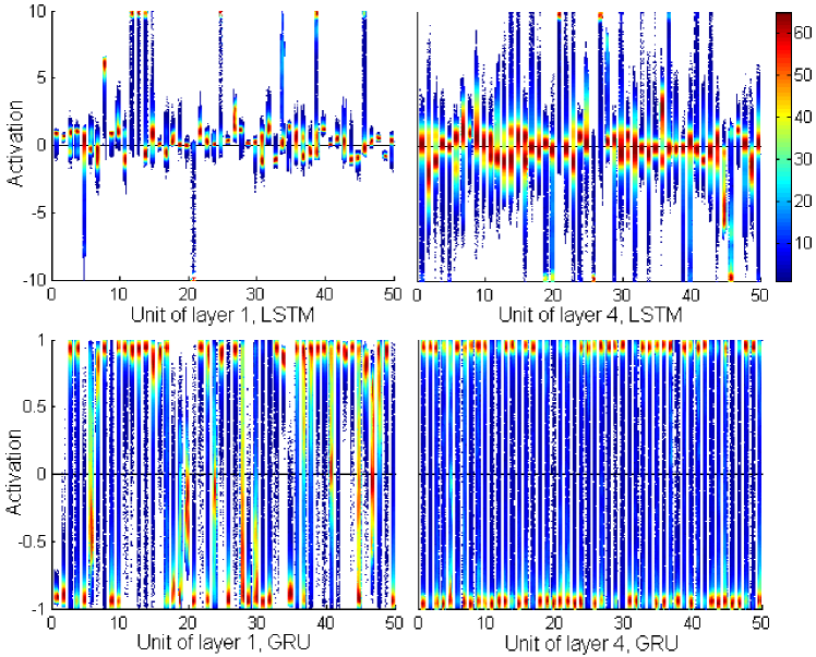
Fig. 1: The distribution of cell activations of LSTM RNN (above) and GRU RNN (below).

4.2 Temporal trace

The second experiment investigates the evolution of the cell activations when performing recognition. This is achieved by drawing the cell vectors of all the frames using the t-SNE tool [20] when decoding an utterance. The results are shown in Fig. 2, where the temporal traces for the four layers are drawn in the plots from top to bottom. An interesting observation is that the traces are much more smooth with LSTM than with GRU. This indicates that LSTM tends to remember more than GRU: with a long-term memory, the novelty of the current time is largely averaged out by the past memory, leading to a smooth temporal trace. For GRU, new experience is quickly adopted and so the memory tends to change drastically. When comparing the memory traces at different layers, it can be seen that for GRU, the traces become more smooth at higher-level layers, whereas this trend is not clear for LSTM. This suggests that GRU can trade off innovation and memorization at different layers: at low-level layers, it concentrates on innovation, while at high-level layers, memorization becomes more important. This is perhaps an advantage and is analog to our human brain where the low-level features change abruptly while the high-level information keeps evolving gradually.

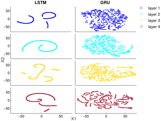
Fig. 2: The temporal trace of LSTM and GRU.

4.3 Memory robustness

The third experiment tests the robustness of LSTM and GRU with noise interruptions. Specially, during the recognition, a noise segment is inserted into the speech stream, and we observe the influence of this noise segment by visualizing the difference in cell values caused by the noise insertion. The results are shown in Fig. 3.

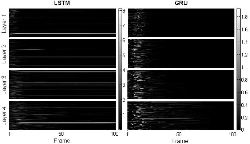
Fig. 3: The memory change with noise segment insertion.

It can be seen that both units accumulate longer memory at higher-level layers, and GRU is more robust than LSTM in noisy conditions. With LSTM, the impact of the noise lasts almost till the end on some cells, even at the final layer for which the units are supposed to be noise robust. With GRU, the impact lasts just a few frames. This demonstrates a big advantage of GRU, and double confirms the observation in the second experiment that GRU remembers less than LSTM.

5 Application to structure design

The visualization results shown in the previous section demonstrate that LSTM and GRU possess different properties in both information encoding and temporal evolution. By these differences, it is not easy to tell which model is better in a particular task. In speech recognition, the experimental results in Section 3.2 seemingly demonstrate that GRU is more suitable. This can be explained by the fact that speech signals are pseudo-stationary and typical durations of phones are not longer than $50$ frames. This means that shorter memory is likely an advantage, particularly when the noise robustness is considered. Inspired by these observations, we introduce some modifications to LSTM and/or GRU, both resulting in performance gains.

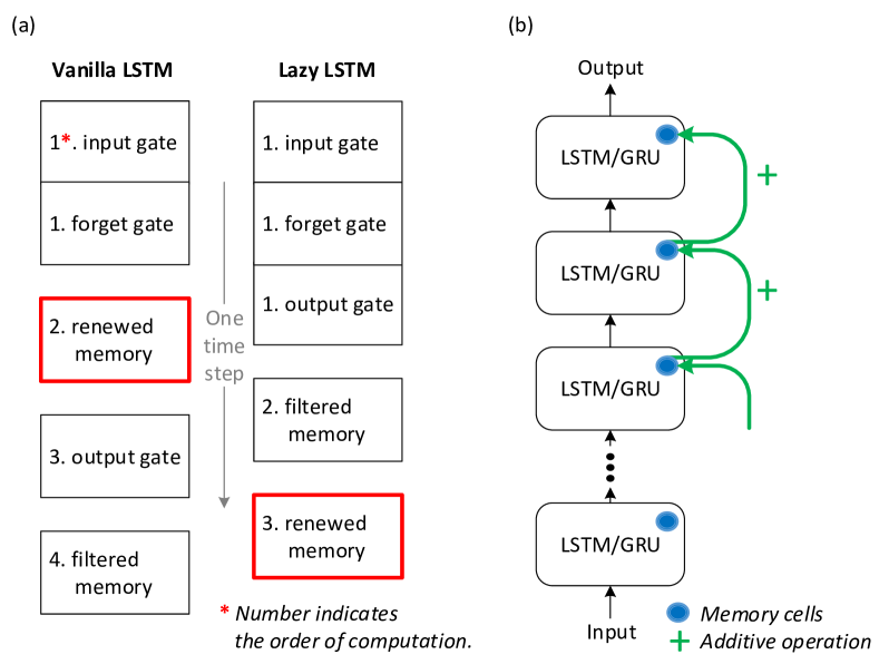
Fig. 4: Two modifications for gated RNNs. (a) Lazy cell update; (b) Shortcut connection for residual learning.

5.1 Lazy cell update

A difference between LSTM and GRU, as shown in Section 3.1, is that GRU updates cells as the final step, while LSTM updates cells before computing output gates. To study the impact of the lazy update with GRU, we reorder the computation in LSTM as shown in Fig. 4 (a). The recognition results are presented in Table 2, and the temporal trace with lazy update is shown in Fig. 5 (a). Note that only the final LSTM layer has been modified.

From the results, it can be seen that the lazy update does improve performance of LSTM. From the temporal trace, it seems that the modified LSTM behaves more like a GRU: the trace is less smooth, allowing quicker adoption of new input. This demonstrates the short-memory behavior of GRU is possibly an important factor for the good performance, and this behavior is closely related to the lazy cell update.

	WER%
Recurrent Layers	Baseline	Lazy Update
1	10.96	10.18
2	9.97	9.48
4	9.67	9.10

Table 2: Performance of LSTM without/with lazy cell update.

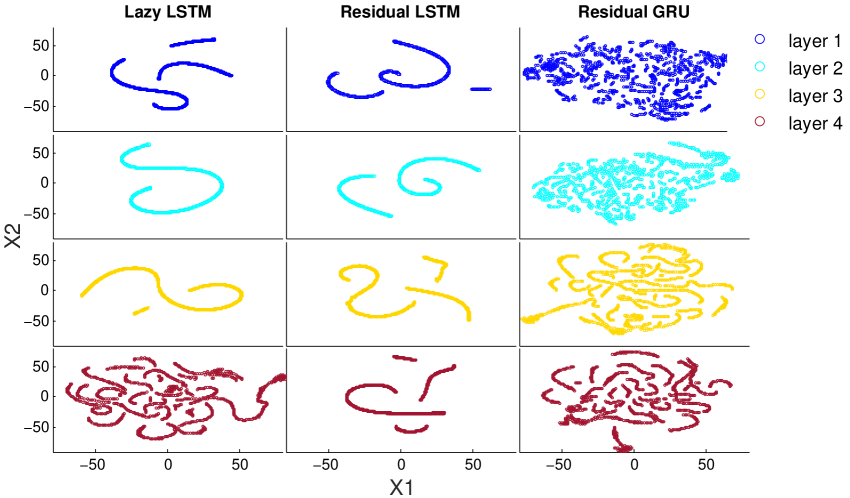
Fig. 5: Memory trace of (a) LSTM with lazy update (left); (b) LSTM with shortcut connections (center); (c) GRU with shortcut connections (right).

5.2 Shortcut connections for residual learning

Another modification is inspired by the visualization result that the gates at high-level layers show a similar pattern [12]. This implies that the cells in high-level layers are mostly learned by residual. This is also confirmed by recent research on residual net [21]. We borrow this idea and add explicit shortcut connections alongside the gated units, so that the main path is enforced to learn residual. This is shown in Fig. 4 (b).

		WER%
System	Recurrent Layers	Baseline	Residual Learning
LSTM	4	9.67	9.53
	6	9.47	9.33
GRU	4	9.32	9.23
	6	9.32	9.10

Table 3: Performance of LSTM/GRU with memory residual connections.

The results with the residual learning are shown in Table 3, and the temporal traces are shown in Fig 5 (b)(c). These results show that adding shortcut connections indeed introduces consistent performance gains with both LSTM and GRU. The temporal traces at different layers seem more consistent (note that for t-SNE, only the topological relations are important). This is particularly evident for GRU, where the third layer now can remember some short-time events as well. This is expected, as the information flow is quicker and easier with the shortcut connections.

6 Conclusion

This paper presented some visualization results for gated RNNs, and in particular focused on comparison between LSTM and GRU. The results show that the two gated RNNs use different ways to encode information and the information in GRU is more distributed. Moreover, LSTM possesses a long-term memory but it is also noise sensitive. Inspired by these observations, we introduced two modifications to enhance gated RNNs: lazy cell update and short connections for residual learning, and both provide interesting performance improvement. Future work will compare neural models in different categories, e.g., TDNN and RNN.

References

- [1] Li Deng and Dong Yu, “Deep learning: Methods and applications,” Foundations and Trends in Signal Processing, vol. 7, no. 3-4, pp. 197–387, 2013.
- [2] Alex Graves, A-R Mohamed, and Geoffrey Hinton, “Speech recognition with deep recurrent neural networks,” in Proceedings of IEEE International Conference on Acoustics, Speech and Signal Processing (ICASSP). IEEE, 2013, pp. 6645–6649.
- [3] Alex Graves and Navdeep Jaitly, “Towards end-to-end speech recognition with recurrent neural networks,” in Proceedings of the 31st International Conference on Machine Learning (ICML), 2014, pp. 1764–1772.
- [4] Hasim Sak, Andrew Senior, and Françoise Beaufays, “Long short-term memory recurrent neural network architectures for large scale acoustic modeling,” in Proceedings of the Annual Conference of International Speech Communication Association (INTERSPEECH), 2014.
- [5] Sepp Hochreiter and Jürgen Schmidhuber, “Long short-term memory,” Neural computation, vol. 9, no. 8, pp. 1735–1780, 1997.
- [6] Kyunghyun Cho, Bart Van Merriënboer, Dzmitry Bahdanau, and Yoshua Bengio, “On the properties of neural machine translation: Encoder-decoder approaches,” arXiv preprint arXiv:1409.1259, 2014.
- [7] Dario Amodei, Rishita Anubhai, Eric Battenberg, Carl Case, Jared Casper, Bryan Catanzaro, Jingdong Chen, Mike Chrzanowski, Adam Coates, Greg Diamos, et al., “Deep speech 2: End-to-end speech recognition in english and mandarin,” arXiv preprint arXiv:1512.02595, 2015.
- [8] Dumitru Erhan, Yoshua Bengio, Aaron Courville, and Pascal Vincent, “Visualizing higher-layer features of a deep network,” Tech. Rep., University of Montreal, 2009.
- [9] Matthew D Zeiler and Rob Fergus, “Visualizing and understanding convolutional networks,” in European Conference on Computer Vision. Springer, 2014, pp. 818–833.
- [10] Karen Simonyan, Andrea Vedaldi, and Andrew Zisserman, “Deep inside convolutional networks: Visualising image classification models and saliency maps,” arXiv preprint arXiv:1312.6034, 2013.
- [11] Michiel Hermans and Benjamin Schrauwen, “Training and analysing deep recurrent neural networks,” in Advances in Neural Information Processing Systems (NIPS), 2013, pp. 190–198.
- [12] Andrej Karpathy, Justin Johnson, and Li Fei-Fei, “Visualizing and understanding recurrent networks,” arXiv preprint arXiv:1506.02078, 2015.
- [13] Ákos Kádár, Grzegorz Chrupała, and Afra Alishahi, “Representation of linguistic form and function in recurrent neural networks,” arXiv preprint arXiv:1602.08952, 2016.
- [14] Jiwei Li, Xinlei Chen, Eduard Hovy, and Dan Jurafsky, “Visualizing and understanding neural models in nlp,” arXiv preprint arXiv:1506.01066, 2015.
- [15] Yajie Miao, Jinyu Li, Yongqiang Wang, Shi-Xiong Zhang, and Yifan Gong, “Simplifying long short-term memory acoustic models for fast training and decoding,” in 2016 IEEE International Conference on Acoustics, Speech and Signal Processing (ICASSP). IEEE, 2016, pp. 2284–2288.
- [16] Junyoung Chung, Caglar Gulcehre, KyungHyun Cho, and Yoshua Bengio, “Empirical evaluation of gated recurrent neural networks on sequence modeling,” arXiv preprint arXiv:1412.3555, 2014.
- [17] Daniel Povey, Arnab Ghoshal, Gilles Boulianne, Lukas Burget, Ondrej Glembek, Nagendra Goel, Mirko Hannemann, Petr Motlicek, Yanmin Qian, Petr Schwarz, et al., “The kaldi speech recognition toolkit,” in IEEE 2011 workshop on automatic speech recognition and understanding. IEEE Signal Processing Society, 2011, number EPFL-CONF-192584.
- [18] Daniel Povey, Xiaohui Zhang, and Sanjeev Khudanpur, “Parallel training of dnns with natural gradient and parameter averaging,” arXiv preprint arXiv:1410.7455, 2014.
- [19] Zhiyuan Tang, Ying Shi, Dong Wang, Yang Feng, and Shiyue Zhang, “Visualization analysis for recurrent networks,” Tech. Rep., CSLT, Tsinghua University, 2016, http://cslt.org/mediawiki/images/6/6a/Visual.pdf.
- [20] Laurens van der Maaten and Geoffrey Hinton, “Visualizing data using t-sne,” Journal of Machine Learning Research, vol. 9, no. Nov, pp. 2579–2605, 2008.
- [21] Kaiming He, Xiangyu Zhang, Shaoqing Ren, and Jian Sun, “Deep residual learning for image recognition,” arXiv preprint arXiv:1512.03385, 2015.