Gene networks accelerate evolution by fitness landscape learning

Abstract

We consider evolution of a large population, where fitness of each organism is defined by many phenotypical traits. These traits result from expression of many genes. We propose a new model of gene regulation, where gene expression is controlled by a gene network with a threshold mechanism and there is a feedback between that threshold and gene expression. We show that this regulation is very powerful: depending on parameters we can obtain any functional connection between thresholds and genes. Under general assumptions on fitness we prove that such model organisms are capable, to some extent, to recognize the fitness landscape. That fitness landscape learning sharply reduces the number of mutations necessary for adaptation and thus accelerates of evolution. Moreover, this learning increases phenotype robustness with respect to mutations. However, this acceleration leads to an additional risk since learning procedure can produce errors. Finally evolution acceleration reminds races on a rugged highway: when you speed up, you have more chances to crash. These results explain recent experimental data on anticipation of environment changes by some organisms.

1 Introduction

The central biological paradigm is that evolution goes via gene mutations and selection. This process may be represented as a walk in a fitness landscape leading to a fitness increase and a slow adaptation (Orr 2005). According to classical ideas this walk can be considered a sequence of small random steps with small phenotypic effects. However, in the 1980s, new experimental approaches were developed, in particular, quantitative trait locus (QTL) analysis. In QTL analysis, the genetic basis of phenotypic differences between populations or species can be analyzed by mapped molecular markers. Genetic and molecular tools allow us to find some genetic changes that underlie adaptation. Results (see, for example, Zeyl (2005)) show that evolution can involve genetic changes of relatively large effect and, in some cases, the total number of changes are surprisingly small. Another intriguing fact is that organisms are capable to make an adaptive prediction of environmental changes (Mitchell et al. 2009).

To explain these surprising facts new evolutionary concepts were suggested (see the review by Watson and Szathmáry (2015) and references therein). The main idea is that population can “learn” (recognize) fitness landscapes (Chastain et al. 2014; Parter et al. 2008; Watson and Szathmáry 2015). This learning can explain the adaptive prediction effect.

A mathematical basis for investigation of evolution learning problems is developed by Valiant (2006, 2009). However, this work uses a simplified model, where organisms are represented as Boolean circuits seeking for an “ideal answer” on environmental challenges. These circuits involve $n$ Boolean variables that can be interpreted as genes, and the ideal answer maximizes the fitness. A similar model was studied numerically by Parter et al. (2008) to confirm the theory of “facilitated variation” explaining appearance of genetic variations, which can lead to large phenotypic ones. In the work by Livnat et al. (2014) an evolution theory of the Boolean circuits is advanced. It is shown that, under some conditions—weak selection, see Nagylaki (1993))—a polynomially large population over polynomially many generations (polynomial in $n$) will end up almost surely consisting exclusively of satisfying truth assignments. This theorem can shed light on the problem of the evolution of complex adaptations since that satisfiability problem can be considered as a rough mathematical model of adaptation to many constraints.

In (Chastain et al. 2014) it is shown that, in the regime of weak selection, population evolution can be described by the multiplicative weight update algorithm (MWUA), which is a powerful tool, well known in theoretical computer science and generalizing such famous algorithms as Adaboost and others (Arora et al. 2012). Note that in (Chastain et al. 2014) infinitely large populations are investigated whereas the results of (Livnat et al. 2014) hold only for finite populations and take into account genetic drift.

In this paper, we consider a new model, which extends the previous ones and describes the Boolean circuits with genetic regulation. By this model, we investigate a connection of the landscape learning problems with evolution acceleration and canalization. The canalization effect, pioneered in the paper by Waddington (1942) means that the phenotype robustness becomes greater. Canalization is a measure of the ability of a population to produce the same phenotype regardless of variability of its environment or genotype (Waddington 1942). In our case it means robustness of adapted phenotypes with respect to mutations.

Two seminal papers describe connections between evolution and canalization (phenotypic buffering) quite differently. Waddington (1942) claims that phenotypic buffering is needed for adaptation. According to Waddington, there is a connection between canalization and genetic assimilation of an acquired character that was demonstrated experimentally by Waddington (1953) for a population of Drosophila under a heat shock. However, based on other impressive experiments with Drosophila, Rutherford and Lindquist (1998) say the exact opposite, namely, that the phenotypic buffering shutdown is required for adaptive changes. In the concept stated by Rutherford and Lindquist (1998) and other works, for example by Masel and Siegal (2009), some genes can serve as capacitors. When the population is under a stress (a heat shock, radiation, or chemical reagents), buffering falls and capacitors release a hidden genetic information that leads to new species formation. A mathematical model for this effect is proposed in (Grigoriev et al. 2014).

In this paper, we aim to show that, in a fixed environment, genes can serve as learners. We show, by analytical methods, that the gene circuits having such regulation networks are capable to recognize, to some extent, fitness landscapes. Indeed, if an organism has survived within a long period, this fact brings an important information, which can be used for gene regulation system training. Biological interpretation of this fact is simple: if a population is large enough and mutations are sufficiently seldom, selection eliminates all negative mutants. So, if an organism is viable and it was affected by a mutation (which is not neutral, i.e. changed phenotype and the fithess), then with probability close to $1$ that mutation is positive. We obtain mathematical results, which allows us to estimate evolution acceleration and canalization due to that learning procedure. Note that the biological interpretation of evolution acceleration is also quite transparent: learning by gene regulation networks sharply reduces the number of mutations, which are necessary to form a phenotypic trait useful for adaptation.

Note that we use a model more sophisticated than the ones studied by Livnat et al. (2014); Valiant (2009). In contrast to these works, our model is not simply a Boolean circuit. Namely, Boolean circuits control formation of quantitative phenotypic traits, expressions of those phenotypic traits range in the whole interval $(0,1)$. However, in contrast to (Livnat et al. 2014; Valiant 2009), our circuits can be regulated, i.e., have a plasticity property. Note that biological ideas beyond that regulation mechanism were proposed, in a simpler and informal manner, still in (Stern 1958). Stern introduced thresholds which determine how many genes should be activated to express a trait useful for survival and explained mechanisms of gene assimilation suggested by Waddington (1942). Actually, one can consider the model of this paper as a combination of models (Livnat et al. 2014; Valiant 2009; Stern 1958). We show that fitness landscape learning is possible only if there exists a a non trivial connection between a gene control of phenotype (morphogenesis) and the gene regulation developed as a result of evolution.

2 Materials and Methods

In this section, we describe our model and our mathematical approach.

2.1 Genom

We assume that the genotype can be described by Boolean strings

$$s=(s_{1},s_{2},\ldots,s_{N}),\quad s_{i}\in S=\{0,1\},\quad s\in S^{N},$$ (1)

i.e., a gene can either be in an active state (switched on), or in a passive one (switched off).

2.2 Phenotypic traits

Phenotypic traits are controlled by many genes (Orr 2005). We consider levels $f_{j}$ of expressions of those phenotypic traits as real variables range in $(0,1)$. Then the vector $f=(f_{1},\ldots,f_{m})$ can be considered formally as an organism phenotype. We suppose that

$$f_{j}=f_{j}(s,h_{j}),\quad j=1,\ldots,m,$$ (2)

where $f_{j}\in[0,1]$ is a real valued function of the Boolean string $s$ (which is the genotype) and a real valued variable $h_{j}$, which is a tuning parameter for gene regulation (we will describe it in more detail below).

Only a part of $s_{i}$ involved in $f_{j}$. Namely, for each $j$ we have a set of indices $K_{j}=\{i_{1},i_{2},\ldots,i_{n_{j}}\}$ such that $f$ depends on $s_{i}$ only for $i\in K_{j}$, i.e.,

$$f_{j}(s,h)=f_{j}(s_{i_{1}},s_{i_{2}},\ldots,s_{i_{n_{j}}},h_{j})$$

where $i_{l}\in K_{j}$ and $n_{j}$ is the number of elements in $K_{j}$ ($n_{j}$ is the number of genes involved in the control of the trait expression).

Another possible interpretation of $f_{i}$ is as follows. Multicellular organisms consist of cells of different types. One can suppose that the organism phenotype is defined completely by the corresponding cell pattern. The cell type $j$ is determined by morphogenes, which can be identified as gene products or chemical reagents that can change cell type (or genes that code for that chemical reagents that can determine cell types or cell-cell interactions and then finally the cell pattern). The morphogene activity is defined by (2).

We suppose that the following assumption is satisfied:

Assumption M. Assume that activities $f_{j}(s,h)$ have the following properties.

M1 All $f_{j}(s,h_{j})$ are functions of real valued parameter $h_{j}$. For each fixed $s$

$$f_{j}(s,h_{j})\to 0\ (h_{j}\to-\infty),$$ (3)

and

$$f_{j}(s,h_{j})\to 1\ (h_{j}\to+\infty)$$ (4)

M2 The sets $K_{j}$ are independent random subsets of the set of all genes consisting at most $K$ elements:

$$K_{j}=\{i_{1},\ldots,i_{n_{j}}\},\quad i_{l}\in\{1,\ldots,N\},\quad 0<n_{j}\leq K,$$ (5)

and

$$Km/N=\alpha<1.$$ (6)

The second assumption entails that only a part of all genes is involved in control of the phenotypic expression. We denote the number of genes involved in regulation of $f_{j}$ by $N_{r}$. Note that (6) shows that $N_{r}=\sum n_{j}\leq Km$.

Condition M1 implies that there exists a parameter in $f_{j}$, which can control this function. Assumption M2 means that the genes are organized, in a sense, randomly (note that this assumption plays a key role in probabilistic methods for problems with many constraints such as $k$-SAT (Friedgut 1999)). The condition $\alpha\ll 1$ means that we have a "gene freedom", i.e., we have sufficiently many genes with respect to the number of the traits. This freedom yields that the probability of gene pleiotropy in the gene regulation is sufficiently small for large genomes.

Let us consider a biological interpretation of $h_{j}$. We consider $h_{j}$ as a tuning parameter that defines level and sign of gene regulation for $j$-th phenotypocal trait. The genes produce a number of different gene products (proteins, miRNA, tRNA). Some of these products can serve as transciption factors involved in gene expression regulation. The parameters $h_{j}$ determine intensities and signs of this regulation. Condition (3) and (4) mean that for large negative $h$ one has a strong repression of $f_{j}$ expression while for large positive $h$ the expression level is close to almost maximal one.

Consider a biologically natural example, where the assumptions M1 and M2 hold. This example is inspired by the work (Stern 1958) and model (Mjolsness et al. 1991). Let

$$f_{j}=z_{j}=\sigma(\sum_{i=1}^{N}w_{ji}{s_{i}}-h_{j}),$$ (7)

where $j=1,\ldots,m$. Here $\sigma(S)$ is a sigmoidal function of $S$ such that

$$\sigma(+\infty)=1,\quad\sigma(-\infty)=0,\quad\sigma^{{}^{\prime}}(S)>0.$$ (8)

As an example, we can take $\sigma(S)=(1+\exp(-bS))^{-1}$, where $b>0$ is a sharpness parameter. Note that for large $b$ this sigmoidal function tends to the step function and for $b=+\infty$ our model becomes a Boolean one. Some experimental results show that miRNA control involves a threshold mechanism (Mukherji et al. 2011). Note that threshold mechanisms are omnipresent in gene networks (Kauffman and Weinberger 1989; Mjolsness et al. 1991) and fundamental for neural networks (Hopfield 1982). The parameters $h_{j}$ are important tools of gene regulation since they affect the gene circuit structure and define circuit plasticity. The idea to use such a parameter was proposed by Stern (1958), see also (Livnat et al. 2014) for interesting comments on the connection with evolution.

Let us introduce the matrix $W$ of size $m\times N$ with entries $w_{ij}$.

The coefficients $w_{ji}$ determine the effects of terminal differentiation genes (Grigoriev et al. 2014), and hence encodes the genotype-phenotype map. We assume that $w_{ji}\in\{[-1-\gamma,-1],0,[1,1+\gamma]\}$, where $\gamma$ is a positive parameter. Moreover, we assume that the coefficients $w_{ji}$ are random, with the probability that $w_{ji}>0$ or that $w_{ji}<0$ is $\beta/2N$, where $\beta>0$ is a parameter. This quantity $\beta$ defines a genetic redundancy, i.e., averaged numbers of genes involved in regulation of a trait. Note that then assumption M2 holds and $K\approx\beta$ for large $\beta$.

The number $\gamma$ is a measure of phenotypic buffering. The condition $\gamma=0$ means that there is no phenotypic buffering, $\gamma>0$ means that the buffering works; larger $\gamma$ leads to a buffering increase.

Let us introduce the matrix $W$ of size $m\times N$ with the entries $w_{ji}$ and the corresponding the sign matrix $S(W)$ with entries $s_{ij}=sign(w_{ij})$, where $sign(x)=1$ for $x>0$, $sign(x)=-1$ for $x<0$ and $sign(0)=0$. The matrix $S(W)$ plays an important role below; that matrix determines qualitatively the control of the phenotypical traits by the genes. If $s_{ji}>0$ this means that activation of $i$ -th gene leads to an increase of $j$-th trait expression; if $s_{ji}<0$ then activation of $i$ -th gene leads to a decrease of $j$-th trait expression; at last, if $s_{ji}=0$ this means that the $i$-th gene is not involved in the control of $f_{j}$.

2.3 Fitness

Actually we know a little about fitness of multicellular organisms, see e.g. the review by (Franke et al. 2011). Recall some known fitness models.

The random field models assign fitness values to genotypes independently from a fixed probability distribution. They are close to mutation selection models introduced by Kingman (1978), and can be named House of Cards (HoC) model. The best known model of this kind is the NK model introduced by Kauffman and Weinberger (1989), where each locus interacts with $K$ other loci. Rough Mount Fuji (RMF) models are obtained by combining a random HoC landscape with an additive landscape models (Aita et al. 2001).

In this work, we use the classical approach of R. Fisher, namely, phenotype-fitness maps. Our phenotype is given by $f$, i.e., we assume that the phenotype is completely determined by the phenotype trait expression, and thus the fitness depends on $s$ via $f_{j}$.

We can express the relative fitness via an auxiliary function $W(s)$ by relation

$$F=C_{M}\exp(W(s)),$$ (9)

where a constant $C_{M}$ is proportional to the number of progenies. Below we refer $W$ as a fitness potential, and we assume that

$$W=\sum_{j=1}^{L}b_{j}f_{j}(s,h_{j}).$$ (10)

We consider fitness as a numerical measure of interactions between the phenotype and an environment. For a fixed environment, this idea gives us the fitness of classical population genetics. A part of the fitness, however, depends on the organism developing properly and for now we represent it as independent of the environment (we are aware that this is not always true).

A part of coefficients $b_{j}$ may be negative and the other part is positive. The corresponding contributions will be denoted by $W^{I}$ and $W^{E}$, respectively:

$$W^{I}=\sum_{j=1,b_{j}<0}^{L}b_{j}f_{j}(s,h_{j}),$$ (11)

$$W^{E}=\sum_{j=1,b_{j}>0}^{L}b_{j}f_{j}(s,h_{j}).$$ (12)

The first function $W^{I}(s)$ is associated with the internal fitness and the second $W^{E}(s)$ determines an interaction between the organism and its environment. If we assume that $f_{j}$ are morphogene concentration levels, which control cell types, then the part $W^{I}$ measures a viable development in terms of formation of correct cell types. Each cell type is determined by the corresponding morphogene activity $f_{j}$. Another component of fitness, $W^{E}(s)$ depends on the environment and it describes how well the organism is adapted to it. The terms $f_{i}$ involved in $W^{E}$ can be interpreted as gene responses on the environment. The terms with $b_{i}<0$ involved in $W^{I}$ can for example define a fitness reduction caused by formation of non-necessary (excess) cells. We assume that in a “normal” state, that corresponds to the maximal fitness, all $f_{j}$ in $W^{I}$ are close to zero. When such a $f_{j}\approx 1$, this can be interpreted as appearance of a "bad" cell, for example, a cancer one.

Another possible interpretation of $W^{I}$ is that a larger expression of some phenotypical traits can decrease chances of the organism to be viable in a given environment.

Note that this model (10) can describe gene epistatic effects via dependence of $f_{j}$ on $s$ if $f_{j}$ are nonlinear in $s$.

2.4 Population dynamics model

For simplicity, mainly we consider populations with asexual reproduction (although a part of results is valid for sexual reproduction, see comments in the end of this subsection).

In each generation , there are $N_{\mathrm{pop}}(t)$ individuals, the genome of each of them is denoted by $s(t)$, where $t=0,1,2,\ldots$ stands for the evolution step number). Following the classical ideas of Wright -Fisher model, we suppose that generations do not overlap. In each generation (i.e., for each $t$), the following three steps are performed:

1. Each individual $s$ at each evolution step can mutate with probability $p_{\mathrm{mut}}$.

2. At evolution step $t$ each individual produces $k$ progenies randomly with the probability $P_{k}$ defined by the Poisson law

   $$P_{k}=\frac{q(t)^{k}}{k!}\exp(-q(t))=\Lambda(k,q(t)),$$ (13)

   where $q=F/\bar{F}(t)$, $F$ is the fitness of that individual and $\bar{F}(t)$ is the averaged fitness of the population at the moment $t$ defined by.

   $$\bar{F}(t)=\sum_{s\in S(t)}X(s,t)F(s(t)),$$ (14)

   where $\bar{F}(t)$ can be interpreted as the averaged population fitness at the moment $t$ , $S(t)$ the set of the genotypes represented in the population at the moment $t$ (the genetic pool) and $X(s,t)=N(s,t)/N_{pop}(t)$ is the frequency of genotype $s$. Here $N(s,t)$ denotes the number of the population members with genotype $s$ at the step $t$.

3. If $N_{\mathrm{pop}}(t)>N_{\mathrm{popmax}}$, where $N_{\mathrm{popmax}}$ is some number, individuals are removed randomly until $N=N_{\mathrm{popmax}}$.

After each selection step, there occur mutations in the genotypes, which create a new genetic pool and then a new round of selection starts. The last condition express the fundamental ecological restriction that all environments have restricted resources only (bounded capacity), therefore, they can supply only populations bounded in size. However, if the evolution time $T$ is bounded, $t=0,1,\ldots T$ and $N_{pop}(t)\gg 1$ then we can remove the last condition since by (13) and the Central Limit Theorem one can show that fluctuations of the population size are small: $|N_{\mathrm{pop}}(t+1)-N_{pop}(t)|\ll N_{\mathrm{pop}}(t)$. Thus then the population is ecologically stable and the population size fluctuate weakly. The condition (3) is really essential for small populations only (which considered by numerical simulations).

In the limit case of infinitely large populations we use the following dynamical equations for the frequency $X(s,t)$ of the genotype $s$ in the population at the moment $t$:

$$X(s,t+1)=\bar{F}(t)^{-1}X(s,t)F(s(t)),\quad X(s,0)=X_{0}(s).$$ (15)

Equations (15) do not take into account the genetic drift. For large but finite populations $N_{\mathrm{popmax}}$ we should take into account this effect. Moreover, it is important that our populations and organisms can extinct.

Equations (15) and (14) describe a change of the genotype frequencies due to selection at the $t$-th evolution step. The same equations govern evolution in the case of sexual reproduction in the limit of weak selection (Nagylaki 1993; Chastain et al. 2014). Note that for an evolution defined by (14), (15) the averaged fitness $\bar{F}(t)$ satisfies Fisher’s theorem, namely, this function does not decrease in evolution step $t$ and we have $\bar{F}(t+1)\geq\bar{F}(t)$.

Note that for simplicity we consider the point mutations (see the point (i) above) although it is well known that mutation process is much more complicated. However, some of our analytical results are valid for more general situations.

2.5 Gene regulation

We introduce the regulatory genes $y_{j}$, where $j=1,\dots,n$ and $n$ is the number of regulatory genes. They may be hubs in the networks, i.e., interact with many genes. The activities of $y_{j}$ are real numbers defined by

$$y_{j}(s)=\sigma_{R}(a_{j1}s_{1}+\ldots+a_{jN}s_{N}-\tilde{h}_{j}),$$ (16)

where $\sigma_{R}$ is a sigmoidal function (one can take here a linear approximation, for example, $\sigma_{R}(x)=a_{R}x$, where $a_{R}$ is a coefficient ), $a_{ji}$ are real valued coefficients and $\tilde{h}_{j}$ are thresholds.

The feedback between genotype $s$ and the parameters $h_{j}$ is defined by a dependence of thresholds $h_{j}$ via the quantities $y_{j}$’s:

$$h_{j}(s)=\bar{h}_{j}-r_{F}\sum_{\tau=0}^{\tau_{r}}\sum_{k=1}^{n}g_{jk}(\tau)y_{k}(s(t-\tau)),$$ (17)

where $g_{ik}$ are positive random numbers, $r_{F}>0$ is a feedback parameter and $\bar{h}_{j}$ are positive constants. The parameter $\tau_{r}$ defines the memory of the regulation network.

If we introduce the shift map $T_{\tau}$ defined on sequences $s(t)$ by $T_{\tau}s(t)=s(t-\tau)$, then $h_{j}$ becomes a function of shifted Boolean arguments

$$h_{j}=h_{j}(s(t),s(t)^{(1)}),\ldots,s(t)^{(\tau_{r})}).$$ (18)

where $s^{(\tau)})=T_{\tau}s(t)=s(t-\tau)$.

2.6 Main assumptions

A. We assume that the mutation probability $p_{\mathrm{mut}}$ is small and the time $T$ of evolution is large:

$$\theta=Np_{\mathrm{mut}}\ll 1,\quad T\gg\log(N_{\mathrm{popmax}}).$$ (19)

B. We choose initial genotypes randomly from a gene pool and assign them to organism. This choice is invariant with respect to the population member, i.e,. the probability to assign a given genotype $s$ for a member does not depend on that member.

2.7 Complexity of the model

2.7.1 Connections with hard combinatorial problems

Adaptation (i.e., maximization of the fitness) is a very hard problem, since in evolution history we observe coevolution of many traits. As an example of such coevolution, we can consider mammal evolution. Long evolution of mammals is marked by development of many traits. Mammals are noted for their large brain size relative to body, size, compared to other animal groups, moreover, mammals developed many other features: lactation, hair and fur, erect limbs, warm bloodness etc. It is not clear how a random gradual search based on small random mutation steps and selection only, can resolve such complex adaptation problem with many constraints and to create a complex phenotype with many features.

To show that the model stated above reflects this biological reality, let us consider the case, where $f_{j}$ are defined by relations (7) and assume that

i) $\sigma$ is the step function;

ii) $b_{j}>0$.

As a consequence of the second assumption $F$ attains its maximum for $f_{1}=1,f_{2}=1,\ldots,f_{m}=1$. Let us show that, even in this particular case, the problem of the fitness maximization with respect to $s$ is very complex. In fact, for a choice of $h_{j}$ it reduces to the famous NP-complete problem, so-called $k$-SAT, which has been received a great attention of mathematicians, computer scientists, and biologists the last decades (see (Cook 1971; Levin 1973; Friedgut 1999; Moore and Mertens 2011)). The $k$-SAT can be formulated as follows.

$k$-SAT problem Let us consider the set $V_{n}=\{s_{1},\ldots,s_{n}\}$ of Boolean variables $s_{i}\in\{0,1\}$ and a set ${\mathcal{C}}_{m}$ of $m$ clauses. The clauses $C_{j}$ are disjunctions (logical ORs) involving $k$ literals $z_{i_{1}},z_{i_{2}},\ldots,z_{i_{k}}$, where each $z_{i}$ is either $s_{i}$ or the negation $\bar{s}_{i}$ of $s_{i}$. The problem is to test whether one can satisfy all of the clauses by an assignment of Boolean variables.

Cook and Levin 1971; 1973 have shown that $k$-SAT problem is NP-complete and therefore in general it is not feasible in a reasonable running time. In subsequent studies—for instance, by Friedgut (1999)—it was shown that $k$-SAT of a random structure is feasible under the condition that $m<2^{k}N$.

To see a connection with $k$-SAT, consider relation (7) under assumption $w_{ij}=1$ and set $h_{j}=-C_{j}+0.5$, where $C_{j}$ is the number of negative $w_{ji}$ in the sum $S_{j}=\sum_{i=1}^{N}w_{ji}{s_{i}}$. Under such choice of $h_{j}$ terms $\sigma(S_{j})$ can be represented as disjunctions of literals $z_{j}$. Each literal $z_{j}$ equal either $s_{j}$ or $\bar{s}_{j}$, where $\bar{s}_{j}$ denotes negation of $s_{j}$. To maximize the fitness we must assign such $s_{j}$ that all disjunctions will be satisfied. If we fix the number $k$ of the literals participating in each disjunction (clause), this assignment problem is $k$-SAT formulated above.

2.7.2 Biological interpretation of $k$-SAT

Reduction to the $k$-SAT is a transparent way of representing the idea that multiple constraints need to be satisfied. The quantity $k=\beta$ define the gene redundancy and the probability of gene pleiotropy. For larger $\beta$ this probability is smaller. The threshold parameter $h_{j}$ and $\beta$ define the number of genes, which should be flipped to attain a need expression level of the trait $f_{j}$. Mathematical results mentioned above say us that for a fixed $N$ and $m$ constraints can be satisfied for sufficiently large $\beta>\beta_{0}(N,m)$ only.

Note that there are important differences between $k$-SAT in Theoretical Computer Science and the fitness maximization problem. First, the signs of $b_{j}$ are unknown for real biological situations since the fitness landscape is unknown. The second, our adaptation problem involves the threshold parameters $h_{j}$ (see (7)). In contrast to Computer Science Theory, in our case the Boolean circuit has a plasticity, i.e., $h_{j}$ are not fixed.

If $b_{j}$ are unknown, the adaptation (the fitness maximization) problem becomes even harder because we do not know the function to optimize. Therefore, many algorithms for $k$-SAT are useless for biological adaptation problems. Below nonetheless we will obtain some analytical results under assumption that $b_{j}$ are random.

2.7.3 How to accelerate evolution? Main ideas

To overcome the computational hardness of our model, we apply the following ideas. By assumption M2 we use the randomness of the gene organization of expression and a small probability of gene pleiotropy. Moreover, for an organism survival it is not obligatory to attain the global maximum of the fitness, it is enough to attain a fitness value which is greater than fitnesses of other competing organisms.

However, the key idea inspired by the paper of Stern (1958) is as follows. Suppose a fitness landscape learning is possible and the signs of $b_{j}$ become known as a result of evolution (we will describe in the next sections how that learning can work). Let, for example, $b_{10}>0$. Then one can use circuit plasticity, i.e., a possibility to change $h_{10}$. In $k$-SAT, where $h_{j}$ are fixed, we seek for correct values $s_{i}$ involved in the right hand sides of (7) and it may be a computationally hard problem. In our case we just strongly increase or decrease of $h_{j}$, depending on the sign of $b_{j}$. It can be done by a gene regulation loop, described in subsection 2.5 but only under a correct choice the gene regulation scheme and parameters.

3 Results

The main results can be outlined as follows. Here we first use ideas analogous to ones given by Chastain et al. (2014) and also we propose an alternative method based on R. Fisher’s theorem. The second approach allows us to see for which fitness functions the fitness landscape learning is possible, to find optimal regulatory mechanisms and to investigate how this regulation depends on the fitness function structure. The gene regulation rate should be smaller for more rugged fitness functions.

3.1 Gene Regulation Power

The gene regulation defined by relations (16) and (17) is very powerful. It follows from the next assertion.

Theorem I

Let $H_{1}(s,s^{(1)},\ldots,s^{(\tau_{r})})$, …, $H_{m}(s,s^{(1)},\ldots,s^{(\tau_{r})})$ be functions of $\tau_{r}+1$ independent Boolean arguments $s,s^{(1)},\ldots,s^{(\tau_{r})}$. Then for any $\epsilon>0$ there exist parameters $a_{kl},\tilde{h}_{k},g_{ik}(0),\ldots,g_{ik}(\tau_{r})$ in (16) and (17) such that $h$ defined by (18) satisfies

$$|h_{j}(s,s^{(1)},\ldots,s^{(\tau_{r})})-H_{j}(s,s^{(1)},\ldots,s^{(\tau_{r})}|<\epsilon$$

for all $j$ and $s$.

Roughly speaking this means that gene regulation networks defined by (16) and (17) can approximate with arbitrary accuracy any prescribed time delayed feedback.

Proof. The theorem follows from approximation results for multilayered perceptrons. In fact, combination of (16) and (17) defines a straight forward neural network, namely, a perceptron with a single hidden layer. It is well known that such two layered perceptrons can approximate any Boolean target functions; for a proof see (Barron 1993).

3.2 Fitness Landscape Recognition Theorems

The following results are based on ideas close to ones given by Arora et al. (2012) and Chastain et al. (2014), but, for simplicity, we consider asexual reproduction. To obtain similar results for sexual reproduction, one can consider a weak selection regime and use classical results of Nagylaki (1993).

Let us introduce two sets of indices $I_{+}$ and $I_{-}$ (that we refer in sequel as positive sets and negative ones, respectively) such that $I_{+}\cup I_{-}=\{1,\ldots,m\}$. We have

$$I_{+}=\{j\in\{1,\ldots,m\}|b_{j}>0\},$$ (20)

$$I_{-}=\{j\in\{1,\ldots,m\}|b_{j}<0\}.$$ (21)

The biological interpretation of that definition is transparent: expression of the traits $f_{j}$ from the positive set $I_{+}$ increases the fitness. For the negative set $I_{-}$ that expression decreases the fitness.

Moreover, let us introduce useful auxiliary sets. Let $s$ and $s^{\prime}$ be two genotypes. Then we denote by $Diff(s,s^{{}^{\prime}})$ the set of positions $i$ such that $s_{i}\neq s_{i}^{{}^{\prime}}$:

$$Diff(s,s^{\prime})=\{i\in\{1,\ldots,N\}|\ s_{i}\neq s_{i}^{`}\}.$$

That set contains gene positions of the Boolean genome, where genes are flipped.

We also use notation

$$S_{b}=\sum_{j=1}^{m}b_{j,+},\quad b_{j,+}=\max\{b_{j},0\}.$$

Note that

$$\max_{s\in\Pi^{N}}F(s)\leq S_{b}.$$ (22)

Indeed, the fitness $F(s)$ attains the global maximum when $f_{j}=0$ for all $b_{j}<0$ and $f_{j}=1$ for all $b_{j}>0$.

Below we prove two theorems on fitness landscape learning. First we consider the case of infinitely large populations.

Evolution Recognition Theorem II.

Suppose that evolution of genotype frequencies $X(s,t)$ is determined by equations (14) and (15). Moreover, assume that

I for all $t\in[T_{1},T+T_{c}]$, where $T_{1},T_{c}>0$ the population contains two genotypes $s$ and $s^{\prime}$ such that the frequencies $X(s,t)$ and $X(s^{\prime},t)$ satisfy

$$X(s,T_{1}) = p_{0}>0,$$ (23)

$$X(s^{\prime},t) > p_{1}>0\quad\forall t\in[T_{1},T_{1}+T_{c}];$$ (24)

II we have

$$Diff(s,s^{`})\subset K_{j},$$ (25)

for some $j$, i.e., the genes $s_{i}$ such that $s_{i}\neq s_{i}^{`}$ are involved in a single regulation set $K_{j}$; moreover,

$$\delta=|f_{j}(s,h_{j})-f_{j}(s^{\prime},h_{j})|>0;$$

III

$$\kappa=min_{j}|b_{j}|>0,$$ (26)

and all $h_{j}$ are fixed on the interval $[T_{1},T_{1}+T_{c}]$.

Let $T_{c}$ satisfy

$$T_{c}>\frac{-\log(p_{0}p_{1})}{1+\varepsilon},\quad\varepsilon=\frac{\kappa\delta}{S_{b}},$$ (27)

Then, if

$$f_{j}(s,h_{j})<f_{j}(s^{\prime},h_{j}),$$ (28)

we have $j\in I_{+}$. If $f_{j}(s,h_{j})>f_{j}(s^{\prime},h_{j})$, then $j\in I_{-}$.

Before proving let us make some comments. The biological meaning of the theorem is very simple:

For fitness models, where unknown parameters $b_{j}$ are involved in a linear way, absence of pleiotropy in gene control of phenotypic traits $f_{j}$ lead to the fitness landscape learning in the limit of infinitely large populations.

Moreoever, let observe that we do not make no specific assumptions to the mutation nature, they may be point ones or more complicated but it is important that all gene variations between $s$ and $s^{\prime}$ are contained in a single regulatory set $K_{j}$.

Proof. The main idea beyond the proof is very simple. Since genetic drift is absent, the negative mutations leads to an elimination of mutant genotype from the population, the corresponding frequency becomes, for large times, exponentially small.

Consider the case (28). Let $j\in I_{-}$. Consider the quantity $Q(t)=\frac{X(s,t)}{X(s^{\prime},t)}$. We observe that

$$\Delta F=F(s)-F(s^{\prime})=b_{j}(f_{j}(s,h_{j})-f(s^{\prime},h_{j})).$$ (29)

Note that if $j\in I_{-}$ then assumptions II and III entail that

$$\Delta F\geq\kappa\delta.$$ (30)

Relation (30) implies

$$\frac{F(s)}{F(s^{\prime})}=1+\frac{\Delta F}{F(s^{\prime})}\geq 1+\frac{\Delta F}{\max F(s^{\prime})}.$$

Due to (22) one has

$$\frac{F(s)}{F(s^{\prime})}\geq 1+\varepsilon.$$

According to (15) the last inequality implies that for $T>T_{1}$

$$Q(T)\geq Q(T_{1})(1+\varepsilon)^{T-T_{1}}.$$ (31)

Let us note that $Q(T_{1})\geq p_{0}$ and $Q(T)\leq 1/p_{1}$.Therefore, one has

$$\frac{1}{p_{1}p_{0}}\geq(1+\varepsilon)^{T-T_{1}}.$$ (32)

This inequality leads to a contradiction for $T=T_{1}+T_{c}$ and $T_{c}$ satisfying (27) that finishes the proof.

Let us make some comments. The assertion is not valid if the set $Diff(s,s^{`})$ belongs to two different regulation sets $K_{i},K_{j}$. This effect is connected with a pleiotropy in the gene regulation. However, if assumption M2 holds then the pleiotropy probability is small for large genome lengths $N$.

Moreover, Theorem II can be extended on the case of finite but large populations when the genetic drift effect is small and under the assumption that the mutation probability also is small. We obtain the following assertion:

Evolution Recognition Theorem III

Consider the population dynamics defined by model 1-3 in subsection 2.4. Assume conditions A, B and M2 hold, and assumptions (23), (25), (26), (28) of the previous theorem are satisfied. Suppose $T_{c}$ satisfies the inequality

$$T_{c}>\frac{-\log(p_{0}p_{1})}{1+\varepsilon/2},\quad\varepsilon=\frac{\kappa\delta}{S_{b}}.$$ (33)

We suppose that the population size satisfies

$$N_{\mathrm{pop}}(t)\geq N_{\mathrm{popmin}}\quad\forall t\in[T_{1},T_{1}+T_{c}].$$ (34)

and

$$T_{c}\ll\log(N_{\mathrm{popmin}}).$$ (35)

Let the mutation frequncy $p_{\mathrm{mut}}$ be small enough the population abundance $N_{\mathrm{popmin}}$ be sufficiently large so that

$$\frac{1+\varepsilon)(1-\rho_{0})-2p_{\mathrm{mut}}S_{B}/F(s^{\prime})}{1+\rho_{0}+2N_{\mathrm{popmax}}p_{\mathrm{mut}}(p_{1}N_{\mathrm{popmin}})^{-1}}>\varepsilon/2,\quad\rho_{0}=N_{\mathrm{popmin}}^{-1/4}.$$ (36)

and

$$p_{m}=N_{\mathrm{popmax}}p_{\mathrm{mut}}\ll 1.$$ (37)

Then if $j\in I_{-}$ the inequality

$$p_{1}<p_{0}^{-1}(1+\varepsilon/2)^{T_{c}}$$ (38)

is satisfied with the probability

$$Pr_{v}>(1-4P_{*}p_{m})^{T_{c}}$$ (39)

where

$$P_{*}=\exp(-0.5F(s^{\prime})S_{B}^{-1}N_{popmin}^{1/2}).$$ (40)

Statistical interpretation of the Theorem

This theorem shows that evolution can make a statistical test checking the hypothesis $H_{-}$ that $j\in I_{-}$ against the hypothesis $H_{+}$ that $j\in I_{+}$. Our arguments repeat classical reasoning of mathematical statistics. Namely, suppose $H_{-}$ is true. Let $V$ be the event that frequency of the genotype is larger than $p_{1}$ is viable within a sufficiently large checking time $T_{c}$. According to estimate (39) the probability of this event $V$ is so small that it is almost unbelievable. Therefore, the hypothesis $H_{-}$ should be rejected.

Proof.

Ideas beyond proof. Actually the main idea is the same that in the previous theorem: compare the abundances of mutants with the genotypes $s^{\prime}$ and individuals with the genotype $s$ in the population. However, the proof includes a number of technical details connected with estimates of mutation effects and fluctuations of the abundances of different genotypes.

Proof can be found in Appendix 1.

We will refer $T_{c}$ as checking time. The sense of this terminology becomes clear in the next subsection.

3.3 Learning by gene networks for random fitness landscapes

In this section we describe how the genetic regulation network can perform the landscape fitness learning.

First we consider model defined by (7) and (10). Assume that $f_{j}(s(t+1),h_{j})>f_{j}(s(t),h_{j})$ for some $i$ and a time moment $t$ as a result of a mutation, but nonetheless the organims is viable up to the moment $t+T_{c}$. According to Theorems II and III this fact indicates that, with a probability close to $1$, the corresponding coefficient $b_{j}>0$. In fact, if the mutation probability is small enough and the population has a sufficiently large size, then $j\in I_{+}$, i.e., $b_{j}>0$.

Therefore, only under condition $f_{j}=1$ the fitness attains the maximal value.

The key idea is as follows. In order to obtain $f_{j}=1$ evolution has two diffrent ways. The first way is to make mutations in the genes $s_{i}$ involved in expression $S_{1}=\sum_{i}w_{ji}s_{i}-h_{j}$. If there are a number of such genes it is a longtime way. Another way is just to vary the threshold $h_{j}$. This regulation of $h_{j}$ can be performed by the feedback mechanism (17). We take positive values $g_{ik}$ and a large $r_{F}$, and adjust parameters in (16) in such a way that $y_{k}\approx 1$. This regulation mechanism is not gradual and it may be faster than mutations in all genes involved in the expression of the corresponding phenotypical trait. Such regulation directs (canalizes) evolution to a “correct” way sharply reducing the number of mutations. That evolution mechanism organized by the gene regulation via thresholds we will refer as canalized evolution. Consider an example.

Let a trait be regulated by, say, $10$ genes, involved in a threshold mechanism of relation defined by (7). Suppose the corresponding $w_{ji}=1$ and the threshold $h_{j}=5$. Moreover, let at initial moment all genes involved in regulation are not expressed $s_{i}=0$. Then usual random mutation and selection evolution leading to maximal expression needs at least $5$ mutations and the corresponding time is $T_{D}\approx p_{\mathrm{mut}}^{-5}$ (the index $D$ in honor of Darwin).

For the canalized evolution the first successful mutation is only a test. If $f_{j}$ increases as a result of a mutation and the mutant organism is viable within a large checking period $T_{c}$, the gene regulation maximally decreases the corresponding threshold $h_{j}$. Thus the canalized evolution leads to the maximal expression within the time $T_{W}=p_{\mathrm{mut}}^{-1}+T_{c}$ (the index $W$ in honor of Waddington). According to estimates of Theorems II and III, $p_{\mathrm{mut}}\ll\log(N_{\mathrm{popmax}})$ and then one has $T_{D}\gg T_{W}$.

Consider now the general case where the fitness is defined by (9) and (10). First we use the methods of statistical physics to estimate a learning error. We are going to show that learning can sharply reduce the number of mutations to attain the maximal fitness even when the coefficients $b_{j}$ in the fitness potential $W$ are random. More precisely, we assume that $b_{\bf j}$ are mutually independent random coefficients distributed according to a probabilistic measure $\mathrm{d}\xi_{j}(x)$ on the space ${\bf R}$. Let $N_{b}=m$ be the number of coefficients $b_{i}$. Then we have the product measure $\mathrm{d}\mu=\prod_{j}\mathrm{d}\xi(b_{j})$ on ${\bf R}^{N_{b}}$. According to the Evolution Recognition Theorem, one can expect thus that $F(s(t_{0}))\leq F(s(t_{1}))$ for the most of population members and $t_{1}-t_{0}\gg T_{c}$. Here we can also apply Fisher’s theorem, which asserts that the averaged fitness increases in time (see the end of subsection 2.4).

Let us set $s^{i}=s(t_{i}),\ i=0,1$. Let us denote by $f$ the vector with components $f_{i}$:

$$f(s,h)=(f_{1}(s,h_{1}),\ldots.,f_{N_{b}}(s,h_{N_{b}})),$$

which can be interpreted as a ”phenotype", and let $f^{i}=f(s^{i},h)$. Let $P(f^{0},f^{1})$ be the probability of the event $Y_{0}$ that $F(s^{0},b)\leq F(s^{1},b)$. Then

$$P(f^{0},f^{1})=Pr\{Y_{0}\}=\int_{{\bf R}^{N_{b}}}\chi_{W(f^{0})>W(f^{1})}(b)\mathrm{d}\mu(b),$$ (41)

where $\chi_{\mathcal{C}}$ is a characteristic function of the set defined by some condition $\mathcal{C}$ and

$$W(f)=\sum_{i=1}^{N_{b}}b_{i}f_{i}.$$

For each pair of vectors $f^{0},f^{1}$ we introduce the vector $\psi(f^{0},f^{1})$ with $m=N_{b}$ components by the relation

$$\psi_{i}(f^{0},f^{1})=f_{i}^{0}-f_{i}^{1}.$$ (42)

Note that $P(f^{0},f^{1})$ is the volume of the half-space defined by the hyperplane, which goes through the origin ${\bf 0}$ and has the normal vector parallel to $\psi(f^{0},f^{1})$.

Consider the event $Y_{1}$ that for $f=f^{*}$ we have $W(f^{*},b)>W(f^{1},b)$ and the conditional probability

$$\mathrm{Pr}(Y_{1}|Y_{0})=\mathrm{Pr}(Y_{0}Y_{1})/\mathrm{Pr}(Y_{0})=I(f^{*},f^{0},f^{1}).$$ (43)

Note that $\mathrm{Pr}(Y_{0}Y_{1})$ equals the volume of the intersection $\mathcal{S}$ of the two half-spaces bounded by the two hyperplanes going through the origin and orthogonal to $\psi(s^{0},s^{1})$ and $\psi(s^{1},s^{*})$, respectively. The landscape learning risk can be defined by

$$R(f^{*},f^{0},f^{1})=1-\mathrm{Pr}(Y_{1}|Y_{0})=1-I(f^{*},f^{0},f^{1}).$$

Let the measure $d\xi_{j}$ be $d\xi_{j}=\rho_{\bf j}(x)dx$, and $\rho_{j}\in{\bf N}(0,\lambda_{j})$ be a normal density with the variation $\lambda_{\bf j}^{-2}/2>0$. We introduce important auxiliary quantities

$$a_{00}=||\psi(f^{0},f^{1})||^{2},\quad a_{11}=||\psi(f^{1},f^{*})||^{2},$$ (44)

$$a_{01}=\langle\psi(f^{0},f^{1}),\psi(f^{1},f^{*})\rangle$$ (45)

where $||\ ||$ and $\langle,\rangle$ denote the norm and the scalar product in the $N_{b}$ dimensional Euclidian space ${\bf R}^{N_{b}}$ defined by

$$\langle\psi,\phi\rangle=\sum_{i=1^{N_{b}}}\psi_{i}\phi_{i}\lambda_{i}^{2},\quad||\psi||^{2}=\langle\psi,\psi\rangle.$$

Theorem IV (on Learning Risk) Let $d\mu=\prod_{\bf j}d\xi_{j}$, where $d\xi_{j}$ are defined above by normal densities. Then the risk $R=R(f^{*},f^{0},f^{1})$ can be computed by

$$R=\pi^{-1}\int_{0}^{+\infty}\mathrm{d}y\exp(-y^{2}/2)\int_{-\infty}^{-\omega y}\exp(-v^{2}/2)\mathrm{d}v,$$ (46)

where

$$\omega=\frac{a_{01}}{a_{00}r},\quad r=\sqrt{a_{00}a_{11}-a_{01}^{2}}.$$ (47)

Proof uses special methods of statistical physics, see Appendix 2.

Comment. Numerical computations show that $R(f^{*},f^{0},f^{1})\approx 0.5\omega^{-1}$. This result has a transparent geometrical interpretation. For small $r$ the quantity $\omega\approx r^{-1}$ thus $R(f^{*},f^{0},f^{1})\approx 0.5r$. If $\psi(f^{0},f^{1})=\psi(f^{1},f^{*})+\tilde{\psi}$, where $||\tilde{\psi}||\ll||\psi(f^{0},f^{1})||$ then

$$r\approx||\psi(f^{0},f^{1})||\ ||\tilde{\psi}||\sin\theta,$$ (48)

$$\cos\theta=\frac{\langle\tilde{\psi},\psi(f^{0},f^{1})\rangle}{||\psi(f^{0},f^{1})||\ ||\tilde{\psi}||}$$

and $r$ involves two factors. The first factor $f_{1}=||\psi(f^{0},f^{1})||||\tilde{\psi}||$ is connected with the ruggedness of the fitness landscape. The second factor $\sin\theta$ is proportional to the angle between the hyperplanes mentioned above. At each evolution step, the learning risk is proportional to the volume of a multidimensional cone restricted by the two hyperplanes.

According to Theorem IV, our regulatory mechanism should find a point $s_{*}$ such that $I(f^{*},f^{0},f^{1})$ is maximal (and $R(f_{*},f^{0},f^{1})$ is minimal). Note that $I(f^{*},f^{0},f^{1})=1$ for $r=0$, i.e., when the vectors $\psi(f^{0},f^{1})$ and $\psi(f^{1},f^{*})$ are parallel. These vectors are almost parallel for small regulation parameters $r_{F}$. Thus we obtain the following

Regulation rule.

Given $s^{0}$, $s^{1}$, the regulatory mechanism should find a value $h^{*}$ such that the angle $\theta(s^{*})$ between vectors $\psi(f^{0},f^{1})$ and $\psi(f^{1},f^{*})$ is minimal, where

$$f^{i}=f(s^{i},h),\quad f^{*}=f(s^{1},h^{*}).$$

In the next subsection we consider a possible biological realization of this regulation rule.

3.3.1 Gene regulation scheme for learning

In the general case we apply the time-recurrent regulatory scheme defined by (17) and (16) with a small $|r_{F}|$. Let us introduce

$$S(\alpha,h^{*})=||\alpha(f(s^{1},h)-f(s^{0},h))-f(s^{1},h^{*})+f(s^{0},h)||.$$

According to the regulation rule and definition (42) of $\psi$, $h^{*}$ should minimize $S(\alpha,h^{*})$ for some $\alpha>0$. We assume that $h^{*}=h(s^{1})$ and $h=h(s^{0})$, where $h(s)$ is defined by (17) and (16). Our problem reduces then to a correct definition of parameters $a,\tilde{h},\tau_{r}$ and $g$ in the gene regulation scheme. This problem can be resolved in the case (7) under assumption that gene redundancy is large, i.e., $\beta\gg 1$ and each trait $f_{j}$ is controlled by many genes. As it will be shown below, the solution admits an interesting biological interpretation.

We set $h_{j}^{*}=h_{j}+\Delta h_{j}$. Assuming that $\Delta h_{j}$ and $\alpha$ are small, we obtain

$$\alpha(f_{j}(s^{1},h_{j})-f_{j}(s^{0},h_{j}))\approx\frac{\partial f_{j}(s^{1},h_{j})}{\partial h_{j}}\Delta h_{j}.$$ (49)

In the case (7) and for a large redundancy $\beta$ the last relation reduces to simpler relations, namely,

$$\alpha\sum_{i=1}^{N}w_{ji}(s_{i}^{1}-s_{i}^{0})\approx\Delta h_{j}.$$ (50)

This relation will be fulfilled if we choose parameters $a,g,\tilde{h}$ as follows (there exist many other choices). Let us consider the case $\sigma_{R}=a_{R}x$, i.e., a linear feedback and $\tau_{r}=T_{c}$. We set $\tilde{h}_{j}=0$ and $g_{ik}(\tau)=0$ for all $\tau<T_{c}$. Let us set $b_{il}=-\sum_{k=1}^{n}g_{ik}a_{kl}$, where $i=1,\ldots,m=N_{b}$ and $l=1,\ldots,N$. Then relation (50) can be rewritten as follows:

$$\alpha\sum_{i=1}^{N}w_{ji}(s_{i}^{1}-s_{i}^{0})=r_{F}\sum_{i=1}^{N}b_{ji}(s_{i}^{1}-s_{i}^{0}),$$ (51)

for all $j=1,\ldots,m$.

Let consider matrix $B$ with entries $b_{ij}$ and the corresponding the sign matrix $S(B)$ with entries $s_{ij}(B)=sign(b_{ij})$. The matrix $W$ introduced above in the end of subsection 2.2 determines phenotype control by the genes while $B$ defines a gene regulation scheme for control of the thresholds $h_{j}$, i.e., thresholds that deterimine the rates of gene expression.

The next claim states an important connection between $S(B)$ and $S(W)$.

Assertion. Let $S(W)=S(B)$. Then, if all mutations are point ones, they are seldom enough, and assumption M2 is satisfied, then relation (51) holds for some $\alpha$ with probability close to $1$.

Proof. In fact, if mutations are sufficiently seldom, then Hamming distance between $s^{1}$ and $s^{0}$ is $1$, i.e., vector $\tilde{s}=s^{1}-s^{0}$ contains a single $1$ ( or $-1$) and all the rest components of $\tilde{s}$ equal $0$. Let $\tilde{s}_{i}=1$ for $i=i_{*}$. Note that the most of the coefficients $w_{ij}$ in the sums $\sum_{i=1}^{N}w_{ji}(s_{i}^{1}-s_{i}^{0})$ are equal zero. Due to M2 we should satisfy (51) only for a single $j$, say, $j=j_{*}$ (it is valid with a probability close to $1$). This index corresponds to the phenotypic trait affected by a mutation in $s_{i_{*}}$. Then, if $S(W)=S(B)$, we can set $\alpha=r_{F}^{-1}w_{j_{*}i_{*}}^{-1}b_{j_{*}i_{*}}$.

Remark: this proof show that $\alpha(t)$ could be different for different evoloution moments $t$.

3.3.2 Biological corollaries: Phenotype control, gene regulation and evolution

The last assertion has interesting biological consequences. If mutations are seldom, and pleiotropy in phenotype gene regulation is weak (assumption M2) then the fitness landscape learning is possible under the condition that $S(W)=S(B)$. If we translate the last fact on a biological language, this means the following. Suppose that $w_{ji}>0$, i.e, activation of $i$-th gene reinforces expression of $j$ -th phenotypic trait. Then also $b_{ji}>0$ , i.e, activation of $i$-th gene reinforces expression of $j$ -th threshold $h_{j}$. Similarly, if $w_{ji}<0$, i.e, activation of $i$-th gene represses expression of $j$ -th phenotypic trait. Then also $b_{ji}>0$ , i.e, activation of $i$-th gene represses expression of $j$ -th threshold $h_{j}$.

Remind that the matrix $W$ defines the phenotype control whereas $B$ defines the gene regulation of this control, i.e., evolution can perform the fitness landscape learning without too refined tuning of gene regulation, with a rough tuning only since the relation $S(B)=S(W)$ implies only a rough correspondance between $W$ and $B$. The matrix $W$ defines the morphogenesis via gene expression and $B$ is connected with gene regulation. One can think that the matrix $B$ is a result of evolution.

So, the rough correspondence between $W$ and $B$ via $S(W)=S(B)$ means that if organisms are capable to the fitness landscape learning, then the phenotype organization via genes repeats, in general times, the gene regulation developed by evolution. One can say that the morphogenesis recapitulates evolution, an idea intensively discussed in 19 and 20 centuries.

3.3.3 Estimate of learning risk for many regulation steps

By relation (48) and some computaitions we can find that the learning risk $R$ at the evolutionstep $t$ has the order $r_{F}^{2}$, where $r_{F}$ is the parameter that determines the magnitude of the feedback in the gene regulation scheme, see (17). Thus the learning risk is small for a weak regualtion. At each regulation step, the probability that the learning rule does not make an error, is $\approx 1-c_{1}r_{F}^{2}$. The number of need steps can be estimated as $constr_{F}^{-1}$. Therefore the total risk is $R_{tot}\approx(1-c_{1}r_{F}^{2})^{c_{2}r_{F}^{-1}}$, where $c_{k}>0$ are constants as $r_{F}\to 0$ and $R_{tot}$ tends to $0$ as $r_{F}\to 0$. We conclude that for the fitness functions with random $b_{i}$ the canalized evolution consisting of many trials and errors and going in a gradual manner leads to a small total risk.

3.4 Acceleration

3.4.1 Reduction of mutation number for a monotone fitness

Suppose that we have a mutation such that the expression of $f_{j}$ increases. Due to theorems II, III with a probability close to 1 we have then that for the corresponding gene $i\in I_{+}$, i.e., this gene lies in the positive set. This means that a successive growth in $f_{i}$ expression increases viability of the organism. Let us compute the number of mutations $\mu(h_{i},L)$, which are necessary to express of $f_{i}$ at the level $L$: $f_{i}=L$. This number can be computed for model defined by (7) and (10).

Assume for simplicity that all $w_{ij}$ equal $w>0$ or $0$ and we have at least $k_{j}$ non-zero $w_{ij}$ where $k_{j}>h_{j}$. Moreover, we suppose that all $s_{i}$ with $i\in K_{j}$ equal $0$ at the initial time moment. Let $S_{L}=\sigma^{-1}(L)$, where $\sigma^{-1}$ is a function inverse to $\sigma$. We use the ceiling function $[x]$, which maps a real number $x$ to the smallest following integer.

Then the need mutation number $\mu_{i}$ is

$$\mu_{i}=[(S_{L}+h_{i})/w],$$ (52)

i.e., it is a non-negative integer closest to $(S_{L}+h_{i})/w$ and greater than $(S_{L}+h_{i})/w$. If the sigmoidal function $\sigma$ is close enough to the step function, then $\mu_{i}$ is a non-negative integer closest to $h_{i}/w$ and larger than $h_{i}/w$.

A decrease of $\mu_{i}$ sharply increases chances to survive. According to (52) to decrease $\mu_{i}$ we should decrease $h_{i}$.

3.4.2 Acceleration of evolution by gene regulation

An estimate of evolution acceleration follows from the arguments of the previous subsection. We again consider model (7), (10). Let us compare the two cases: when $r_{F}=0$, i.e, we have no gene regulation, and $r_{F}>0$. Suppose that $y_{k}$ are close to $1$. Denote by $\mu(L)$ the total number of mutations need to attain expression level $L$ for all $f_{i}$. One obtains

$$\mu(L)=\sum_{i=1}^{m}[(S_{L}+\bar{h}_{i})/w].$$ (53)

Therefore, the evolution times is given by relation

$$T_{D}\approx\mathrm{const}p_{\mathrm{mut}}^{-\mu(L)},$$ (54)

where $T_{D}$ is the time necessary to reach a need expression level of all phenotypic traits $f_{i}$.

For $r_{F}>0$ we apply the learning algorithm described above and note that we need $m$ mutations only. Let us denote $T_{W}$ the averaged time to reach that expression by a "canalized" landscape learning process. Then

$$T_{W}\approx p_{\mathrm{mut}}^{-m}+\mathrm{const}T_{c},$$ (55)

The time acceleration is $T_{D}-T_{W}$ if that quantity is positive. Note that $T_{c}$ is proportional to a logarithm of $p_{\mathrm{mut}}$, so one can expect $T_{D}\gg T_{W}$.

3.5 Acceleration of evolution for general case

For general case an estimate of the evolution acceleration can be done under the following assumptions.

Assumption C1. For the expression level $L$ of trait $f_{j}$ for all $s$ there exists a threshold value $h_{j}^{*}(s)$ such that $f_{j}(s,h_{j}^{*})>L$.

Assumption C2 For $r_{F}=0$, $h_{j}=\bar{h}_{j}$ and a random genotype $s$ at least $\mu_{j}$ mutations in $s$ are necessary to reach expression level $L$.

Let $\mu(L)=\sum_{i=1}^{m}\mu_{i}$. Then

$$T_{D}\approx\mathrm{const}p_{\mathrm{mut}}^{-\mu(L)},$$ (56)

$$T_{W}\approx p_{\mathrm{mut}}^{-m}+\mathrm{const}\max_{j}(h_{j}^{*}-\bar{h}_{j})r_{F}^{-1}T_{c}.$$ (57)

To conclude this subsection let us note that there is an interesting biological uncertainty principle. Namely, to decrease the learning risk, evolution should use more test rounds and a smaller regulation parameter $r_{F}$, however, for smaller $r_{F}$ we obtain greater evolution times $T_{W}$. So, the canalized evolution increases the risk to come in an evolution dead end.

3.6 Phenotype canalization

We consider the case when the $f_{j}$ expression is defined by (7). To understand how the feedback parameter $r_{F}$ affects the robustness of the phenotype $f$ with respect to mutations, let us observe that for typical sigmoidal functions $\sigma(S)$ the derivative $\sigma^{{}^{\prime}}=d\sigma(S)/dS$ is a decreasing function of $S$ (this property holds for $\sigma=1+\exp(-x)$ and other examples). In the general case, $d\sigma(S)/dS$ is a decreasing function of $S$ for sufficiently large $S$ (it follows from the limit condition $\sigma(+\infty)=1$). The robustness is defined by the quantities

$$R_{j}=\sigma^{{}^{\prime}}(\sum_{i=1}^{N}w_{ji}{s_{i}}-h_{j}(r_{F})).$$ (58)

For smaller $R_{j}$ the robustness and the canalization effect in $f_{j}$-expression are stronger. Relations (7) and (17) show that the robustness increases in $r_{F}$, i.e., the feedback based on (16) and (17) accelerates evolution and stabilize patterns. For general $f$ the same conclusion can be obtained if the second derivative $f^{{}^{\prime\prime}}$ of $f_{j}$ with respect to $h_{j}$ is negative for large $h_{j}$.

This effect of the robustness increase has an interesting consequence if we consider a varying environment and the fitness depends on a time $t$ slowly. For example, we can assume that coefficients $b_{j}$ in (7) depends on a slow time $\tau$. Suppose that at a time interval $[T_{1},T_{c}]$ the fitness is larger if a trait (morphogene) $f_{k}$ is expressed completely, $f_{k}\approx 1$ but for $t>T_{2}>T_{c}$ the situation is opposite, i.e., the fitness is greater for $f_{k}\approx 0$. It is clear that inverse mutations in $f_{k}$ which decrease of $f_{k}$ expression, increase survival chances. However, a strong canalization diminishes the probability of such inverse mutations. So, canalization can lead to an evolution dead end, when too specialized species extinct as a result of an environment change.

3.7 Numerical simulations

3.7.1 Simulations for simplest model

In simulations, to investigate a large set of fitness models, we use the variables $z_{j}$ defined by (7).

First numerical model (10)

$$F(s)=C_{M}\exp(\lambda W),\quad W=\sum_{j=1}^{m}b_{j}z_{j}(s)),$$

with $b_{i}>0$ is tested. To simplify calculations we make only point mutations, each gene can be flipped with probability $p_{\mathrm{mut}}$.

The parameters were as follows. The number of genes $N=40$, $C_{M}\approx 1$, the population size $N_{\mathrm{pop}}=50$ and the maximal population size $N_{\mathrm{popmax}}=60$. We have made $100$ evolution steps. The parameter $\lambda$ equals $0.2$, the mutation probability $p_{\mathrm{mut}}=0.05$, the feedback parameter $r_{F}\in(0,1)$. Note that this population is not large, and formally our Theorems II, III are not applicable. The landscape learning for small populations may be particularly interesting for the bottleneck problem. A population bottleneck (or genetic bottleneck) is a sharp reduction in the size of a population due to environmental events (such as earthquakes, floods, fires, disease, or droughts) or human activities (such as genocide). Such events can reduce the variation in the gene pool of a population that increases genetic drift affect. Notel that equations (15), (14) do not take into account this effect.

In numerical simulations we have used the following simplified variant of gene regulation. We set $a_{ij}=a_{0}>0$. If for an evolution step $t$ one has $z_{j}(t)>z_{c}$ we set $h_{j}=\bar{h}_{j}-r_{F}$. If $z_{j}(t)<1-z_{c}$, we set $h_{j}=\bar{h}_{j}+r_{F}$.

Here $r_{F}$ and $z_{c}$ are positive parameters, in simulations the values $r_{F}=1$ and $z_{c}=0.7$ are taken. The fitness was defined by relation (9) with $L=9$ and random positive $b_{i}\in(0,1)$.

To measure canalization and robustness we introduce the following numerical characteristics $S$. This quantity measures sensitivity of the fitness with respect to random mutations. Let $s=(s_{1},\ldots,s_{N})$ be a genotype and $s^{\prime}$ be another genotype which differs from $s$ by a flip at randomly chosen position. We set $S=\Delta F/F(s)$, where $\Delta F=F(s)-F(s^{\prime})$.

The numerical results are well consistent with analytical conclusions and can be illustrated by the following plots.

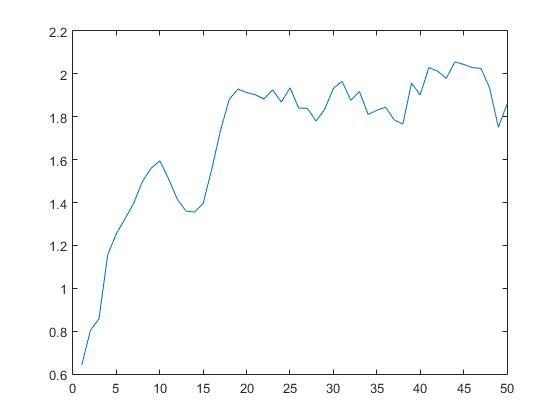
Figure 1: This image shows the mean fitness potential as a function of evolution time step. We observe an increase of the fitness

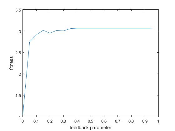
Figure 2: This plot shows the mean population fitness at the final evolution step as a function of the feedback parameter $r_{F}$. Note that for small $r_{F}$ the fitness does not reach maximum.

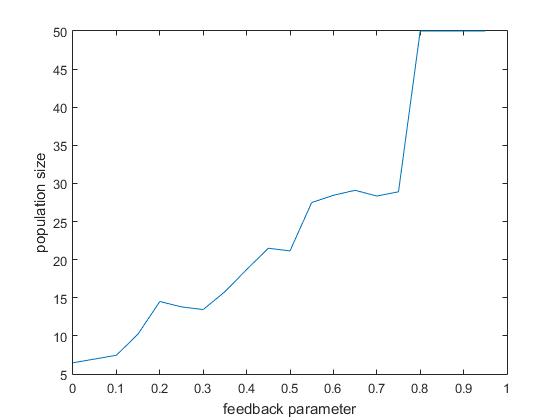
Figure 3: This plot shows the population abundance at the final evolution step as a function of the feedback parameter $r_{F}$. For small $r_{F}$ only a small part of organisms survive while for $r_{F}\approx 1$ all are viable.

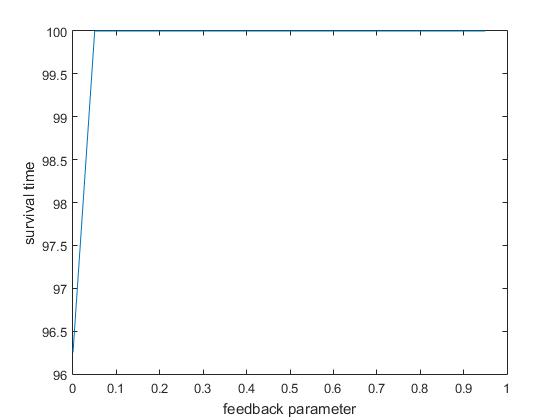
Figure 4: This plot shows the mean survival time as a function of the feedback parameter $r_{F}$. For small $r_{F}$ many populations extinct.

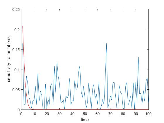
Figure 5: This plot shows two sensitivities as functions of time. The red curve shows sensitivity when the regulatory gene network canalizes evolution and $r_{F}=1$. The blue curve shows sensitivity when $r_{F}=0$ and the regulatory gene network is not involved in evolution. We see that the effect of gene regulation is very strong.

3.7.2 Simulations for different fitness functions

In the next series of simulations we consider fitness functions defined by $F=C_{M}\exp(\lambda W)$ with different potentials $W$. The main idea is to check a capacity of gene regulation to perform the fitness landscape learning even for very sophisticated fitness functions.

In all the cases (except for the Rosenberg function, see below) we use the simplest regulator described above and $C_{M}=5,\lambda=1$, $N_{\mathrm{popmax}}=100$ and $p_{\mathrm{mut}}=0.05$. In the canalized case the regulation parameter $r_{F}=1$, if canalization (regulation) is absent, we set $r_{F}=0$.

a ) Let $W$ be defined by (10) with $b_{i}=1$, $L=4$, and $\mu=5$, $m_{I}=2$. The results are shown on Fig. 1.

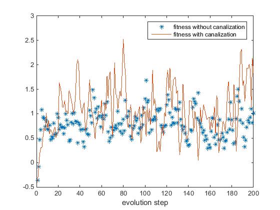
Figure 6: The case a). This plot shows that regulation with canalization increases the fitness. The fitness is shown in a logarithmic scale, i.e., the vertical axis shows the fitness potential $W$.

b ) In this case we set $W=\sum_{i=1}^{2}(z_{i}-1)^{2}+\sum_{i=3}^{6}z_{i}^{2}$. This function has a single maximum on the hypercube $[0,1]^{6}$ at $(0,0,1,1,1,1)$.

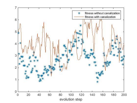
Figure 7: The case b). This plot shows how regulation with canalization increases the quadratic fitness with a single local maximum. The fitness is shown in a logarithmic scale, i.e., the vertical axis shows the fitness potential $W$.

c ) In this case we set $W=\sum_{i=1}^{6}b_{i}(z_{i}-1)^{2}+0.8b_{i}z_{i}^{2}$. This function has local maxima on the hypercube $[0,1]^{6}$ at the all hypercube vertices.

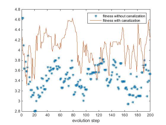
Figure 8: The case c). The fitness is shown in a logarithmic scale, i.e., the vertical axis shows the fitness potential $W$.

d) The quadratic fitness potential $W=\sum_{j=1}^{6}b_{j}*(z_{2j-1}+z_{2j}-2z_{2j-1}z_{2j})$, where there exist a number of local maxima.

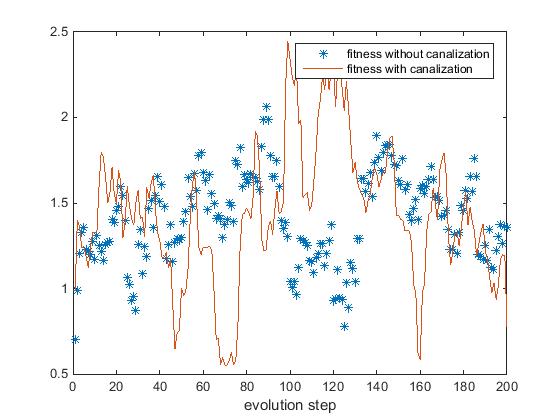
Figure 9: The case d)

e) Let us consider a special fitness, defined by the Rosenbrock function, which serves as a test for different optimization algorithms. The Rosenbrock function has the form

$$W=\sum_{j=1}^{m}(1-z_{j})^{2}+a(z_{j+1}-z_{j}^{2})^{2},$$

where $a>0$ is a large parameter. It is also known as Rosenbrock’s valley because the global minimum is inside a long, narrow, parabolic shaped valley. To find the valley, it is easy but to attain the global minimum, it is hard. Indeed, numerical simulations for $m=5$ and $a=10$ show that the fitness does attain the global maxima within a long evolution ($>200$ steps), in the both cases: without any regulation and with one described above in the beginning of this subsection. However, if we apply more sophisticated regulation defined by an analogue of the Hebb rule, we obtain a fast convergence to global maximum at $z=(1,1,1,1,1,1)$, see Fig. 5. So, we can go through valley by a gene learning organized by a Hebb’s like principle. How evolution can cross a fitness valley is an important question in genetics and it was considered by (Weissman et al. 2009).

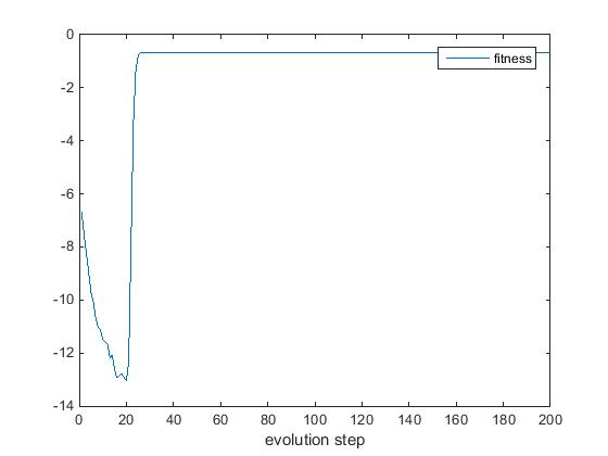
Figure 10: The case e. The fitness potential $W$ approaches to the global maximum for a hard test fitness function if evolution learning is organized in a special way. The fitness is shown in a logarithmic scale, i.e., the vertical axis shows the fitness potential $W$.

4 Conclusions and Discussion

The famous computer scientist Valiant (2013) wrote that evolutionary biology cannot explain the rate at which evolution occurs: “The evidence for Darwin’s general schema for evolution being essentially correct is convincing to the great majority of biologists. This author has been to enough natural history museums to be convinced himself. All this, however, does not mean the current theory of evolution is adequately explanatory. At present the theory of evolution can offer no account of the rate at which evolution progresses to develop complex mechanisms or to maintain them in changing environments.”

The first attempt to explain the fast evolution rate was made by Waddington (1942, 1953), who gave an idea of canalized evolution, however, without suggesting any mathematical models. Recently, however, some ideas and models were proposed by (Valiant 2006, 2009; Livnat et al. 2014; Parter et al. 2008), see also (Watson and Szathmáry 2015) for a review, in order to explain a possibility of adaptation with formation of many phenotypic traits. These models exploit basic Computer Science Theory approaches and methods to show that evolution can make a learning of fitness landscape that can accelerate evolution.

In this paper, we propose a model, which extends previous ones by Valiant (2006, 2009); Livnat et al. (2014); Parter et al. (2008) in two aspects. First, we use hybrid circuits involving two kinds of variables. The first class of variables are real valued ones, they range in the interval $[0,1]$ and they can be interpreted as relative levels of expression phenotypic traits or morphogene concentrations (morphogenes can make cell differentiation and thus change phenotypes). Other variables are Boolean and can be interpreted as genes. Second, we use a threshold scheme of regulation, which inspired by ideas of the paper by Stern (1958). All variables are involved in the gene regulation via thresholds. Our results are formulated in a mathematically rigorous form for such models, which involve general fitness functions and population dynamics, and which are based on fundamental biological ideas and experimentally confirmed facts. Namely, we assume that the multicellular organism phenotype depends on a number of phenotypical traits and these traits are completely determined by cell patterns. These patterns, in turn, are determined by expressions of special genes, for example, morphogenes. Expression of morphogenes is controlled by a number of other genes (genotype) and by network regulation loops that exploit threshold mechanisms and involve morphogenes and other genes. Populations are large but not obligatory infinite. The gene drift can be taken into account if it is small.

It is shown that our gene regulation scheme is powerful enough and allows to realize all possible feedback mechanisms, any algorithms of gene control (see Theorem I) and can produce any dynamics. So, such regulation scheme is powerful enough to realize any algorithms of evolution. We therefore essentially reinforce the results of Chastain et al. (2014), where it is shown that evolution can realize MWUA algorithms.

Furthermore, the gene regulation can perform fitness landscape recognition. According to our mathematical results it can be explained as follows. Consider a phenotypic trait, which is controlled, say, by many genes and by a threshold parameter. Suppose that for a fixed threshold we need 10 mutations to obtain expression level necessary for a good adaptation. Then in the classical mutation-selection scheme evolution uses approximately $p_{\mathrm{mut}}^{-10}$ generations.

The canalized evolution uses learning by gene network and it can work much faster. Indeed, it is sufficient to use only a single mutation. Suppose a mutation is happened, which affects the trait under consideration, and after $T_{c}\ll p_{\mathrm{mut}}^{-1}$ generations some progenies of that mutant are still viable. This fact on viability gives an information on the fitness landscape since it means that that change of the trait is useful for adaptation. Then the gene regulation network turns on making a change of the threshold. If after this change and new $T_{c}$ generations new progenies are still viable, then the gene regulation network make a new round of the threshold variation.

This capacity to fitness landscape recognition also explains results of Mitchell et al. (2009) on prediction of environmental changes. Moreover, gene network recognition strongly reduces the number of mutations that are necessary for adaptation because the gene regulatory networks reinforce effects of some mutations: a single mutation can lead to a large phenotype change, the fact, which is consistent with QTL date (Zeyl 2005).

So, learning based evolution can go faster since reduces need mutation number. However, this acceleration, based on stochastic learning algorithms, leads to an additional risk connected with learning errors. So, evolution reminds rates on a rugged highway: acceleration increases risk and finally, population can come to an evolution dead end. Actually, a biological uncertainty principle is obtained: to decrease the learning risk, evolution should use more test rounds and thus a smaller regulation parameter $r_{F}$, however, for smaller $r_{F}$ we obtain greater evolution times $T_{W}$.

Note that evolution as a learning problem was first considered in the pioneering paper by (Valiant 2006, 2009), where a formal Boolean circuit model is used. This model is essentially simpler and we think that it is less biologically realistic than the one considered here, since it does not involve genetic regular networks, which regulate Boolean circuits. The results obtained by (Valiant 2009) mean that evolution may be successful for a very narrow class of circuits. Opposite to (Valiant 2009) we conclude that evolution may be successful for a general class of the fitness functions due to genetic regulation. It is worth to note that these estimates of evolution acceleration can be done for random fitness landscapes. It is important fact since actually biologists know almost nothing about fitness landscapes for complex organisms (Franke et al. 2011).

We show that a learning by the regulatory gene networks also increases canalization, i.e., phenotype stability. Evolution, accelerated and canalized by evolution recognition procedures, becomes more irreversible. This fact yields important consequences for evolution in a varying environment. Learning by gene networks leads to canalization, however, this effect diminishes flexibility (evolvability). The fitness sensitivity with respect to mutations is a decreasing function of canalization level. A too strong canalization can become dangerous for population evolvability when environment changes.

This negative effect can be compensated by expression of other morphogenes or even a formation of new morphogenes. Then new structures result of old already preexisting ones. In this case evolution, as it was explained by Gould, can go by addition terminal. So, it is possible that the famous (although vague) idea, largely discussed beginning with 19-th century, that the morphogenesis recapitulates evolution, can be explained by the concept of canalized evolution.

Another possible mechanism to avoid negative consequences of canalization for varying environments can be connected with stress. It is well known and proved experimentally that under a stress (which can be induced by environmental factors, for example, temperature), gene and proteins that make genetic buffering (for example, shaperons such as Hsp90) change their activity that provoke mutations. However, the most of these mutations are negative and thus the mutants obtained by this way are not well adapted. Finally, results obtained in this paper support the idea of Waddington that, in a fixed environment, evolution acceleration and phenotype buffering are positively correlated effects. This correlation appears as a result of the fitness landscape learning by gene networks.

The case of varying environments needs an additional investigation and we plan to address it in a future work.

5 Appendix 1

Let us prove Theorem III.

First we formulate an auxiliary lemma, which gives an estimate of fluctuations of the number of progenies.

Lemma 1. Let $X(s,t)$ be the frequency of genotype $s$ at the moment $t$, $F(s)$ be the fitness of these individuals, and $\bar{F}(t)$ be the averaged population fitness at the moment $t$, and $\kappa=N_{pop}(t)^{-1/4}$. Then, if $p_{\mathrm{mut}}=0$, the frequency $X(s,t+1)$ at the moment $t+1$ lies in the interval

$$J=[X(s,t)F(s)\bar{F}(t)^{-1}(1-\kappa),\ X(s,t)\bar{F}(t)^{-1}(1+\kappa)]$$

with the probability $Pr_{t}$ satisfying estimate

$$Pr_{t}>P_{*},$$ (59)

where $P_{*}$ is defined by (40).

Proof. Recall that the number of progenies for each individual is defined by the Poisson law, this number has the average $F(s)/\bar{F}$ and the same variation. The number $N_{p}$ is thus a sum of identically distributed and independent random quantities. According to the Central Limit Theorem, for large $N_{s}$ the distribution of this sum is close to a normal one, with the average $N_{s}F(s)\bar{F}^{-1}$ and the same variation that gives (60) and completes the proof of Lemma.

Lemma 2. Let $p_{\mathrm{mut}}>0$ and (37) holds. Under assumptions of the previos Lemma, we have that the frequency $X(s,t+1)$ at the moment $t+1$ lies in the interval

$$J=[X(s,t)\eta_{1},\ X(s,t)\eta_{2}],$$

where

$$\eta_{1}=(F(s)\bar{F}(t)^{-1}(1-\kappa)-2p_{\mathrm{mut}}),$$

$$\eta_{2}=(F(s)\bar{F}(t)^{-1}(1+\kappa)+(N_{popmax}p_{\mathrm{mut}})(X(s,t)N_{popmin})^{-1}$$

with the probability $\tilde{P}r_{t}$ satisfying estimate

$$Pr_{t}>(1-4P_{*}p_{m}),$$ (60)

where $p_{m}$ is defined by (37).

Proof. The proof uses the same arguments as above in the previous lemma. Let us take into account mutations. The frequency $X(s^{\prime},t)$ can be increased as a result of mutations in all the rest genotypes. The averaged number $N_{mut}$ of such mutants is $E_{m}=N_{pop}(t)p_{\mathrm{mut}}\ll 1$, where $N_{\mathrm{pop}}(t)\in[N_{\mathrm{popmin}},N_{popmax}]$. Under condition (37) the number $N_{\mathrm{mut}}$ is a random quantity subject to the Poisson law with the mean $E_{m}$ and the same variation. The probability that there will be at least one mutant is less than $2p_{m}$. These arguments give the right bound of $\eta_{2}$ for the interval $J$.

Similarly, we can find an estimate from below for $X(s,t)$ and it gives us the left bound of $J$ that proves the lemma.

Proof of Theorem.

We use Lemma 2 and repeat the proof of Theorem II with small modifications. Let us introduce the quantities

$$Q(t)=\frac{X(s,t)}{X(s^{\prime},t)}.$$

Then, by applying the lemma 2 step by step, we obtain that the following inequality

$$Q(T_{c}+T_{1})>Q(T_{1})(\frac{\eta_{1}}{\eta_{2}}^{T_{c}},$$

which holds with the probablity $(1-4P_{*}p_{m})^{T_{c}}$. Now repeating the proof of Theorem II, we obtain the conclusion of the Theorem III.

6 Appendix 2

The main idea of the proof is to represent the characteristic functions $\chi_{W(z^{\prime})-W(z)>0}(b)$ by the Fourier integrals as follows:

$$\chi_{W(z^{1})>W(z^{0})}=\int_{0}^{+\infty}\mathrm{d}x\int_{-\infty}^{+\infty}\exp(it(W(z^{1},b)-W(z^{0},b)-x))\mathrm{d}t,$$ (61)

where $i=\sqrt{-1}$. We set $\psi(z^{0},z^{1})=\psi^{1}=W(z^{1})-W(z^{0})$ and $\psi(z^{*},z^{1})=\psi^{2}=W(z^{*})-W(z^{1})$. These functions can be represented as

$$\psi^{1}=\sum_{k}b_{k}\psi_{k}^{0},\quad\psi^{2}=\sum_{k}b_{k}\psi_{k}^{1}.$$

Therefore,

$$\begin{array}[]{l}\mathrm{Pr}(Y_{0}Y_{1})=\\ \int_{0}^{+\infty}\int_{0}^{+\infty}\mathrm{d}x_{1}\mathrm{d}x_{2}\int_{-\infty}^{+\infty}\int_{-\infty}^{+\infty}\mathrm{d}t_{1}\mathrm{d}t_{2}\int_{{\bf R}^{N_{b}}}\exp(iS)\mathrm{d}\mu,\end{array}$$ (62)

where $S=t_{1}(\psi^{1}-x_{1})+it_{2}(\psi^{2}-x_{2})$.

The functions $\psi^{l}$ are linear in the variables $b_{j}$. Thus the integrals over $b_{i}$ have the form of typical Gaussian ones. We compute these integrals that gives

$$\begin{array}[]{l}\mathrm{Pr}(Y_{1}Y_{0})=\\ C^{-1}\int_{0}^{+\infty}\int_{0}^{+\infty}\mathrm{d}x_{1}\mathrm{d}x_{2}\int_{-\infty}^{+\infty}\int_{-\infty}^{+\infty}\exp(\Phi)\mathrm{d}t_{1}\mathrm{d}t_{2},\end{array}$$ (63)

where

$$\Phi=-\frac{(t_{1}\psi^{1}+t_{2}\psi^{2})^{2}}{4}+it_{1}x_{1}+it_{2}x_{2}.$$

and the normalizing factor $C$ can be written in an analogous form:

$$C=\int_{-\infty}^{+\infty}\int_{-\infty}^{+\infty}\mathrm{d}x_{1}\mathrm{d}x_{2}\int_{-\infty}^{+\infty}\int_{-\infty}^{+\infty}\exp(\Phi)\mathrm{d}t_{1}\mathrm{d}t_{2}.$$ (64)

According to (44) one has

$$\Phi=-(a_{00}t_{1}^{2}+a_{11}t_{2}^{2}+2a_{01}t_{1}t_{2})/4+it_{1}x_{1}+it_{2}x_{2}.$$

Now we compute the integrals (63) and (64) over $t_{1}$ and then over $t_{2}$, which also are Gaussian ones. We obtain

$$\begin{array}[]{l}\mathrm{Pr}(Y_{0}Y_{1})=\\ C^{-1}\int_{0}^{+\infty}\int_{0}^{+\infty}\exp(-\frac{x_{1}^{2}+r^{-2}(x_{2}a_{00}-x_{1}a_{01})^{2}}{4a_{00}})\mathrm{d}x_{1}\mathrm{d}x_{2},\end{array}$$

where $r^{2}=a_{00}a_{11}-a_{01}^{2}$, and

$$C=\int_{-\infty}^{+\infty}\int_{-\infty}^{+\infty}\exp(-\frac{x_{1}^{2}+r^{-2}(x_{2}a_{00}-x_{1}a_{01})^{2}}{4})\mathrm{d}x_{1}\mathrm{d}x_{2}.$$

In the both integrals we make the changes of variables, first $x_{1},x_{2}\to x_{1},w=x_{2}a_{00}-x_{1}a_{01}$ and then $x_{1}=u\sqrt{a_{00}},\ w=v\sqrt{a_{00}}r$. Finally, this procedure gives relation (47).

References

- Aita et al. (2001) Aita, T., M. Iwakura, and Y. Husimi, 2001 A cross-section of the fitness landscape of dihydrofolate reductase. Protein Eng. 14: 633–638.
- Arora et al. (2012) Arora, S., E. Hazan, and S. Kale, 2012 The Multiplicative Weights Update Method: A Meta-Algorithm and Applications. Theory Comput. 8: 121–164.
- Barron (1993) Barron, A. R., 1993 Universal approximation bounds for superposition of a sigmoid function. IEEE Trans. Inf. Theory 39: 930–945.
- Chastain et al. (2014) Chastain, E., A. Livnat, C. Papadimitriou, and U. Vazirani, 2014 Algorithms, games, and evolution. Proc. Natl. Acad. Sci. U. S. A. pp. 1–4.
- Cook (1971) Cook, S. A., 1971 The complexity of theorem-proving procedures. In Proc. third Annu. ACM Symp. Theory Comput. – STOC ’71, pp. 151–158, New York, New York, USA, ACM Press.
- Franke et al. (2011) Franke, J., A. Klözer, J. A. G. M. de Visser, and J. Krug, 2011 Evolutionary accessibility of mutational pathways. PLoS Comput. Biol. 7.
- Friedgut (1999) Friedgut, E., 1999 Sharp thresholds of graph properties, and the -sat problem. J. Am. Math. Soc. 12: 1017–1055.
- Grigoriev et al. (2014) Grigoriev, D., J. Reinitz, S. Vakulenko, and A. Weber, 2014 Punctuated evolution and robustness in morphogenesis. Biosystems 123: 106–113.
- Hopfield (1982) Hopfield, J. J., 1982 Neural networks and physical systems with emergent collective computational abilities. Proc. Natl. Acad. Sci. 79: 2554–2558.
- Kauffman and Weinberger (1989) Kauffman, S. A. and E. D. Weinberger, 1989 The NK model of rugged fitness landscapes and its application to maturation of the immune response. J. Theor. Biol. 141: 211–245.
- Kingman (1978) Kingman, J. F. C., 1978 A simple model for the balance between selection and mutation. J. Appl. Probab. 15: 1–12.
- Levin (1973) Levin, L. A., 1973 Universal enumeration problems (russian). Probl. Peredai Inf. 9: 115116.
- Livnat et al. (2014) Livnat, A., C. Papadimitriou, A. Rubinstein, G. Valiant, and A. Wan, 2014 Satisfiability and evolution. In Annu. IEEE Symp. Found. Comput. Sci. FOCS, pp. 524–530.
- Masel and Siegal (2009) Masel, J. and M. L. Siegal, 2009 Robustness: mechanisms and consequences. Trends Genet. 25: 395–403.
- Mitchell et al. (2009) Mitchell, A., G. H. Romano, B. Groisman, A. Yona, E. Dekel, M. Kupiec, O. Dahan, and Y. Pilpel, 2009 Adaptive prediction of environmental changes by microorganisms. Nature 460: 220–4.
- Mjolsness et al. (1991) Mjolsness, E., D. H. Sharp, and J. Reinitz, 1991 A connectionist model of development. J. Theor. Biol. 152: 429–453.
- Moore and Mertens (2011) Moore, C. and S. Mertens, 2011 The Nature of Computation. Oxford University Press.
- Mukherji et al. (2011) Mukherji, S., M. S. Ebert, G. X. Y. Zheng, J. S. Tsang, P. A. Sharp, and A. van Oudenaarden, 2011 MicroRNAs can generate thresholds in target gene expression. Nat. Genet. 43: 854–9.
- Nagylaki (1993) Nagylaki, T., 1993 The evolution of multilocus systems under weak selection. Genetics 134: 627–647.
- Orr (2005) Orr, H. A., 2005 The genetic theory of adaptation: a brief history. Nat. Rev. Genet. 6: 119–127.
- Parter et al. (2008) Parter, M., N. Kashtan, and U. Alon, 2008 Facilitated variation: How evolution learns from past environments to generalize to new environments. PLoS Comput. Biol. 4.
- Rutherford and Lindquist (1998) Rutherford, S. L. and S. Lindquist, 1998 Hsp90 as a capacitor for morphological evolution. Nature 396: 336–342.
- Stern (1958) Stern, C., 1958 Selection for subthreshold differences and the origin of pseudoexogenous adaptations.
- Valiant (2013) Valiant, L., 2013 Probably Approximately Correct: Nature’s Algorithms for Learning and Prospering in a Complex World. Basic Books.
- Valiant (2006) Valiant, L. G., 2006 Evolvability. Technical Report 120.
- Valiant (2009) Valiant, L. G., 2009 Evolvability. J. ACM 56: 1–21.
- Waddington (1953) Waddington, C., 1953 Genetic assimilation of an acquired character. Evolution 7: 118–126.
- Waddington (1942) Waddington, C. H., 1942 Canalization of development and the inheritance of acquired characters. Nature 150: 563–565.
- Watson and Szathmáry (2015) Watson, R. A. and E. Szathmáry, 2015 How can evolution learn? Trends Ecol. Evol. pp. 1–11.
- Weissman et al. (2009) Weissman, D. B., M. M. Desai, D. S. Fisher, and M. W. Feldman, 2009 The rate at which asexual populations cross fitness valleys. Theor. Popul. Biol. 75: 286–300.
- Zeyl (2005) Zeyl, C., 2005 The number of mutations selected during adaptation in a laboratory population of Saccharomyces cerevisiae. Genetics 169: 1825–1831.