Surprises from quenches in long-range interacting systems: Temperature inversion and cooling

Abstract

What happens when one of the parameters governing the dynamics of a long-range interacting system of particles in thermal equilibrium is abruptly changed (quenched) to a different value? While a short-range system, under the same conditions, will relax in time to a new thermal equilibrium with a uniform temperature across the system, a long-range system shows a fast relaxation to a nonequilibrium quasistationary state (QSS). The lifetime of such an off-equilibrium state diverges with the system size, and the temperature is non-uniform across the system. Quite surprisingly, the density profile in the QSS obtained after the quench is anticorrelated with the temperature profile in space, thus exhibiting the phenomenon of temperature inversion: denser regions are colder than sparser ones. We illustrate with extensive molecular dynamics simulations the ubiquity of this scenario in a prototypical long-range interacting system subject to a variety of quenching protocols, and in a model that mimics an experimental setup of atoms interacting with light in an optical cavity. We further demonstrate how a procedure of iterative quenching combined with filtering out the high-energy particles in the system may be employed to cool the system. Temperature inversion is observed in nature in some astrophysical settings; our results imply that such a phenomenon should be observable, and could even be exploitable to advantage, also in controlled laboratory experiments.

Keywords: Long-range interactions, Vlasov equation, Quasi-stationary states, Temperature inversion

1 Introduction

Long-range-interacting systems abound in nature [1, 2, 3]. Interactions are called long-range when the pair potential energy decays asymptotically with the interparticle distance $r$ as $r^{-\alpha}$, with $0\leq\alpha\leq d$ in $d$ spatial dimensions, as it happens for instance in Coulomb and gravitational interactions. One striking feature of many-particle long-range interacting systems is that they are typically found in states that are out of thermodynamic equilibrium. This is at variance with systems with short-range interactions: while nonequilibrium states in short-range systems require an enduring external forcing to counteract the tendency of the system to reach due to “collisional” effects a thermal equilibrium state, an isolated long-range interacting system evolving while starting far from equilibrium will remain stuck in an out-of-equilibrium state for very long times. Such times grow with the number $N$ of degrees of freedom, so that they may become larger than any experimentally accessible timescale. For instance, the time needed for a galaxy to reach an “equilibrium” state is estimated to be several orders of magnitude larger than the age of the universe [4, 5]. This property is universal, in the sense that it is shared by all systems with long-range interactions, regardless of the details of the interaction potential . It is understood as a consequence of the fact that the kinetic equation governing the evolution of the single-particle distribution function $f(\mathbf{q},\mathbf{p},t)$, where $\mathbf{q}$ and $\mathbf{p}$ are the canonically conjugated positions and momenta, respectively, is the Vlasov equation (often referred to as the collisionless Boltzmann equation, mainly in the astrophysical literature), up to a timescale $\tau_{\mathrm{coll}}$ when collisional effects can no longer be neglected, with $\tau_{\mathrm{coll}}$ diverging with $N$ [1, 3]. Such an equation has infinitely many stationary solutions: among these, the stable ones are identified with the observed non-equilibrium states, often referred to as quasi-stationary states (QSSs), and the thermal equilibrium state is just one out of infinitely many.

The overall qualitative picture of the dynamical evolution of an isolated long-range system starting far from thermal equilibrium is the following: After a transient (referred to as violent relaxation after Lynden-Bell [6]) whose lifetime does not depend on $N$, the system sets into a QSS and stays there for a time of the order of $\tau_{\mathrm{coll}}$. For times $t>\tau_{\mathrm{coll}}$, when the Vlasov description no longer applies, the QSS is no longer stationary, and the system eventually evolves to a thermal equilibrium state. The QSS the system relaxes to after the violent relaxation depends on the initial conditions, and no general theory is available yet to predict it. A completely general statistical approach was proposed by Lynden-Bell [6], but it rests on the hypothesis of complete mixing of the Vlasov dynamics that only rarely holds, hence, gives reasonably accurate predictions only in very particular cases [3, 7]. Other methods have been proposed since then, which give good predictions for simple models only for special classes of initial conditions, namely, for single-level initial distributions (the so-called “water-bag” distributions) [3, 7] or when the relaxation towards the QSS is nearly adiabatic [7, 8, 9, 10].

Although predicting the full distribution function in a QSS resulting from a generic initial condition is a formidable task, especially for spatially inhomogeneous QSSs whose stability properties are particularly difficult to analyze, one may ask whether the QSSs that are reached in certain situations do share some common features. One of the hallmarks of thermal equilibrium is a uniform temperature throughout the system, hence, also in inhomogeneous equilibrium states, the temperature will be constant. Conversely, in a nonequilibrium state, the temperature may well be nonuniform. Hence, one may ask whether some properties of the temperature profile in a QSS share a certain degree of universality. A physically relevant case is that of a system prepared in a (spatially inhomogeneous) thermal equilibrium state and then brought out of equilibrium by means of a (non-small) sudden perturbation, acting for a very short time. As shown in recent papers [11, 12], in this case, the typical outcome is somewhat surprising and counterintuitive, and is referred to as temperature inversion. The latter effect implies that the density and temperature profiles are anticorrelated: sparser regions of the system are hotter than denser ones. Temperature inversions are observed in nature in astrophysical settings, the most famous example being the solar corona, where the temperature grows from thousands to millions of Kelvin while going from the photosphere to the sparser external regions of the corona [13]. Other examples of temperature inversions have been observed, for instance, in molecular clouds [14]. As argued in [11, 12, 15], temperature inversion should not be a peculiarity of systems in extreme conditions, as astrophysical systems typically are, but should rather be a generic property of long-range interacting systems relaxing to a QSS after having been brought out of (spatially inhomogeneous) thermal equilibrium by a perturbation. In [11], temperature inversion was observed as a result of perturbations of a thermal state of a prototypical model with long-range interactions, the Hamiltonian mean-field (HMF) model [16], and of a two-dimensional self-gravitating system. Temperature inversion in the latter system is thoroughly investigated in [17] in connection with filamentary structures in galactic molecular clouds. Partial temperature inversions were also observed in QSSs of two-dimensional self-gravitating systems whose initial conditions were of the water-bag type [18]. In one-dimensional self-gravitating systems, temperature inversions in QSSs were observed, which gradually disappear during the slow relaxation of the system from the QSS to thermal equilibrium [19]. Temperature inversion was recently demonstrated to occur in the nonequilibrium stationary state of a class of mean-field systems involving rotators subject to quenched disordered external drive and dissipation [20]. A physical picture of the origin of temperature inversion in a generic long-range interacting system, based on the interplay between a mechanism originally proposed to explain the temperature profile in the solar corona (referred to as velocity filtration [21, 22, 23, 24]) and the interaction of the system particles with the time-dependent mean field, was also suggested [11].

If the phenomenon of temperature inversion is somewhat universal in long-range interacting systems abruptly brought out of thermal equilibrium, one may wonder whether it could be observed also in a controlled laboratory experiment. In the present paper, we aim at taking a step forward towards a positive answer to this question. First of all, using molecular dynamics (MD) simulations, we demonstrate that in the HMF model, with both attractive and repulsive interactions, temperature inversion is typically observed when the system is brought out of thermal equilibrium by means of an abrupt change (from now on referred to as a quench) of a parameter controlling the dynamics of the system, like a coupling constant or an external field. To this end, we employ a variety of different quench protocols. Our studies are relevant to experiments because quench protocols can be performed with experimental setups, especially in systems of (cold) atoms; moreover, an HMF model with repulsive interactions and an external confining field can be seen as a toy model of trapped ions, while an HMF model with attractive interactions does share many features with atoms interacting with light in a cavity. We then elaborate on this point by demonstrating that at least one of the considered quench protocols can be applied to another model, which mimics more closely an experimental setup of atoms interacting with a standing electromagnetic wave in an optical cavity [25, 26, 27], again yielding temperature inversion. It is worth noting that the quenching protocol applicable to the latter model does correspond to changing a parameter that can be actually tuned in an experiment, that is, the intensity of an external laser pump. We also give evidence that the physical picture proposed in [11] does apply to temperature inversions produced by quenches. Finally, we show that an iterative quenching protocol, combined with filtering out the high-energy particles localized in the sparser external regions, can be used to cool the system.

The paper is organized as follows: in Sec. 2, we introduce the HMF model, and study the temperature inversion produced by quenching the external field in the case of repulsive interactions (§2.1.1) as well as that produced in the case with attractive interactions by quenching the external field (§2.2.1) and the coupling constant (§2.2.2). In Sec. 3, we discuss a model of atoms interacting with light in an optical cavity, with emphasis on the dissipationless limit (§3.1). We then report on temperature inversion as observed in the latter system after quenching the coupling constant (§3.1.1), and discuss its possible observation in a laboratory experiment (§3.1.2). Section 4 is devoted to demonstrating that an iterative application of the previously considered quenching protocols can cool the systems. Finally, conclusions are drawn and open issues are discussed in Sec. 5.

2 Temperature inversion in the Hamiltonian mean-field (HMF) model

The prototypical model of long-range interacting systems that we shall consider in this paper is the so-called Hamiltonian mean field (HMF) model [16]. The model comprises a system of $N$ globally-coupled point particles of unit mass moving on a circle. The Hamiltonian of the system, in presence of an external field of strength $h$, is given by

$$H=\sum_{i=1}^{N}\frac{p_{i}^{2}}{2}+\frac{J}{2N}\sum_{i,j=1}^{N}[1-\cos(\vartheta_{i}-\vartheta_{j})]-h\sum_{i=1}^{N}\cos\vartheta_{i}.$$ (1)

Here, $\vartheta_{i}\in[-\pi,\pi]$ is the angular coordinate of the $i$-th particle $(i=1,2,\ldots,N)$ on the circle, while $p_{i}$ is the conjugated momentum, see Fig. 1(a). The coupling constant $J$ can be either positive or negative, defining respectively the ferromagnetic (F) and the antiferromagnetic (AF) version of the model. The reason for the use of terms borrowed from the physics of magnetic systems is that the HMF model can also be seen as a system of planar ($XY$) spins with mean-field couplings (that is, defined on a complete graph with links of the same strength). For $h=0$, therefore, the Hamiltonian (1) is $O(2)$-invariant. Ferromagnetic (respectively, antiferromagnetic) interactions in the magnetic picture correspond to attractive (respectively, repulsive) interactions in the particle interpretation. The time evolution of the system is governed by the Hamilton equations derived from the Hamiltonian (1):

$$\left\{\begin{array}[]{ccl}{\displaystyle\frac{{\rm d}\vartheta_{i}}{{\rm d}t}}&=&p_{i}\,,\\ &&\\ {\displaystyle\frac{{\rm d}p_{i}}{{\rm d}t}}&=&J(m_{y}\cos\vartheta_{i}-m_{x}\sin\vartheta_{i})-h\sin\vartheta_{i}\,,\end{array}\right.$$ (2)

where $(m_{x},m_{y})\equiv(1/N)\sum_{i=1}^{N}(\cos\vartheta_{i},\sin\vartheta_{i})$ are the components of the magnetization vector ${\bf m}\equiv(m_{x},m_{y})$, whose magnitude $m\equiv\sqrt{m_{x}^{2}+m_{y}^{2}}$ measures the amount of clustering of particles on the circle. A uniform (respectively, non-uniform) distribution of particles on the circle implies the value $m=0$ (respectively, $m\neq 0$).

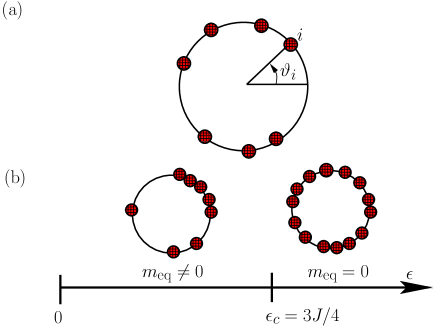
Figure 1: (a) Schematic diagram of the Hamiltonian mean-field (HMF) model; the $i$-th particle is characterized by the angular coordinate $\vartheta_{i}$ and conjugate momentum $p_{i}$. (b) Equilibrium phase diagram of the F-HMF model in the absence of the external field $h$: As a function of the energy density $\varepsilon$, a continuous transition between a magnetized ($m_{\rm eq}\neq 0$) and a non-magnetized ($m_{\rm eq}=0$) state occurs at the critical value $\varepsilon_{c}=3J/4$.

Let us denote by $f(\vartheta,p,t)$ the time-dependent single-particle distribution function, which is the probability density to have a particle with angular coordinate $\vartheta$ and momentum $p$ at time $t$. In thermal equilibrium at temperature $T$, the distribution has the form [3]

$$f_{\rm eq}(\vartheta,p)\propto\exp\left\{-\frac{1}{T}\left[\frac{p^{2}}{2}-J\left(m_{x}^{\rm eq}\cos\vartheta+m_{y}^{\rm eq}\sin\vartheta\right)-h\cos\vartheta\right]\right\},$$ (3)

where the equilibrium magnetization components are obtained self-consistently as $(m_{x}^{\rm eq},m_{y}^{\rm eq})\equiv\int{\rm d}\vartheta{\rm d}p\,(\cos\vartheta,\sin\vartheta)f_{\rm eq}(\vartheta,p)$. In Eq. (3), we have set the Boltzmann constant to unity, as we shall do throughout the paper. In the special case $m_{y}^{\rm eq}=0$, that is, for distribution of particles symmetric around $\vartheta=0$ that we shall focus on in the following, the self-consistent relation for the magnetization may be written as [1, 3]

$$m_{\rm eq}=\frac{I_{1}\left[\beta(Jm_{\rm eq}+h)\right]}{I_{0}\left[\beta(Jm_{\rm eq}+h)\right]}~{},$$ (4)

where $m_{\rm eq}\equiv m_{x}^{\rm eq},\beta=T^{-1}$, and $I_{n}(x)$ denotes the modified Bessel function of order $n$. For $h\neq 0$, the system in thermal equilibrium is characterized by an inhomogeneous distribution of particles on the circle, with clustering around $\vartheta=0$. In the AF case, a nonzero external field is necessary to have an inhomogeneous thermal state, while in the F case, a clustered equilibrium state is attained even with $h=0$, via a spontaneous breaking of the $O(2)$ symmetry by the attractive interaction between the particles, provided the total energy density is smaller than a critical value $\varepsilon_{c}\equiv 3J/4$, see Fig. 1(b); the corresponding critical temperature is $T_{c}\equiv J/2$ [1, 3]. The F-HMF system with $h=0$ in fact shows a continuous phase transition as a function of temperature, with $m_{\rm eq}$ decreasing continuously from unity at $T=0$ to zero at $T=T_{c}$, while remaining zero at higher temperatures [1, 3].

Let us note that the Hamiltonian (1) can be obtained by taking any long-range interacting system, restricting to one spatial dimension, expanding the potential energy in a Fourier series, and retaining just the first Fourier mode [7, 11]. The AF-HMF model can be seen to represent a one-component Coulomb system, while the F-HMF is a simplified description of a self-gravitating system. As anticipated in the Introduction, and as we shall see further in Sec. 3, the F-HMF model turns out to be very closely related to a different system, i.e., a system of atoms in an optical cavity.

2.1 The antiferromagnetic case

Let us now discuss how quenching one of the parameters of the Hamiltonian (1) when the system is in an inhomogeneous thermal equilibrium state produces a non-equilibrium state exhibiting temperature inversion. To start with, we consider the AF case with $h\not=0$.

2.1.1 Quenching the external field

We consider $N=10^{6}$ particles and prepare the system in an inhomogeneous equilibrium state ($m_{\rm eq}\neq 0$) at an initial value of the field $h=15$ and temperature $T=5$, by sampling independently for every particle the coordinate $\vartheta$ and the momentum $p$ from the distribution (3). We take the coupling to be $J=-1$. In such a state, while the local density $n(\vartheta)$, defined as

$$n(\vartheta)\equiv\int{\rm d}p\,f(\vartheta,p,t)\,,$$ (5)

is non-uniform, corresponding to a magnetization $m_{\rm eq}\approx 0.797$, the local temperature, defined as

$$T(\vartheta)\equiv\frac{\int{\rm d}p\,p^{2}f(\vartheta,p,t)}{n(\vartheta)}\,,$$ (6)

is nevertheless uniform as a function of $\vartheta$. We study the time evolution of the system starting from this equilibrium state by performing a MD simulation that involves integrating the equations of motion (2). At $t=100$, we instantaneously quench the field to $h=10$. Soon after the quench, the magnetization of the system starts oscillating; the oscillations damp out in time, and eventually the system relaxes to a QSS with $m_{\rm QSS}<m_{\rm eq}$ at the new value of the field. The latter fact is expected since the value of $h$ is smaller than in the initial state. The time evolution of the magnetization for a time window around the time of the quench is shown in Fig. 2.

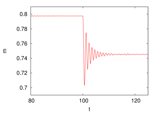
Figure 2: AF-HMF model in presence of an external field. Time evolution of the magnetization $m$: Starting with thermal equilibrium (3) at temperature $T=5$ and field $h=15$, the field strength is instantaneously quenched at $t=100$ to $h=10$. The number of particles is $N=10^{6}$, and the coupling constant is $J=-1$.

For times larger than those shown in Fig. 2, the magnetization stays essentially constant with extremely small fluctuations, signaling that the system has relaxed to a QSS. The density and temperature profiles as a function of $\vartheta$ in the QSS are plotted in Fig. 3. It is apparent that $n(\vartheta)$ and $T(\vartheta)$ are anticorrelated. The system exhibits a clear temperature inversion: denser regions are colder than sparser ones. We note that the average temperature

$$\langle T\rangle\equiv\int{\rm d}\vartheta\,T(\vartheta)n(\vartheta)$$ (7)

has the value $\langle T\rangle\approx 4$ in the QSS, lower than the initial value $T=5$. We shall come back to this point in §4.

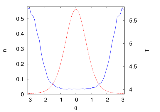
Figure 3: Temperature inversion in the AF-HMF model after a quench of the external field. Local density $n$ (red dot-dashed line) and local temperature $T$ (blue solid line) measured at $t=10^{3}$ in the QSS obtained under the same conditions as for Fig. 2.

Apart from the reduction of the average temperature, these results are qualitatively very similar to those obtained in [11] for a ferromagnetic HMF model. In that work, however, the simulation protocol was different, because the system was initiated in equilibrium with $h=0$ and then an external field was applied for a very short time. In Ref. [11], a physical picture was put forward to explain the emergence of temperature inversion, and we argue that it applies also in the present case (and, as we shall discuss below, to all the cases discussed in the present paper). Without entering into details, let us recall the main points of this explanation. After the quench (or the perturbation), a collective oscillation (i.e., a wave) sets in, as witnessed by the time evolution of the magnetization (Fig. 2). The oscillation damps out in time, but the system is conservative with no dissipative mechanism being present. Hence, the energy lost by the wave must be acquired by some of the particles. This may happen via Landau damping, an ubiquitous phenomenon in systems with long-range interactions: particles whose velocity is not too far from the phase velocity $v_{\rm ph}$ of the wave interact strongly with the wave itself. The net result is that the nearly resonant particles gain kinetic energy from the wave, so that the momentum distribution $f(p)\equiv\int{\rm d}\vartheta f(\vartheta,p)$ develops small peaks or shoulders and becomes different from a thermal distribution. In particular, close to the resonances, there will be suprathermal regions, i.e., regions where $f(p)$ is larger than the initial thermal distribution. Now, the mechanism of velocity filtration comes into play as follows. The density $n(\vartheta)$ is maximum at $\vartheta=0$ and decreases for larger and smaller $\vartheta$’s, reaching its minimum around $\vartheta=\pm\pi$. The net effect of the interaction between the particles and the external field is to create an effective force field pushing the particles towards $\vartheta=0$, so that the particles have to climb the potential energy well to reach the sparser regions of the system; particles with larger kinetic energies will do that more easily than “colder” particles, and any suprathermal region present in the velocity distribution will be magnified in regions where the particle density is lower. This is precisely what happens in our case, as shown in Fig. 4, where the velocity distribution function measured at a position where the particle density $n$ is smaller, $f(\vartheta=\pi,p)$, see panel (a), is plotted together with the same function measured at the position of maximum density, $f(\vartheta=0,p)$, see panel (b). Magnified suprathermal regions in $f(\vartheta=\pi,p)$ are apparent, and are responsible for the fact that the variance of the velocity distribution is here larger than in the denser regions of the system.

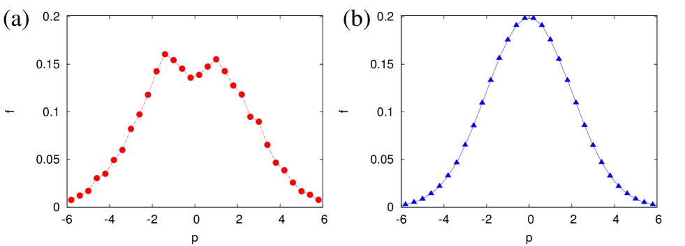
Figure 4: Momentum distribution of the AF-HMF model measured at $t=10^{3}$ in the QSS obtained under the same conditions as for Fig. 2. (a) The distribution at $\vartheta=\pi$ at which the density is minimum. (b) The distribution at $\vartheta=0$ at which the density is maximum.

We performed other numerical experiments with the same quench protocol by varying the initial temperature and the difference between the initial and final values of the field $h$, and obtained qualitatively similar results. No fine-tuning of the parameters is necessary to observe temperature inversion. We repeated some of the numerical experiments with $N=10^{7}$ particles, observing no differences with respect to the $N=10^{6}$ case.

In principle, one can quench also the coupling constant $J$, while keeping the field $h$ fixed. However, as stated before, as far as laboratory systems are concerned, the AF-HMF system can be seen as a toy model of a system of equal electric charges in a confining field, i.e., ions in a trap. In trapped ions, quenching $h$ corresponds to quenching the strength of the confining trap, which in principle is an experimentally feasible protocol. Conversely, quenching $J$ is equivalent to quenching the charge of the ions, which does not seem very physical, so that we do not study this kind of quench protocol for the AF case.

2.2 The ferromagnetic case

Let us now turn to the ferromagnetic (F-HMF) case, that is, $J>0$. Without loss of generality, we take the coupling to be $J=1$.

2.2.1 Quenching the external field

We repeat for the F-HMF system the numerical experiment we performed with the AF system. We prepare the system of $N=10^{6}$ particles in inhomogeneous thermal equilibrium at temperature $T=5$ and with a field $h=15$, now corresponding to $m_{\rm eq}\approx 0.821$, and evolve the system up to $t=100$, when we quench the external field to $h=10$. As in the AF case, the magnetization starts oscillating (Fig. 5), the oscillation damps out in time, and the system settles in a QSS with temperature inversion (Fig. 6).

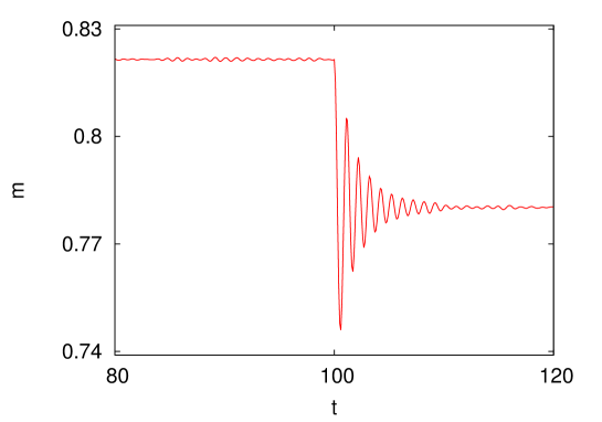
Figure 5: F-HMF model in presence of an external field. Time evolution of the magnetization $m$: Starting with thermal equilibrium (3) at temperature $T=5$ and field $h=15$, the field is instantaneously quenched at $t=100$ to $h=10$. The number of particles is $N=10^{6}$, and the coupling constant is $J=1$.

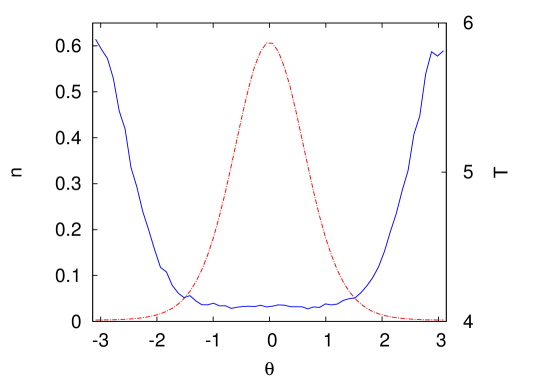
Figure 6: Temperature inversion in the F-HMF model after a quench of the external field. Local density $n$ (red dot-dashed line) and local temperature $T$ (blue solid line) measured at $t=10^{3}$ in the QSS obtained under the same conditions as for Fig. 5.

Figures 5 and 6 are very similar to the corresponding ones for the AF system, that is, Figs. 2 and 3, respectively. The same is true for the momentum distributions, shown in Fig. 7, which is strikingly similar to Fig. 4.

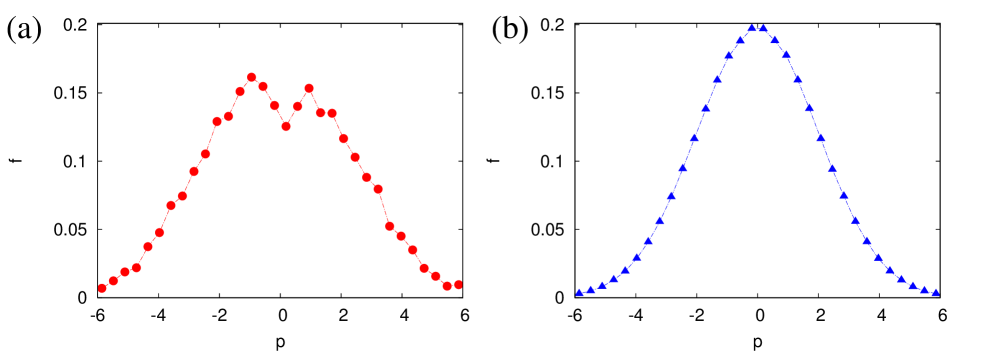
Figure 7: Momentum distribution of the F-HMF model measured at $t=10^{3}$ in the QSS obtained under the same conditions as for Fig. 5. (a) The distribution at $\vartheta=\pi$ at which the density is minimum. (b) The distribution at $\vartheta=0$ at which the density is maximum.

Hence, also in this case, the physical picture based on wave-particle interaction and velocity filtration applies. Consistent with our physical picture, the sign of the interactions is irrelevant for field quenches, as long as the field is sufficiently strong to produce the dominant effects of shaping the density profile $n(\vartheta)$ and providing the effective potential well that filters the velocities of the particles, thereby producing temperature inversion. Again, we repeated our numerical experiments for different values of the fields, for different initial temperatures and for systems with $N=10^{7}$, observing no qualitative differences. We note that similar to the AF case, the average temperature in the QSS for the F case is smaller than the initial temperature, and one has $\langle T\rangle\approx 4$.

2.2.2 Quenching the coupling constant

As we have previously discussed, the F-HMF model admits magnetized (collapsed) thermal equilibrium states also for $h=0$, provided $T<J/2$. Moreover, as we shall see in Sec. 3, the F-HMF model also admits an interpretation in terms of an atomic system, where the coupling constant $J$ is tunable in an experiment. We thus turn to analyze what happens if we prepare an F-HMF system in thermal equilibrium with nonzero magnetization and $h=0$, and then quench the coupling constant. We prepare the system of $N=10^{6}$ particles in inhomogeneous thermal equilibrium at temperature $T=2$ and coupling $J=5$, by sampling independently for every particle the coordinate $\vartheta$ and the momentum $p$ from the distribution (3). As before, we evolve the system until $t=100$, when we instantaneously quench the coupling to $J=4$. As shown in Figs. 8, 9 and 10, the behavior of the system is similar to the case when the external field $h$ was quenched; although the effect is quantitatively less dramatic, still there is a clear temperature inversion in the QSS, where the average temperature has the value $\langle T\rangle\approx 1.75$, lower than the initial value of $2$. Note that in contrast to the case when we quenched the strength of the field, here the damping of the oscillations in $m(t)$ with time is not quite complete (see Fig. 8); indeed, oscillations are sustained also at long times, though the amplitude of oscillation is small ($\sim 0.005$ at $t=500$, compared to the amplitude $\sim 0.1$ subsequent to the quench).

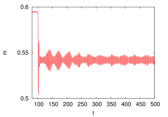
Figure 8: F-HMF model without an external field. Time evolution of the magnetization $m$: Starting with thermal equilibrium (3) at temperature $T=2$ and coupling constant $J=5$, the coupling is instantaneously quenched at $t=100$ to $J=4$. The number of particles is $N=10^{6}$.

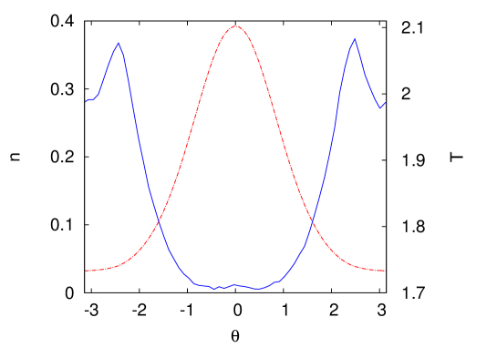
Figure 9: Temperature inversion in the F-HMF model after a quench of the coupling. Local density $n$ (red dot-dashed line) and local temperature $T$ (blue solid line) measured at $t=10^{3}$ in the QSS obtained under the same conditions as for Fig. 8.

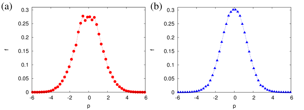
Figure 10: Momentum distribution of the F-HMF model measured at $t=10^{3}$ in the QSS obtained under the same conditions as for Fig. 8. (a) The distribution at $\vartheta=\pi$ at which the density is minimum. (b) The distribution at $\vartheta=0$ at which the density is maximum.

The physical picture based on wave-particle interactions and velocity filtration holds also in this case. We performed other numerical experiments with larger $N$’s and different values of $J$ and, as before, we can conclude that no fine tuning is needed to produce temperature inversion by means of a quench protocol, acting on either $h$ or on $J$.

Let us now discuss how the F-HMF model is related to a system of atoms interacting with a standing electromagnetic wave in an optical cavity, and how a quench of the coupling constant could be performed in a controlled way in a laboratory experiment.

3 Temperature inversion in a system of atoms in an optical cavity

Atoms interacting with a single-mode standing electromagnetic wave due to light trapped in a high-finesse optical cavity are subject to an interparticle interaction that is long-ranged owing to multiple coherent scattering of photons by the atoms into the wave mode [25, 26, 27]. The system serves as a unique platform to study long-range interactions, and in particular mean-field interactions, under tunable experimental conditions. The typical setup is sketched in Fig. 11, which also shows optical pumping by a transverse laser of intensity $\Omega^{2}$ to counter the inevitable cavity losses quantified by the cavity linewidth $\kappa$ (the lifetime of a photon in the cavity being $\kappa^{-1}$). We follow Ref. [25, 26, 27], and refer the reader to these works and to references therein for all the technical details that we skip here. Let us then consider a system of $N$ identical atoms of mass $m$. As far as the interactions with the electromagnetic field is concerned, each atom may be regarded as a two-level system, where the transition frequency between the two levels is $\omega_{0}$. If the atoms are confined in one dimension along the cavity axis (taken to be the $x$-axis), and $k$ is the wavenumber of the standing wave, the sum of the electric field amplitudes coherently scattered by the atoms at time $t$ depends on their instantaneous positions $x_{1},\ldots,x_{N}$, and is proportional to the quantity

$$\Theta\equiv\frac{1}{N}\sum_{j=1}^{N}\cos(kx_{j})\,,$$ (8)

so that the cavity electric field at time $t$ is $E(t)\propto\Theta\sqrt{N\overline{n}}$ [25]. Here, $\overline{n}$ is the maximum intracavity-photon number per atom, given by $\overline{n}\equiv N\Omega^{2}\alpha^{2}/(\kappa^{2}+\Delta_{c}^{2})$, with $\alpha\equiv g/\Delta_{a}$ being the ratio between the cavity vacuum Rabi frequency and the detuning $\Delta_{a}\equiv\omega_{L}-\omega_{0}$ between the laser and the atomic transition frequency, and $\Delta_{c}\equiv\omega_{L}-\omega_{c}$ being the detuning between the laser and the cavity-mode frequency. It is important to note that $\overline{n}$ is tunable by controlling either the strength of the external laser pump or the detuning $\Delta_{c}$. The quantity $\Theta$ characterizes the amount of spatial ordering of atoms within the cavity mode, with $\Theta=0$ corresponding to atoms being uniformly distributed and the resulting vanishing of the cavity field, and $|\Theta|\neq 0$ implying spatial ordering. In particular, $|\Theta|=1$ corresponds to perfect ordering of atoms to form Bragg gratings and the resulting scattering of photons in phase, thereby maximizing the cavity field, which in turn traps the atoms by means of mechanical forces. Note that the wave number $k$ is related to the linear dimension $L$ of the cavity through $k=2\pi/\lambda$ and $L=q\lambda$, where $\lambda$ is the wavelength of the standing wave, and $q\in\mathbb{N}$.

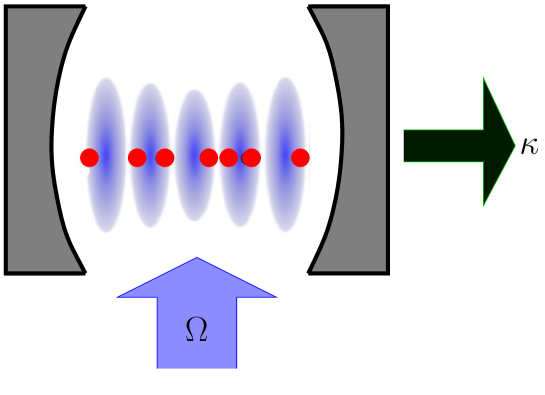
Figure 11: Atoms interacting with a single-mode standing electromagnetic wave in a cavity of linewidth $\kappa$, and being driven by a transverse laser with intensity $\Omega^{2}$.

The dynamics of the system may be conveniently studied by analyzing the time evolution of the $N$-atom phase space distribution $f_{N}(x_{1},\ldots,x_{N},p_{1},\ldots,p_{N},t)$ at time $t$, with $p_{j}$’s denoting the momenta conjugate to the positions $x_{j}$. Treating the cavity field quantum mechanically, and regarding the atoms as classically polarizable particles with semiclassical center-of-mass dynamics, it was shown that the distribution $f_{N}$ evolves in time according to the Fokker-Planck equation (FPE) [25, 26]

$$\partial_{t}f_{N}+\{f_{N},H\}=-\overline{n}\Gamma\mathcal{L}f_{N}\,.$$ (9)

Here, the operator $\mathcal{L}$ describes the dissipative processes (damping and diffusion) that explicitly depend on the positions and momenta of the atoms, and $\Gamma\equiv 8\omega_{r}\kappa\Delta_{c}/(\Delta_{c}^{2}+\kappa^{2})$, where $\omega_{r}\equiv\hbar k^{2}/(2m)$ is the recoil frequency due to collision between an atom and a photon, and $\hbar$ is the reduced Planck constant. The Hamiltonian $H$ is given by [25, 26]

$$H=\sum_{j=1}^{N}\frac{p_{j}^{2}}{2m}+N\hbar\Delta_{c}\overline{n}\,\Theta^{2}\,.$$ (10)

This semiclassical limit is valid under the condition of $\kappa$ being larger than $\omega_{r}$, and the Hamiltonian $H$ describes the conservative dynamical evolution of $f_{N}$ in the limit of vanishing cavity losses, or for times sufficiently small such that dissipative effects are negligible. The Hamiltonian (10) contains the photon-mediated long-ranged (mean-field) interaction between the atoms encoded in the quantity $\Theta$. Note that the interaction is attractive (respectively, repulsive) when $\Delta_{c}$ is negative (respectively, positive). On time scales sufficiently long so that the effect of the right-hand-side of Eq. (9) is non-negligible, the mean-field description of the dynamics is no longer valid [25, 27].

3.1 The dissipationless limit and the connection with the HMF model

Let us now consider the case of effective attractive interactions between the atoms and the cavity field ($\Delta_{c}<0$), and study the dynamics of the system in the limit in which the effect of the dissipation can be neglected, that is, for sufficiently small times. In this limit, the dynamics of the $N$ atoms is conservative and governed by the Hamiltonian $H$ given by Eq. (10). The positions $x_{j}$ of the atoms enter the Hamiltonian only as $kx_{j}$, so that we may define the phase variables

$$\vartheta_{j}=kx_{j}=2\pi\frac{x_{j}}{\lambda}~{},$$ (11)

for $j=1,\ldots,N$. Now, the length $L$ of the cavity is $q$ times the wavelength $\lambda$, with $q$ an integer. Then, setting the origin of the $x$-axis in the center of the cavity, we have $x_{j}\in[-q\lambda/2,q\lambda/2]$, so that on using the periodicity of the cosine function, we can take the phase variables $\vartheta_{j}$ modulo $q$ such that $\vartheta_{j}\in[-\pi,\pi]$. Then, by measuring lengths in units of the reciprocal wavenumber $k^{-1}=\lambda/(2\pi)$ of the cavity standing wave, masses in units of the mass of the atoms $m$, and energies in units of $\hbar\Delta_{c}$, the Hamiltonian can be rewritten in dimensionless form as

$$\mathcal{H}=\sum_{j=1}^{N}\frac{(p_{\vartheta})_{j}^{2}}{2}-\overline{n}N\Theta^{2}\,,$$ (12)

where, in terms of the $\vartheta$ variables, $\Theta$ is now expressed as

$$\Theta=\frac{1}{N}\sum_{j=1}^{N}\cos\vartheta_{j}\,.$$ (13)

The $(p_{\vartheta})_{j}$’s in Eq. (12) are the momenta canonically conjugated to the $\vartheta_{j}$ variables.

The similarity between the system with Hamiltonian (12) and an F-HMF model, already noted in [25], is now well apparent, since the expression of the interaction field $\Theta$ given in Eq. (13) coincides with the expression of the $x$-component of the magnetization of the HMF model. Indeed, the equations of motion derived from the Hamiltonian (12) read

$$\left\{\begin{array}[]{ccl}{\displaystyle\frac{{\rm d}\vartheta_{j}}{{\rm d}t}}&=&(p_{\vartheta})_{j}\,,\\ &&\\ {\displaystyle\frac{{\rm d}(p_{\vartheta})_{j}}{{\rm d}t}}&=&-\overline{n}\,\Theta\sin\vartheta_{j}\,,\end{array}\right.$$ (14)

for $j=1,\ldots,N$. Equations (14) coincide with Eqs.  (2) once $h=0$, $\Theta=m_{x}$, $m_{y}=0$ and $J=\overline{n}$. Hence, the dynamics of a system of atoms interacting with light in a cavity in the dissipationless limit is equivalent to that of a model that differs from the ferromagnetic HMF model in zero field just for the fact that particles in the former interact only with the $x$-component of the magnetization. Equivalently, the dynamics is equivalent to that of an HMF model with $m_{y}\equiv 0$. This means that the thermal equilibrium distribution for atoms in a cavity (still assuming that dissipative effects can be neglected) is still given by Eq. (3), with $h=0$ and $m_{y}=0$.

3.1.1 Quenching the coupling constant

In an HMF model in the thermodynamic limit $N\to\infty$, the condition $m_{y}\equiv 0$ holds for all times if it holds at $t=0$, that is, if the initial spatial distribution is symmetric around $\vartheta=0$. In a finite system, even starting from a symmetric distribution, $m_{y}$ will not stay exactly zero for all times, due to fluctuations induced by finite-size effects, but will remain very small. Hence, the numerical experiment reported in Sec. 2.2.2, which was performed while starting from an equilibrium state with $m_{y}(t=0)=0$, almost directly applies also to the model of atoms in an optical cavity (with $J=\overline{n}$), but for the fact that there was a coupling of the particles to the small fluctuating $y$-component of the magnetization in the former that would be absent in the atom case. It is reasonable to expect that this coupling has only a small effect, since $N$ is very large ($N=10^{6}$). To check this, we repeated the numerical experiment using the dynamics given by Eqs. (14), that is, we prepared the system in the same initial condition at $T=2$ and $\overline{n}=5$, then evolved the dynamics—now using Eqs. (14)—until $t=100$ when we quenched the coupling to the new value $\overline{n}=4$. The results are shown in Figs. 12, 13 and 14, that are essentially indistinguishable from Figs. 8, 9 and 10 of Sec. 2.2.2. There is clear temperature inversion, the momentum distribution exhibits the same features as before, and the average temperature has the value $\langle T\rangle\approx 1.76$ in the QSS, lower than the initial value of $2$.

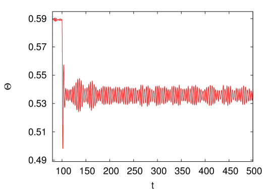
Figure 12: Atoms in a cavity in the dissipationless limit. Time evolution of the mean field $\Theta$: Starting with thermal equilibrium (3) at temperature $T=2$ and coupling constant $\overline{n}=5$, the coupling is instantaneously quenched at $t=100$ to $\overline{n}=4$. The number of particles is $N=10^{6}$.

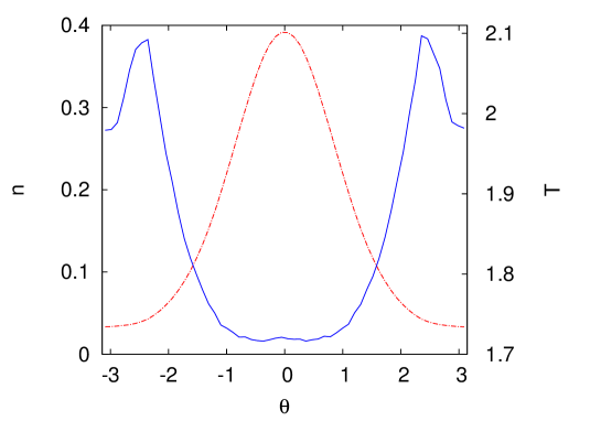
Figure 13: Temperature inversion in a system of atoms in a cavity after a quench of the coupling. Local density $n$ (red dot-dashed line) and local temperature $T$ (blue solid line) measured at $t=10^{3}$ in the QSS obtained under the same conditions as for Fig. 12.

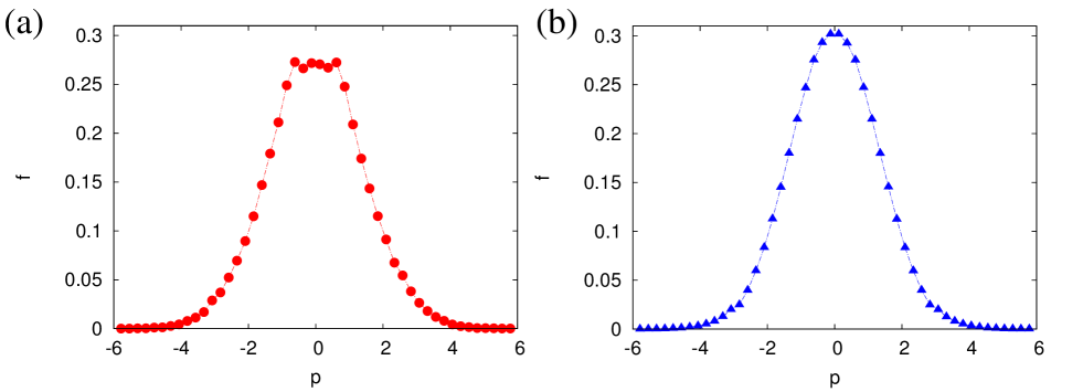
Figure 14: Momentum distribution of a system of atoms in a cavity measured at $t=10^{3}$ in the QSS obtained under the same conditions as for Fig. 12. (a) The distribution at $\vartheta=\pi$ at which the density is minimum. (b) The distribution at $\vartheta=0$ at which the density is maximum.

3.1.2 From numerical to laboratory experiments?

What do the results we have shown suggest as regards the possibility of observing temperature inversion in a laboratory experiment with atoms interacting with light in an optical cavity? To answer this question, let us consider the system and the values of the parameters that were already considered in Ref. [25] so that the semiclassical approximation for the atomic dynamics holds. We thus consider a system of ${}^{85}{\rm Rb}$ atoms, whose mass is $m\approx 1.4\times 10^{-25}$ kg; the atomic transition is the $D_{2}$ line, with a wavelength $\lambda_{0}=780$ nm. In terms of $\gamma=2\pi\times 3$ MHz, the half-width of the $D_{2}$ line, the cavity linewidth is $\kappa=0.5\gamma$ and the detuning is $\Delta_{c}=-\kappa$. The energy unit is thus $\hbar\Delta_{c}\approx 10^{-27}$ J. Preparing a system of atoms in a thermal state with a temperature of order unity in these energy units means reaching temperatures of the order of $10^{-4}$ K, which can be achieved with laser cooling techniques. Hence, the initial state we have considered in our simulations can be prepared in a laboratory, and, as already noted, $\overline{n}$ can be tuned in the range we considered (and even in a much wider range, if needed) so that also the quench of $\overline{n}$ is feasible. The crucial point is to understand whether the dissipationless limit corresponding to assuming a Hamiltonian dynamics reasonably describes the dynamics of the atoms over the timescale needed for the relaxation of the system to the QSS with temperature inversion. With our choice of energy, length and mass units, the time unit is fixed to

$$\tau=\sqrt{\frac{m\lambda_{0}^{2}}{4\pi^{2}\hbar\Delta_{c}}}\approx 10^{-6}~{}{\rm s},$$ (15)

this has to be compared with the timescale that rules the dissipative effects, $\tau_{c}=\kappa^{-1}\approx 10^{-7}$ s. Luckily enough, the simulations reported in Refs. [25, 26] show that the dissipative effects set in on a timescale that is of the order of $(10^{4}\div 10^{6})\tau_{c}$, while our simulations show that the QSS with temperature inversion is reached after times of the order of $(10^{2}\div 10^{3})\tau_{c}$, so that there should be ample room for measurements of temperature inversion before it is destroyed by dissipation.

4 Iterative cooling via temperature inversion

We have already noted in all the cases considered above that the system (be it an HMF or an atomic system) is colder in the QSS with temperature inversion than it was in the initial thermal equilibrium state. Moreover, the fact that the QSS has temperature inversion means that hotter particles reside in the external parts of the system, where the density is smaller. This suggests that temperature inversion could be exploited to make the system even colder by means of an iterative protocol that goes as follows. We prepare the system in an inhomogeneous thermal state at temperature $T$ symmetric about $\vartheta=0$, perform a quench, and let the system relax to the QSS with temperature inversion as before. Now, we filter out hotter particles, that is, all the particles that are located at $|\vartheta|>\vartheta_{c}$, with a suitable choice of $\vartheta_{c}$: the resulting system will be close to isothermal at a temperature $T^{\prime}<T$. We let the system relax for some time and then perform another quench. The system goes into another QSS with temperature inversion and average temperature $T^{\prime\prime}<T^{\prime}$. The protocol can be iterated as long as it continues to appreciably cool the system, or as long as there is room for another quench of the parameters.

We now show the results obtained by applying this iterative cooling protocol to the cases studied before.

4.1 Cooling the antiferromagnetic HMF model

We start with the AF-HMF model. After performing the quench described in Sec. 2.1.1, whereby starting in equilibrium at $J=-1$, $T=5$ and $h=15$, the field was quenched to $h=10$, the system is in a QSS with temperature and density profiles shown in Fig. 3. Now, we filter out the hotter (high-energy) particles, which we choose to be those with $\vartheta$’s lying outside the interval $[-2,2]$. Subsequently, we instantaneously quench the field from $h=10$ to $h=5$; the system eventually settles into a QSS, and the corresponding local density and local temperature profiles are shown in Fig. 15 (a). By further filtering out the high-energy particles and quenching instantaneously the field to $h=1.0$, the system goes to another QSS whose density and temperature profiles are reported in Fig. 15 (b). The average temperature as a function of time for the full sequence of events starting with equilibrium at $T=5$ and $h=15$ is shown in Fig. 16. The system cools down from an initial average temperature $\langle T\rangle=5$ to a final value $\langle T\rangle\approx 2$. Each small downward step in $\langle T\rangle(t)$ corresponds to filtering out the high-energy particles, while each large downward step corresponds to settling of the system into a QSS with a lower temperature as a result of quenching of the field to a lower value. The percentage decrease in the number of particles during filtering out the high-energy particles equals about $2.11\%$ during the first stage of filtration, and about $4.95\%$ during the second stage. Not surprisingly, the cooling protocol becomes less efficient at subsequent stages.

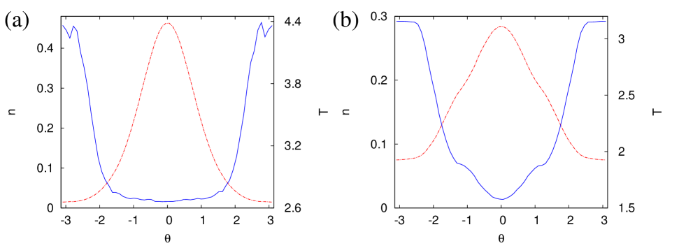
Figure 15: Iterative cooling in the AF-HMF model in presence of an external field. (a) Local density $n$ (red dashed-dotted line) and local temperature $T$ (blue solid line) in the QSS after the first filtering stage of the hot particles. (b) Local density $n$ (red dashed-dotted line) and local temperature $T$ (blue solid line) in the QSS after the second filtering stage. $N$ and $J$ values are the same as in Fig. 3.

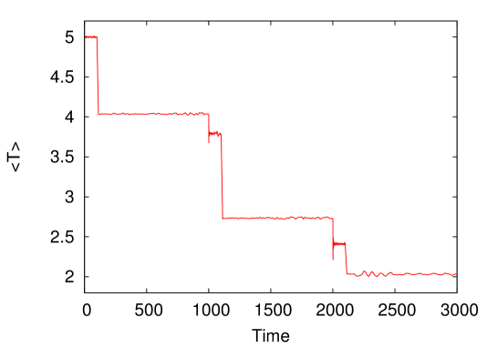
Figure 16: Iterative cooling in the AF-HMF model in presence of an external field. Average temperature $\langle T\rangle$ as a function of time for the full cooling protocol. $N$ and $J$ values are the same as in Fig. 3.

4.2 Cooling the ferromagnetic HMF model and atoms in a cavity

We now apply the same cooling protocol described above to the F-HMF model in an external field, while starting from equilibrium at $J=1$, $T=5$ and $h=15$. The results are shown in Figs. 17 and 18. Again, we obtain a cooling from an initial average temperature $\langle T\rangle=5$ to a final value $\langle T\rangle\approx 2$. The percentage decrease in the number of particles during filtering out the high-energy particles equals about $1.24\%$ during the first stage of filtration, and equals about $3.16\%$ during the second stage.

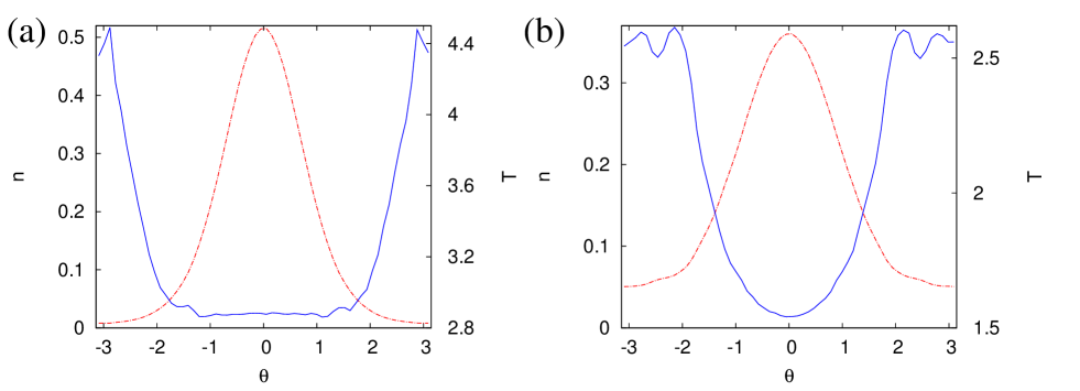
Figure 17: Iterative cooling in the F-HMF model in presence of an external field. (a) Local density $n$ (red dashed-dotted line) and local temperature $T$ (blue solid line) in the QSS after the first filtering stage of the hot particles. (b) Local density $n$ (red dashed-dotted line) and local temperature $T$ (blue solid line) in the QSS after the second filtering stage. $N$ and $J$ values are the same as in Fig. 6.

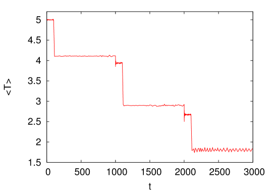
Figure 18: Iterative cooling in the F-HMF model in presence of an external field. Average temperature $\langle T\rangle$ as a function of time for the full cooling protocol. $N$ and $J$ values are the same as in Fig. 6.

We now turn to the case of a quench of the coupling constant, still for the F-HMF model but now without external field. The cooling protocol goes as before, but we can fruitfully perform only one stage of filtering instead of two. We start with the equilibrium state at $T=2$ and $J=5$ that is quenched to $J=4$, yielding the QSS whose density and temperature profiles are shown in Fig. 9. We then filter out the hotter particles, in this case defined as those with $\vartheta$’s lying outside the interval $[-1,1]$. Subsequently, we instantaneously quench the coupling to $J=3$. The density and temperature profile in the resulting QSS are shown in Fig. 19, and the time evolution of the average temperature is reported in Fig. 20. Under the full quenching protocol, the system cools down from an initial average temperature $\langle T\rangle=2$ to a final value $\langle T\rangle\approx 1.0$. The percentage decrease in the number of particles during filtering out the high-energy particles equals about $34.3\%$.

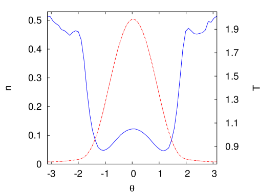
Figure 19: Iterative cooling in the F-HMF model without external field: local density $n$ (red dashed-dotted line) and local temperature $T$ (blue solid line) in the QSS after the filtering stage of the hot particles. $N$ value is the same as in Fig. 9.

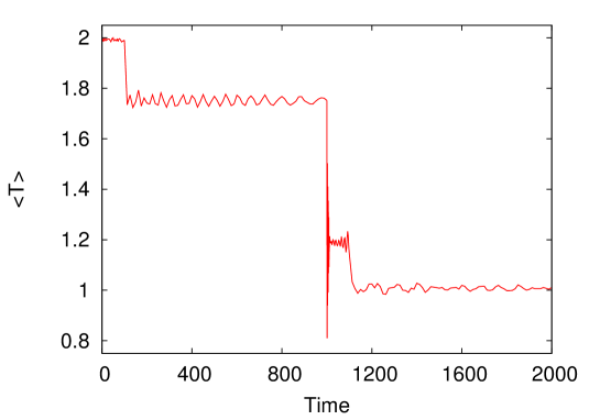
Figure 20: Iterative cooling in the F-HMF model without an external field. Average temperature $\langle T\rangle$ as a function of time for the full cooling protocol. $N$ value is the same as in Fig. 9.

Finally, we apply exactly the same cooling protocol to the dynamics of atoms in a cavity, given by Eqs. 14. The results are shown in Figs. 21 and 22, and as expected are very close to that obtained for the F-HMF model: the system under the quenching protocol cools down, from an initial average temperature $\langle T\rangle=2$ to a final value $\langle T\rangle\approx 1$. The percentage decrease in the number of particles during filtering out the high-energy particles equals about $34.5\%$.

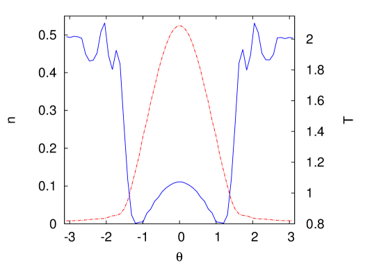
Figure 21: Iterative cooling of atoms in a cavity: local density $n$ (red dashed-dotted line) and local temperature $T$ (blue solid line) in the QSS after the filtering stage of the hot particles. The value of $N$ is the same as in Fig. 13.

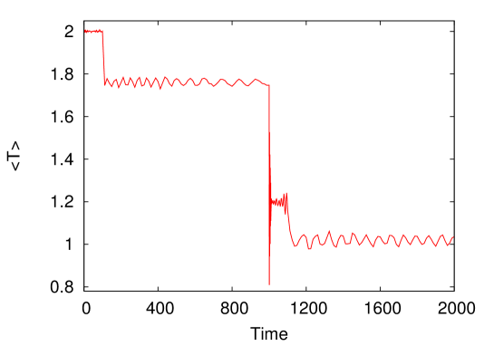
Figure 22: Iterative cooling of atoms in a cavity: average temperature $\langle T\rangle$ as a function of time for the full cooling protocol. $N$ value is the same as in Fig. 13.

Although the cooling protocol does not yield dramatic results, especially in the last two considered cases, still it seems able to (at least) decrease the temperature of a system by a factor of two. Moreover, it opens up the possibility of a different way of cooling a system with respect to the nowadays commonly used ones.

5 Concluding remarks

In this paper, we have demonstrated that quasi-stationary states that an isolated long-range interacting system relaxes to when starting from a spatially inhomogeneous thermal equilibrium and subsequently subject to a quench of one of the parameters of the Hamiltonian generically exhibit the phenomenon of temperature inversion. Using molecular dynamics simulations of a prototypical model, the HMF model, we have shown that different quench protocols lead to temperature inversion, in presence and in absence of an external field, and with both attractive and repulsive interactions: no fine-tuning is necessary in any of the cases. This lends further support to the claim made in [11, 15] that, rather than a peculiarity of some astrophysical systems, temperature inversion should be a “universal” feature of nonequilibrium quasi-stationary states resulting from perturbations of spatially inhomogeneous thermal equilibrium. Moreover, our analysis of the momentum distribution functions supports the interpretation put forward in [11] that temperature inversion arises due to an interplay between wave-particle interaction (the role of the wave being played by the oscillation of the mean field induced by the perturbation or the quench) and velocity filtration. The latter is a mechanism proposed by Scudder [21, 22, 23] to explain the temperature profile of the solar corona, and basically amounts to the statement that a suprathermal velocity distribution becomes broader when climbing a potential well.

The fact that quench protocols are able to produce temperature inversions is of particular relevance in view of observing this phenomenon in controlled laboratory experiments. Exploiting the close connection between the HMF model and a model describing the dynamics of a system of atoms interacting with light in an optical cavity, as noted in Ref. [25], we have argued that a quench of the external laser pump should be able to produce a quasi-stationary state with temperature inversion in a system of, say, Rubidium atoms in a cavity that is initially in thermal equilibrium at temperatures reachable by laser cooling. Such a quasi-stationary state should survive for quite a long time before being destroyed by dissipative effects. The latter claim is made on the assumption that the timescales of dissipation are the same as those observed in [25, 26]. Similar to our study, these works also considered a quench of the coupling constant, but from different initial states and to different final states, and this may affect the dissipation timescales. However, results in [26] seem to indicate that dissipation is inhibited in spatially inhomogeneous states, and this would be an advantage for a quench experiment like those suggested here. An interesting follow-up of the present work, in view of a detailed study of the feasibility of an experiment, would surely be to use the techniques of [25, 26] to study the evolution after quenches like the ones described here under a dynamics that fully takes into account the dissipative effects. Another interesting system to study in view of a possible experiment to detect temperature inversion would be a system of trapped ions, which may be related to the antiferromagnetic HMF model. Work is in progress along this direction [33].

Finally, we have shown that temperature inversion may be exploited to cool the system. The cooling protocol is of iterative type, and takes advantage of the fact that in states with temperature inversion hotter particles are spatially separated from colder ones, so that they can be filtered out. Let us sign off by saying that temperature inversion is one of many fascinating features of the nonequilibrium states of long-range interacting systems that are yet to be unveiled.

6 Acknowledgments

We thank P. Di Cintio, H. Landa and A. Trombettoni for fruitful discussions and suggestions. SG acknowledges the support and hospitality of INFN (Italy) and the University of Florence.

References

- [1] Campa A, Dauxois T and Ruffo S 2009 Statistical mechanics and dynamics of solvable models with long-range interactions Phys. Rep. 480 57
- [2] Bouchet F, Gupta S and Mukamel D 2010 Thermodynamics and dynamics of systems with long-range interactions Physica A: Special Issue FPSP XII 389 4389
- [3] Campa A, Dauxois T, Fanelli D and Ruffo S 2014 Physics of Long-Range Interacting Systems (Oxford: Oxford University Press)
- [4] Choudouri A R 2010 Astrophysics for Physicists (Cambridge: Cambridge University Press)
- [5] Binney J and Tremaine S 2008 Galactic Dynamics, 2nd ed. (Princeton: Princeton University Press)
- [6] Lynden-Bell D 1967 Statistical mechanics of violent relaxation in stellar systems Mon. Not. R. Astron. Soc. 136 101
- [7] Levin Y, Pakter R, Rizzato F B, Teles T N and Benetti F P C 2014 Nonequilibrium statistical mechanics of systems with long-range interactions Phys. Rep. 535 1
- [8] Benetti F P C, Ribeiro-Teixeira A C, Pakter R and Levin Y 2014 Nonequilibrium Stationary States of 3D Self-Gravitating Systems Phys. Rev. Lett. 113 100602
- [9] Leoncini X, Van Der Berg T N and Fanelli D 2009 Out-of-equilibrium solutions in the XY-Hamiltonian Mean-Field model Europhys. Lett. 86 20002
- [10] De Buyl P, Mukamel D and Ruffo S 2011 Self-consistent inhomogeneous steady states in Hamiltonian mean-field dynamics Phys. Rev. E 84 061151
- [11] Teles T N, Gupta S, Di Cintio P and Casetti L 2015 Temperature inversion in long-range interacting systems Phys. Rev. E 92 020101(R)
- [12] Teles T N, Gupta S, Di Cintio P and Casetti L 2016 Reply to ‘Comment on “Temperature inversion in long-range interacting systems”’ Phys. Rev. E 93 066102
- [13] Golub L and Pasachoff J M 2009 The Solar Corona (Cambridge: Cambridge University Press)
- [14] Myers P C and Fuller G A 1992 Density structure and star formation in dense cores with thermal and nonthermal motions Astrophys. J. 396 631
- [15] Casetti L and Gupta S 2014 Velocity filtration and temperature inversion in a system with long-range interactions Eur. Phys. J. B 87 91
- [16] Antoni M and Ruffo S 1995 Clustering and relaxation in Hamiltonian long-range dynamics Phys. Rev. E 52 2361
- [17] Di Cintio P, Gupta S and Casetti L 2016 Dissipationless collapse and the origin of temperature inversion in galactic filaments in preparation
- [18] Teles T N, Levin Y, Pakter R and Rizzato F P 2010 Statistical mechanics of unbound two-dimensional self-gravitating systems J. Stat. Mech.: Theory Exp. P05007
- [19] Worrakitpoonpon T 2011 Relaxation of isolated self-gravitating systems in one and three dimensions PhD Thesis
- [20] Campa A, Gupta S and Ruffo S 2015 Nonequilibrium inhomogeneous steady state distribution in disordered, mean-field rotator systems J. Stat. Mech.: Theory Exp. P05011
- [21] Scudder J 1992 On the causes of temperature change in inhomogeneous low-density astrophysical plasmas Astrophys. J. 398 299
- [22] Scudder J 1992 Why all stars should possess circumstellar temperature inversions Astrophys. J. 398 319
- [23] Scudder J 1994 Ion and electron suprathermal tail strengths in the transition region: Support for the velocity filtration model of the corona Astrophys. J. 427 446
- [24] A primer on velocity filtration is given in the Supplementary material to [11] at http://link.aps.org/supplemental/10.1103/PhysRevE.92.020101
- [25] Schütz S and Morigi G 2014 Prethermalization of atoms due to photon-mediated long-range interactions Phys. Rev. Lett. 113 203002
- [26] Schütz S, Jäger S B and Morigi G 2015 Relaxation after quenches in systems with photon-mediated long-range interactions arXiv:1512.05243
- [27] Jäger S B, Schütz S and Morigi G 2016 Mean-field theory of atomic self-organization in optical cavities arXiv:1603.05148
- [28] McLachlan R I and Atela P 1992 The accuracy of symplectic integrators Nonlinearity 5 541
- [29] Choudhouri A R 1998 The Physics of Fluids and Plasmas (Cambridge: Cambridge University Press)
- [30] Mohout C and Villani C 2011 On Landau damping Acta Mathematica 207 29
- [31] Barré J, Olivetti A and Yamaguchi Y Y 2010 Dynamics of perturbations around inhomogeneous backgrounds in the HMF model J. Stat. Mech.: Theory Exp. P08002
- [32] Barré J, Olivetti A and Yamaguchi Y Y 2011 Algebraic damping in the one-dimensional Vlasov equation J. Phys. A: Math. Theor. 44 405502
- [33] Landa H, Gupta S, Di Cintio P and Casetti L 2016 in preparation