Stabilizing Linear Prediction Models using Autoencoder

Abstract

To date, the instability of prognostic predictors in a sparse high dimensional model, which hinders their clinical adoption, has received little attention. Stable prediction is often overlooked in favour of performance. Yet, stability prevails as key when adopting models in critical areas as healthcare. Our study proposes a stabilization scheme by detecting higher order feature correlations. Using a linear model as basis for prediction, we achieve feature stability by regularizing latent correlation in features. Latent higher order correlation among features is modelled using an autoencoder network. Stability is enhanced by combining a recent technique that uses a feature graph, and augmenting external unlabelled data for training the autoencoder network. Our experiments are conducted on a heart failure cohort from an Australian hospital. Stability was measured using Consistency index for feature subsets and signal-to-noise ratio for model parameters. Our methods demonstrated significant improvement in feature stability and model estimation stability when compared to baselines.

1 Introduction

Healthcare data is expected to increase by fifty-fold in the coming years [16]. While the direction of current machine learning research is to handle such data, clinical interpretability of models is often overlooked. In healthcare, interpretability is the ability of the model to explain the reason behind prognosis. Such models identify a small subset of strong features (predictors) from available data, and rank them according to their predictive power [28]. This act of feature selection and ranking need to be stable in the face of data re-sampling to ensure clinical adoption. Nonetheless, the nature of clinical data introduces several challenges.

For a particular condition, training data derived from electronic medical records (EMR) usually consist of small number of cases with a large number of events. Most of these events have high correlation with each other. As example, emergency admission events will be correlated with ward transfers, diagnosis of co-occurring diseases (heart failure and diabetes) will have high correlation, pathological measurements (amount of Sodium and Potassium in the body) will be related. To avoid over-fitting, such data require sparse methods in feature selection and learning [24]. But sparsity in correlated features causes instability and results in non-reproducible models [2, 12].

In the presence of correlated features, automatic feature selection using lasso has proven to be unstable for linear [27] and survival models [12]. Recent studies propose adapting lasso to acknowledge feature correlations. Such correlations or groupings can be identified using cluster analysis [1, 13, 15] or density estimation [25]. Group lasso and its variants have been introduced for scenarios where feature groupings are predefined [26, 7]. When the features are ordered, or at least have a specification of the nearest neighbour of each feature, Tibshirani et al. proposed fused lasso to perform feature grouping [21]. In contrast, elastic net regularization forces sharing of statistical weights in correlated features without imposing any preconditions on data [29]. When applied to clinical prediction, elastic net regularization proved superior to lasso for prostate cancer dataset [19]. Another approach to stabilize a sparse model is by additional regularization using graphs, where the nodes are features and edges represent relationships [18]. This strategy has been successfully applied in bioinformatics, where feature interactions have been extensively documented and stored in online databases [11, 5]. In clinical setting, recent studies have used covariance graph [9] and hand crafted feature graph using semantic relations in ICD-10 diagnosis codes and intervention codes [6] as solutions to the instability problem. However, these studies did not consider higher order correlations, and lacked capability to automatically learn feature groupings.

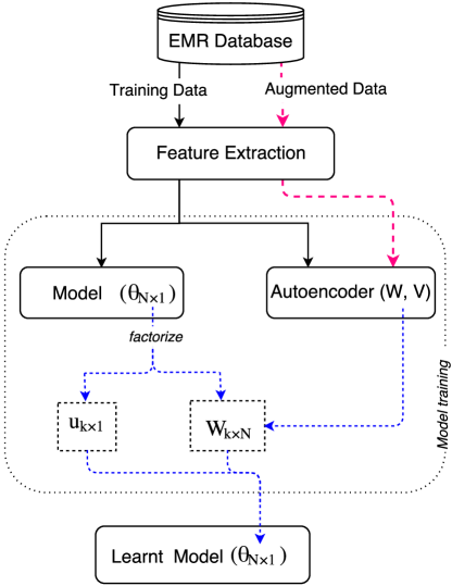
Figure 1: The work-flow diagram of our framework for deriving autoencoder stabilized prediction model from EMR. The model parameter $\theta$ is factorized into a lower dimensional vector $u$ and high dimensional matrix $W$. The $W$ matrix is jointly modelled as encoding weights in an autoencoder network and is used to regularize the prediction model.

In this paper, we propose a novel methodology to stabilize a sparse high dimensional linear model using recent advances in deep learning and self-taught learning [17]. We propose that the linear model parameter $\theta$ is a combination of a lower dimensional vector $u$, and a high dimensional matrix $W$, where $W$ encapsulates the feature correlations. By modelling $W$ as the encoding weights of an autoencoder network, we capture higher order feature correlations in data. The workflow diagram of our method is illustrated in Fig.1.

To minimize variance in feature subsets and parameter estimation, we introduce three regularizers for our sparse linear model: 1) autoencoder derived from training cohort, 2) combination of autoencoder and feature graph derived from training cohort, 3) combination of feature graph derived from training cohort and autoencoder derived from augmenting an external cohort to training data. This process of augmenting external data to autoencoder training results in more robust estimation of higher order correlation matrix $W$.

We conducted our experiments on $1,885$ heart failure admissions from an Australian hospital. The augmented external data consisted of $2,840$ diabetic admissions. Feature stability was measured using consistency index [10]. Parameter estimation stability was measured using signal-to-noise ration (SNR). Our proposed stabilization methods demonstrated significantly higher stability when compared with the baselines.Our contribution is in understanding the need for stable prediction, when much research has been dedicated to improving performance. For critical applications like healthcare, where data is sparse and redundant, stable features and estimates are necessary to lend credence to the model and its performance.

2 Framework

Sparse generalized linear models take the form $f(x)=\theta^{T}x$ subject to $\sum_{i=1}^{N}|\theta_{i}|\leq\alpha$, where $\theta\in\mathbb{R}^{N}$ is the model parameter derived from data: $\boldsymbol{x}\in\mathbb{R}^{N}$. Here, $\alpha$ is the sparsity controlling parameter, typically enforced using lasso regularization [20]. More formally, let $\mathcal{D}=\left\{\boldsymbol{x}_{m},\,y_{m}\right\}_{m=1}^{M}$ denote the training data, where $\boldsymbol{x}_{m}\in\mathcal{R}^{N}$ denotes the high dimensional feature vector of data instance $m$, and $y_{m}$ is the outcome (for example, the occurrence of future readmission). If $\mathcal{L}(\theta|\mathcal{D})$ is a linear loss, we have:

$$\mathcal{L}_{\text{lasso}}=\frac{1}{M}\mathcal{L}(\theta|\mathcal{D})+\alpha\sum_{i=1}^{N}|\theta_{i}|$$ (1)

where $\alpha>0$ controls the sparsity of the model parameters. The lasso regularization forces the weights of weak parameters towards zero. However, enforcing sparsity on high-dimensional, highly correlated and redundant data, as derived from EMR causes the following problems.

First, lasso regularization randomly chooses one feature from a correlated pair. The EMR data has a high degree of correlation and redundancy in hospital recorded events. Since lasso favours stronger predictors, each feature from a highly correlated pair will only have about 50% chance in being selected during every training run. Second, in clinical scenario, a large collection of features could be weakly predictive for a condition or medical event. Lasso could ignore such feature groups due to low selection probabilities [14].

This sparsity-stability predicament can be resolved by forcing correlated features to have similar weights. The traditional approach is to modify lasso regularization with elastic net [29] as:

$$\mathcal{L}_{\text{elastic net}}=\frac{1}{M}\mathcal{L}(\theta|\mathcal{D})+\alpha\left(\lambda_{\text{en}}\sum_{i}|\theta_{i}|+(1-\lambda_{\text{en}})\sum_{i}\theta_{i}^{2}\right)$$

Here, the ridge regression term $\sum_{i}\theta_{i}^{2}$ encourages correlated feature pairs to have similar weights, and $\lambda_{\text{en}}\in[0,1]$ balances the contribution of lasso term $\sum_{i}|\theta_{i}|$ and ridge regression term $\sum_{i}\theta_{i}^{2}$. However, elastic net forces the weights to be equally small, resulting in lesser sparsity.

Another recent work introduces a feature graph built from hierarchical relations in ICD-10 diagnosis codes and intervention codes [6]. A Laplacian of this feature graph: $\mathbf{L}$, is used to ensure weight sharing between related features as:

$$\mathcal{L}_{\text{feature graph}}=\mathcal{L}_{\text{lasso}}+\frac{1}{2}\,\lambda_{\text{fg}}(\theta^{T}\mathbf{L}\theta)$$ (2)

We propose to automatically learn higher order correlations in data.

2.1 Correlation by Factorization in Linear Models

To model higher order correlations in data, we begin by decomposing model parameter $\theta$ into a lower order vector and a high dimensional matrix as: $\theta_{\text{N}\times 1}=W_{k\times\text{N}}^{T}\,u_{k\times 1}$, where $k\ll\text{N}$. This factorization offers several advantages. The lower dimensionality of $u$ makes it more easier to learn and more stable to data variations. The $W$ captures higher order correlations that be modelled using different auxiliary tasks. Greater number of tasks ensure better solution, since there are more constraints.

As a concrete example for generalized linear models, we work on binary prediction using logistic regression. The modified logistic loss function $\mathcal{L}(\theta|\mathcal{D})$ using $u$ and $W$ becomes:

$$\mathcal{L}_{\text{logit}}(u,W\,|\mathcal{D}) = \text{log}(1+\text{exp}(-yu^{T}W\boldsymbol{x}))$$

$$= \text{log}(1+\text{exp}(-yu^{T}z))$$

where $y\in\pm 1$ represents the data label. Notice that $z=W\boldsymbol{x}$ is a data transformation from N dimensions to the smaller $k$ dimension. To learn $W$, we need to choose a competent auxiliary task. We model $W$ as the encoding weights of a classical autoencoder derived from the same data $\mathcal{D}$.

2.2 Learning Higher Order Correlations using Autoencoder

An autoencoder is a neural network that learns by minimizing the reconstruction error using back-propagation [3]. The learning process is unsupervised, wherein the model learns the useful properties of the data. An autoencoder network consists of two components: (1) An encoder function that maps the input data $\boldsymbol{x}\in\mathbb{R}^{N}$ as: $h(x)=\sigma(W\boldsymbol{x}+b_{W})$ , where $\sigma$ can be any non-linear function (for e.g., the sigmoid function) and $W,b_{W}$ are the weights and bias of the hidden layer (2) A decoder function that attempts to reconstruct the input data as: $\tilde{x}=Vh+b_{V}$, where $V,b_{V}$ are the weights and bias of the output layer. The loss function is modelled as the reconstruction error:

$$\mathcal{L_{\text{AE}}}(W,V,b_{W,}b_{V}|\mathcal{D})=\frac{1}{2N}||x-b_{V}-V\sigma(Wx+b_{W})||_{2}^{2}$$ (4)

Once trained, evaluating a feed forward mapping using the encoder function gives a latent representation of the data. When the number of hidden units is significantly lesser than the input layer, $W$ encapsulates the higher order correlations among features.

We propose to regularize our sparse linear model in (2.1) using the autoencoder framework in (4). The joint loss function becomes:

$$\mathcal{L}_{\text{model}}(u,W,V,b_{W},b_{V}|\mathcal{D}) = \mathcal{L}_{\text{logit}}(u,W\,|\mathcal{D})+$$

$$+ \alpha\underset{{}_{i}}{\varSigma}|\underset{{}_{k}}{\varSigma}W_{ik}^{T}u_{k}|$$

$$+ \lambda_{\text{AE}}\mathcal{\,L_{\text{AE}}}(W,V,b_{W},b_{V}|\mathcal{D})$$

$$+ \lambda_{\ell 2}\left(W^{2}+V^{2}+b_{W}^{2}+b_{V}^{2}\right)$$

where $\alpha>0$ is the lasso regularization parameter which ensures weak $\theta_{i}=\underset{{}_{k}}{\varSigma}W_{ik}^{T}u_{k}$ are driven to zero. While $\lambda_{\text{AE}}$ controls the amount of regularization due to higher order correlation, $\lambda_{\ell 2}$ controls overfitting in autoencoder. The loss function in (2.2) is non-convex. We propose two extensions to our model.

2.2.1 Augmenting Feature Graph regularization

While autoencoders can be used to find automatic feature grouping, we can also exploit the predefined associations in patient medical records. For example, diseases or conditions reoccurring over multiple time-horizons should be assigned similar importance [22]. Also, the ICD-10 diagnosis and procedure codes are hierarchical in nature [23, 6]. We build a feature graph using these associations (as in (2)) and use it to further regularize our model in (2.2) as:

$$\mathcal{L}_{\text{model-fg}}(u,W,V,b_{W},b_{V}|\mathcal{D}) = \mathcal{L}_{\text{model}}(u,W,V,b_{W},b_{V}|\mathcal{D})$$

$$+ \frac{1}{2}\,\lambda_{\text{fg}}\left[(u^{T}W)\mathbf{\,L}\,(W^{T}u)\right]$$

2.2.2 Augmenting External data for Autoencoder learning

The encoding weights $W$ in (4) can be estimated from multiple sources. For example, in this paper, we propose to augment the current training data $\mathcal{D}$ (for example: heart failure cohort) with another cohort containing the same features (say, diabetic cohort). Training the autoencoder network on this augmented data will result in more robust estimation of $W$.

3 Experiments

The feature stability and model stability of our proposed framework is evaluated on heart failure (HF) cohort from Barwon Health, a regional hospital in Australia serving more than 350,000 residents. The Autoencoder learning was augmented with diabetes (DB) cohort from the same hospital. We mined the hospital EMR database for retrospective data for a period of 5 years (Jan 2007 to Dec 2011), focusing on emergency and unplanned admissions of all age groups. Inpatient deaths were excluded. All patients with at least one ICD-10 diagnosis code I50 were included in the HF cohort. The DB cohort contained all patients with at least one diagnosis code between E10-E14. This resulted in $1,885$ heart failure admissions and $2,840$ diabetic admissions. Table 1 shows the details of both cohorts.

Table 1: Characteristics of heart failure and diabetes cohort.

	Heart Failure (HF)		Diabetes (DB)
	Derivation	Validation	(Augmented data)
Admissions	1,415	369	2,840
Unique patients	1,088	317	1,716
Gender:
Male	541 (49.7%)	155 (48.9%)	908 (52.9%)
Female	547 (50.2%)	162 (51.1%)	808 (47.1%)
Mean age (years)	78.3	79.4	57.1
Mean Length of Stay	5.2 days	4.5 days	4.1 days
Total Features	3,338		6,711
Common features	558

The different features in EMR database (diagnosis, medications, treatments, procedures, lab results) were extracted using a one-sided convolutional filter bank introduced in [22]. The feature extraction process resulted in $3,338$ features for HF and $6,711$ features for DB cohort. A total of $558$ features were common to both cohorts (Table. 1).

3.1 Models and Baselines

From this data, we derive a lasso regularized logistic regression model to predict heart failure readmissions in 6 months. We force lasso to consider higher order correlations in data by using the following three regularization schemes:

3.1.1 Lasso-Autoencoder

The linear model is regularized by an autoencoder derived from HF cohort.

3.1.2 Lasso-Autoencoder-Graph

We construct a feature graph from $3,338$ features in HF cohort as in [6], and use it to further regularize the Lasso-Autoencoder model.

3.1.3 AG-Lasso-Autoencoder-Graph

AG denotes augmented data used to train the autoencoder. To estimate W, we used DB cohort augmented to the HF cohort. Training data consisted of $558$ features common to both HF and DB. The sparse prediction model was built from common features in HF cohort, and regularized using a HF-based feature graph and autoencoder from augmented data.

We compare the stability of our proposed regularization methods with the following baselines: 1) pure lasso 2) elastic net and 3) recently introduced feature graph regularization (as in [6]) .

3.2 Temporal Validation

The training and testing data were separated in time and patients. Patients discharged before September 2010 were included in training set. The validation set consisted of new admissions from September 2010 to December 2011. Model performance was measured using AUC (area under the ROC curve) based on Mann-Whitney statistic. A pre-defined threshold was used (chosen to maximize the F-score) to predict readmissions.

3.3 Measuring Stability

Variability in data resampling was simulated using bootstraps. We trained all models using $500$ bootstraps of randomly sampled training data. At the end of each bootstrap, the features selected by a model were ranked based on importance. Feature importance was calculated as the product of mean feature weights across all bootstraps and feature standard deviation in the training data. The top $k$ ranked features were collected to form a list of feature subsets: $S=\{S_{1},\,S_{2},\,\cdots,\,S_{500}\}$, where $|S_{i}|=k$.

We used consistency index [10] to measure pairwise feature subset stability. For a pair of subsets $(S_{i},\,S_{j})$, with length $k$ selected from a total of $d$ features, consistency index becomes:

$$\text{CI}(S_{i},\,S_{j})=\frac{rd-k^{2}}{k(d-k)}$$

where $r=|S_{i}\cap S_{j}|$. The overall stability score is the average of pairwise consistency index among all pairs. This stability score is bounded in $[-1,\,+1]$, with $-1$ for no overlap, $0$ for independently drawn subsets, and $+1$ complete overlap of two subsets. The score calculation is monotonous and corrects overlap due to chance [10].

The stability of estimated model parameters was measured using signal-to-noise ratio (SNR). The variance in estimation of feature $i$ can be calculated as:

$$\text{SNR}(i)=\nicefrac{{w_{i}}}{{\sigma_{i}}}$$

where $w_{i}$ is the mean feature weight across bootstraps for feature $i$, and $\sigma_{i}$ is its standard deviation.

4 Results

In this section, we demonstrate the effect of autoencoder regularization on model performance and stability, and compare with our baselines. The prediction models for heart failure readmission were derived from $3,338$ features extracted from hospital database. The self taught learning stage during autoencoder training used an augmented $2,840$ diabetic admissions with $558$ features that were common in both cohorts. A grid search for the best hyper-parameter setting resulted in $\alpha=.001$, $\lambda_{\text{en}}=.01$, $\lambda_{\text{graph}}=.03$ for the baseline models, and $\alpha=.005$, $\lambda_{\text{AE}}=3000$, $\lambda_{\text{graph}}=0.3$ for our autoencoder regularized models.

4.1 Capturing Higher Order Correlations

The efficacy of autoencoder network to model higher order correlations was verified by comparing the correlation matrices of raw data and data from the encoding layer. The autoencoder derived correlation matrix was denser (matrix mean = $0.19$) than the correlation matrix for raw data (matrix mean = $0.05$).

4.2 Effect on Model Sparsity

Table  2 provides a summary of the effects of stabilization schemes on model sparsity. Autoencoder regularization resulted in sparser models with no loss in performance.

Table 2: Effect of stabilization methods on model sparsity

Regularization	Features Selected (%)
Lasso	550  (16.5 %)
Elastic Net	753  (22.6 %)
Lasso-Graph	699  (20.9 %)
Lasso-Autoencoder	513 (15.4 %)
Lasso-Autoencoder-Graph	503 (15.1 %)
AG-Lasso-Autoencoder-Graph	412 (12.3 %)

Model performance was measured using area under the ROC curve (AUC). For autoencoder regularization, AUC critically depended on the choice of autoencoder penalty ($\lambda_{\text{AE}}$) and number of hidden units (see Fig. 2).

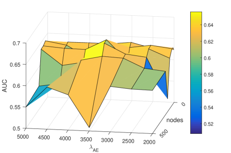
Figure 2: Effect of number of hidden units (nodes) and autoencoder penalty ($\lambda_{\text{AE}}$) on AUC. Lasso parameter fixed at $\alpha=.005$

A maximum AUC of 0.65 was obtained for AG-Lasso-Autoencoder-Graph model with 20 hidden units and hyperparameters as $\alpha=.005$, $\lambda_{\text{en}}=.03$, $\lambda_{\text{graph}}=.3$, $\lambda_{\text{AE}}=3000$.

4.3 Effect on Stability

When compared to $\lambda_{\text{AE}}$, the choice of hidden units had more influence on feature stability (see Fig. 3).

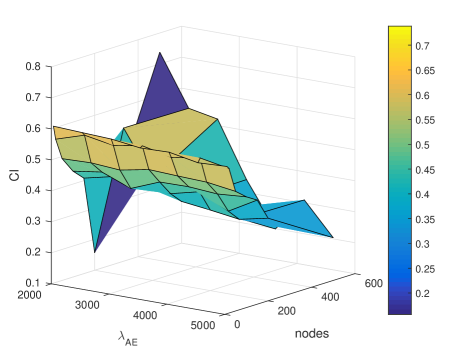
Figure 3: Effect of number of hidden units (nodes) and autoencoder penalty ($\lambda_{\text{AE}}$)feature stability measured by consistency of top 100 features. Lasso parameter fixed at $\alpha=.005$

Consistency index measurements for feature selection stability is reported in Fig. 4.

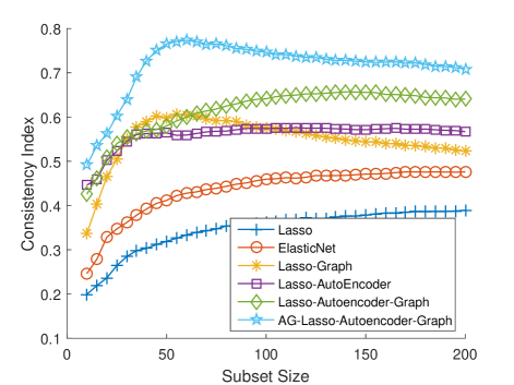
Figure 4: Feature stability as measured using Consistency Index. The plot compares similarity in feature subsets generated by our proposed models and baselines. Higher values indicate more stability.

In general, capturing higher order correlations using autoencoder improved feature stability when compared to baselines. Even though pure autoencoder regularization proved to be more effective for larger feature sets (> 120), the combination of autoencoder and graph regularization consistently outperformed the baselines. Further, augmenting external cohort to autoencoder learning resulted in the most stable features. Similar observations were made when measuring model estimation stability. Fig. 5 reports the signal-to-noise ratios of the top 50 individual features.

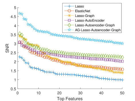
Figure 5: Model stability as measured using signal-to-noise ratio (SNR) of feature weights. Higher values indicate more stability.

At 95% CI (approximately 1.96 std), lasso regularization identifies 3 features, elastic net identifies: 21, Graph regularization: 24, while the autoencoder regularized models identify all the 50 features. The variance in feature weight is greatly reduced by AG-Lasso-Autoencoder-Graph regularization.

5 Discussion and Conclusion

Sparsity and stability are two important characteristics of interpretable healthcare. Sparsity promotes interpretability and stability inspires confidence in the prediction model. Through our experiments, we have demonstrated that autoencoder regularization, when applied to high-dimensional clinical prediction results in a sparse model that is stable in features and estimation. Our proposed model is built from common clinical and administrative data recorded in the hospital database, and hence can be easily integrated into existing systems.

The predictive performance of our proposed model (as measured by AUC) is comparable with existing studies [4]. Our stabilization scheme did not improve classification performance. A similar observation was made by Kalousis et al. in their study on high dimensional feature selection stability [8]. However, as their study noted, stable models impart confidence on the features selected, and in turn lends credence to corresponding classification performance.

5.1 Conclusion

Traditionally, autoencoder variants are used to improve prediction/classification accuracy. In this paper, we demonstrate a novel use of autoencoders to stabilize high dimensional clinical prediction. Feature stable models are reproducible between model updates. Stable models encourage clinicians to further analyse the predictors in understanding the prognosis, thereby paving the way for interpretable healthcare. We have demonstrated that the encoding process of an autoencoder, though intrinsically unstable, can be applied to regularize sparse linear prediction resulting in more stable features. The encoding weights capture higher level correlations in EMR data. When collecting data becomes expensive, augmenting another cohort during autoencoder training resulted in a more robust estimation of encoding weights, translating to better stability. This approach belongs to the emerging learning paradigm of self-taught learning [17]. We believe this work presents interesting possibilities in the application of deep nets for model stability.

References

- [1] Au, W.H., Chan, K.C., Wong, A.K., Wang, Y.: Attribute clustering for grouping, selection, and classification of gene expression data. IEEE/ACM Transactions on Computational Biology and Bioinformatics (TCBB) 2(2), 83–101 (2005)
- [2] Austin, P.C., Tu, J.V.: Automated variable selection methods for logistic regression produced unstable models for predicting acute myocardial infarction mortality. Journal of clinical epidemiology 57(11), 1138–1146 (2004)
- [3] Bengio, Y.: Learning deep architectures for AI. Foundations and trends in Machine Learning 2(1), 1–127 (2009)
- [4] Betihavas, V., Davidson, P.M., Newton, P.J., Frost, S.a., Macdonald, P.S., Stewart, S.: What are the factors in risk prediction models for rehospitalisation for adults with chronic heart failure? Australian critical care : official journal of the Confederation of Australian Critical Care Nurses 25(1), 31–40 (Feb 2012), http://www.ncbi.nlm.nih.gov/pubmed/21889893
- [5] Cun, Y., Fröhlich, H.: Network and data integration for biomarker signature discovery via network smoothed t-statistics. PloS one 8(9), e73074 (2013)
- [6] Gopakumar, S., Tran, T., Nguyen, T.D., Phung, D., Venkatesh, S.: Stabilizing highdimensional prediction models using feature graphs. IEEE Journal of Biomedical and Health Informatics 19(3), 1044–1052 (2015)
- [7] Jacob, L., Obozinski, G., Vert, J.P.: Group lasso with overlap and graph lasso. In: Proceedings of the 26th annual international conference on machine learning. pp. 433–440. ACM (2009)
- [8] Kalousis, A., Prados, J., Hilario, M.: Stability of feature selection algorithms: a study on high-dimensional spaces. Knowledge and information systems 12(1), 95–116 (2007)
- [9] Kamkar, I., Gupta, S.K., Phung, D., Venkatesh, S.: Exploiting feature relationships towards stable feature selection. In: Data Science and Advanced Analytics (DSAA), 2015. 36678 2015. IEEE International Conference on. pp. 1–10. IEEE (2015)
- [10] Kuncheva, L.I.: A stability index for feature selection. In: Artificial Intelligence and Applications. pp. 421–427 (2007)
- [11] Li, C., Li, H.: Network-constrained regularization and variable selection for analysis of genomic data. Bioinformatics 24(9), 1175–1182 (2008)
- [12] Lin, W., Lv, J.: High-dimensional sparse additive hazards regression. Journal of the American Statistical Association 108(501), 247–264 (2013)
- [13] Ma, S., Song, X., Huang, J.: Supervised group lasso with applications to microarray data analysis. BMC bioinformatics 8(1), 1–17 (2007)
- [14] Meinshausen, N., Bühlmann, P.: Stability selection. Journal of the Royal Statistical Society: Series B (Statistical Methodology) 72(4), 417–473 (2010)
- [15] Park, M.Y., Hastie, T., Tibshirani, R.: Averaged gene expressions for regression. Biostatistics 8(2), 212–227 (2007)
- [16] Raghupathi, W., Raghupathi, V.: Big data analytics in healthcare: promise and potential. Health Information Science and Systems 2(1), 1–10 (2014)
- [17] Raina, R., Battle, A., Lee, H., Packer, B., Ng, A.Y.: Self-taught learning: transfer learning from unlabeled data. In: Proceedings of the 24th international conference on Machine learning. pp. 759–766. ACM (2007)
- [18] Sandler, T., Blitzer, J., Talukdar, P.P., Ungar, L.H.: Regularized learning with networks of features. In: Advances in Neural Information Processing Systems 21, pp. 1401–1408. Curran Associates, Inc. (2009)
- [19] Simon, N., Friedman, J., Hastie, T., Tibshirani, R., et al.: Regularization paths for cox’s proportional hazards model via coordinate descent. Journal of statistical software 39(5), 1–13 (2011)
- [20] Tibshirani, R.: Regression shrinkage and selection via the lasso. Journal of the Royal Statistical Society. Series B (Methodological) pp. 267–288 (1996)
- [21] Tibshirani, R., Saunders, M., Rosset, S., Zhu, J., Knight, K.: Sparsity and smoothness via the fused lasso. Journal of the Royal Statistical Society: Series B (Statistical Methodology) 67(1), 91–108 (2005)
- [22] Tran, T., Phung, D., Luo, W., Harvey, R., Berk, M., Venkatesh, S.: An integrated framework for suicide risk prediction. In: 19th ACM SIGKDD international conference on Knowledge discovery and data mining. pp. 1410–1418. ACM (2013)
- [23] Tran, T., Phung, D., Luo, W., Venkatesh, S.: Stabilized sparse ordinal regression for medical risk stratification. Knowledge and Information Systems pp. 1–28 (2014)
- [24] Ye, J., Liu, J.: Sparse methods for biomedical data. ACM SIGKDD Explorations Newsletter 14(1), 4–15 (2012)
- [25] Yu, L., Ding, C., Loscalzo, S.: Stable feature selection via dense feature groups. In: Proceedings of the 14th ACM SIGKDD international conference on Knowledge discovery and data mining. pp. 803–811. ACM (2008)
- [26] Yuan, M., Lin, Y.: Model selection and estimation in regression with grouped variables. Journal of the Royal Statistical Society: Series B (Statistical Methodology) 68(1), 49–67 (2006)
- [27] Zhao, P., Yu, B.: On model selection consistency of lasso. The Journal of Machine Learning Research 7, 2541–2563 (2006)
- [28] Zhou, J., Sun, J., Liu, Y., Hu, J., Ye, J.: Patient risk prediction model via top-k stability selection. In: In Proceedings of the 13th SIAM International Conference on Data Mining. SIAM (2013)
- [29] Zou, H., Hastie, T.: Regularization and variable selection via the elastic net. Journal of the Royal Statistical Society, Series B 67, 301–320 (2005)